Shear Viscosity of Hot Scalar Field Theory in the Real-Time Formalism

Abstract

Within the closed time path formalism a general nonperturbative expression is derived which resums through the Bethe-Salpter equation all leading order contributions to the shear viscosity in hot scalar field theory. Using a previously derived generalized fluctuation-dissipation theorem for nonlinear response functions in the real-time formalism, it is shown that the Bethe-Salpeter equation decouples in the so-called $(r,a)$ basis. The general result is applied to scalar field theory with pure $\lambda\phi^{4}$ and mixed $g\phi^{3}{+}\lambda\phi^{4}$ interactions. In both cases our calculation confirms the leading order expression for the shear viscosity previously obtained in the imaginary time formalism.

I Introduction

The investigation of the transport properties of hot, weakly coupled relativistic plasmas is helpful for an understanding of the collective effects in a Quark Gluon Plasma (QGP) produced in relativistic heavy ion collisions. The Kubo formulae of linear response theory [1] provide a way to calculate transport coefficients using Feynman diagram techniques in thermal field theory. The shear viscosity can be expressed as[1, 2]

$$\eta=-{1\over 10}\int d^{3}x^{\prime}\int_{-\infty}^{0}\!\!\!\!dt\int_{-\infty}^{t}\!\!\!\!dt^{\prime}\left\langle\pi^{\mu\nu}(0)\pi_{\mu\nu}({\bf x}^{\prime},t^{\prime})\right\rangle^{\rm ret}\,,$$ (1)

where $\pi_{\mu\nu}\ (\mu,\nu{=}0,1,2,3)$ is the traceless viscous-pressure tensor which is imbedded in the energy-momentum tensor and in the comoving frame has only spatial components, $\pi_{ij}$. For a scalar field $\pi_{ij}=(\delta_{ik}\delta_{jl}-{1\over 3}\delta_{ij}\delta_{kl})\partial_{k}\phi\,\partial_{l}\phi,(i,j,k,l=1,2,3)$. $\langle\dots\rangle$ stands for the thermal expectation value, and the superscript “ret” denotes the retarded 2-point function which is related to the spectral function of the $\pi\pi$ correlator. Previous studies have shown that even at weak coupling a one-loop calculation [2, 3, 4] of the spectral function of the composite field $\pi_{ij}$ is incomplete: the same finite thermal lifetime of the particles which is already required to regulate a pinch singularity in the one-loop result serves as a regulator for increasingly severe pinch singularities at higher order. Since the thermal width compensates for explicit coupling constant factors arising from the interaction vertices, an infinite number of multiloop diagrams is found to contribute at leading order to the transport coefficients [5, 6, 7]. A nonperturbative calculation is required to resum this infinite set of leading order diagrams.

In two pioneering papers, Jeon [3, 5] derived within the Imaginary Time Formalism (ITF) a set of diagrammatic ”cutting” rules, identified all diagrams which contribute to the viscosity at leading order, and then summed the geometric series of cut ladder diagrams to obtain the viscosity. This calculation was a remarkable tour de force which, to our knowledge, has never been repeated and checked. In this paper we will do so by reformulating the problem in real time using the Closed Time Path (CTP) formalism [8, 9, 10, 11]. The present paper provides technical details for the short report given in [6] and generalizes that and other work [7] to scalar fields with arbitrary interaction Lagrangians. In addition to giving an independent recalculation of the leading order shear viscosity in hot scalar field theory with 3- and 4-point interactions, the present work also provides a natural starting point for a future generalization to dynamical problems where the plasma is (slightly) out of thermal equilibrium.

In the real-time formalism the resummation of an infinite number of leading-order contributions to the viscosity is done relatively easily by writing down and solving a Bethe-Salpeter (BS) integral equation for the 4-point function. With the help of the generalized Fluctuation-Dissipation Theorem (FDT) for nonlinear response functions [12] and further simplifications arising from the so-called “pinch limit” (see discussion below), the BS equations for different thermal components of the 4-point Green function can be decoupled at leading order in the coupling constant [6, 7, 13]. We use this here to derive a general expression for the nonperturbative calculation of the leading order contribution to the shear viscosity in scalar field theories with arbitrary interactions. Its application to scalar field theories with pure $\lambda\phi^{4}$ and mixed $g\phi^{3}{+}\lambda\phi^{4}$ interactions is then straightforward and reproduces Jeon’s ITF results in an economic way. A similar structure of the calculation is expected for gauge theories in the leading logarithmic approximation [14].

This paper is organized as follows: In Sec. II we present the BS equation which resums all leading order diagrams to the shear viscosity, and we derive a general expression for its nonperturbative calculation. In Sec. III we evaluate the kernel of the BS integral equation for pure $\lambda\phi^{4}$ and mixed $g\phi^{3}{+}\lambda\phi^{4}$ scalar field theories. A short summary is given in Sec. IV.

II Resummation of ladder diagrams
and a Nonperturbative expression
for the shear viscosity

A CTP formalism in the $(r,a)$ basis

The Kubo formula (1) for the shear viscosity can be expressed in terms of the Fourier-transformed traceless stress tensor Wightman function [3, 5],

$$\eta={\beta\over 20}\lim_{p^{0},\mathchoice{{\hbox{\boldmath$\displaystyle p$}}}{{\hbox{\boldmath$\textstyle p$}}}{{\hbox{\boldmath$\scriptstyle p$}}}{{\hbox{\boldmath$\scriptscriptstyle p$}}}\to 0}\int d^{4}x\,e^{ip{\cdot}x}\langle\pi_{ij}(x)\pi^{ij}(0)\rangle\,,$$ (2)

where $\beta$ is the inverse temperature. The Wightman function $\langle\pi_{ij}(x)\pi^{ij}(0)\rangle$ is identical with the (12)-component of the matrix propagator for the composite $\pi$ field in the CTP formalism. For any field $\psi$ (composite or elementary) the four components of this matrix propagator are defined as

$$\Delta^{(\psi\psi)}_{a_{1}a_{2}}(x_{1},x_{2})\equiv-i\langle T_{p}[\psi_{a_{1}}(x_{1})\psi_{a_{2}}(x_{2})]\rangle\,,$$ (3)

where $T_{p}$ represents the time ordering operator along the closed time path (corresponding, respectively, to normal and antichronological time ordering of operators with time arguments on its upper and lower branch), and $a_{1},a_{2}{\,\in\,}\{1,2\}$ indicate on which of the two branches the $\psi$ fields are located. The scalar field propagator will be simply denoted by $\Delta$:

$$\Delta_{a_{1}a_{2}}(x_{1},x_{2})\equiv-i\langle T_{p}[\phi_{a_{1}}(x_{1})\phi_{a_{2}}(x_{2})]\rangle\,.$$ (4)

Following [11] we define

$$\phi_{a}(x)=\phi_{1}(x){-}\phi_{2}(x),\quad\phi_{r}(x)={\textstyle{1\over 2}}(\phi_{1}(x){+}\phi_{2}(x))$$ (5)

and the 2-point Green function in the $(r,a)$ basis

$$\Delta_{\alpha_{1}\alpha_{2}}(x_{1},x_{2})\equiv-i2^{n_{r}-1}\langle T_{p}[\phi_{\alpha_{1}}(x_{1})\phi_{\alpha_{2}}(x_{2})]\rangle.$$ (6)

Here $\alpha_{1},\alpha_{2}{\,\in\,}\{a,r\}$, and $n_{r}$ is the number of $r$ indices among $\{\alpha_{1},\alpha_{2}\}$. Substituting Eq. (5) into (6) it is easy to show the following relations for the $\phi$ propagator:

$$\Delta_{rr}(x_{1},x_{2}) = \Delta_{12}(x_{1},x_{2})+\Delta_{21}(x_{1},x_{2})$$ (8)

$$= -i\langle\{\phi(x_{1}),\phi(x_{2})\}\rangle\,,$$ (9)

$$\Delta_{ra}(x_{1},x_{2}) = \Delta_{11}(x_{1},x_{2})-\Delta_{12}(x_{1},x_{2})$$ (10)

$$= -i\theta(x_{1}^{0}-x_{2}^{0})\langle[\phi(x_{1}),\phi(x_{2})]\rangle\,,$$ (11)

$$\Delta_{ar}(x_{1},x_{2}) = \Delta_{11}(x_{1},x_{2})-\Delta_{21}(x_{1},x_{2})$$ (12)

$$= -i\theta(x_{2}^{0}-x_{1}^{0})\langle[\phi(x_{2}),\phi(x_{1})]\rangle\,,$$ (13)

$$\Delta_{aa}(x_{1},x_{2}) = 0\,.$$ (14)

Obviously $\Delta_{ra}(x_{1},x_{2})$ and $\Delta_{ar}(x_{1},x_{2})$ are the usual retarded and advanced linear response functions. In thermal equilibrium the correlation function $\Delta_{rr}(x_{1},x_{2})$ and the linear response functions satisfy the Fluctuation-Dissipation Theorem [15]

$$\Delta_{rr}(k)=\bigl{(}1{+}2n(k^{0})\bigr{)}\bigl{(}\Delta_{ra}(k)-\Delta_{ar}(k)\bigr{)}$$ (15)

in momentum space where $n(k^{0}){\,=\,}1/(e^{\beta k^{0}}{-}1)$ is the Bose distribution. Eqs. (6) are inverted by

$$\Delta_{a_{1}a_{2}}(x_{1},x_{2})=\Delta_{\alpha_{1}\alpha_{2}}(x_{1},x_{2})Q_{\alpha_{1}a_{1}}Q_{\alpha_{2}a_{2}}\,,$$ (16)

where repeated indices are summed over and

$$Q_{a1}=-Q_{a2}=Q_{r1}=Q_{r2}={1\over\sqrt{2}}$$ (17)

are the four elements of the orthogonal Keldysh transformation for 2-point functions [10]. For example, one can express in momentum space the (12)-component of the 2-point function related to the Wightman function in Eq. (2) as

$$\Delta^{(\pi\pi)}_{12}(k)={1\over 2}\Bigl{(}\Delta^{(\pi\pi)}_{rr}(k)-\Delta^{(\pi\pi)}_{ra}(k)+\Delta^{(\pi\pi)}_{ar}(k)\Bigr{)}.$$ (18)

Using the Fluctuation-Dissipation Theorem and taking into account $\Delta^{*}_{ra}(k){\,=\,}\Delta_{ar}(k)$, we see that the (12)-component of the 2-point function $\Delta^{(\pi\pi)}$ for the composite field $\pi_{ij}$ is purely imaginary in momentum space. Eq. (2) can thus be expressed as

$$\eta={{i\beta}\over 20}\lim_{p^{0},\mathchoice{{\hbox{\boldmath$\displaystyle p$}}}{{\hbox{\boldmath$\textstyle p$}}}{{\hbox{\boldmath$\scriptstyle p$}}}{{\hbox{\boldmath$\scriptscriptstyle p$}}}\to 0}\Delta^{(\pi\pi)}_{12}(p)=-{{\beta}\over 20}\lim_{p^{0},\mathchoice{{\hbox{\boldmath$\displaystyle p$}}}{{\hbox{\boldmath$\textstyle p$}}}{{\hbox{\boldmath$\scriptstyle p$}}}{{\hbox{\boldmath$\scriptscriptstyle p$}}}\to 0}{\rm Im\,}\Delta^{(\pi\pi)}_{12}(p)\,.$$ (19)

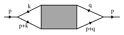
FIG. 1.: The shear viscosity can be expressed as an integral over the 4-point single particle Green function, with two pairs of external legs joined to a point, in the limit of zero external momentum $p$.

Since each composite field $\pi_{ij}$ is made from two single-particle fields $\phi$, the shear viscosity $\eta$ is related to the 4-point Green function of the $\phi$ field, as illustrated in Fig. 1. Substituting $\pi_{ij}$ into Eq. (19) one gets [3, 5]

$$\eta = {{\beta}\over 5}\lim_{p^{0},\mathchoice{{\hbox{\boldmath$\displaystyle p$}}}{{\hbox{\boldmath$\textstyle p$}}}{{\hbox{\boldmath$\scriptstyle p$}}}{{\hbox{\boldmath$\scriptscriptstyle p$}}}\to 0}\int{d^{4}k\over(2\pi)^{4}}\int{d^{4}q\over(2\pi)^{4}}J_{ij}(-k,p{+}k)$$ (20)

$$\times {\rm Im\,}G_{1122}(-k,p{+}k,q,-p{-}q)J^{ij}(q,-p{-}q)\,,$$ (21)

where the function $J_{ij}(p,q)$ joins two $\phi$ propagators to a point (see Fig. 1),

$$J_{ij}(p,q)=p_{i}q_{j}-{\textstyle{1\over 3}}\delta_{ij}\,\mathchoice{{\hbox{\boldmath$\displaystyle p$}}}{{\hbox{\boldmath$\textstyle p$}}}{{\hbox{\boldmath$\scriptstyle p$}}}{{\hbox{\boldmath$\scriptscriptstyle p$}}}\cdot\mathchoice{{\hbox{\boldmath$\displaystyle q$}}}{{\hbox{\boldmath$\textstyle q$}}}{{\hbox{\boldmath$\scriptstyle q$}}}{{\hbox{\boldmath$\scriptscriptstyle q$}}}\,,$$ (22)

and $G_{1122}(-k,p{+}k,q,-p{-}q)$ in Eq.(20) denotes the Fourier-transformed $(1122)$-component of the $\phi$ 4-point Green function. Its 16 CTP components are defined as

$$G_{a_{1}a_{2}a_{3}a_{4}}(x_{1},x_{2},x_{3},x_{4})$$ (23)

$$\quad\equiv(-i)^{3}\left\langle T_{p}\left[\phi_{a_{1}}(x_{1})\phi_{a_{2}}(x_{2})\phi_{a_{3}}(x_{3})\phi_{a_{4}}(x_{4})\right]\right\rangle$$ (24)

$$\quad={\textstyle{1\over 2}}G_{{\alpha}_{1}{\alpha}_{2}{\alpha}_{3}{\alpha}_{4}}(x_{1},x_{2},x_{3},x_{4})Q_{\alpha_{1}a_{1}}Q_{\alpha_{2}a_{2}}Q_{\alpha_{3}a_{3}}Q_{\alpha_{4}a_{4}}\,.$$ (25)

where $G_{{\alpha}_{1}{\alpha}_{2}{\alpha}_{3}{\alpha}_{4}}(x_{1},x_{2},x_{3},x_{4})$ is the corresponding 4-point Green function in the $(r,a)$ basis, defined as [11, 12]

$$G_{{\alpha}_{1}{\alpha}_{2}{\alpha}_{3}{\alpha}_{4}}(x_{1},x_{2},x_{3},x_{4})\equiv(-i)^{3}2^{n_{r}-1}$$ (26)

$$\quad\times\left\langle T_{p}\left[\phi_{{\alpha}_{1}}(x_{1})\phi_{{\alpha}_{2}}(x_{2})\phi_{{\alpha}_{3}}(x_{3})\phi_{{\alpha}_{4}}(x_{4})\right]\right\rangle\,.$$ (27)

Generally, in the $(r,a)$ basis the $n$-point Green function with only $a$ indices vanishes: $G_{aa\dots a}{\,=\,}0$ [12].

B The need for ladder resummation

In the one-loop approximation the 4-point function of Fig. 1 reduces to a product of two 2-point Green functions $\Delta_{12}$ which, in the limit of vanishing external momentum, have opposite momenta. The (12)-component of the 2-point function can be expressed in terms of its spectral function $\rho$ [4]. For noninteracting particles, the poles of the two spectral functions with opposite loop momenta pinch the real axis in the complex energy plane from above and below, resulting in a pinch singularity for the integral over the energy circulating in the loop [16]. This singularity can be cured by using resummed $\phi$ propagators with a two-loop self-energy in the denominator [5, 17, 18]. This resummation generates scalar quasi-particles with a finite thermal (collisional) width and lifetime [18] which shifts the pinching poles away from the real energy axis.

As shown by Jeon [3, 5], however, this regularization of the energy loop integral is not enough to produce a reliable leading-order result for the shear viscosity. We rephrase his arguments, using weakly coupled $\lambda\phi^{4}$ theory as an example. Using the two-loop resummed propagator in the basic one-loop skeleton diagram for $\eta$, the propagator pair sharing the same loop momentum contributes a factor ${\cal O}(1/\lambda^{2})$ to the shear viscosity. (We call this the “nearly pinching poles” contribution.) Clearly such terms involving “nearly pinching poles” are dominant in the weak coupling approximation. For multi-loop ladder diagrams with parallel rungs formed by one-loop diagrams connecting the two “side rail” propagators (see Fig. 2), each pair of side rails shares the same loop momentum as the external momentum $p$ approaches zero; correspondingly, its frequency integral generates a “nearly pinching poles” contribution $\sim 1/\lambda^{2}$ which just compensates the factor $\lambda^{2}$ from the two extra vertices.

All multi-loop ladder diagrams with parallel rungs thus contribute at the same order as the simple one-loop diagram. On the other hand, multi-loop ladders with crossing rungs have different momenta on some of their side rails; since the integrals over the corresponding loop energies are free from “nearly pinching poles” contributions, these diagrams are genuinely suppressed by additional powers of $\lambda^{2}$. Similar arguments rule out leading-order contributions from all other multi-loop diagrams [5]. At leading order we must therefore only resum the infinite ladders with parallel rungs. In the CTP formalism this is achieved by solving a Bethe-Salpeter equation for the 4-point Green function.

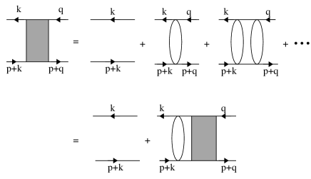
FIG. 2.: In $\lambda\phi^{4}$ theory the summation of an infinite number of planar ladder diagrams contributing to the shear viscosity at leading order results in a Bethe-Salpeter equation for the 4-point Green function.

In the Keldysh basis, the BS integral equation couples the component $G_{1122}$ needed in Eq. (20) to three other components of the 4-point function: $G_{1222}$, $G_{2122}$, and $G_{2222}$. The key technical issue is therefore whether and how the BS equation can be decoupled. In the following we will show that in the weak coupling limit this is indeed possible, and that this is most conveniently achieved in the $(r,a)$ basis: all components of the bare 4-point vertex involving an even number of $a$ indices vanish (see Eq. (113)), and the propagator $\Delta_{aa}{\,=\,}0$ (see Eq. (14)). When decomposing $G_{1122}$ into a linear combination of the sixteen $(r,a)$ 4-point functions an important simplification arises from the generalized FTD [12] (see also [13] and recent work by Guerin[19]) which relates these functions among each other, reducing the number of independent 4-point vertices to seven. We will see that, at leading order in the weak coupling approximation, only one of these seven independent functions contributes to the shear viscosity and its BS equation decouples. Again, the generalized FDT plays an important role in the decoupling procedure.

C Contributions to $\eta$ in the $(r,a)$ basis

Let us now follow the steps of expressing Eq. (20) in $(r,a)$ components. From the KMS condition [20] one derives in momentum space [11, 12]

$$G^{*}_{a_{1}a_{2}a_{3}a_{4}}(k_{1},k_{2},k_{3},k_{4})$$ (28)

$$\qquad=-G_{{\bar{a}}_{1}{\bar{a}}_{2}{\bar{a}}_{3}{\bar{a}}_{4}}(k_{1},k_{2},k_{3},k_{4})\prod_{\{i|a_{i}=2\}}\!\!\!e^{\beta k^{0}_{i}}\,,$$ (29)

where all momenta flow into the vertex such that $k_{1}{+}k_{2}{+}k_{3}{+}k_{4}{\,=\,}0$, the star denotes complex conjugation, and ${\bar{a}}_{i}{\,=\,}2,1$ for $a_{i}{\,=\,}1,2$, respectively. We can thus reexpress $G_{1122}(-k,p{+}k,q,-p{-}q)$ as

$$G_{1122}(-k,p{+}k,q,-p{-}q)$$ (30)

$$\quad=-n(p^{0})\Bigl{(}G_{1122}+G^{*}_{2211}\Bigr{)}(-k,p{+}k,q,-p{-}q).$$ (31)

We combine this with Eq. (23) to decompose ${\rm Im\,}G_{1122}$ in the $(r,a)$ basis:

$${\rm Im\,} G_{1122}(-k,p{+}k,q,-p{-}q)$$ (35)

$$=-n(p^{0}){\rm Im\,}\Bigl{(}G_{1122}+G^{*}_{2211}\Bigr{)}(-k,p{+}k,q,{-}p{-}q)$$

$$={\textstyle{1\over 4}}n(p^{0}){\rm Im\,}\Bigl{(}G_{aaar}{+}G_{aara}{-}G_{araa}{-}G_{raaa}{+}G_{rrra}$$

$$\quad{+}G_{rrar}{-}G_{rarr}{-}G_{arrr}\Bigr{)}(-k,p{+}k,q,-p{-}q)\,.$$

The first four terms on the right hand side involve the fully retarded Green functions defined in [21], $G_{raaa}$, $G_{araa}$, $G_{aara}$, and $G_{aaar}$. They are part of the set of 7 independent 4-point functions chosen in Ref. [12] which additionally includes $G_{arra}$, $G_{arar}$, and $G_{aarr}$. The last four terms in Eq. (35) are not part of this set, but can be expressed through these 7 functions via the generalized FDT [12]:

$$G_{rrra}(k_{1},k_{2},k_{3},k_{4})= \Bigl{[}N_{2}N_{3}G_{raaa}-N_{2}N_{4}N^{(13)}_{(24)}G^{*}_{araa}-N_{3}N_{4}N^{(12)}_{(34)}G^{*}_{aara}-\Bigl{(}N^{(13)}_{(24)}+N_{3}^{2}N^{(12)}_{(34)}\Bigr{)}G^{*}_{aaar}$$ (38)

$$-N_{1}G_{arra}-N_{2}N^{(13)}_{(24)}G^{*}_{arar}-N_{3}N^{(12)}_{(34)}G^{*}_{aarr}\Bigr{]}(k_{1},k_{2},k_{3},k_{4})\,,$$

$$G_{rrar}(k_{1},k_{2},k_{3},k_{4})= \Bigl{[}N_{2}N_{4}G_{raaa}-N_{2}N_{3}N^{(14)}_{(23)}G^{*}_{araa}-\Bigl{(}N^{(12)}_{(34)}+N_{2}^{2}N^{(14)}_{(23)}\Bigr{)}G^{*}_{aara}-N_{3}N_{4}N^{(12)}_{(34)}G^{*}_{aaar}$$ (40)

$$-N_{2}N^{(14)}_{(23)}G^{*}_{arra}-N_{1}G_{arar}-N_{4}N^{(12)}_{(34)}G^{*}_{aarr}\Bigr{]}(k_{1},k_{2},k_{3},k_{4})\,,$$

$$G_{rarr}(k_{1},k_{2},k_{3},k_{4})= \Bigl{[}N_{3}N_{4}G_{raaa}-\Bigl{(}N^{(14)}_{(23)}+N_{4}^{2}N^{(13)}_{(24)}\Bigr{)}G^{*}_{araa}-N_{2}N_{3}N^{(14)}_{(23)}G^{*}_{aara}-N_{2}N_{4}N^{(13)}_{(24)}G^{*}_{aaar}$$ (42)

$$-N_{3}N^{(14)}_{(23)}G^{*}_{arra}-N_{4}N^{(13)}_{(24)}G^{*}_{arar}-N_{1}G_{aarr}\Bigr{]}(k_{1},k_{2},k_{3},k_{4})\,,$$

$$G_{arrr}(k_{1},k_{2},k_{3},k_{4})= \Bigl{[}\Bigl{(}1+N_{2}N_{3}+N_{2}N_{4}+N_{3}N_{4}\Bigr{)}G^{*}_{raaa}-N_{3}N_{4}G_{araa}-N_{2}N_{4}G_{aara}-N_{2}N_{3}G_{aaar}$$ (44)

$$-N_{4}G_{arra}-N_{3}G_{arar}-N_{2}G_{aarr}\Bigr{]}(k_{1},k_{2},k_{3},k_{4})\,.$$

Here $N_{i}{\,=\,}N(k_{i}^{0}){\,=\,}1{+}2n(k_{i}^{0})$ and $N^{(ij)}_{(lm)}{\,=\,}{N_{i}{+}N_{j}\over N_{l}{+}N_{m}}$, with $k^{0}_{1}{+}k^{0}_{2}{+}k^{0}_{3}{+}k^{0}_{4}{\,=\,}0$. Substituting Eqs. (II C) into Eq. (35) we express ${\rm Im\,}G_{1122}(-k,p{+}k,q,-p{-}q)$ as

$${\rm Im\,}G_{1122}(-k,p{+}k,q,-p{-}q)$$ (45)

$$={\rm Im\,}\bigl{[}{\cal A}G_{aarr}+{\cal B}G_{arar}+{\cal C}G_{arra}+{\cal D}G_{raaa}$$ (46)

$$\quad\quad\ +{\cal E}G_{araa}+{\cal F}G_{aara}+{\cal G}G_{aaar}\bigr{]}(-k,p{+}k,q,-p{-}q)\,,$$ (47)

where the coefficients ${\cal A},{\cal B},\cdots,{\cal G}$ involve combinations of thermal distribution functions. In the relevant limit $p^{0}{\,\to\,}0$ they are given, up to terms of order $\beta p^{0}$, by

$${\cal A} \approx -{{\beta p^{0}n(p^{0})}\over 4}(N^{2}_{k}{-}1)\,,$$ (49)

$${\cal B} \approx {\cal C}\approx{\beta p^{0}n(p^{0})\over 8}\Bigl{(}(N^{2}_{k}{-}1)+(N^{2}_{q}{-}1)\Bigr{)},$$ (50)

$${\cal D} \approx {\cal F}+{\cal G}\,,$$ (51)

$${\cal E} \approx 0\,,$$ (52)

$${\cal F} \approx {\beta p^{0}n(p^{0})\over 8}\Bigl{(}N_{k}(N^{2}_{q}{-}1)+N_{q}(N^{2}_{k}{-}1)\Bigr{)},$$ (53)

$${\cal G} \approx {\beta p^{0}n(p^{0})\over 8}\Bigl{(}N_{k}(N^{2}_{q}{-}1)-N_{q}(N^{2}_{k}{-}1)\Bigr{)}.$$ (54)

Here $N_{k}{\,=\,}N(k^{0}){\,=\,}1{+}2n(k^{0})$ and similarly for $N_{q}$. In the zero external momentum limit the explicitly shown terms are finite since $\lim_{p^{0}\to 0}\beta p^{0}\,n(p^{0})=1$, whereas the dropped terms of order $\beta p^{0}$ and higher vanish. Since ${\cal E}{\,=\,0}$ in this limit, $G_{araa}$ does not contribute to the shear viscosity.

The $n$-point functions involving only elementary fields $\phi$ are symmetric under particle exchange:

$$G_{\dots\alpha_{i}\dots\alpha_{j}\dots}(\dots,k_{i},\dots,k_{j},\dots)$$ (55)

$$\quad=G_{\dots\alpha_{j}\dots\alpha_{i}\dots}(\dots,k_{j},\dots,k_{i},\dots)\,.$$ (56)

Moreover, the factor $J_{ij}(-k,k)J^{ij}(q,-q)$ in Eq. (20) is invariant under each of the following changes of integration variables: $k{\,\leftrightarrow\,}q$, $k{\,\leftrightarrow\,}{-}k$ and $q{\,\leftrightarrow\,}{-}q$. Using Eq. (55), both $G_{raaa}({-}k,k,q,{-}q)$ under the variable change $k{\,\leftrightarrow\,}q$ and $G_{aara}({-}k,k,q,{-}q)$ under the variable change $q{\,\rightarrow\,}{-}q$ become equal to $G_{aaar}({-}k,k,q,{-}q)$. Performing the same variable changes on the corresponding prefactors ${\cal D}$ and ${\cal F}$ we can substitute in Eq. (20)

$$[{\cal D}G_{raaa} + {\cal F}G_{aara}+{\cal G}G_{aaar}](-k,k,q,-q)$$ (57)

$$\to {\textstyle{1\over 4}}N_{k}(N_{q}^{2}{-}1)\,G_{aaar}(-k,k,q,-q).$$ (58)

Using Eq. (55) together with $N({-}k^{0}){\,=\,}{-}N(k^{0})$ this is seen to be an odd function of $k$ which integrates to zero in Eq. (20). Consequently, none of the four fully retarded 4-point functions contributes to the shear viscosity.

Similarly, under the variable change $q{\,\rightarrow\,}{-}q$ we have $G_{arar}({-}k,k,q,{-}q){\,\to\,}G_{arra}({-}k,k,q,{-}q)$ such that

$$[{\cal B}G_{arar}+{\cal C}G_{arra}](-k,k,q,-q)$$ (59)

$$\qquad\to{\textstyle{1\over 4}}\Bigl{(}(N_{k}^{2}{-}1)+(N_{q}^{2}{-}1)\Bigr{)}G_{arra}(-k,k,q,-q)$$ (60)

$$\qquad\to{\textstyle{1\over 2}}(N_{k}^{2}{-}1)G_{arra}(-k,k,q,-q)\,,$$ (61)

where the second substitution involves the variable change $k{\,\leftrightarrow\,}q$. We will see below that in the weak coupling limit this term does not contribute to $\eta$ at leading order either, leaving only the contribution from $G_{aarr}$.

D Bethe-Salpeter equation for $G_{\alpha_{1}\alpha_{2}\alpha_{3}\alpha_{4}}$

Referring to Fig. 2 above and Fig. 5 further below, the BS equation for the 4-point Green function $G_{\alpha_{1}\alpha_{2}\alpha_{3}\alpha_{4}}$ can be expressed in the $(r,a)$ basis as

$$i^{3}G_{\alpha_{1}\alpha_{2}\alpha_{3}\alpha_{4}}(-k,k,q,-q)=$$ (62)

$$\left[i\Delta_{\alpha_{1}\alpha_{3}}(-k)\right]\left[i\Delta_{\alpha_{2}\alpha_{4}}(k)\right](2\pi)^{4}\delta^{4}(k{-}q)+$$ (63)

$$\left[i\Delta_{\alpha_{1}\beta_{1}}(-k)\right]\left[i\Delta_{\alpha_{2}\gamma_{1}}(k)\right]\int{d^{4}l\over(2\pi)^{4}}K_{\beta_{1}\gamma_{1}\beta_{4}\gamma_{4}}(-k,k,l,-l)$$ (64)

$$\ \times\left[i^{3}G_{\beta_{4}\gamma_{4}\alpha_{3}\alpha_{4}}(-l,l,q,-q)\right]\,.$$ (65)

As always repeated indices are summed over, and $K_{\beta_{1}\gamma_{1}\beta_{4}\gamma_{4}}$ is the kernel (an amputed 1PI 4-point vertex function) of the integral equation. For the component $G_{arra}$ we have

$$G_{arra}(-k,k,q,-q)$$ (66)

$$\quad=-i\Delta_{ra}(k)\Delta_{ra}(k)(2\pi)^{4}\delta^{4}(k{-}q)$$ (67)

$$\quad-\Delta_{ra}(k)\Delta_{rr}(k)\int{d^{4}l\over(2\pi)^{4}}K_{rr\beta_{4}\gamma_{4}}(-k,k,l,-l)$$ (68)

$$\qquad\times G_{\beta_{4}\gamma_{4}ra}(-l,l,q,-q)$$ (69)

$$\quad-\Delta_{ra}(k)\Delta_{ra}(k)\int{d^{4}l\over(2\pi)^{4}}K_{ra\beta_{4}\gamma_{4}}(-k,k,l,-l)$$ (70)

$$\qquad\times G_{\beta_{4}\gamma_{4}ra}(-l,l,q,-q)\,.$$ (71)

Here we used $\Delta_{\alpha_{1}\alpha_{2}}({-}k){\,=\,}\Delta_{\alpha_{2}\alpha_{1}}(k)$ and $\Delta_{aa}(k){\,=\,}0$. In the second term we can reexpress $\Delta_{rr}$ in terms of $\Delta_{ra}$ and $\Delta_{ar}$ using the FDT (15). Since $\Delta_{ra}(k)$ and $\Delta_{ar}(k)$ are retarded and advanced Green functions, respectively, the poles of $\Delta_{ra}(k)\Delta_{ra}(k)$ and $\Delta_{ar}(k)\Delta_{ar}(k)$ in the complex $k^{0}$ plane lie on the same side of the real $k^{0}$ axis. Hence, in the limit $\lambda{\,\to\,}0$, they do not generate a pinch singularity in the integrand of Eq. (20). The term $\sim\Delta_{ra}(k)\Delta_{ar}(k){\,=\,}|\Delta_{ra}(k)|^{2}$, on the other hand, does generate a pinch singularity as $\lambda{\,\to\,}0$; in the weak coupling limit, this term will thus dominate in Eq. (20) over the two other ones. With this “nearly pinching poles” approximation we can rewrite Eq. (66) as

$$G_{arra}(-k,k,q,-q)=N(k^{0})|\Delta_{ra}(k)|^{2}$$ (72)

$$\quad\times\int{d^{4}l\over(2\pi)^{4}}K_{rr\beta_{4}\gamma_{4}}(-k,k,l,-l)\,G_{\beta_{4}\gamma_{4}ra}(-l,l,q,-q)\,.$$ (73)

Using $N({-}k^{0}){\,=\,}{-}N(k^{0})$ and the analogue of the symmetry relations (55) for the amputated 1PI vertex [12], we see that ${1\over 2}(N_{k}^{2}{-}1)G_{arra}(-k,k,q,-q)$ is an odd function of $k$ and thus gives a vanishing leading order contribution to the shear viscosity in Eq. (20). This leaves only $G_{aarr}$:

$$\eta = -{\beta\over 5}\int{d^{4}k\over(2\pi)^{4}}n(k^{0})\bigl{(}1{+}n(k^{0})\bigr{)}I_{\pi,lm}(k)$$ (75)

$$\times\int{d^{4}q\over(2\pi)^{4}}{\rm Im\,}G_{aarr}(-k,k,q,-q)I_{\pi}^{lm}(q)\,.$$

Here $I_{\pi,lm}(k)\equiv-J_{lm}(-k,k)$ is the notation used in [5].

E Decoupling the BS equation for $G_{aarr}$

We now show that the BS equation for $G_{aarr}$ decouples from the other components of $G_{\alpha_{1}\alpha_{2}\alpha_{3}\alpha_{4}}$ in the “nearly pinching poles” approximation. From Eq. (62) we obtain

$$G_{aarr}(-k,k,q,-q)$$ (76)

$$\quad=-\Delta_{ra}(k)\Delta_{ar}(k)\Bigl{[}i(2\pi)^{4}\delta^{4}(k{-}q)$$ (77)

$$\quad+\int{d^{4}l\over(2\pi)^{4}}K_{rr\beta_{4}\gamma_{4}}(-k,k,l,-l)G_{\beta_{4}\gamma_{4}rr}(-l,l,q,-q)\Bigr{]}$$ (78)

$$\quad=-\Delta_{ra}(k)\Delta_{ar}(k)\Bigl{\{}i(2\pi)^{4}\delta^{4}(k{-}q)$$ (79)

$$\quad+\int{d^{4}l\over(2\pi)^{4}}\Bigl{[}K_{rrra}(-k,k,l,-l)G_{rarr}(-l,l,q,-q)$$ (80)

$$\qquad\qquad+K_{rrar}(-k,k,l,-l)G_{arrr}(-l,l,q,-q)$$ (81)

$$\qquad\qquad+K_{rraa}(-k,k,l,-l)G_{aarr}(-l,l,q,-q)\Bigr{]}\Bigr{\}}\,.$$ (82)

For the second equality we used $K_{rrrr}{\,=\,}0$ which is the analogue for the amputated 1PI 4-point vertex of the previously mentioned relation $G_{aaaa}{\,=\,}0$ [12]. At this point $G_{aarr}$ still couples to $G_{rarr}$ and $G_{arrr}$. For later convenience we introduce a function $M$ which is obtained by truncating two of the external legs of the 4-point Green function $G$:

$$G_{\alpha_{1}\alpha_{2}\alpha_{3}\alpha_{4}}(-l,l,q,-q)=$$ (83)

$$\left[i\Delta_{\alpha_{1}\beta_{1}}(-l)\right]\left[i\Delta_{\alpha_{2}\beta_{2}}(l)\right]M_{\beta_{1}\beta_{2}\alpha_{3}\alpha_{4}}(-l,l,q,-q)\,.$$ (84)

It follows that

$$G_{aarr} (-l,l,q,-q)$$ (86)

$$=-\Delta_{ra}(l)\Delta_{ar}(l)M_{rrrr}(-l,l,q,-q)\,.$$

As above we now use the “nearly pinching poles” approximation, ignoring terms involving $\Delta_{ra}(l)\Delta_{ra}(l)$ and $\Delta_{ar}(l)\Delta_{ar}(l)$ relative to terms involving $\Delta_{ra}(l)\Delta_{ar}(l)$. Using Eqs. (14) and (15), we can then write

$$G_{rarr} (-l,l,q,-q)$$ (90)

$$=-N(l^{0})\Delta_{ra}(l)\Delta_{ar}(l)M_{rrrr}(-l,l,q,-q)$$

$$=N(l^{0})G_{aarr}(-l,l,q,-q)\,,$$

$$G_{arrr} (-l,l,q,-q)$$ (93)

$$=N(l^{0})\Delta_{ra}(l)\Delta_{ar}(l)M_{rrrr}(-l,l,q,-q)$$

$$=-N(l^{0})G_{aarr}(-l,l,q,-q)\,.$$

These leading order relations decouple the BS equation (76) for $G_{aarr}$; we find

$$G_{aarr}(-k,k,q,-q)$$ (94)

$$\quad=-\Delta_{ra}(k)\Delta_{ar}(k)\Bigl{[}i(2\pi)^{4}\delta^{4}(k{-}q)$$ (95)

$$\quad+\int{d^{4}l\over(2\pi)^{4}}\,{\cal K}(-k,k,l,-l)\,G_{aarr}(-l,l,q,-q)\Bigr{]}$$ (96)

with the kernel

$${\cal K} (-k,k,l-l)=$$ (98)

$$\Bigl{(}N(l^{0})\left(K_{rrra}{-}K_{rrar}\right)+K_{rrra}\Bigr{)}(-k,k,l,-l)\,.$$

F An integral equation for the viscosity

For further simplification we introduce the 2-point spectral density

$$\rho(k)=i[\Delta_{ra}(k)-\Delta_{ar}(k)]\,.$$ (99)

Writing the full retarded propagator $\Delta_{ra}(k)$ as

$$\Delta_{ra}(k)={1\over{k^{2}-{\rm Re\,}\Sigma(k)+i\,{\rm Im\,}\Sigma(k)}}$$ (100)

and using $\Delta_{ar}(k){\,=\,}\Delta^{*}_{ra}(k)$ we deduce

$$\rho(k)={{2\,{\rm Im\,}\Sigma(k)}\over{\bigl{(}k^{2}-{\rm Re\,}\Sigma(k)\bigr{)}^{2}+\bigl{(}{\rm Im\,}\Sigma(k)\bigr{)}^{2}}}\,,$$ (101)

$$\Delta_{ra}(k)\Delta_{ar}(k)=|\Delta_{ra}(k)|^{2}={\rho(k)\over{2{\rm Im\,}\Sigma(k)}}\,.$$ (102)

Substituting Eq. (102) into Eq. (86) we get

$${\rm Im\,}G_{aarr} (-k,k,q,-q)=$$ (104)

$$-{\rho(k)\over{2{\rm Im\,}\Sigma(k)}}{\rm Im\,}M_{rrrr}(-k,k,q,-q)\,,$$

and the decoupled BS equation (94) can be written as

$${\rm Im\,}M_{rrrr}(-k,k,q,-q)=(2\pi)^{4}\delta^{4}(k{-}q)$$ (105)

$$+\int{d^{4}l\over(2\pi)^{4}}{\rho(l)\over{2{\rm Im\,}\Sigma(l)}}{\cal K}(-k,k,l,-l){\rm Im\,}M_{rrrr}(-l,l,q,-q).$$ (106)

Defining further

$$D_{\pi}^{lm}(k)=\int{d^{4}q\over(2\pi)^{4}}\,I_{\pi}^{lm}(q)\,{\rm Im\,}M_{rrrr}(-k,k,q,-q)$$ (107)

and using it in Eqs. (75) and (105) we finally arrive at

$$\eta={\beta\over 10}{\int}{d^{4}k\over(2\pi)^{4}}\,n(k^{0})\bigl{(}1{+}n(k^{0})\bigr{)}{\rho(k)\,I_{\pi}(k)\cdot D_{\pi}(k)\over{\rm Im\,}\Sigma(k)}.$$ (108)

Here $I_{\pi}\cdot D_{\pi}\equiv I_{\pi,lm}D_{\pi}^{lm}$, and $D_{\pi}(k)$ satisfies the integral equation (suppressing the tensor indices on $I_{\pi},D_{\pi}$)

$$D_{\pi}(k)=I_{\pi}(k)-{\int}{d^{4}l\over(2\pi)^{4}}{\cal K}(-k,k,l,-l)\,{\rho(l)\,D_{\pi}(l)\over{2\,{\rm Im\,}\Sigma(l)}}.$$ (109)

These last two expressions were previously obtained in [5, 6]. The present derivation, however, does not use a specific form of the interaction Lagrangian; within the “nearly pinching poles” approximation, Eqs. (108) and (109) form a general result for all scalar field theories, with different forms of the interaction Lagrangian resulting in different kernels ${\cal K}(-k,k,l,-l)$. We expect a similar integral equation to hold for the leading order viscosity in pure (quarkless) QCD, with modified expressions for $I_{\pi}$ and ${\cal K}$. In the following Section, we evaluate ${\cal K}$ in the CTP formalism for the $\lambda\phi^{4}$ and $g\phi^{3}{+}\lambda\phi^{4}$ theories and show that the results agree with those obtained by Jeon [5] in the imaginary time formalism.

III The shear viscosity kernel in scalar field theories

A Massless $\lambda\phi^{4}$ theory

The Lagrangian for massless $\phi^{4}$ theory reads

$${\cal L}_{0}={1\over 2}(\partial_{\mu}\phi)^{2}-{\lambda\over 4!}\phi^{4},$$ (110)

and we consider it in the weak coupling limit $\lambda\ll 1$. For this theory the kernel of the integral equation (see Fig. 2) can be expressed as

$$K_{\beta_{1}\gamma_{1}\beta_{4}\gamma_{4}} (-k,k,l,-l)={1\over 2}{\int}{d^{4}s\over(2\pi)^{4}}\lambda_{\gamma_{1}\gamma_{2}\gamma_{3}\gamma_{4}}\lambda_{\beta_{1}\beta_{2}\beta_{3}\beta_{4}}$$ (112)

$$\times\Delta_{\gamma_{2}\beta_{2}}(s)\Delta_{\gamma_{3}\beta_{3}}(s+l-k)\,,$$

where the prefactor ${1\over 2}$ is the symmetry factor associated with the bubble connecting the two lines, and the bare 4-point vertex in the $(r,a)$ basis is given by [12]

$$\lambda_{\alpha_{1}\alpha_{2}\alpha_{3}\alpha_{4}}={\lambda\over 4}\Bigl{(}1-(-1)^{n_{a}}\Bigr{)}\,,$$ (113)

$n_{a}$ being the number of $a$ indices among $(\alpha_{1},\alpha_{2},\alpha_{3},\alpha_{4})$. The last equation implies that all bare vertices must involve an odd number of $a$ indices (in particular $\lambda_{rrrr}{\,=\,}0$).

Using Eq. (113) and $\Delta_{aa}(k)=0$, Eq. (112) gives

$$K {}_{rrra}(-k,k,l,-l)={\lambda^{2}\over 8}{\int}{d^{4}s\over(2\pi)^{4}}$$ (116)

$$\quad\times\Bigl{[}\Delta_{rr}(s)\Delta_{ar}(s{+}l{-}k)+\Delta_{ra}(s)\Delta_{rr}(s{+}l{-}k)\Bigr{]}\,,$$

$$K {}_{rrar}(-k,k,l,-l)={\lambda^{2}\over 8}\int{d^{4}s\over(2\pi)^{4}}$$ (118)

$$\quad\times\Bigl{[}\Delta_{ar}(s)\Delta_{rr}(s{+}l{-}k)+\Delta_{rr}(s)\Delta_{ra}(s{+}l{-}k)\Bigr{]}\,,$$

$$K {}_{rraa}(-k,k,l,-l)={\lambda^{2}\over 8}\int{d^{4}s\over(2\pi)^{4}}\Bigl{[}\Delta_{rr}(s)\Delta_{rr}(s{+}l{-}k)$$ (120)

$$\quad+\Delta_{ra}(s)\Delta_{ar}(s{+}l{-}k)+\Delta_{ar}(s)\Delta_{ra}(s{+}l{-}k)\Bigr{]}\,.$$

Noticing that the $s^{0}$-integrals over terms of the type $\Delta_{ra}(s)\Delta_{ra}(s{+}l{-}k)$ and $\Delta_{ar}(s)\Delta_{ar}(s{+}l{-}k)$ vanish because the poles of these two terms are both on the same side of the real axis in the complex $s^{0}$ plane, we can make the following replacement:

$$\int{d^{4}s\over(2\pi)^{4}}\Bigl{[}\Delta_{ra}(s)\Delta_{ar}(s{+}l{-}k)+\Delta_{ar}(s)\Delta_{ra}(s{+}l{-}k)\Bigr{]}$$ (121)

$$={\int}{d^{4}s\over(2\pi)^{4}}\bigl{[}\Delta_{ra}(s){-}\Delta_{ar}(s)\bigr{]}\bigl{[}\Delta_{ar}(s{+}l{-}k){-}\Delta_{ra}(s{+}l{-}k)\bigr{]}$$ (122)

$$=\int{d^{4}s\over(2\pi)^{4}}\,\rho(s)\,\rho(s{+}l{-}k)\,.$$ (123)

Inserting Eqs. (III A) into Eq. (98) and using Eqs. (15), (99) and (121), we express the kernel of the BS equation as

$${\cal K}^{(\phi^{4})}(-k,k,l,-l)={\lambda^{2}\over 2}\int d[s_{1},s_{2}]\,,$$ (124)

introducing for later convenience the shorthand notation

$$\int d[s_{1},s_{2}]\equiv-{{1+n(l^{0})}\over{1+n(k^{0})}}\int{d^{4}s_{1}\over(2\pi)^{4}}{d^{4}s_{2}\over(2\pi)^{4}}\bigl{(}1{+}n(s_{1}^{0})\bigr{)}\rho(s_{1})$$ (125)

$$\qquad\times\bigl{(}1{+}n({-}s_{2}^{0})\bigr{)}\rho(-s_{2})\,(2\pi)^{4}\delta^{4}(s_{1}{-}s_{2}{+}l{-}k)\,.$$ (126)

Substituting this into Eq.(109) we obtain

$$D_{\pi}(k)=I_{\pi}(k)+{\lambda^{2}\over 4}{\int}{d^{4}l\over(2\pi)^{4}}{1{+}n(l^{0})\over 1{+}n(k^{0})}\,{\rho(l)\,D_{\pi}(l)\over{\rm Im\,}\Sigma(l)}$$ (127)

$$\quad\times{\int}{d^{4}s\over(2\pi)^{4}}n(s^{0})\rho(s)\bigl{(}1{+}n(s^{0}{+}k^{0}{-}l^{0})\bigr{)}\rho(s{+}k{-}l)\,.$$ (128)

The shear viscosity is obtained by inserting the solution of this integral equation into Eq. (108). This result coincides with that obtained by Jeon [5] in the ITF.

B Massive $g\phi^{3}+\lambda\phi^{4}$ theory

1 The $\phi$ self energy

We now investigate the contributions arising from an additional cubic interaction. For massless scalar fields, it renders the zero temperature theory perturbatively unstable, causing a nonzero vacuum expectation value for $\phi$. To avoid this we introduce a nonzero mass $m$ for the scalar field and study [5]

$${\cal L}_{0}={1\over 2}(\partial_{\mu}\phi)^{2}-{m^{2}\over 2}\phi^{2}-{g\over 3!}\phi^{3}-{\lambda\over 4!}\phi^{4}+{\cal L}_{c}$$ (129)

in the weak-coupling limit $(g/m)^{2}{\,\lesssim\,}\lambda{\,\ll\,}1$. $m$, $g$, and $\lambda$ denote the physical mass and coupling constants at zero temperature, and ${\cal L}_{c}$ denotes the counter terms required for renormalization. The one- and two-loop diagrams for the self-energy in this theory are shown in Figs. 3 and 4.

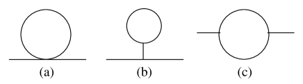
FIG. 3.: One-loop self-energy diagrams in $g\phi^{3}{+}\lambda\phi^{4}$ theory.

Diagrams 3(a) and 3(b) are independent of the external momentum which does not enter the loop; they generate a purely real contribution ${\cal O}(\lambda T^{2}{-}g^{2}T^{2}/m^{2})$ to the scalar self energy. For $T{\,\ll\,}m/\sqrt{\lambda}$ this is much smaller than $m^{2}$, and the viscosity can thus be calculated using the zero-temperature mass $m$ in all propagators [5]. For $T{\,\gtrsim\,}m/\sqrt{\lambda}$, the thermal self energy becomes comparable to $m^{2}$ and must be resummed, yielding quasi-particles with a thermal mass of order $m_{\rm th}^{2}{\,\sim\,}\lambda T^{2}$ [5, 17, 18]. For $T{\,\gg\,}m/\sqrt{\lambda}$ the self-energy from diagram 3(b) is then ${\sim\,}{-}g^{2}T^{2}/m_{\rm th}^{2}$; due to the weak-coupling condition $g^{2}{\,\lesssim\,}\lambda m^{2}$ this is smaller than diagram 3(a) by a factor $m^{2}/m_{\rm th}^{2}{\,\sim\,}m^{2}/(\lambda T^{2}){\,\ll\,}1$. At such high temperatures, the effects from the 4-point interaction thus dominate those from the 3-point interaction, and the theory becomes effectively a massless $\lambda\phi^{4}$ theory as discussed in the previous subsection. We thus concentrate on the interesting temperature range $T{\,\sim\,}m/\sqrt{\lambda}$ where on the one hand mass resummation is required but on the other hand $\phi^{3}$ interaction effects are not yet negligible.

The lowest order contribution to the imaginary part of the scalar self energy arises from diagram 3(c). It vanishes on-shell (an on-shell particle cannot decay into two on-shell particles with the same thermal mass) but is non-zero and ${\cal O}(g^{2})$ for off-shell momenta. Its real part is smaller than that of Figs. 3(a,b) and does not contribute to the leading-order thermal mass [5]. The imaginary contribution vanishes for the side rails of the multi-ladder diagrams in the “nearly pinching poles” approximation which forces the side rail momenta approximately on-shell, but it plays an important role for single-line rungs in the BS equation generated by the exchange of a single scalar field (see Fig. 5(b) below).

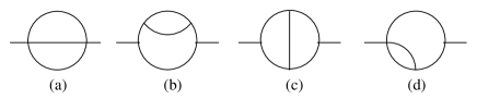
FIG. 4.: Two-loop self-energy diagrams in $g\phi^{3}{+}\lambda\phi^{4}$ theory.

The leading order contribution to the on-shell imaginary part of the self-energy arises from the two-loop diagrams in Fig. 4. As shown in detail in [5], it is ${\cal O}(\lambda^{2}T^{2})$ (this includes the contributions from diagrams 4(b-c) in the weak-coupling limit $(g/m)^{2}{\,\sim\,}\lambda{\,\ll\,}1$). It results in an ${\cal O}(1/(\lambda^{2}T))$ thermal lifetime for the quasi-particles [5, 17, 18]. Just as in the simpler $\phi^{4}$ theory, the frequency integral over pairs of propagators from the side rails of the multi-ladder diagram sharing the same loop momentum is proportional to the quasi-particle lifetime. The corresponding factor $1/\lambda^{2}{\,\sim\,}m^{2}/(g^{2}\lambda){\,\sim\,}(m/g)^{4}$ compensates for the extra coupling constants from the vertices associated with the rung. Thus again an infinite number of ladder diagrams contributes to the leading order shear viscosity; they will be resummed through the BS equation.

2 The BS kernel for $g\phi^{3}+\lambda\phi^{4}$ theory

The various contributions to the kernel of the BS equation for the leading order shear viscosity in $g\phi^{3}+\lambda\phi^{4}$ theory are illustrated in Fig. 5. Whereas for the side rails of the ladder full (i.e. at least two-loop resummed) propagators must be used, in order to regulate the pinch singularity in the integral over the side rail momentum, it is sufficient at leading order to use bare propagators in the contributions to the rungs of the ladder shown in Fig. 5 [5]. We will nonetheless formally evaluate them with full propagators, in keeping with the spirit of our skeleton diagram expansion, even though we will not make use of the implied higher order corrections which, for a consistent treatment, would also require the resummation of non-ladder diagrams and ladders with crossed rungs.

Diagram 5(a) corresponds to the pure $\phi^{4}$ theory discussed in the previous subsection. For pure $\phi^{3}$ theory, one might think that the simplest kernel for the ladder diagrams should arise from the single straight line rung (one-particle exchange) (not shown in Fig. 5). Using naive power counting, this straight-line kernel would contribute only two powers of $g$ from the explicit vertices which cannot even compensate for the “nearly pinching poles” contribution ${\sim\,}1/\lambda^{2}{\,\sim\,}(m/g)^{4}$ from the frequency integral over the pair of side rail propagators with the same loop momentum. If this were correct, in the weak-coupling limit each further single-line rung on the ladder would make the shear viscosity more singular. Fortunately, this fear is unnecessary: due to the nearly pinching poles from the pairs of rail propagators, the loop integrals are dominated by almost on-shell rail momenta. For non-zero values of the overall loop momentum $k$ in Eq. (20) this forces all rung momenta off-shell. In the $(r,a)$ basis, only vertices with an odd number of $a$ indices are non-zero; together with $\Delta_{aa}(k){\,=\,}0$ this implies that the kernel from the straight line rung is proportional to the spectral density of the $\phi$ propagator (see Eq. (138) below). For off-shell momenta, this spectral density vanishes at tree level, so the single straight line rung with a bare exchanged propagator does not contribute.

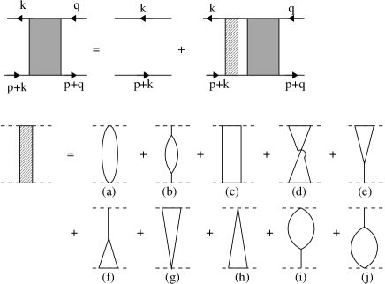
FIG. 5.: Graphic representation of the Bethe-Salpeter equation for the 4-point Green function in $g\phi^{3}{+}\lambda\phi^{4}$ theory. Compared to the pure $\lambda\phi^{4}$ theory shown in Fig. 2, the kernel giving the leading order contribution to the shear viscosity (shown in the second and third line) is more elaborate. With $(g/m)^{2}{\,\sim\,}\lambda$, all contributions to the kernel are of order $\lambda^{2}$.

A non-zero contribution to the kernel from single particle exchange thus requires at least 1-loop accuracy for the propagator of the single-line rung; this is shown in Fig. 5(b). As discussed in the preceding subsection, the loop in diagram 3(c) contributes an imaginary part of order $g^{2}$ to the single-particle self-energy and spectral density which is non-zero for off-shell momenta. Together with the two factors $g$ from the vertices on the side rail this renders the kernel from Fig. 5(b) ${\cal O}\bigl{(}(g/m)^{4}\bigr{)}$ and thus of the same order as all other diagrams in Fig. 5 (which involve the exchange of more than one particle). Note that, whereas the exchange of a single bare propagator contributes zero to the BS kernel, its once iterated version, shown in Fig. 5(c), is non-zero and again of order ${\cal O}\bigl{(}(g/m)^{4}\bigr{)}$ [5].

3 The individual contributions to the kernel

The kernel from diagram 5(a) is given by Eq. (124):

$${\cal K}^{(a)}(-k,k,l,-l)={\lambda^{2}\over 2}\int d[s_{1},s_{2}].$$ (130)

The other contributions are calculated in a similar way. We show the calculational process in some detail for diagrams 5(b) and 5(c), but only mention a few key steps and list the final results for diagrams 5(d-j).

In the $(r,a)$ basis the bare 3-point vertex is given by

$$g_{\alpha_{1}\alpha_{2}\alpha_{3}}={g\over{2^{3/2}}}\Bigl{(}1-(-1)^{n_{a}}\Bigr{)}\,,$$ (131)

where $n_{a}$ is the number of $a$ indices among $(\alpha_{1},\alpha_{2},\alpha_{3})$. Explicitly this reads $g_{rrr}{\,=\,}g_{raa}{\,=\,}g_{ara}{\,=\,}g_{aar}{\,=\,}0$, $g_{aaa}=g_{rra}=g_{rar}=g_{arr}=g/\sqrt{2}$.

For the single-particle exchange Fig. 5(b) the general expression for the kernel can be written as

$$K^{(b)}_{\alpha_{1}\beta_{1}\alpha_{3}\beta_{3}}(-k,k,l,-l)$$ (132)

$$\quad=-ig_{\alpha_{1}\alpha_{2}\alpha_{3}}g_{\beta_{1}\beta_{2}\beta_{3}}\Delta_{\beta_{2}\alpha_{2}}(k{-}l)$$ (133)

where $\Delta$ is the full single-particle propagator. With Eq. (131) we get

$$K^{(b)}_{rrra}(-k,k,l,-l) = -i{g^{2}\over 2}\Delta_{ra}(k{-}l)\,,$$ (135)

$$K^{(b)}_{rrar}(-k,k,l,-l) = -i{g^{2}\over 2}\Delta_{ar}(k{-}l)\,,$$ (136)

$$K^{(b)}_{rraa}(-k,k,l,-l) = -i{g^{2}\over 2}\Delta_{rr}(k{-}l)\,.$$ (137)

Inserting these into Eq. (98) and using Eqs. (15), (99) and (102) we obtain

$${\cal K}^{(b)}(-k,k,l,-l)=-{g^{2}\over 2}[N(l^{0})+N(k^{0}{-}l^{0})]\,\rho(k{-}l)$$ (138)

$$\ \ =-g^{2}[N(l^{0}){+}N(k^{0}{-}l^{0})]\bigl{|}\Delta_{ra}(k{-}l)\bigr{|}^{2}\,{\rm Im}\,\Sigma(k{-}l)\,.$$ (139)

As promised, the kernel for diagram 5(b) is proportional to the spectral density (or the imaginary part of the self-energy). For off-shell $k{-}l$ the lowest order contribution to Im $\Sigma$ is given by diagram 3(c):

$${\rm Im}\,\Sigma(k{-}l)={1\over 2i}\Bigl{(}\Sigma_{ra}(k{-}l)-\Sigma_{ar}(k{-}l)\Bigr{)}$$ (140)

$$\quad={g^{2}\over 8}{\int}{d^{4}s\over(2\pi)^{4}}\Bigl{\{}\Delta_{rr}(s)\bigl{[}\Delta_{ar}(s{+}k{-}l){-}\Delta_{ra}(s{+}k{-}l)\bigr{]}$$ (141)

$$\qquad\qquad+\bigr{[}\Delta_{ra}(s){-}\Delta_{ar}(s)\bigr{]}\Delta_{rr}(s{+}k{-}l)\Bigr{\}}\,.$$ (142)

Using Eqs. (15), (99) and the identity

$$n(z_{1}{+}z_{2}{+}\cdots{+}z_{n})=$$ (143)

$${{n(z_{1})n(z_{2})\cdots n(z_{n})}\over{[1{+}n(z_{1})][1{+}n(z_{2})]\cdots[1{+}n(z_{n})]{-}n(z_{1})n(z_{2})\cdots n(z_{n})}}\,,$$ (144)

we can insert Eq. (140) back into Eq. (138). With a little algebra we find that the result can be written in the form

$${\cal K}^{(b)}(-k,k,l,-l)={g^{4}\over 2}\int d[s_{1},s_{2}]\,\bigl{|}\Delta_{ra}(s_{1}{-}s_{2})\bigr{|}^{2}\,,$$ (145)

where we used the $\delta$-function in Eq. (125) to replace $k{-}l{\,=\,}s_{1}{-}s_{2}$.

For diagram 5(c) the kernel can be expressed as

$$K^{(c)}_{\alpha_{1}\beta_{1}\gamma_{3}\delta_{3}}(-k,k,l,-l)=g_{\alpha_{1}\alpha_{2}\alpha_{3}}g_{\beta_{1}\beta_{2}\beta_{3}}g_{\gamma_{1}\gamma_{2}\gamma_{3}}g_{\delta_{1}\delta_{2}\delta_{3}}$$ (146)

$$\quad\times\int{d^{4}s\over(2\pi)^{4}}\Delta_{\beta_{2}\alpha_{2}}(s)\Delta_{\gamma_{2}\delta_{2}}(s{+}l{-}k)$$ (147)

$$\qquad\qquad\quad\!\times\,\Delta_{\beta_{3}\delta_{1}}(k{-}s)\Delta_{\gamma_{1}\alpha_{3}}(k{-}s)\,.$$ (148)

With Eqs. (131), (14), and (15) and dropping the terms involving $\Delta_{ra}(k{-}s)\Delta_{ra}(k{-}s)$ and $\Delta_{ar}(k{-}s)\Delta_{ar}(k{-}s)$, we obtain

$$K^{(c)}_{rrra}(-k,k,l,-l)$$ (150)

$$\quad={g^{4}\over 4}{\int}{d^{4}s\over(2\pi)^{4}}\bigl{|}\Delta_{ra}(k{-}s)\bigr{|}^{2}\Delta_{ar}(s{+}l{-}k)$$ (151)

$$\qquad\ \times\Bigl{[}\Delta_{rr}(s)+N(k^{0}{-}s^{0})\Bigl{(}\Delta_{ra}(s){-}\Delta_{ar}(s)\Bigr{)}\Bigr{]}\,,$$ (152)

$$K^{(c)}_{rrar}(-k,k,l,-l)$$ (153)

$$\quad={g^{4}\over 4}{\int}{d^{4}s\over(2\pi)^{4}}\bigl{|}\Delta_{ra}(k{-}s)\bigr{|}^{2}\Delta_{ra}(s{+}l{-}k)$$ (154)

$$\qquad\ \times\Bigl{[}\Delta_{rr}(s)+N(k^{0}{-}s^{0})\Bigl{(}\Delta_{ra}(s){-}\Delta_{ar}(s)\Bigr{)}\Bigr{]}\,,$$ (155)

$$K^{(c)}_{rraa}(-k,k,l,-l)$$ (156)

$$\quad={g^{4}\over 4}{\int}{d^{4}s\over(2\pi)^{4}}\bigl{|}\Delta_{ra}(k{-}s)\bigr{|}^{2}\Delta_{rr}(s{+}l{-}k)$$ (157)

$$\qquad\ \times\Bigl{[}\Delta_{rr}(s)+N(k^{0}{-}s^{0})\Bigl{(}\Delta_{ra}(s){-}\Delta_{ar}(s)\Bigr{)}\Bigr{]}\,.$$ (158)

Inserting these expressions into Eq. (98) and using Eqs. (15), (99) and (143) we find

$${\cal K}^{(c)}(-k,k,l,-l)=g^{4}\int d[s_{1},s_{2}]\,\bigl{|}\Delta_{ra}(k{+}s_{2})\bigr{|}^{2}$$ (159)

$$\quad={g^{4}\over 2}\int d[s_{1},s_{2}]\,\Bigl{[}\bigl{|}\Delta_{ra}(s_{1}{-}k)\bigr{|}^{2}+\bigl{|}\Delta_{ra}(s_{1}{+}l)\bigr{|}^{2}\Bigr{]}\,.$$ (160)

In the second equality we used the $\delta$-function in Eq.(125) to change variables $s_{1}{\,\leftrightarrow\,}{-}s_{2}$ and replace $s_{2}{+}k{\,\to\,}s_{1}{+}l$.

Repeating this procedure we derive also the remaining contributions to the BS kernel:

$${\cal K}^{(d)}(-k,k,l,-l)$$ (162)

$$\quad=g^{4}{\int}d[s_{1},s_{2}]\,{\rm Re}\Bigl{[}\Delta_{ra}(s_{1}{+}l)\Delta_{ar}(s_{1}{-}k)\Bigr{]}\,,$$ (163)

$${\cal K}^{(e)}(-k,k,l,-l)$$ (164)

$$\quad=g^{4}{\int}d[s_{1},s_{2}]\,{\rm Re}\Bigl{[}\Delta_{ra}(s_{1}{-}k)\Delta_{ar}(s_{1}{-}s_{2})\Bigr{]}\,,$$ (165)

$${\cal K}^{(f)}(-k,k,l,-l)$$ (166)

$$\quad=g^{4}{\int}d[s_{1},s_{2}]\,{\rm Re}\Bigl{[}\Delta_{ra}(s_{1}{+}l)\Delta_{ar}(s_{1}{-}s_{2})\Bigr{]}\,,$$ (167)

$${\cal K}^{(g)}(-k,k,l,-l)=\lambda g^{2}{\int}d[s_{1},s_{2}]\,{\rm Re\,}\Delta_{ra}(s_{1}{-}k)\,,$$ (168)

$${\cal K}^{(h)}(-k,k,l,-l)=\lambda g^{2}{\int}d[s_{1},s_{2}]\,{\rm Re\,}\Delta_{ra}(s_{1}{+}l)\,,$$ (169)

$${\cal K}^{(i)}(-k,k,l,-l)={\cal K}^{(j)}(-k,k,l,-l)$$ (170)

$$\quad={{\lambda g^{2}}\over 2}{\int}d[s_{1},s_{2}]\,{\rm Re\,}\Delta_{ra}(s_{1}{-}s_{2})\,.$$ (171)

In key to obtaining these results is, beyond using the relations already mentioned above, a judicious redefinition of integration variables in order to bring them all into the same form. We also exploited the equality $\Delta_{\alpha_{1}\alpha_{2}}(-k){\,=\,}\Delta_{\alpha_{2}\alpha_{1}}(k)$. Noting that diagrams 5(e), 5(g) and 5(i) can be obtained by turning diagrams 5(f), 5(h) and 5(j) upside down, we can use the following relations to simplify the calculation of the last three: The symmetry of the diagrams (e,f) gives

$$K^{(f)}_{rrra}(-k,k,l,-l) = K^{(e)}_{rrar}(k,-k,-l,l)\,,$$ (173)

$$K^{(f)}_{rrar}(-k,k,l,-l) = K^{(e)}_{rrra}(k,-k,-l,l)\,,$$ (174)

$$K^{(f)}_{rraa}(-k,k,l,-l) = K^{(e)}_{rraa}(k,-k,-l,l)\,.$$ (175)

Substituting this into Eq. (98) and using $N(-l^{0})={-}N(l^{0})$ we obtain

$${\cal K}^{(f)}(-k,k,l,-l)={\cal K}^{(e)}(k,-k,-l,l)\,.$$ (176)

${\cal K}^{(f)}(-k,k,l,-l)$ is thus obtained from ${\cal K}^{(e)}(-k,k,l,-l)$ by simply replacing $k{\,\to\,}{-}k$ and $l{\,\to\,}{-}l$. Similarly we find

$${\cal K}^{(h)}(-k,k,l,-l) = {\cal K}^{(g)}(k,-k,-l,l)\,,$$ (178)

$${\cal K}^{(j)}(-k,k,l,-l) = {\cal K}^{(i)}(k,-k,-l,l)\,.$$ (179)

The last equation implies the equality of the kernels from diagrams 5(i) and 5(j).

4 The final result

We can now add the contributions (130), (145), (159), and (III B 3) to the BS kernel for the shear viscosity in $g\phi^{3}+\lambda\phi^{4}$ theory:

$${\cal K}^{(g\phi^{3}{+}\lambda\phi^{4})}(-k,k,l,-l)={1\over 2}{\int}d[s_{1},s_{2}]\,$$ (180)

$$\times\Bigl{|}\lambda+g^{2}\Bigl{(}\Delta_{ra}(s_{1}{+}l)+\Delta_{ra}(s_{1}{-}k)+\Delta_{ra}(s_{1}{-}s_{2})\Bigr{)}\Bigr{|}^{2}\,.$$ (181)

After accounting for the different metric convention for the ITF propagator used in Ref. [5] which results in a relative minus sign to the propagator defined here in Eq. (100), this result agrees completely with the one obtained by Jeon in Eq. (4.43) of Ref. [5].

The integrand in Eq. (180) corresponds to the square of the tree-level two-body ”scattering amplitude” in finite temperature $g\phi^{3}+\lambda\phi^{4}$ theory. Starting from the result (124) for pure $\phi^{4}$ theory, one can obtain the BS kernel for $g\phi^{3}+\lambda\phi^{4}$ theory by simply replacing the tree-level two-body scattering amplitude $\lambda$ in $\phi^{4}$ theory by the corresponding more elaborate amplitude in $g\phi^{3}{+}\lambda\phi^{4}$ theory. Substituting Eq. (180) into the BS integral equation (109) and solving the latter (which for pure $\phi^{4}$ theory was done in [5] and will not be repeated here), one arrives at the nonperturbative result for leading order shear viscosity. It is of order $\eta{\,\sim\,}T^{3}/\lambda^{2}{\,\sim\,}T^{3}(m/g)^{4}$ [3, 5, 6, 18].

IV Summary and conclusions

For the shear viscosity in hot plasmas a nonperturbative calculation is needed, resumming an infinite number of ladder diagrams which all contribute at leading order. Using a real-time approach based on the CTP formalism [8, 9, 10], we formulated this task in terms of a BS integral equation for the 4-point Green function. In this approach, the BS equation is a tensor equation which couples the thermal components of the 4-point function among each other. We showed that, at leading order, it can be decoupled by using the $(r,a)$ basis of Chou et al. [11] rather than the familiar Schwinger-Keldysh basis [8, 9, 10]. In the $(r,a)$ basis, the leading order contribution to the shear viscosity $\eta$ is given by the single $G_{aarr}$ component of the 4-point function. Decoupling of its BS equation makes abundant use of the Generalized Fluctuation-Dissipation Theorem for non-linear response functions [12].

The present derivation of the leading order shear viscosity is considerably more compact than the previous ITF calculation by Jeon [5]. It differs from the calculation of Carrington et al. [7] by following a strict organization in terms of skeleton diagrams with full propagators and bare vertices which we find conceptually more appealing. This approach clarifies a disagreement between Refs. [5] and Ref. [7] as to the type of diagrams to be resummed in a complete leading order calculation: we do not find a need for including any diagrams beyond those already considered by Jeon [5]. Within our approach we first derived a general expression for the shear viscosity which describes the high temperature limit of all scalar field theories, and then evaluated the specific forms of the BS integral kernel for the $\lambda\phi^{4}$ and $g\phi^{3}{+}\lambda\phi^{4}$ interaction Lagrangians. Our results fully reproduce those obtained by Jeon [5] in the ITF, providing an important check and simplification of that hallmark calculation. For $(g/m)^{2}{\,\sim\,}\lambda{\,\ll\,}1$, both theories give a leading order result for the shear viscosity of order $\eta{\,\sim\,}T^{3}/\lambda^{2}$.

Due to the need for resummation, the diagrammatic approach to transport coefficients in hot field theories, based on Kubo formulae, has developed a reputation for being extremely demanding and cumbersome. This is particularly true for the ITF formalism with its need for analytical continuation and the corresponding complicated cutting rules [5]. As a result, an alternative approach based on the Boltzmann equation in kinetic theory has recently become more popular [22]. At this point, the only published calculation of the leading-order shear viscosity in hot gauge theories [14] is based on that approach. But these calculations are not trivial either, and they cannot fully replace the kind of intuitive insight into the underlying physical mechanisms which is provided by a diagrammatic analysis. A recent computation [23] of the color conductivity in QCD, using the ITF diagrammatic approach, sucessfully reproduced an earlier result [24] based on an effective Boltzmann equation. A still unpublished calculation [25] of the shear viscosity in hot QED and QCD, using the same diagrammatic ITF approach, differs slightly from the result in [14], while a recent paper by Valle Basagoiti [26] which claims agreement between the Kubo formula and Boltzmann equation approaches employs a resummed 3-point vertex which apparently does not satisfy the Ward identity [27]. (The violation of the Ward identity may not affect the leading logarithmic result, but this requires further study.) It is our hope that the more compact real-time formalism in the $(r,a)$ basis developed here may help to resolve the existing discrepancies and lead to a revival of resummed perturbation theory as a tool for computing relativistic transport coefficients. We also believe that it may serve as a suitable starting point for perturbative calculations of non-equilibrium transport phenomena, although away from thermal equilibrium the simplifications provided by the Fluctuation-Dissipation Theorem no longer work and hence additional complications must be expected.

REFERENCES

- [1] D. N. Zubarev, Nonequilibrium Statistical Thermodynamics (Plenum, New York, 1974).
- [2] A. Hosoya, M.-A. Sakagami, and M. Takao, Ann. Phys. (N.Y.) 154, 229 (1984).
- [3] S. Jeon, Phys. Rev. D 47, 4586 (1993).
- [4] E. Wang, U. Heinz, and X. Zhang, Phys. Rev. D 53, 5978 (1996).
- [5] S. Jeon, Phys. Rev. D 52, 3591 (1995).
- [6] E. Wang and U. Heinz, Phys. Lett. B 471, 208 (1999).
- [7] M.E. Carrington, Hou Defu, and R. Kobes, Phys. Rev. D 62, 025010 (2000).
- [8] J. Schwinger, J. Math. Phys. 2, 407 (1961).
- [9] K.T. Mahanthappa, Phys. Rev. 126, 329 (1962); P.M. Bakshi and K.T. Mahanthappa, J. Math. Phys. 4, 1 and 12 (1963).
- [10] L.V. Keldysh, Sov. Phys. JETP 20, 1018 (1965).
- [11] K.-C. Chou, Z.-B. Su, B.-L. Hao, and L. Yu, Phys. Rep. 118, 1 (1985).
- [12] E. Wang and U. Heinz, A Generalized Fluctuation-Dissipation Theorem for Nonlinear Response Functions, Phys. Rev. D, in press [hep-th/9809016].
- [13] M.E. Carrington, Hou Defu, and J.C. Sowiak, Phys. Rev. D 62, 065003 (2000).
- [14] P. Arnold, G. D. Moore, and L. G. Yaffe, JHEP 0011 (2000) 001.
- [15] H.B. Callen and T.A. Welton, Phys. Rev. 83, 34 (1951).
- [16] This pinch singularity is physical and reflects the absence of collisions (infinite time between scatterings) in the noninteracting theory. In kinetic theory within the relaxation time approximation, infinite scattering time means infinite relaxation time and therefore infinite viscosity [1]. To obtain a finite viscosity, scattering processes must be taken into account. These give the plasma particles a non-zero collisional width which shifts the poles of the single particle propagator away from the real axis, thereby regulating the pinch singularity and rendering the limits of zero momentum and energy in Eqs. (2) and (19) well-defined and independent of the order in which they are taken. Following Jeon [3, 5], we account for this need for a finite collisional width by organizing the calculation in terms of skeleton diagrams involving full propagators. Extracting the leading order contribution to the viscosity then amounts to specifying for each line in the skeleton diagram individually the required accuracy for the single particle self-energy in powers of the coupling constant.
- [17] R.R. Parwani, Phys. Rev. D 45, 4695 (1992).
- [18] E. Wang and U. Heinz, Phys. Rev. D 53, 899 (1996).
- [19] F. Guerin, eprint archive hep-ph/0105313 and hep-ph/0111020.
- [20] R. Kubo, J. Phys. Soc. Japan 12, 570 (1957); P.C. Martin and J. Schwinger, Phys. Rev. 115, 1432 (1959).
- [21] H. Lehmann, K. Symanzik, and W. Zimmermann, Nuovo Cimento 6, 319 (1957).
- [22] S. Jeon and L.G. Yaffe, Phys. Rev. D 53, 5799 (1996); P. Arnold and L.G. Yaffe, ibid. 62, 125014 (2000).
- [23] J.M. Martinez Resco and M.A. Valle Basagoiti, Phys. Rev. D 63 (2001) 056008.
- [24] P. Arnold, D.T. Son, and L.G. Yaffe, Phys. Rev. D 59, 105020 (1999).
- [25] J.M. Martinez Resco, PhD thesis, unpublished.
- [26] M.A. Valle Basagoiti, hep-ph/0204334.
- [27] J.M. Martinez Resco, private communication.