Passing through the bounce in the ekpyrotic models

Abstract

By considering a simplified but exact model for realizing the ekpyrotic scenario, we clarify various assumptions that have been used in the literature. In particular, we discuss the new ekpyrotic prescription for passing the perturbations through the singularity which we show to provide a spectrum depending on a non physical normalization function. We also show that this prescription does not reproduce the exact result for a sharp transition. Then, more generally, we demonstrate that, in the only case where a bounce can be obtained in Einstein General Relativity without facing singularities and/or violation of the standard energy conditions, the bounce cannot be made arbitrarily short. This contrasts with the standard (inflationary) situation where the transition between two eras with different values of the equation of state can be considered as instantaneous. We then argue that the usually conserved quantities are not constant on a typical bounce time scale. Finally, we also examine the case of a test scalar field (or gravitational waves) where similar results are obtained. We conclude that the full dynamical equations of the underlying theory should be solved in a non singular case before any conclusion can be drawn.

I Introduction

Modern ideas of particle physics, such as superstring, $M-$theory sugrastring or quantum gravity QG , cannot in general be subject to experimental constraints because of the enormous energies (usually of the order of the Planck mass) at which they are supposed to become effective. According to recent theoretical developments largeD ; RS , there is hope that space possesses more than three large dimensions and that these extra dimensions might turn out to be observable in a not too distant future. The majority of the theoretical models that have been built so far are however based on extremely high energy extensions of the standard particle physics model, and thus currently need to be tested by the yardstick of cosmology, the latter being the only playground at which those theories could have acted.

According to the now standard paradigm that describes the early universe and that is expected to stem from such high energy particle models, a phase of superluminal accelerated expansion known as inflation inflation preceded the radiation-dominated epoch. Up to now, no model has come as close to being a reasonable challenger to solve the standard cosmological puzzles (flatness, homogeneity and monopole excess). The extra bonus provided by the inflationary phase is that it leads naturally to a scale-invariant density fluctuation spectrum that seems to be in agreement with the observations.

Inspired by the recent developments of $M-$theory heterotic , in particular through Ref. HW , and invoking brane cosmology, recent work ekp ; ekpN ; perturbekp claimed to be able to solve all the aforementioned problems as well, including a new way of producing primordial cosmological perturbations. Although the model, both in its “old” ekp and “new” ekpN versions is plagued with many difficulties pyro , as a potential alternative to inflation (see also Ref. PBB in that respect), it is worth examining in detail, would it be only to re-enforce the confidence we may have in the latter.

In both the original and most recent versions, the universe is supposed to consist of a four dimensional (visible) brane evolving in a higher (in practice 5) dimensional bulk. By assuming the brane to be a Bogomolnyi-Prasad-Sommerfield (BPS) state BPS , one ensures that the curvature ${\cal K}$ vanishes, thus addressing the flatness problem. To begin with, another brane, that can be either a light bulk brane ekp , or the other (hidden) boundary brane ekpN , moves freely in the bulk until it collides with the visible brane. The collision time is interpreted as the hot big bang at which point the model is made to match the standard cosmological model.

Apart from the collision time, the theory, which can be seen as effectively four dimensional in the long wavelength limit, relies on the General Relativity (GR) theory together with some extra fields. In this effective 4D model, the Universe collapses, experiences a bounce at some instant in time, and starts expanding. As far as cosmological perturbations are concerned, only GR calculations have been discussed up to now.

The pre-impact phase has been the subject of many tentative calculations of the perturbation spectrum that would be generated by quantum perturbations of the brane perturbekp . A general agreement has now been reached perturbekp ; Lyth ; BF ; Hwang that the curvature perturbation spectrum $P_{\zeta}$ has spectral index $n_{\zeta}=3$, while that of the Bardeen potential $P_{\rm\Phi}$ ends up with $n_{{}_{\rm S}}=1$, i.e., a scale invariant spectrum. On the other hand, the spectra of $\Phi$ and $\zeta$ are identical in the post-impact phase, and enter the Cosmic Microwave Background Radiation (CMBR) multipole moments. It is therefore of utmost importance to obtain full knowledge of these spectra not only in the pre-impact phase, but also after the bounce has occurred, i.e., at times that are observable now. In other words, the fate of $\Phi$ and $\zeta$ through the bounce is the main issue before any conclusion regarding the model can be drawn.

Only a few definite statements can be done about the bounce epoch. The first, which was advocated by many authors, is that GR does hold during it, or, stated differently, that it lasts sufficiently little that corrections to GR can be regarded as negligible. Lacking the actual theory, this is the only statement that can be endowed with a predictive power. To begin with, it implies that there was no singularity, and, if the null energy condition is to be satisfied, that space is positively curve, i.e., ${\cal K}=1$. Under these conditions, ordinary perturbation theory Bardeen ; perturb can be applied. By assuming continuity of the Bardeen potential and the well known conserved quantity $\zeta$ (defined below), it was then found BF that the scale invariant spectrum does not survive the bounce, with the actual resulting spectrum being much lower than the observed one. The temporary conclusion of this fact is that in order that the ekpyrotic model be still compatible with the observation, a new procedure must be applied to the bounce.

Arguing against GR during the bounce epoch sounds natural, as in particular either the real theory is at least 5-dimensional, or, worst indeed, in the case of the new scenario ekpN , the manifold becomes (curvature) singular there, obviously leading to a breakdown of ordinary GR across the bounce. In this case, a new criterion should be derived to replace the ordinary junction conditions. Such a criterion was provided in Ref. perturbekp , although without a physical motivation, leading to the recovery of the observationally correct spectrum. The very exhibition of junction conditions leading to a scale invariant spectrum could then be seen as a hint that constructing a realistic theory satisfying observational constraints was not impossible.

Even if one is prepared to accept such drastic changes in the standard cosmological picture, one might wonder as to the use of perturbation theory on top of an otherwise singular background Lyth . Moreover, it should be mentioned that although the old scenario, because describable as an effective bounce occurring at a low enough temperature, was avoiding the over-production of grand unified scales monopoles monop , the new model, being singular, poses this problem in a way which is as acute as it was before the advent of inflation. Finally, the puzzle of trans-Planckian scales transPl , quoted in Ref. reply as a caveat for inflation, can be transposed in the new ekpyrotic model in the same words.

This article is organized as follows. After a brief reminder of the ekpyrotic model of the universe (Sec. II), we examine in detail the junction conditions suggested in Ref. perturbekp (Sec. III). We concentrate in particular on the fact that this proposed criterion rests on an altogether arbitrary (hence unphysical) normalization function, so that whatever spectrum can be obtained: obtaining a scale invariant spectrum in this model thus turns out to be equivalent to imposing it from the outset. We also demonstrate that the new prescription leads to an incorrect prediction in the exact case of a radiation to matter domination transition.

We then consider a second possibility, i.e., we examine an effective bounce in a context where the linear perturbation theory is still valid. We therefore considered first, in section IV, the simplest case in which not only does GR apply, but also in which all the calculations can be performed analytically and consistently (indeed providing a nice textbook example for cosmological perturbation theory illustration), namely that of a ${\cal K}=1$ bouncing universe with hydrodynamic perturbations ppnpn1 . Then, using this toy model, we examine how the relevant perturbed quantities behave through the bounce. We pay special attention to the “short time bounce limit” (this is related to the question “how sharp is sharp” evoked in Ref. Lyth ) and study whether, in this limit, the bounce can be considered as a surface where the equation of state jumps. If so this would allow us to use the standard junction conditions.

The second example that one can treat completely is by considering a test scalar field. Indeed, in this case, one does not need to specify what the origin of the background evolution is. In section V, we calculate the spectrum of a spectator scalar field in such a bouncing background. Assuming no strong deviation from GR at the perturbed level (we remind that such deviations are necessary in the bounce region), and ${\cal K}=0$, this also gives the tensor perturbation spectrum. The description of a bouncing universe with ${\cal K}=0$ requires special care, as GR does not allow for such a configuration to take place unless the Null Energy Condition (NEC) is violated. Although this case is clearly contrived, it provides at least an example where some arguments presented recently in the literature can be implemented concretely, at the level of equations.

II The Ekpyrotic scenarios

The ekpyrotic model is supposed ekp ; ekpN to stem from the theory by Hořava and Witten HW and some particular construction of heterotic M$-$theory heterotic . It finds its inspiration in the extra dimensional scenarios, à la Randall – Sundrum RS , and can be motivated by compactifying the action of 11 dimensional supergravity on an $S^{1}/Z_{2}$ orbifold, compactified on a Calabi–Yau three-fold. This results in an effectively five dimensional action reading

$${\cal S}_{{}_{5}}\propto\int_{{\cal M}_{5}}\mbox{d}^{5}x\sqrt{-g_{{}_{5}}}\left[R_{{}_{(5)}}-{1\over 2}\left(\partial\varphi\right)^{2}-{3\over 2}{\mbox{e}^{2\varphi}{\cal F}^{2}\over 5~{}!}\right],$$ (1)

where $\phi$ is the scalar modulus, and ${\cal F}$ the field strength of a four-form gauge field. Two four–dimensional boundary branes (orbifold fixed planes), one of which to be later identified with our universe, are separated by a finite gap. Both are BPS states BPS , i.e., they can be described at low energy by an effective $N=1$ supersymmetric model, so that their curvature vanishes. This is how the flatness problem is addressed in the ekpyrotic model.

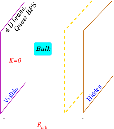
Figure 1: Schematic representation of the old ekpyrotic model as a bulk – boundary branes in an effective five dimensional theory. Our Universe is to be identified with the visible brane, and a bulk brane is spontaneously nucleated near the hidden brane, moving towards our universe to produce the Big-Bang singularity and primordial perturbations. In the new ekpyrotic scenario, the bulk brane is absent and it is the hidden brane that collides with the visible one, generating the hot Big Bang singularity.

In the “old” scenario ekp , the five dimensional bulk is also assumed to contain various fields not described here, whose excitations can lead to the spontaneous nucleation of yet another, much lighter, freely moving, brane. In the so-called “new” scenario ekpN , and its cyclic extension cyclic , it is the hidden boundary brane that is able to move in the bulk. In both cases, this extra brane, if assumed BPS (as demanded by minimization of the action) is flat, parallel to the boundary branes and initially at rest. Non perturbative effects yield an interaction potential between the visible and the bulk brane. The distance of the former to the latter can be regarded as a scalar field living on the four dimensional visible boundary brane whose effective action is thus that of four dimensional GR together with a scalar field $\varphi$ evolving in an exponential potential, namely

$${\cal S}_{{}_{4}}=\int_{{\cal M}_{4}}\mbox{d}^{4}x\sqrt{-g_{{}_{4}}}\left[{R_{{}_{(4)}}\over 2\kappa}-{1\over 2}\left(\partial\phi\right)^{2}-V(\phi)\right],$$ (2)

with

$$V(\varphi)=-V_{\rm i}\exp\biggr{[}-\frac{4\sqrt{\pi\gamma}}{m_{{}_{\rm Pl}}}(\varphi-\varphi_{\rm i})\biggr{]},$$ (3)

where $\gamma$ is a constant and $\kappa=8\pi G=8\pi/m_{{}_{\rm Pl}}^{2}$. Apart from the sign, the potential is the one that leads to the well known power-law inflation model if the value of $\gamma$ lies in a given range powerlaw .

The interaction between the two branes results in one (bulk or hidden) brane moving towards the other (visible) boundary until they collide. This impact time is then identified with the Big-Bang of standard cosmology. Slightly before that time, the exponential potential abruptly goes to zero so the boundary brane is led to a singular transition at which the kinetic energy of the bulk brane is converted into radiation. The result is, from this point on, exactly similar to standard big bang cosmology, with the difference that the flatness problem is claimed to be solved by saying our Universe originated as a BPS state (see however cyclic ).

Figure 2: Scale factor in the new ekpyrotic scenario. The Universe starts its evolution with a slow contraction phase $a\propto(-\eta)^{1+\beta}$ with $\beta=-0.9$ on the figure. The bounce itself is explicitly associated with a singularity which is approached by the scalar field kinetic term domination phase, and the expansion then connects to the standard Big-Bang radiation dominated phase.

III Cosmological Perturbations in the New Ekpyrotic Model

III.1 The background

As mentioned above, although the physics which describes the evolution and the collision of the branes is very complicated, it is assumed that it can be described by means of a simple four-dimensional model. In this case, the equations that govern the system are nothing but the Einstein equations

$$\frac{3}{a^{2}}\biggl{[}\biggl{(}\frac{a^{\prime}}{a}\biggr{)}^{2}+{\cal K}\biggr{]} = \kappa\rho,$$ (4)

$$-\frac{1}{a^{2}}\biggl{[}2\biggl{(}\frac{a^{\prime}}{a}\biggr{)}^{\prime}+\biggl{(}\frac{a^{\prime}}{a}\biggr{)}^{2}+{\cal K}\biggr{]} = \kappa p,$$ (5)

where a prime denotes a derivative with respect to the conformal time $\eta$. The Hubble parameter can be expressed as $H={\cal H}/a$ where ${\cal H}\equiv a^{\prime}/a$. The equation of state $\omega$ can always be written as

$$\omega\equiv\displaystyle{p\over\rho}=\frac{2\Gamma}{3}\biggl{(}1+\frac{{\cal K}}{{\cal H}^{2}}\biggr{)}^{-1}-1,$$ (6)

where the function $\Gamma(\eta)$ is defined by

$$\Gamma\equiv 1-\frac{{\cal H}^{\prime}}{{\cal H}^{2}}+\frac{{\cal K}}{{\cal H}^{2}}.$$ (7)

This last function is a direct generalization of the quantity $\gamma\equiv 1-{\cal H}^{\prime}/{\cal H}^{2}$ for non spatially flat universes since it gives zero in the case of de Sitter spacetime. In the case of spatially flat sections, the equation of state becomes $\omega=2\gamma/3-1$. For a constant equation of state, the function $\Gamma$ or $\gamma$ are constant. This is the case for the potential (3) and the function $\gamma$ gets a constant value, explaining why we used the same symbol to denote these a priori different objects. For the equation of state $\omega=-1$ (i.e., de Sitter space-time), they vanish. Finally, the sound velocity can be formally defined as

$$c_{{}_{\rm S}}^{2}\equiv p^{\prime}/\rho^{\prime}.$$ (8)

As already mentioned, in the ekpyrotic universe, it is assumed that ${\cal K}=0$. As explained above, the pre-impact phase consists in a scalar field dominated era and an hydrodynamical era. We will follow in details the evolution of the perturbations during these two eras.

III.2 The scalar field era

Let us start with the scalar field era. It is assumed that the evolution of the four-dimensional background is governed by the scalar field potential of Eq. (3). This is a well-studied case and the resolution of the Einstein equations leads to a solution where the scale factor is a power-law of the conformal time

$$a(\eta) = \ell_{0}(-\eta)^{1+\beta},$$ (9)

$$\varphi(\eta) = \varphi_{\rm i}+\frac{m_{{}_{\rm Pl}}}{2}\sqrt{\frac{\gamma}{\pi}}(1+\beta)\ln(-\eta).$$ (10)

As already mentioned, the function $\gamma$ is constant and its value reads $\gamma=(2+\beta)/(1+\beta)$. In the ekpyrotic scenario, one has $0<\beta+1\ll 1$. Since the Hubble parameter is given by $aH=(1+\beta)/\eta<0$, this corresponds to a very slow contraction.

In the case where a single scalar field dominates, the evolution of density perturbations can be described by means of a single equation,

$$\mu^{\prime\prime}+\biggl{[}k^{2}-\frac{(a\sqrt{\gamma})^{\prime\prime}}{a\sqrt{\gamma}}\biggr{]}\mu=0,$$ (11)

where $k$ is the comoving dimensionless wavenumber and the quantity $\mu$ is related to the Bardeen potential Fourier component $\Phi$ by the following relationship

$$\Phi=\frac{{\cal H}\gamma}{2k^{2}}\biggl{(}\frac{\mu}{a\sqrt{\gamma}}\biggr{)}^{\prime}.$$ (12)

These quantities are related to the functions $v$ and $z$ in Eqs. (19) and (21) of Ref. perturbekp through $v\propto\mu$ and $z\propto a\sqrt{\gamma}$. The initial condition for the function $\mu$ are fixed by the assumption that the quantum fluctuations are initially placed in the vacuum state. This amounts to

$$\lim_{k/(aH)\rightarrow+\infty}\mu=-\frac{4\sqrt{\pi}}{m_{{}_{\rm Pl}}}\frac{{\rm e}^{-ik(\eta-\eta_{\rm i})}}{\sqrt{2k}}.$$ (13)

For a power-law scale factor, the equation of motion for the quantity $\mu$ can be solved exactly in terms of Bessel functions as $\mu=(k\eta)^{1/2}\left[A_{1}(k)J_{\beta+1/2}(k\eta)+A_{2}(k)J_{-(\beta+1/2)}(k\eta)\right]$. In this case, the Bardeen potential can be written as

$$\Phi(\eta)=-\frac{{\cal H}\sqrt{\gamma}}{2ka}(k\eta)^{1/2}\biggl{[}A_{1}(k)J_{\beta+3/2}(k\eta)-A_{2}(k)J_{-(\beta+3/2)}(k\eta)\biggr{]},$$ (14)

where the coefficients $A_{1}(k)$ and $A_{2}(k)$ are given by

$$A_{1}(k) = \frac{\pi\sqrt{8}}{m_{{}_{\rm Pl}}\cos\beta\pi}\frac{{\rm e}^{i(k\eta_{\rm i}-\pi\beta/2)}}{\sqrt{2k}},$$ (15)

$$A_{2}(k) = -iA_{1}{\rm e}^{i\pi\beta}.$$ (16)

Although these formulas are exact, there are not so easy to work with and their interpretation is not especially illuminating. In order to facilitate the interpretation, it is interesting to proceed as follows. In the general case, i.e., even if the scale factor does not behave as a power-law of the conformal time, the quantity $\mu$ can be expressed as

$$\mu(\eta)=\sum_{n=0}^{\infty}b_{2n}(\eta)k^{2n},$$ (17)

where the coefficients $b_{2n}(\eta)$ can be found by plugging the previous equation in the equation of motion for $\mu$ and by identifying the corresponding order in $k$. One finds

$$\mu(\eta) = \bar{A}_{1}a\sqrt{\gamma}\biggl{[}1-k^{2}\int^{\eta}\frac{{\rm d}\tau}{(a^{2}\gamma)(\tau)}\int^{\tau}{\rm d}\tau^{\prime}(a^{2}\gamma)(\tau^{\prime})+{\cal O}(k^{4})\biggr{]}$$ (18)

$$+\bar{A}_{2}a\sqrt{\gamma}\int^{\eta}\frac{{\rm d}\tau}{(a^{2}\gamma)(\tau)}\biggl{[}1-k^{2}\int^{\tau}{\rm d}\tau^{\prime}(a^{2}\gamma)(\tau^{\prime})\int^{\tau^{\prime}}\frac{{\rm d}\tau^{\prime\prime}}{(a^{2}\gamma)(\tau^{\prime\prime})}+{\cal O}(k^{4})\biggr{]}.$$

Inserting this expansion into the expression of $\Phi$, one obtains at leading order

$$\Phi(\eta)=\frac{\bar{A}_{2}(k)}{2k^{2}}\frac{{\cal H}}{a^{2}}-\frac{\bar{A}_{1}(k)}{2}\frac{{\cal H}}{a^{2}}\int^{\eta}{\rm d}\tau a^{2}\gamma.$$ (19)

It is necessary to push the expansion to second order because we see that the first term of $[\mu/(a\sqrt{\gamma})]^{\prime}$ vanishes in the expression of the Bardeen potential. Notice that Eq. (22) of Ref. perturbekp is not correct since one integration is missing, see Eq. (18). The fact that it is necessary to push the expansion up to second order to obtain the first non-vanishing term in the Bardeen potential (the same is true for the quantity $\zeta$, see below) has been called a subtlety in Ref. perturbekp whereas this fact has been known for a long time in the literature, see Ref. perturb ; MS . One can easily check that taking the limit $k\eta\rightarrow 0$ in Eq. (14) leads to the same dependence in conformal time as in the previous equation. Explicitly, one has

$$\Phi(\eta)=-\frac{\bar{A}_{2}(k)}{2k^{2}}\frac{1+\beta}{\ell_{0}^{2}}(-\eta)^{-3-2\beta}-\frac{\bar{A}_{1}(k)}{2}\frac{2+\beta}{3+2\beta}.$$ (20)

In an inflationary universe where $\beta\simeq-2$, the $\bar{A}_{1}$-constant mode is the dominant mode since the $\bar{A}_{2}$-mode decays as $-\eta$ when $\eta\rightarrow 0$. The fact that it is proportional to $\beta+2$ and therefore vanishes when $\beta=-2$ is just the well-known fact that there is no density perturbations at all in a pure de Sitter phase. In the ekpyrotic case, the situation is exactly the opposite, i.e., the $\bar{A}_{1}$-constant mode is no longer the dominant mode. The dominant mode is now the $\bar{A}_{2}$-mode since this one scales like $-1/\eta$. The important point is the $k$-dependence of this mode. This can be found by comparing the exact equation (14) with Eq. (19) which allows us to make the link between the constants $\bar{A}_{1}$, $\bar{A}_{2}$ and $A_{1}$, $A_{2}$. One obtains

$$\frac{\bar{A}_{2}(k)}{k^{2}}\sim k^{-\beta-5/2},\quad\bar{A}_{1}(k)\sim k^{\beta+1/2}.$$ (21)

Therefore, for $\beta\simeq-1$, the dominant mode acquires a scale invariant spectrum since $\Phi\propto k^{-3/2}$. Note however in that respect that the ekpyrotic and de Sitter cases are already at this stage very different since in the de Sitter case, the scale invariant part of the spectrum is time independent, contrary to what happens in the ekpyrotic situation.

III.3 The hydrodynamical era

As the bulk brane is approaching the visible brane, the scalar field blows up. In the ekpyrotic scenario, it is assumed that the shape of the potential changes and goes to zero as the collision is taking place. Consequently, just before the collision, the equation of state tends toward a stiff equation of state, i.e., $\omega_{0}=1$. More generally, Ref. perturbekp considers the situation where

$$\omega\equiv{p\over\rho}=\omega_{0}+\omega_{1}\eta+\omega_{2}\eta^{2}+\cdots.$$ (22)

Being given a general equation of state $\omega(\eta)$, it is easy to find the corresponding scale factor. It reads

$$a(\eta)=\ell_{0}\exp\biggl{(}\int^{\eta}{\rm d}\tau\biggl{\{}C+\frac{1}{2}\int^{\tau}{\rm d}\tau^{\prime}[1+3\omega(\tau^{\prime})]\biggr{\}}^{-1}\biggr{)},$$ (23)

where $\ell_{0}$ and $C$ are arbitrary constants. In this article, without any essential loss of generality, we restrict our considerations to the truncated equation of state $\omega=1+\omega_{1}\eta$, i.e., $\omega_{0}=1$. In this case the scale factor can be integrated explicitly using Eq. (2.154) of Ref. Grad and the result reads

$$a(\eta)=\ell_{0}\left|\frac{\eta}{2(1+3\omega_{0})+3\omega_{1}\eta}\right|^{2/(1+3\omega_{0})}.$$ (24)

To our knowledge, this is a new solution. Moreover, as we will show, all the relevant perturbed quantities can be calculated exactly in this model. Therefore, this also constitutes a new exactly integrable case for the theory of cosmological perturbations. In the previous formula the constant $C$ has been chosen such that $a(0)=0$ in agreement with the new ekpyrotic scenario. There is a divergence when $\omega_{1}\eta=-8/3$. This just signals that more terms should be included in the Taylor series of the equation of state which anyway, under the form of Eq. (22), is only valid for in the vicinity of the bounce. Moreover, in the collapsing phase, one has $\omega_{1}<0$ with $\eta<0$ so the model is divergence free in the pre impact era. It is interesting to see how the physical quantities that characterize the model behave. We find

$${\cal H}(\eta) = \frac{4}{\eta(8+3\omega_{1}\eta)},$$ (25)

$$\kappa\rho(\eta) = \frac{48}{\ell_{0}^{2}|\eta^{3}(8+3\omega_{1}\eta)|},$$ (26)

$$c_{{}_{\rm S}}^{2}(\eta) = \frac{5}{6}+\frac{3}{4}\omega_{1}\eta+\frac{1}{6+3\omega_{1}\eta},$$ (27)

where the “sound velocity” is given by Eq. (8). As expected, the Hubble parameter and the energy density blow up at $\eta=0$. These functions are shown in Fig. 3

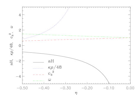
Figure 3: Characteristic functions of the new ekpyrotic model [See Eqs. (22), (25), (26) and (27)]. The parameters are chosen as $\ell_{0}=1$ and $\omega_{1}=-1$ (the ekpyrotic scenario requires $\omega_{1}$ to be negative).

On the contrary, the equation of state and the sound velocity are regular. The fact that the sound velocity is $1$ at $\eta=0$ can easily be understood. This is a consequence of the equation

$$\omega^{\prime}=-3{\cal H}(c_{{}_{\rm S}}^{2}-\omega)(1+\omega).$$ (28)

When $\eta\to 0$ and $\omega\not=-1$, it is necessary that $c_{{}_{\rm S}}^{2}$ behaves as $c_{{}_{\rm S}}^{2}\to\omega$ in order to obtain a finite $\omega^{\prime}$ as ${\cal H}$ diverges in this limit.

In the phase dominated by an (effective) hydrodynamical fluid, the equation that governs the evolution of density perturbations reads

$$\Phi^{\prime\prime}+3(1+c_{{}_{\rm S}}^{2}){\cal H}\Phi^{\prime}+[2{\cal H}^{\prime}+(1+3c_{{}_{\rm S}}^{2})({\cal H}^{2}-{\cal K})]\Phi+c_{{}_{\rm S}}^{2}(k^{2}-{\cal K})\Phi=0,$$ (29)

where we have assumed that there is no entropy production. This equation can also be put under the form of an equation of motion for a parametric oscillator. Let us define $\mu$ and $\theta$ by

$$\mu\equiv\frac{2a^{2}\theta}{3{\cal H}}\Phi,\quad\theta\equiv\frac{1}{a}\biggl{(}\frac{\rho}{\rho+p}\biggr{)}^{1/2}\biggl{(}1-\frac{3{\cal K}}{\kappa\rho a^{2}}\biggr{)}^{1/2}=\frac{1}{a}\sqrt{\frac{3}{2\Gamma}},$$ (30)

where $\Gamma$ is defined through Eq. (7). Of course, in the ekpyrotic case, these equations should be used with ${\cal K}=0$, although we wrote them here in their full generality since we will use them in the regular ${\cal K}=1$ case in the following section. Then, the equation of motion of $\mu$ can be written under the form of a parametric oscillator equation of motion

$$\mu^{\prime\prime}+\biggl{[}c_{{}_{\rm S}}^{2}(k^{2}-{\cal K})-\frac{\theta^{\prime\prime}}{\theta}\biggr{]}\mu=0.$$ (31)

As for the scalar field case, one can solve this equation perturbatively. The solution now reads

$$\mu(\eta) = B_{1}(k)\theta\biggl{[}1-k^{2}\int^{\eta}\frac{{\rm d}\tau}{\theta^{2}(\tau)}\int^{\tau}{\rm d}\tau^{\prime}(c_{{}_{\rm S}}^{2}\theta^{2})(\tau^{\prime})+{\cal O}(k^{4})\biggr{]}$$ (32)

$$+B_{2}(k)\theta\int^{\eta}\frac{{\rm d}\tau}{\theta^{2}}\biggl{[}1-k^{2}\int^{\tau}{\rm d}\tau^{\prime}(c_{{}_{\rm S}}^{2}\theta^{2})(\tau^{\prime})\int^{\tau^{\prime}}\frac{{\rm d}\tau^{\prime\prime}}{\theta^{2}(\tau^{\prime\prime})}+{\cal O}(k^{4})\biggr{]}.$$

In the long-wavelength approximation, the solution is

$$\Phi=\frac{3}{2}B_{1}(k)\frac{{\cal H}}{a^{2}}+\frac{3}{2}B_{2}(k)\frac{{\cal H}}{a^{2}}\int^{\eta}\frac{{\rm d}\tau}{\theta^{2}}.$$ (33)

As expected, at this order, the solution does not depend on the sound velocity. In the above equation, the integral can be easily performed. The Bardeen potential reads

$$\Phi(\eta)=\frac{6sB_{1}(k)}{\ell_{0}^{2}\eta^{2}}+\frac{B_{2}(k)}{9(\omega_{1}\eta)^{2}}[-12\omega_{1}\eta+9(\omega_{1}\eta)^{2}+32\ln(8+3\omega_{1}\eta)],$$ (34)

where $s$ is the sign of the conformal time $\eta$. The Bardeen potential blows up as $\eta$ is approaching zero and the linear theory becomes meaningless. In Ref. perturbekp , it is argued that $\Phi(\eta)$ should not be used. Instead, it is proposed to use the density contrast Bardeen $\epsilon_{{}_{\rm m}}\equiv\delta\rho/\rho$ which is linked to the Bardeen potential by the relation

$$\epsilon_{{}_{\rm m}}=\frac{k^{2}\Phi}{\rho a^{2}}.$$ (35)

Then the superhorizon solution of $\epsilon_{\rm m}$ can be expressed as

$$\epsilon_{{}_{\rm m}}=\frac{k^{2}B_{1}(k)}{2{\cal H}a^{2}}+\frac{k^{2}B_{2}(k)}{2{\cal H}a^{2}}\int^{\eta}\frac{{\rm d}\tau}{\theta^{2}}.$$ (36)

Explicitly, the solution can be written as

$$\epsilon_{{}_{\rm m}}=\frac{8k^{2}sB_{1}(k)}{\ell_{0}^{2}}\left[1+\frac{3}{4}\omega_{1}\eta+\frac{9}{64}(\omega_{1}\eta)^{2}\right]+\frac{4k^{2}B_{2}(k)}{27\omega_{1}^{2}}\left[-12\omega_{1}\eta+9(\omega_{1}\eta)^{2}+32\ln(8+3\omega_{1}\eta)\right]\left[1+\frac{3}{4}\omega_{1}\eta+\frac{9}{64}(\omega_{1}\eta)^{2}\right],$$ (37)

in which the limit $\omega_{1}\to 0$, being singular, is not applicable. We see that the variable $\epsilon_{{}_{\rm m}}$ is regular at $\eta=0$ because the divergence has been canceled by the factor $1/(\rho a^{2})$. Note however that for a constant equation of state $\omega=\omega_{0}$, this variable is not regular if $-1/3\leq\omega_{0}<1$. The regularity of $\epsilon_{{}_{\rm m}}$ thus depends on the matter content as the singularity is approached. If we expand the above equation around $\eta=0$, we find

$$\epsilon_{{}_{\rm m}}=\biggl{[}\frac{8k^{2}sB_{1}}{\ell_{0}^{2}}+\frac{128k^{2}B_{2}}{9\omega_{1}^{2}}\ln 2\biggr{]}\biggl{[}1+\frac{3}{4}\omega_{1}\eta+{\cal O}(\eta^{3})\biggr{]}+\biggl{[}\frac{9k^{2}sB_{1}\omega_{1}^{2}}{8\ell_{0}^{2}}+k^{2}B_{2}\left(1+2\ln 2\right)\biggr{]}\biggr{[}\eta^{2}+{\cal O}(\eta^{3})\biggr{]}.$$ (38)

This equation is in agreement with Eq. (42) of Ref. perturbekp with $\omega_{2}=0$. For $k\not=0$, the first ${\cal O}(\eta^{3})$ is replaced with ${\cal O}(k^{2}\eta^{2}\ln|\eta|)$. The Bardeen potential and the density contrast are plotted in Fig. 4.

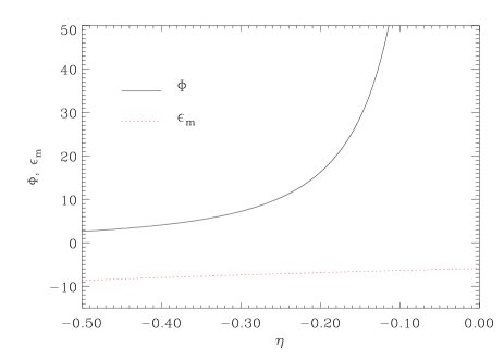
Figure 4: The divergence in the Bardeen potential and the gauge invariant energy density perturbation near the bounce in the new ekpyrotic scenario. Parameters are chosen as $\ell_{0}=1$ and $\omega_{1}=-1$. The Bardeen potential $\Phi$ is from Eq. (34) with $sB_{1}=B_{2}=1$, while $k^{2}sB_{1}=k^{2}B_{2}=1$ for $\epsilon_{{}_{\rm m}}$ in Eq. (37).

In Ref. perturbekp , the solution $\epsilon_{{}_{\rm m}}$ has not been expanded in the basis of the growing and decaying mode but has been written as

$$\epsilon_{{}_{\rm m}}=\epsilon_{0}(k)D(k,\eta)+\epsilon_{2}(k)E(k,\eta),$$ (39)

where $D\equiv 1+3\omega_{1}\eta/4+{\cal O}(k^{2}\eta^{2}\ln|\eta|)$ and $E\equiv\eta^{2}+{\cal O}(\eta^{3})$. The link between the coefficients of the growing and decaying modes $B_{1}$, $B_{2}$ and the coefficients $\epsilon_{0}$ and $\epsilon_{2}$ of the $(D,E)$ basis is obvious

$$\epsilon_{0}(k) = \frac{8k^{2}sB_{1}}{\ell_{0}^{2}}+\frac{128k^{2}B_{2}}{9\omega_{1}^{2}}\ln 2,$$ (40)

$$\epsilon_{2}(k) = \frac{9k^{2}sB_{1}\omega_{1}^{2}}{8\ell_{0}^{2}}+k^{2}B_{2}\left(1+2\ln 2\right).$$ (41)

At leading order in $k$, the previous equations imply $\epsilon_{2}=3\epsilon_{0}w^{(2)}/8$, in agreement with the equation in the last line of the paragraph below Eq. (45) of Ref. perturbekp , being given that in the present context the variable $w^{(2)}$ of Ref. perturbekp is simply $3\omega_{1}^{2}/8$; this means that $\epsilon_{0}$ and $\epsilon_{2}$ are of the same order in $k$. The inverse transformation reads

$$sB_{1}(k) = \frac{\ell_{0}^{2}}{8k^{2}}\left(1+2\ln 2\right)\epsilon_{0}-\frac{16\ell_{0}^{2}\ln 2}{9\omega_{1}^{2}k^{2}}\epsilon_{2},$$ (42)

$$B_{2}(k) = \frac{1}{k^{2}}\biggl{(}-\frac{9\omega_{1}^{2}}{64}\epsilon_{0}+\epsilon_{2}\biggr{)}.$$ (43)

Let us notice that if we want to obtain the other terms of the expansion, we need to use the higher order terms in the expression (32) of $\mu(\eta)$. For example the first (respectively second) branch next-to-leading order term can be expressed in terms of elementary functions and of dilogarithm Li${}_{2}(\eta)$ [resp. trilogarithm Li${}_{3}(\eta)$] functions dilog . An expansion of these functions around $\eta=0$ reproduces Eq. (43) of Ref. perturbekp .

Finally, let us end this section by a discussion on the quantity $\zeta(\eta)$. This one is defined by the following equation

$$\zeta \equiv \frac{2}{3}\frac{{\cal H}^{-1}\Phi^{\prime}+\Phi}{1+\omega}+\Phi$$ (44)

$$= \frac{{\cal H}^{2}+{\cal K}}{{\cal H}^{2}}\theta^{2}\biggl{(}\frac{\mu}{\theta}\biggr{)}^{\prime}+\frac{3{\cal H}\mu}{2a^{2}\theta}\biggl{[}1-\frac{\gamma}{\Gamma}\biggl{(}1+\frac{{\cal K}}{{\cal H}^{2}}\biggl{)}\biggr{]}.\$$ (45)

Let us briefly recall under which conditions, the quantity $\zeta$ can be considered as a constant. First of all, ${\cal K}$ should be equal to zero such that the last term in the above equation disappears. Secondly, there should be no entropy perturbations. Thirdly, only the growing mode should be considered and we note that it is crucial to discard the singular mode MS . In order to obtain the explicit expression of $\zeta$, one can insert the formula (32) giving $\mu$ in Eq. (45). As is well known MS , it is necessary to push the expansion to second order because we see that the first term of $(\mu/\theta)^{\prime}$ vanishes. One obtains

$$\zeta=-B_{1}k^{2}\int^{\eta}{\rm d}\tau c_{{}_{\rm S}}^{2}(\tau)\theta^{2}(\tau)+B_{2}+{\cal O}(k^{2}).$$ (46)

For the exact model studied here the integral in the above equation can be performed exactly. The result reads

$$\zeta=-\frac{k^{2}sB_{1}}{12\ell_{0}^{2}}\biggl{[}27\omega_{1}\eta+\frac{4}{2+\omega_{1}\eta}+48\ln(-\eta)\biggr{]}+B_{2}.$$ (47)

Therefore, this quantity has a logarithmic divergence as the point where the scale factor vanishes is approached. This is in agreement with the analysis of Ref. perturbekp . The divergence is again a signal that the linear theory looses any meaning.

III.4 Matching conditions

We have at our disposal the solutions in each era. The goal is now to join them. The first step is to pass from the scalar field era to the hydrodynamical era. Since the equation of state can be made continuous at this point, one has $[a]=[a^{\prime}]=[a^{\prime\prime}]=0$. In this case, the usual joining conditions can be used and the Bardeen potential and its derivative are continuous. This means that the growing mode in the hydrodynamical era acquires a scale invariant spectrum. In other words, $B_{1}(k)\sim k^{-3/2}$ and $B_{2}\sim k^{-1/2}$ because $\Phi$ has the same shape in both eras. The same applies to the other transition, in the expanding regime, from domination by the scalar field kinetic term to the radiation epoch.

Clearly, the non trivial step is how to propagate the perturbations through the singularity. We have to connect the solution in the pre-impact hydrodynamical phase with equation of state $\omega=1+\omega_{1}^{<}\eta$ with the solution in the post-impact phase with $\omega=1+\omega_{1}^{>}\eta$, being given that $\omega_{1}^{<}\neq\omega_{1}^{>}$. A priori, this seems simply impossible because the theory (a fortiori the linear theory) looses any meaning (signaled by the divergence of the scalar curvature and/or of the Bardeen potential): how to perturb around a singular background? Even if we are ready to accept this, the theory suffers from a serious trans-Planckian problem since all the wavelengths become at some point smaller than the Planck length transPl . However, despite these seemingly insurmountable difficulties, Ref. perturbekp goes on along the following lines. The fact that the quantity $\epsilon_{{}_{\rm m}}$ is regular is used in an essential way. A first approach would be to impose $[\epsilon_{{}_{\rm m}}]=[\epsilon_{{}_{\rm m}}^{\prime}]=0$. The first condition means $\epsilon_{0}^{>}=\epsilon_{0}^{<}$ whereas the second cannot be applied since $\epsilon_{{}_{\rm m}}^{\prime}(0)=3\omega_{1}/4$, which is required to be different in the pre- and post impact eras since $\omega_{1}^{<}\neq\omega_{1}^{>}$. The fact that the derivative cannot be made continuous (contrary to the claims of Ref. perturbekp ) can be directly traced back to the fact that the background is singular. As a consequence, one cannot find $\epsilon_{2}^{>}$. Then, a new suggestion is given to find the coefficients $\epsilon_{0}^{>}$ and $\epsilon_{2}^{>}$. It consists in assuming that

$$\epsilon_{0}^{>}(k)=\epsilon_{0}^{<}(k),\qquad\epsilon_{2}^{>}(k)=\epsilon_{2}^{<}(k),$$ (48)

i.e., one assumes that the energy density perturbation as well as the second derivative of $(\epsilon_{{}_{\rm m}}-\epsilon_{0}D)$ are continuous across the bounce. At this point, we would like to stress the following remark: the usual matching conditions stem from a well defined geometrical requirement MS ; matching . In physics, in general, the requirement is made that the function and its derivative should be continuous because the point considered is almost never considered to be a singular point. The situation here is therefore extremely special as there does not appear to be any physical reason to enforce any matching conditions, especially on a variable which, although finite, is the perturbation of a diverging background quantity. Let us however press on to assert if they lead, as claimed in Ref. perturbekp , to a unique spectrum: this fact in itself would maybe justify a posteriori this choice for the criterion.

Of course, in the post-impact phase, one is interested in the coefficient of the growing mode, i.e., in the spectrum of $\Phi$ perturbations, and not in the coefficients $\epsilon_{0}^{>}$ and $\epsilon_{2}^{>}$. This is because the growing mode directly provides us with the spectrum. Plugging Eqs. (40) and (41) into Eq. (43), and using the continuity condition (48) permits to evaluate this spectrum. The result reads

$$B_{1}^{>}(k) = -B_{1}^{<}(k)\left[1+2\left(1-\frac{\omega_{1}^{<2}}{\omega_{1}^{>2}}\right)\ln 2\right]+\frac{16\ell_{0}^{2}\ln 2}{9}B_{2}^{<}(k)(1+2\ln 2)\left({1\over\omega_{1}^{<2}}-{1\over\omega_{1}^{>2}}\right).$$ (49)

$$B_{2}^{>}(k) = -\frac{9}{8\ell_{0}^{2}}B_{1}^{<}(k)(\omega_{1}^{<2}-\omega_{1}^{>2})+B_{2}^{<}(k)\left[1+2\left(1-\frac{\omega_{1}^{>2}}{\omega_{1}^{<2}}\right)\ln 2\right].$$ (50)

Therefore, in the limit of long wavelengths, the dominant term is $B_{1}^{<}(k)$ and we have $B_{2}^{>}(k)\sim k^{-3/2}$ at least as long as $\omega_{1}^{<2}\neq\omega_{1}^{>2}$. In this case, the spectrum of the Bardeen potential is scale-invariant in the post-impact phase. Let us now study the new prescription in greater details. It is clear that the function $\epsilon_{{}_{\rm m}}$ can also be written as

$$\epsilon_{{}_{\rm m}} = \epsilon_{0}(k)D(k,\eta)+\frac{\epsilon_{2}(k)}{f(\omega_{1},k)}f(\omega_{1},k)E(k,\eta),$$ (51)

$$= \bar{\epsilon}_{0}(k)\bar{D}(k,\eta)+\bar{\epsilon}_{2}(k)\bar{E}(k,\eta),$$ (52)

where $\bar{\epsilon}_{0}(k)=\epsilon_{0}(k)$, $\bar{D}(k,\eta)=D(k,\eta)$, $\bar{\epsilon}_{2}(k)=\epsilon_{2}(k)/f(\omega_{1},k)$ and $\bar{E}(k,\eta)=f(\omega_{1},k)E(k,\eta)$. Of course the choice of the basis has no physical meaning at all and we can equally well expand $\epsilon_{{}_{\rm m}}(\eta)$ in the basis $(D,E)$ or $(\bar{D},\bar{E})$. Let us remark that we could choose a more general change of basis but in the present context the continuity of $\epsilon_{{}_{\rm m}}$ would no longer be guaranteed. In the standard case, such a change of basis has obviously no consequence on the final spectrum as it should. As we are going to show, this is not the case for the new proposal of Ref. perturbekp . With the new basis, the matching conditions of Eq. (48) transforms into

$$\bar{\epsilon}_{0}^{>}(k)=\bar{\epsilon}_{0}^{<}(k),\qquad\bar{\epsilon}_{2}^{>}(k)=\bar{\epsilon}_{2}^{<}(k).$$ (53)

This leads to the following expression for the coefficient $B_{2}^{>}(k)$

$$B_{2}^{>}(k)=-\frac{9}{8\ell_{0}^{2}}B_{1}^{<}(k)\left(\frac{f^{>}}{f^{<}}\omega_{1}^{<2}-\omega_{1}^{>2}\right)+B_{2}^{<}(k)\left[\frac{f^{>}}{f^{<}}+2\left(\frac{f^{>}}{f^{<}}-\frac{\omega_{1}^{>2}}{\omega_{1}^{<2}}\right)\ln 2\right].$$ (54)

Now since the choice of $f$ is completely arbitrary, one can always choose $f^{>}=\omega_{1}^{>2}$ and $f^{<}=\omega_{1}^{<2}$. In this case the first term cancels out and we are left with a spectrum $B_{2}^{>}(k)\sim k^{-1/2}$ corresponding to a spectral index $n_{{}_{\rm S}}=3$. More generally, one is free to choose the function $f$ as a function of $k$ and in this case the spectrum is also completely changed.

In conclusion, the proposal of Ref. perturbekp rests on a non-physical choice. Choosing the normalization of the function $E$ such that it leads to a scale invariant spectrum seems to be arbitrary. The standard junction conditions do not depend on the normalization of the mode functions. So even if one admits that we can somehow pass through a singularity, it seems that there is no convincing way to find a scale-invariant spectrum. This is probably because through a singularity any result can be obtained.

III.5 Testing the matching conditions: the radiation to matter transition

In a recent proposal Ruth , it was argued that the junction conditions advocated in the previous section could be expressed in a very similar way to the usual junction conditions. It is well-known mtw that matching conditions follow from the requirement that $[h_{ij}]=0$ and $[K_{ij}]=0$ where $h_{ij}$ is the metric of the spacelike sections and $K_{ij}$ is the associated second fundamental form. The question is then: on which surface should these conditions be imposed? The standard answer is to match on a surface of constant longitudinal gauge (gauge-invariant) energy density denoted $\epsilon_{\rm g}$ by Bardeen Bardeen . The proposal of Ref. Ruth is to perform the matching on a surface of constant comoving (gauge-invariant) energy density denoted $\epsilon_{\rm m}$. This is the quantity used above and advocated in perturbekp .

The standard junction conditions reduce to the continuity of the Bardeen potential and $\zeta$, $[\Phi]=[\zeta]=0$. The new ones amount to $[\Phi]=[{\cal H}\Phi+\Phi^{\prime}]=0$; see Eqs. (20) and (21) of Ref. Ruth . We have taken the surface layer pressure to be zero as it was argued in Ref. Ruth that this does not play a crucial role in the present context. However, we will come back to this point shortly. If $[a]=[a^{\prime}]=[a^{\prime\prime}]=0$, the two sets of conditions are equivalent and both lead to $[\Phi]=[\Phi^{\prime}]=0$ as already mentioned. On the other hand, there exists a situation for which the two sets are not equivalent, namely that of a sharp transition, i.e., one for which the equation of state $\omega$ jumps. In order to discuss the accuracy of the new proposal, let us examine the case of the radiation to matter transition. The advantage is that the exact solution is known and then we can compare whether the different set of junction conditions reproduce or not the correct result.

In the radiation to matter domination transition, Einstein equations can be solved exactly and the scale factor is given by the following expression perturb

$$a(\eta)=a_{\rm eq}\biggl{[}b^{2}\biggl{(}\frac{\eta}{\eta_{\rm eq}}\biggr{)}^{2}+2b\biggl{(}\frac{\eta}{\eta_{\rm eq}}\biggr{)}\biggr{]}.$$ (55)

For $\eta\ll\eta_{\rm eq}$, the scale factor is approximatively linear in the conformal time and the universe is radiation dominated whereas for $\eta\gg\eta_{\rm eq}$ it is quadratic in the conformal time and the universe is matter dominated. The freely adjustable coefficient $b=\sqrt{2}-1$ is chosen such that $a(\eta=\eta_{\rm eq})=a_{\rm eq}$ (note that the different choice $b=1$ is made in perturb ). The superhorizon solution for the Bardeen potential is Eq. (33) which, in the case of the radiation-matter transition (55), can be written as

$$\Phi(\eta)=\biggl{(}\frac{3b}{\eta_{\rm eq}a_{\rm eq}^{2}}B_{1}\biggr{)}\frac{b\eta/\eta_{\rm eq}+1}{b^{3}(\eta/\eta_{\rm eq})^{3}(b\eta/\eta_{\rm eq}+2)^{3}}+B_{2}\frac{b\eta/\eta_{\rm eq}+1}{(b\eta/\eta_{\rm eq}+2)^{3}}\biggl{[}\frac{3}{5}b^{2}\biggl{(}\frac{\eta}{\eta_{\rm eq}}\biggr{)}^{2}+3b\biggl{(}\frac{\eta}{\eta_{\rm eq}}\biggr{)}+\frac{13}{3}+\frac{1}{b\eta/\eta_{\rm eq}+1}\biggr{]},$$ (56)

in which the lower bound of the integral in Eq. (33) has been chosen to cancel the ${\cal H}/a^{2}$ contribution of the second branch. From this expression, it is easy to check that, for the growing mode, one has

$$\frac{\Phi(\eta\gg\eta_{\rm eq})}{\Phi(\eta\ll\eta_{\rm eq})}=\frac{9}{10}.$$ (57)

This result is nothing but the standard result of the inflationary cosmology, applied to the radiation to matter transition. In the same manner, the quantity $\zeta$ can be calculated exactly. One obtains

$$\zeta(\eta)=B_{2}.$$ (58)

This result is valid as soon as the decaying mode, not taken into account here, had enough time to decay.

Let us now turn to the piecewise solution for which the same situation can also be described by means of the following approximation for the scale factor

$$a^{<}(\eta) = \frac{a_{\rm eq}}{\eta_{\rm eq}}\eta,$$ (59)

$$a^{>}(\eta) = \frac{a_{\rm eq}}{4}\biggl{(}1+\frac{\eta}{\eta_{\rm eq}}\biggr{)}^{2},$$ (60)

where $[a]=[a^{\prime}]=0$ has been imposed in agreement with the background junction conditions. For each region, the exact superhorizon solution for the Bardeen potential can easily be obtained and reads

$$\Phi^{<}(\eta) = \frac{3B_{1}^{<}}{2\eta_{\rm eq}a_{\rm eq}^{2}}\biggl{(}\frac{\eta}{\eta_{\rm eq}}\biggr{)}^{-3}+\frac{2}{3}B_{2}^{<},$$ (61)

$$\Phi^{>}(\eta) = \frac{48B_{1}^{>}}{\eta_{\rm eq}a_{\rm eq}^{2}}\biggl{(}1+\frac{\eta}{\eta_{\rm eq}}\biggr{)}^{-5}+\frac{3}{5}B_{2}^{>}.$$ (62)

Similarly, one gets the quantity $\zeta$ as

$$\zeta^{<}(\eta)=B_{2}^{<},\quad\zeta^{>}(\eta)=B_{2}^{>},$$ (63)

where, as emphasized above, the decaying mode is assumed negligible.

We are now in the position to relate the various quantities of interest before and after the transition. For this purpose, let us now apply to set of junction conditions. The standard matching conditions stipulate that $[\Phi]=[\zeta]=0$. This amounts to

$$B_{1}^{>} = B_{1}^{<}+\frac{2\eta_{\rm eq}a_{\rm eq}^{2}}{45}B_{2}^{<},$$ (64)

$$B_{2}^{>} = B_{2}^{<}.$$ (65)

For a sharp transition having $[{\cal H}]=0$ and $[a^{\prime\prime}]\not=0$, implying $[p]\not=0$, the matching conditions proposed in Ref. Ruth are equivalent to $[\Phi]=[\Phi^{\prime}]=0$. From the very definition (44) of $\zeta$, these conditions, together with $[\omega]\not=0$, implies $[\zeta]\not=0$. Therefore, as announced, the two sets of junction conditions are not equivalent. Applying the new matching procedure yields

$$B_{1}^{>} = \frac{6}{5}B_{1}^{<},$$ (66)

$$B_{2}^{>} = -\frac{1}{2\eta_{\rm eq}a_{\rm eq}^{2}}B_{1}^{<}+\frac{10}{9}B_{2}^{<}.$$ (67)

In turn, the coefficients $B_{1}^{<}$ and $B_{2}^{<}$ are fixed by the initial conditions at some time $\eta_{\rm i}$. Let us express these coefficients in terms of $\Phi_{\rm i}$ and $\Phi^{\prime}_{\rm i}$, the Bardeen potential and its derivative at some initial time $\eta_{\rm i}\ll\eta_{\rm eq}$ respectively. Before the transition, the result is

$$\Phi^{<}(\eta)=\Phi_{\rm i}+\frac{1}{3}\eta_{\rm i}\Phi_{\rm i}^{\prime}-\frac{1}{3}\eta_{\rm i}\Phi_{\rm i}^{\prime}\frac{\eta_{\rm i}^{3}}{\eta^{3}}.$$ (68)

If one uses the standard junction conditions, the Bardeen potential after the transition can be written as

$$\Phi^{>}(\eta) = \frac{16}{5}\biggl{(}\Phi_{\rm i}+\frac{1}{3}\eta_{\rm i}\Phi_{\rm i}^{\prime}-\frac{10}{3}\eta_{\rm i}\Phi_{\rm i}^{\prime}\frac{\eta_{\rm i}^{3}}{\eta_{\rm eq}^{3}}\biggr{)}\biggl{(}1+\frac{\eta}{\eta_{\rm eq}}\biggr{)}^{-5}$$ (69)

$$+\frac{9}{10}\biggl{(}\Phi_{\rm i}+\frac{1}{3}\eta_{\rm i}\Phi_{\rm i}^{\prime}\biggr{)},$$

leading to the correct ratio as in Eq. (57). On the other hand, the matching conditions proposed in Ref. Ruth lead to

$$\Phi^{>}(\eta) = -\frac{64}{5}\eta_{\rm i}\Phi_{\rm i}^{\prime}\frac{\eta_{\rm i}^{3}}{\eta_{\rm eq}^{3}}\biggl{(}1+\frac{\eta}{\eta_{\rm eq}}\biggr{)}^{-5}+\Phi_{\rm i}$$ (70)

$$+\frac{1}{3}\eta_{\rm i}\Phi_{\rm i}^{\prime}\biggl{(}1+\frac{1}{5}\frac{\eta_{\rm i}^{3}}{\eta_{\rm eq}^{3}}\biggr{)}.$$

The ratio between the constant parts of the Bardeen potential before and after the transition is then very close to unity, namely $\simeq 1+\eta_{\rm i}\Phi_{\rm i}^{\prime}/(3\Phi_{\rm i})$. Fig. 5 illustrates this point.

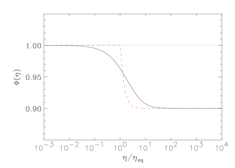
Figure 5: Time evolution of the Bardeen potential during the radiation to matter domination transition. The full line shows the exact solution (56), the dashed line represents the usual approximation (69), and the dotted line is obtained using the new proposal (70) for the junction conditions. This last approximation is not in fact constant but, as discussed below Eq. (70), only hardly varying at all on the scale shown. In order to ensure that initial conditions are identical for the three curves, we have set numerically $\Phi_{\rm i}=\Phi_{\rm i}^{\prime}=1$ [see above Eq. (68)], and used $B_{1}\simeq-b^{2}a^{2}_{\rm eq}\eta_{\rm i}^{4}(b\Phi_{\rm i}+8\eta_{\rm eq}\Phi_{\rm i}^{\prime})/9\eta_{\rm eq}^{2}$ and $B_{2}\simeq 3/2(\Phi_{\rm i}+\eta_{\rm i}\Phi_{\rm i}^{\prime}/3)$ in Eq. (56) valid in the limit $\eta_{\rm i}\ll\eta_{\rm eq}$.

The new proposal does not reproduce the exact result for the radiation to matter domination transition. One could argue however that the situation for which the new junction conditions were suggested is different from the standard case, and that therefore new rules must be applied. This would require different physical prescriptions for different situations, whereas it seems to us that a unified approach is more satisfactory.

IV Hydrodynamical bounce and the conserved quantity $\zeta$

We now turn to the second topic of this work in relation with the bouncing phase. From now on, we shall consider a regular bounce, i.e., one such that the scale factor never vanishes. As already mentioned, it is clear that such a bounce cannot be described in the same framework as in the ekpyrotic case because it is impossible to have a bounce if ${\cal K}=0$ within GR. For instance, this can be seen if matter consists of a single scalar field since Einstein equations yield

$$\rho+p={2\over\kappa a^{2}}({\cal H}^{2}-{\cal H}^{\prime}),$$ (71)

which shows that $\rho+p$ should be negative at the bounce (${\cal H}=0$, ${\cal H}^{\prime}>0$) even though it is positive definite, being also given by $\varphi^{\prime 2}/a^{2}$. Indeed, it is well known that in order to have a bouncing period in a FLRW background, one must violate energy conditions that classical fluids usually do satisfy (as was presented in Ref. ekpN and whose origin can be in fact traced back to Ref. global ). If one insists on having a flat ${\cal K}=0$ situation with, say, a scalar field alone, one must either use other equations, or assume the existence of a singularity.

The only way to have a bounce in GR with a well behaved (NEC preserving) hydrodynamical fluid as the only source of energy momentum is in the case of a closed, ${\cal K}=1$ universe. In this case however, as recently discussed ppnpn1 , one finds that the bounce must be followed by an inflationary epoch, thus considerably lowering the interest of the model as an alternative to inflation. We shall nevertheless study this case as the only fully self-consistent possibility.

In the literature BF ; Hwang , it was suggested to treat the bounce as a GR sharp transition, i.e., to assume that the time scale of the bounce is very short and therefore that the theory has “no time” to deviate too strongly from GR. The continuous and self-consistent GR model developed here will allow us to test the validity of these hypothesis, namely that the bounce can be appropriately approximated by a sharp transition between the slow contraction phase and the radiation era, and that the curvature perturbation $\zeta$ is continuous in agreement with the standard junction conditions.

Let us now turn to the description of the model considered in the following sections. We choose the behavior of the scale factor around the bounce to be

$$a(\eta)=\ell_{0}\biggl{[}1+\frac{1}{2}\biggl{(}\frac{\eta}{\eta_{0}}\biggr{)}^{2}\biggr{]}.$$ (72)

This choice is reasonable since any function describing a bouncing scale factor can be approximated by a parabola, at least in the vicinity of the bounce. Any other choice would thus be equivalent to this one, and the results one would get, for instance by including higher order extra terms in Eq. (72) seen as an expansion, would be qualitatively unchanged. Such a behavior for the scale factor results from the presence of an hydrodynamical fluid with an unusual equation of state. The various physical quantities needed to describe the bounce such as the energy density, pressure, equation of state and sound velocity are displayed in Fig. 6. In particular, the sound velocity is given by the relation

$$c_{{}_{\rm S}}^{2}=-\displaystyle{\frac{4+\eta_{0}^{2}+\eta_{0}^{2}\left(\displaystyle{\frac{\eta}{\eta_{0}}}\right)^{2}+\displaystyle{\frac{\eta_{0}^{2}}{4}}\left(\displaystyle{\frac{\eta}{\eta_{0}}}\right)^{4}}{3\left[{\eta_{0}^{2}-1+\left(\displaystyle{\frac{3}{2}}+\eta_{0}^{2}\right)\left(\displaystyle{\frac{\eta}{\eta_{0}}}\right)^{2}+\displaystyle{\frac{\eta_{0}^{2}}{4}}\left(\displaystyle{\frac{\eta}{\eta_{0}}}\right)^{4}}\right]}}.$$ (73)

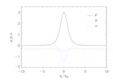
Figure 6: Components of the stress energy tensor (top panel) deduced from Eqs. (4) and (5) as functions of the conformal time $\eta/\eta_{0}$ for the scale factor (72). Shown are the values of the background energy density $\rho$ (full line), the pressure $p$ (dotted line) and their ratio $\omega$ (dashed line). In this figure as well as the following, the parameters have been given the particular values $\ell_{0}=1$ and $\eta_{0}=2$. The bottom panel displays the sound velocity $c_{{}_{\rm S}}^{2}$ as given by Eq. (73).

From the figures, one can already see that the bounce is rather unlikely to be well described by a sharp transition which would require a finite jump in both $\omega$ and $c_{{}_{\rm S}}^{2}$. One could however argue at this point that this is due to our approximation for the scale factor at the bounce: an even scale factor leads to an even equation of state and therefore to a transition which cannot be assumed sharp, even if the transition duration goes to zero.

Another, more important, reason to oppose the sharp transition treatment of the bounce lies in the following. In the neighborhood of the bounce we have

$$(\rho+p)(\eta=0)=\frac{2}{\ell_{0}^{2}}\biggl{(}1-\frac{1}{\eta_{0}^{2}}\biggr{)},$$ (74)

which can be easily interpreted. Restoring the usual units (with $c$ the velocity of light), the above equation can be rewritten as $\kappa(\rho+p)=2/\ell_{0}^{2}[{\cal K}-\ell_{0}^{2}/(c^{2}t_{0}^{2})]$, in which we interpret $\ell_{0}$ as the curvature scale [$\equiv a(\eta)/\sqrt{|{\cal K}|}$] at the bounce, and $t_{0}=\ell_{0}\eta_{0}/c$ is the physical time taken by light to go across the bounce. It makes sense that some exotic matter ($\rho+p<0$) is required if the growth of the universe is faster than light. Similarly, the sound velocity given by Eq. (8) reveals that if $\eta_{0}\leq 1$, there always is a point at which $c_{{}_{\rm S}}^{2}$ diverges. This is connected to the violation of the null energy condition ppnpn1 seen in Eq. (74). This has of course important consequences with respect to our wish to have a short duration bounce. In particular, it means that one cannot, in this framework, investigate the short bounce limit for which $\eta_{0}\to 0$. Therefore, we reach the conclusion that the time scale of the bounce cannot be made arbitrary short if we want to deal only with well-behaved quantities. This provides another argument against the sharp transition limit. We shall for now on restrict ourselves to the case $\eta_{0}>1$, which is consistent with our choice of setting ${\cal K}=1$ in order to avoid unnecessary exotic matter.

Let us now discuss the standard junction conditions. For the background, matching by brute force the pre- and post-impact phases (i.e., assuming that the bounce time scale is negligible) means $[{\cal H}]\neq 0$ since ${\cal H}$ has not the same sign before and after the bounce. On the other hand, the junction conditions applied to the background demand that $[{\cal H}]=0$. Therefore, it seems that it is already impossible to use the standard GR conditions at the background level, as pointed out in Ruth . This was also the reason why, in Ref. Ruth , a surface layer pressure term was introduced such as to allow for a jump in ${\cal H}$.

Accordingly, let us admit that we can study the perturbative level. It has been shown in Ref. MS that the well-known cosmological perturbation matching conditions for ${\cal K}=0$ also holds for ${\cal K}=1$. In this last case, the quantity $\zeta$ is not conserved, and it is better to work with another quantity $\zeta_{{}_{\mathrm{BST}}}$ defined by

$$\zeta_{{}_{\mathrm{BST}}} \equiv -\frac{2}{3}\frac{{\cal H}^{2}}{(1+\omega)({\cal H}^{2}+{\cal K})}\biggl{\{}{\cal H}^{-1}\Phi^{\prime}+\biggl{[}1-\frac{{\cal K}}{{\cal H}^{2}}+\frac{1}{3}\biggl{(}\frac{k}{{\cal H}}\biggr{)}^{2}\biggr{]}\Phi\biggr{\}}-\Phi$$ (75)

$$= -\frac{{\cal H}^{2}}{{\cal H}^{2}+{\cal K}}\zeta-\frac{k^{2}}{3\Gamma{\cal H}^{2}}\Phi-{\cal K}\biggl{(}\frac{1}{{\cal H}^{2}+{\cal K}}-\frac{1}{\Gamma{\cal H}^{2}}\biggr{)}\Phi.$$ (76)

The derivative with respect to conformal time of the previous quantity reads

$$\frac{1}{{\cal H}}\zeta_{{}_{\mathrm{BST}}}^{\prime}=-\frac{2}{3}\frac{{\cal H}^{2}}{(1+\omega)({\cal H}^{2}+{\cal K})}\biggl{[}\frac{1}{3}\biggl{(}\frac{k}{{\cal H}}\biggr{)}^{2}({\cal H}^{-1}\Phi^{\prime}+\Phi)\biggr{]}.$$ (77)

Therefore, we see that, even if ${\cal K}\neq 0$, $\zeta_{{}_{\mathrm{BST}}}$ is approximately constant on superhorizon scales and this property has been used in Refs. BF ; Hwang . With the exact toy model at our disposal, this can be explicitly tested.

We now turn to the study of the perturbed quantities. The effective potential $\theta^{\prime\prime}/\theta$, see Eq. (30), for the scalar perturbations is given in Fig. 7.

Figure 7: The parametric oscillator potential $\theta^{\prime\prime}/\theta$ [See Eqs. (30) and (31)] as functions of the conformal time with the same parameter as Fig. 6.

We assume that there is no entropy production and the equations governing the evolution of Bardeen potential are Eqs. (29) and (31). Two cases must be studied. In the short wavelength limit, for which $c_{{}_{\rm S}}^{2}(k^{2}-{\cal K})\gg\theta^{\prime\prime}/\theta$, $\zeta_{{}_{\mathrm{BST}}}$ is clearly not conserved. Therefore, the only case which remains to be studied is that of long wavelengths. The latter approximation can be applied if $c_{{}_{\rm S}}^{2}(k^{2}-{\cal K})\ll\theta^{\prime\prime}/\theta$, where $k=1,2,\cdots$. This is obviously true for $k=1$, i.e., a mode that cannot be confused with the background. This is less clear for higher $k$ modes, and depends on the parameter values. In the short bounce limit $\eta_{0}\to 1$ we are interested in, one has $c_{{}_{\rm S}}^{2}(\eta=0)\sim-(5/3)(\eta_{0}^{2}-1)^{-1}-1/3+{\cal O}(\eta_{0}^{2}-1)$ and $\theta^{\prime\prime}/\theta(\eta=0)\sim-(15/2)(\eta_{0}^{2}-1)^{-1}+3/2+{\cal O}(\eta_{0}^{2}-1)$, so that the ratio tends to the fixed value $9/2$. In this limit, the mode $k=2$ also marginally satisfies the long wavelength requirement. The approximation breaks down for $k\geq 3$. Since there exists at least one physically meaningfull mode for which the approximation is valid, we can proceed and use Eq. (33) for the relevant modes. In the case at hand, the integral can be performed exactly and the final result can be written as

$$\Phi(\eta,k) = B_{1}(k)\frac{3}{2\ell_{0}^{2}\eta_{0}}\frac{\eta}{\eta_{0}}\biggl{[}1+\frac{1}{2}\biggl{(}\frac{\eta}{\eta_{0}}\biggr{)}^{2}\biggr{]}^{-3}+B_{2}(k)\biggl{[}1+\frac{1}{2}\biggl{(}\frac{\eta}{\eta_{0}}\biggr{)}^{2}\biggr{]}^{-3}\biggl{[}1-\eta_{0}^{2}+\frac{1}{2}(4\eta_{0}^{2}+1)\biggl{(}\frac{\eta}{\eta_{0}}\biggr{)}^{2}$$ (78)

$$+\frac{1}{12}(6\eta_{0}^{2}+5)\biggl{(}\frac{\eta}{\eta_{0}}\biggr{)}^{4}+\frac{1}{40}(3+4\eta_{0}^{2})\biggl{(}\frac{\eta}{\eta_{0}}\biggr{)}^{6}+\frac{\eta_{0}^{2}}{112}\biggl{(}\frac{\eta}{\eta_{0}}\biggr{)}^{8}\biggr{]}.$$

As expected one branch is even and the other is odd. One also sees that if $\eta_{0}=1$ the minimum of the even branch is zero. This makes sense since in this case $\rho+p=0$, i.e., the de Sitter equation of state for which it is known that $\Phi=0$. The two branches are plotted in Fig. 8.

Figure 8: Odd (top) and even (bottom) modes of the Bardeen potential [see Eq. (78)] through the parabolic bounce as functions of the conformal time with the same parameter as Fig. 6.

We are now in the position where we can estimate $\zeta_{{}_{\mathrm{BST}}}$ for these long wavelength modes. Expanding Eq. (76) to leading order, one finds

$$\zeta_{{}_{\mathrm{BST}}}\simeq-\frac{{\cal H}^{2}}{{\cal H}^{2}+{\cal K}}B_{2}-{\cal K}\biggl{(}\frac{1}{{\cal H}^{2}+{\cal K}}-\frac{1}{\Gamma{\cal H}^{2}}\biggr{)}\Phi+{\cal O}(k^{2}).$$ (79)

In the above relation, only the $B_{2}$–mode of $\zeta$ appears in the first term since the $B_{1}$–term is of order $k^{2}B_{1}(k)$, see Eq. (46), whereas the corresponding term in the Bardeen potential is of order $B_{1}(k)$. Far from the bounce, when $\eta/\eta_{0}\gg 1$, the first term in Eq. (79) tends to zero, while the second goes to $-B_{2}/7$ on both sides, as can be explicitly checked in Figs. 9. Therefore, if we consider a long time interval $\Delta\eta/\eta_{0}\gg 1$, this quantity seems to be indeed constant. On the other hand, close to the bounce, over typical bounce time scales, i.e., $\Delta\eta/\eta_{0}\simeq 1$, one clearly sees in Figs. 9 that the quantity $\zeta_{{}_{\mathrm{BST}}}$ is not a constant. This is due to the fact that, during the bounce, the “growing” and “decaying” modes are of the same order of magnitude as shown in Fig. 9.

Figure 9: Two typical configurations for the supposedly conserved quantity $\zeta_{{}_{\mathrm{BST}}}$ as functions of the conformal time with the same parameter as on the previous figures. Top panel: $B_{1}=10$ and $B_{2}=1$. Bottom panel: $B_{1}=1$ and $B_{2}=10$.

To conclude this section, let us summarize what we have learned from the simple toy model used here: (i) we have seen that the standard GR junction conditions applied to the background are not consistent with a bounce since ${\cal H}$ has not the same sign before and after the bounce Ruth , (ii) we have shown that the equation of state does not jump at the bounce, (iii) we have found that a bounce cannot be made arbitrary short without violating the null energy condition ppnpn1 and finally (iv) we have noticed that the quantity $\zeta_{{}_{\mathrm{BST}}}$ is not constant on the typical bounce time scale (recall that beyond the bounce epoch, our model looses its meaning and should be matched to another era).

V A test scalar field in the ekpyrotic universe

Let us now turn to the last case for which one can explicitly calculate the various physically meaningful quantities during a regular bounce. We now assume that a bounce took place, and consider perturbations of a test scalar field in that background. In this case, we do not need to specify the origin of the scale factor. As in section IV, we question the conservation of what we know is conserved in sharp transitions. We can also regard the perturbations studied in this section as gravitational waves, provided then that ${\cal K}=0$ and that somehow the necessary modification of GR is negligible on the tensor part of the perturbations.

The equation of a test scalar field in a spatially FLRW spacetime with a scale factor given by the previous expression is

$$\mu^{\prime\prime}+\biggl{(}k^{2}-{{a^{\prime\prime}}\over a}\biggr{)}\mu\,=\,0\,.$$ (80)

As mentioned above, this is also the equation of motion of gravitational waves in GR if ${\cal K}=0$. The solution of this equation possesses two regimes determined by the relative contribution of the two terms $k^{2}$ and $a^{\prime\prime}/a$. The transition time $\eta_{\rm j}(k)$ is defined by $k^{2}=a^{\prime\prime}/a$. In the case of a parabolic scale factor, one has

$$\frac{a^{\prime\prime}}{a}=\frac{1}{\eta_{0}^{2}}\biggl{[}1+\frac{1}{2}\biggl{(}\displaystyle{\frac{\eta}{\eta_{0}}}\biggr{)}^{2}\biggr{]}^{-1}.$$ (81)

The maximum of the quantity $a^{\prime\prime}/a$ is $1/\eta_{0}^{2}$ and define the only characteristic scale of the problem, i.e., $k_{\rm max}=1/\eta_{0}$. Let us define the parameter $\epsilon$ by $\epsilon\equiv k/k_{\rm max}$, then one has

$$\eta_{\rm j}(k)=\pm\frac{\eta_{0}}{\epsilon}\sqrt{2(1-\epsilon^{2})}.$$ (82)

The next step is to solve the equation of motion. From the above considerations, we see that there are three different regions. In the first region where $\eta<-\eta_{\rm j}(k)$, we only consider positive frequency modes and we have

$$\mu_{\rm I}(\eta)=\frac{1}{\sqrt{2k}}\exp[-ik(\eta-\eta_{\rm i})]$$ (83)

where $\eta_{\rm i}$ is an arbitrary initial time. In the second region, where $-\eta_{\rm j}(k)<\eta<\eta_{\rm j}(k)$, the solution is given by

$$\mu_{\rm II}(\eta)=B_{1}a(\eta)+B_{2}a(\eta)\int_{0}^{\eta}\frac{{\rm d}\tau}{a^{2}({\tau})}.$$ (84)

The lower bound of the integral is a priori arbitrary. However, it is very convenient to take it equal to zero because in this case the second branch becomes odd whereas the first one (i.e., the scale factor) is even. Then, it is easy to show that

$$\int_{0}^{\eta}\frac{{\rm d}\tau}{a^{2}({\tau})}=\frac{\eta_{0}}{2\ell_{0}}\frac{1}{a(\eta)}\biggl{[}\frac{\eta}{\eta_{0}}+\frac{\sqrt{2}}{\ell_{0}}a(\eta)\tan^{-1}\biggl{(}\frac{\eta}{\sqrt{2}\eta_{0}}\biggr{)}\biggr{]}.$$ (85)

Finally, the solution in the third region where $\eta>\eta_{\rm j}(n)$ can be written as

$$\mu_{\rm III}(\eta)=\frac{C_{1}}{\sqrt{2k}}\exp(-ik\eta)+\frac{C_{2}}{\sqrt{2k}}\exp(+ik\eta).$$ (86)

Figure 10: The expectedly conserved quantity $\mu/a$ for a spectator scalar field (or gravitational wave production) in a bouncing universe, i.e., Eq. (85), with parameter fixed at $\ell_{0}=1$, $\eta_{0}=2.$, $B_{1}=1$ and $B_{2}=1$. It is clear on this figure that this quantity is not actually conserved through the bounce.

Fig. 10 shows the solution (85) as a function of the conformal time through the bounce. In the usual situation, the quantity $h=\mu/a$ is conserved because only the growing mode $a$ plays a role. In the present situation, it is clear that the usually conserved quantity is not actually conserved. The reason is that through the bounce the odd mode (which is the decaying mode in general) $a\int^{\rm\eta}{\rm d}\tau/a^{2}$ now plays a crucial role. Therefore if we match the bounce epoch to other eras before and after the impact, we see that the usual conservation cannot be used.

Since the conservation law cannot be utilized, one has to perform the calculation explicitly. Therefore, the goal is now to calculate the coefficients $C_{1}$ and $C_{2}$. Using the continuity of the mode function $\mu$ and of its derivative, we find

$$C_{1}(k) = \frac{\mbox{e}^{ik(2\eta_{\rm j}+\eta_{\rm i})}}{2ik}\biggl{\{}-[g^{\prime}+ikg](-\eta_{\rm j})[f^{\prime}-ikf](\eta_{\rm j})+[f^{\prime}+ikf](-\eta_{\rm j})[g^{\prime}-ikg](\eta_{\rm j})\biggr{\}},$$ (87)

$$C_{2}(k) = -\frac{\mbox{e}^{ik\eta_{\rm i}}}{2ik}\biggl{\{}-[g^{\prime}+ikg](-\eta_{\rm j})[f^{\prime}+ikf](\eta_{\rm j})+[f^{\prime}+ikf](-\eta_{\rm j})[g^{\prime}+ikg](\eta_{\rm j})\biggr{\}},$$ (88)

where we have used the short-hand notation $f\equiv a(\eta)$ and $g\equiv a(\eta)\int^{\eta}_{0}{\rm d}\tau/a^{2}(\tau)$. The final result is given by Eqs. (87), (88) where all the functions are explicitly known except the function $\eta_{\rm j}=\eta_{\rm j}(k)$. Expanding everything in terms of the small parameter $\epsilon$ one finds

$$C_{1}(k)=\frac{\pi}{4(k\eta_{0})^{3}}\mbox{e}^{2i\sqrt{2}}(4+i\sqrt{2})+{\cal O}(\epsilon^{-2}),\quad C_{2}(k)=-\frac{3i\pi}{2\sqrt{2}(k\eta_{0})^{3}}+{\cal O}(\epsilon^{-2}).$$ (89)

The spectrum is defined by the following expression

$$k^{3}P(k)=\frac{k^{3}}{2\pi^{2}}\biggl{|}\frac{\mu(+\eta_{\rm j})}{a(+\eta_{\rm j})}\biggr{|}^{2}.$$ (90)

Since the coefficients $C_{1}$ and $C_{2}$ are of the same order in $k$, as shown in Eqs. (89), the power spectrum $k^{3}P(k)$ will take the form of an overall power-law amplitude times an oscillatory function in $k$. If we parameterize the overall amplitude as $k^{n_{{}_{\rm S}}-1}$ for $k\ll k_{\rm max}$, one has $n_{{}_{\rm S}}=1$, i.e, a scale-invariant spectrum. In the other limit $k\gg k_{\rm max}$ where Eqs. (87), (88) cannot be used, the result is obvious since the $k^{2}$ term always dominates the effective potential $a^{\prime\prime}/a$ in Eq. (80): it is $n_{{}_{\rm S}}=3$. We also note that when $\eta_{0}\rightarrow 0$, the spectrum blows up and this provides another argument against a sharp bounce.

In order to test the dependence of the spectrum in the precise form of the bounce, it is interesting to calculate the spectrum for another scale factor. We choose

$$a(\eta)=\ell_{0}\sqrt{1+\biggl{(}\frac{\eta}{\eta_{0}}\biggr{)}^{2}}.$$ (91)

This case is treated in Ref. ppnpn2 . Let us notice that when $\eta$ is small (i.e., close to the bounce) the previous equation reduces to Eq. (72) as expected. Then straightforward calculations lead to, still for $k\ll k_{\rm max}$,

$$C_{1}(k)=\frac{i\pi}{2k\eta_{0}}+{\cal O}(\epsilon^{0}),\quad C_{2}(k)=-\frac{i\pi}{2k\eta_{0}}+{\cal O}(\epsilon^{0}).$$ (92)

In this case, since $C_{1}=-C_{2}$ at leading order, the oscillatory part of the power spectrum contributes in a non trivial way to the spectral index of the overall amplitude. We find $n_{{}_{\rm S}}=3$ which, by comparison with the spectrum obtained in Eq. (89), shows that this spectrum is very strongly dependent on the actual shape of the bounce. This was to be expected since the bounce has already been shown not to be a sharp transition.

The conclusion of this section is that the spectrum of gravitational waves (if we accept the trick that, in a bouncing universe, the spectrum of a free scalar field can be a good approximation of the actual gravitational waves spectrum) is in general more complicated than in the inflationary case. A first feature is that there exists a prefered scale the magnitude of which depends on the details of the model. A second property is that, generically, the power spectrum acquires superimposed oscillations due to the fact that, at last horizon entry, the two branches contribute equally. Therefore, the shape of the spectrum crucially depends on the details of the model.

VI Conclusions

The conclusions that can be drawn from this work is that it seems impossible to apply any known and well motivated criterion to pass through a bounce, whether regular or singular, in a model independent way as all quantities of interest explicitly depend on the details of the underlying model. The ekpyrotic model, although a potentially interesting alternative to the inflationary paradigm, does pass through such a bounce. Therefore, if one really wants to calculate the spectrum in the ekpyrotic universe then it seems necessary, first, to consider a situation where there is no divergence and, second, to provide us with the actual (maybe five-dimensional) equations of motion during the bounce, knowing that these equations cannot be those of GR.

- (1) M. B. Green, J. H. Schwarz and E. Witten, Superstring Theory, Cambridge University Press, Cambridge (1987); J. Polchinski, String Theory, Cambridge University Press, Cambridge (1998).
- (2) R. Gambini and J. Pullin, Loops, knots, gauge theories and quantum gravity (Cambridge University Press, Cambridge, UK, 1998) ; S. Carlip, Rep. Prog. Phys. 64, 885 (2001).
- (3) N. Arkani-Hamed, S. Dimopoulos and G. R. Dvali, Phys. Lett. B 429, 263 (1998); N. Arkani-Hamed, S. Dimopoulos and G. R. Dvali, Phys. Rev. D 59, 086004 (1999); I. Antoniadis, N. Arkani-Hamed, S. Dimopoulos and G. R. Dvali, Phys. Lett. B 436, 257 (1998);
- (4) L. Randall and R. Sundrum, Nucl. Phys. B 557, 79 (1999); Phys. Rev. Lett. 83, 3370 (1999); Phys. Rev. Lett. 83,4690 (1999).
- (5) A. H. Guth, Phys. Rev. D23, 347 (1981); A. D. Linde, Particle Physics and Inflationary Cosmology, (Harwood Academic, New-York, 1990).
- (6) A. Lukas, B. A. Ovrut and D. Waldram, Nucl. Phys. B 532, 43 (1998) ; Phys. Rev. D57, 7529 (1998); A. Lukas, B. A. Ovrut, K. S. Stelle and D. Waldram, Phys. Rev. D59, 086001 (1999).
- (7) P. Hořava and E. Witten, Nucl. Phys. B 460, 506 (1996) ; 475, 94 (1996).
- (8) J. Khoury, B. A. Ovrut, P. J. Steinhardt and N. Turok, Phys. Rev. D64, 123522 (2001).
- (9) J. Khoury, B. A. Ovrut, N. Seiberg, P. J. Steinhardt and N. Turok, hep-th/0108187.
- (10) J. Khoury, B. A. Ovrut, P. J. Steinhardt and N. Turok, hep-th/0109050.
- (11) R. Kallosh, L. Kofman and A. Linde, Phys. Rev. D64, 123523 (2001); R. Kallosh, L. Kofman, A. Linde and A. Tseytlin, Phys. Rev. D64, 123524 (2001).
- (12) G. Veneziano, Phys. Lett. B 265, 287 (1991); M. Gasperini and G. Veneziano, Astropart. Phys. 1, 317 (1993); See also J. E. Lidsey, D. Wands and E. J. Copeland, Phys. Rep. 337, 343 (2000); G. Veneziano, it in Les Houches, Session LXXI, The primordial Universe, P. Binétruy et al. Eds., (EDP Sciences & Springer, Paris, 2000).
- (13) E. B. Bogomolnyi, Sov. J. Phys. 24, 449 (1976); M. K. Prasad and C. M. Sommerfield, Phys. Rev. Lett. 35, 760 (1975).
- (14) D. H. Lyth, hep-ph/0106153; ibid. hep-ph/0110007; ibid. in preparation.
- (15) R. Brandenberger and F. Finelli, hep-th/0109004.
- (16) J. Hwang, astro-ph/0109045; J. Hwang and H. Noh, astro-ph/0112079.
- (17) J. M. Bardeen, Phys. Rev. D22, 1882 (1980).
- (18) V. F. Mukhanov, H. A. Feldman and R. H. Brandenberger, Phys. Rep. 215, 203 (1992).
- (19) J. Preskill, Phys. Rev. Lett. 43, 1365 (1979); E. P. S. Shellard and A. Vilenkin, Cosmic strings and other topological defects, Cambridge University Press (1994).
- (20) J. Martin and R. H. Brandenberger, Phys. Rev. D63, 123501 (2001); R. H. Brandenberger and J. Martin, Mod. Phys. Lett A 16, 999 (2001); R. H. Brandenberger, S. E. Jorás and J. Martin, hep-th/0112122.
- (21) J. Khoury, B. A. Ovrut, P. J. Steinhardt and N. Turok, hep-th/0105212.
- (22) P. Peter and N. Pinto-Neto, Phys. Rev. D(2001) in press gr-qc/0109038.
- (23) P. J. Steinhardt and N. Turok, hep-th/0111098.
- (24) L. F. Abbott and M. B. Wise, Nucl. Phys. B 244, 541 (1984).
- (25) J. Martin and D. J. Schwarz, Phys. Rev. D57, 3302 (1998).
- (26) I. S. Gradshteyn and I. M. Ryshik, Table of Integrals, Series and Products (Academic, New-York 1980).
- (27) L. Lewin Dilogarithms and associated functions (Macdonald, London, 1958).
- (28) J. Hwang and E. T. Vishniac, Astrophys. J. 382, 363 (1991); N. Deruelle and V. F. Mukhanov, Phys. Rev. D52, 5549 (1995).
- (29) R. Durrer, hep-th/0112026.
- (30) C. W. Misner, K. S. Thorne and J. A. Wheeler, Gravitation (W. H. Freeman and Company, New-York, 1973).
- (31) Ya. B. Zel’dovich and L. P. Pitaevsky, Commun. Math. Phys. 23, 185 (1971); S. W. Hawking and G. F. R. Ellis, The large scale structure of space-time, Cambridge University Press (1973); R. M. Wald., General Relativity, Chicago University Press (1984); L. A. Wu, H. J. Kimble, J. L. Hall and H. Wu, Phys. Rev. Let. 57, 2520 (1986). See also M. Visser, Phys. Lett. B 349, 443 (1995); A. Borde and A. Vilenkin, Phys. Rev. D56, 717 (1997); C. Barceló and M. Visser, Nucl. Phys. B 584, 415 (2000) for more recent discussions.
- (32) P. Peter and N. Pinto-Neto, in preparation.