General structure of the photon self-energy in non-commutative QED

Abstract

We study the behavior of the photon two point function, in non-commutative QED, in a general covariant gauge and in arbitrary space-time dimensions. We show, to all orders, that the photon self-energy is transverse. Using an appropriate extension of the dimensional regularization method, we evaluate the one-loop corrections, which show that the theory is renormalizable. We also prove, to all orders, that the poles of the photon propagator are gauge independent and briefly discuss some other related aspects.

I Introduction

Non-commutative theories have generated a lot of interest in recent years Gonzalez-Arroyo:1983ub ; Filk:1996dm ; Martin:1999aq ; Sheikh-Jabbari:1999iw ; Krajewski:1999ja ; Bigatti:1999iz ; Maldacena:1999mh ; Iso:2000ew ; Arcioni:1999hw ; Minwalla:1999px ; Aref'eva:1999sn ; Gross:2000ba ; Matusis:2000jf ; Hayakawa:1999zf ; girotti:2000gc ; Zanon:2000nq ; Das:2001kf ; Khoze:2000sy ; Liu:2000ad ; VanRaamsdonk:2001jd ; Armoni:2000xr ; Ruiz:2000hu ; Bichl:2001cq ; foot . These are theories defined on a manifold where the coordinates do not commute. As a result, in such theories, there is a natural second rank anti-symmetric tensor with the canonical dimension of inverse mass squared. Several interesting features develop in such theories. First of all, because of non-commutativity of coordinates, the natural product of functions, on such a space, is the star product of Grönewold and Moyal Groenewold:1946 ; Moyal:1949sk . One of the consequences of such a product is that, in a physical theory, the interaction terms develop a momentum dependent phase factor (in momentum space). However, the two point functions and, therefore, the propagators do not modify. Furthermore, explicit loop calculations show that the conventional ultraviolet terms in a commutative theory get distributed into two parts – one that is ultraviolet divergent while the other is ultraviolet finite. However, these ultraviolet finite terms become singular in the infrared limit and the amplitudes become non-analytic.

All these features are quite fascinating and puzzling, since they are somewhat similar to what happens in thermal field theories kapusta:book89 ; lebellac:book96 ; das:book97 . For example, we know that, at finite temperature, we have a new scale, the temperature, and an additional, natural Lorentz vector, $u^{\mu}$, which is the velocity of the heat bath. In a thermal field theory, however, the interaction vertices do not modify, rather the propagators do, because of (anti) periodic boundary conditions. In this sense, thermal field theories and non-commutative field theories seem complementary and a natural question of interest is whether there is any redefinition of variables that may map one to the other. It is also known that no new ultraviolet divergences develop at finite temperature. However, the infrared divergences do become more severe, once again similar to what happens in non-commutative theories, at least in one loop. Even more fascinating is the observation that, at finite temperature, amplitudes become non-analytic at the origin in the energy-momentum plane, which is reminiscent of the non-analyticity in non-commutative theories. In thermal field theories, the physical origin of the non-analyticity is well understood. Namely, in a thermal medium, new channels of reaction develop leading to new branch cuts, which is the reason for the non-analyticity. In the same spirit, it will be interesting to understand if there is a physical origin of the non-analyticity in non-commutative theories.

A lot is already known about thermal field theories and even though we do not yet know whether non-commutative theories and thermal theories can be mapped into each other, we may make use of some of the techniques that have been developed in connection with thermal field theories, to learn more about non-commutative field theories. It is with this goal that we take up a systematic study of the photon self-energy in non-commutative QED in a general covariant gauge in arbitrary dimensions. Since the contribution of the fermion loop to the photon self-energy has been studied in detail in the past, we concentrate only on the contributions coming from internal gauge and ghost loops. Our study leads to a number of interesting features that bring out similarities and differences between thermal field theories and non-commutative field theories. For example, we find that although non-commutative QED has a non-Abelian character because of the star product, the self-energy is transverse to all orders in a general covariant gauge in any dimension. This has to be contrasted with the self-energy of thermal QCD, which is, in general, not transverse. We verify this all orders result by explicitly calculating the self-energy at one loop. The calculations in a gauge theory are, of course, best carried out in dimensional regularization. However, most of the calculations in non-commutative theories, so far, have used the method due to Schwinger (the difficulty is mainly due to the exponential phase factor). Therefore, as a first step, we have generalized the formulae of dimensional regularization to non-commutative theories and this indeed simplifies the calculations quite a bit. The explicit calculation, at one loop, shows that the self-energy is gauge dependent, but does not develop any new kind of ultraviolet divergence, so that the theory is renormalizable. Furthermore, in the infrared limit, the imaginary part of the contributions to the self-energy, coming from these graphs, identically vanishes. This is, in fact, interesting in that the non-analyticity in the non-commutative QED does not seem to be connected with new imaginary parts in the amplitude. Away from the infrared, however, the self-energy does have imaginary parts which are necessary for unitarity. The gauge dependence of the self-energy raises the question of the behavior of the poles of the photon propagator in this theory and we prove to all orders, using the Nielsen identity das:book97 ; Nielsen:1975fs , that, in spite of the gauge dependence of the self-energy, the poles of the propagator are gauge independent.

The paper is organized as follows. In section II, we briefly review the structure of non-commutative QED. In section III, drawing from previous experience with thermal field theories, we show that the photon self-energy, in this theory, is transverse to all orders in a general covariant gauge in any dimension. In section IV, we generalize the formulae of dimensional regularization to non-commutative theories. One loop calculations, using dimensional regularization, are presented in section V, where we also talk about various aspects of the result. In section VI, we analyze the imaginary part of the photon self-energy and bring out some interesting features associated with it. In section VII, we prove, using the Nielsen identity, that the poles of the photon propagator are gauge independent to all orders. We present a short conclusion in section VIII and give details on the derivation of the Nielsen identity in the appendix.

II Non-commutative QED

Non-commutative QED differs from the conventional commutative QED in the following manner. First of all, the theory is defined on a manifold, where the coordinates do not commute. Rather, they satisfy

$$[x^{\mu},x^{\nu}]=i\theta^{\mu\nu}$$ (1)

where $\theta^{\mu\nu}=-\theta^{\nu\mu}$ has the canonical dimension of inverse mass squared. To avoid problems with unitarity, we will assume that only the space-space components of $\theta^{\mu\nu}$ are nonzero, namely, that the time coordinate commutes with all the coordinates. An immediate consequence of the non-commutativity of coordinates is that products of functions on this manifold are naturally defined by the Grönewold-Moyal star product

$$f(x)\star g(x)=\left[e^{{i\over 2}\theta^{\mu\nu}\partial_{\mu}^{(\zeta)}\partial_{\nu}^{(\eta)}}f(x+\zeta)g(x+\eta)\right]_{\zeta=0=\eta}$$ (2)

The star product also naturally introduces a Moyal bracket of two bosonic functions as

$$[f,g]_{\rm MB}=f\star g-g\star f$$ (3)

With these, we can define the action for non-commutative QED as

$$S_{\rm inv}=\int d^{n}x\,{\cal L}_{\rm inv}=\int d^{n}x\,\left(-{1\over 4}F_{\mu\nu}\star F^{\mu\nu}+\bar{\psi}\star(iD\!\!\!\!/-m)\psi\right)$$ (4)

where $n$ is the number of space-time dimensions and

$$D_{\mu}\psi = \partial_{\mu}\psi-ieA_{\mu}\star\psi$$

$$F_{\mu\nu} = \partial_{\mu}A_{\nu}-\partial_{\nu}A_{\mu}-ie[A_{\mu},A_{\nu}]_{\rm MB}$$ (5)

This action can be easily verified to be invariant under the gauge transformations

$$\psi(x) \rightarrow \psi^{\prime}(x)=U(x)\star\psi(x)$$

$$A_{\mu}(x) \rightarrow A_{\mu}^{\prime}(x)=U(x)\star A_{\mu}(x)\star U^{-1}(x)+{i\over e}U(x)\star\partial_{\mu}U^{-1}(x)$$ (6)

Infinitesimally, the transformations take the form

$$\delta\psi(x) = i\epsilon(x)\star\psi(x)$$

$$\delta A_{\mu} = {1\over e}\,D_{\mu}\epsilon(x)={1\over e}\left(\partial_{\mu}\epsilon-ie\left[A_{\mu},\epsilon\right]_{\rm MB}\right)$$ (7)

where $\epsilon(x)$ is the parameter of infinitesimal transformations. We can, of course, add to this action a gauge fixing and a ghost action. For covariant gauge fixing, they will have the form

$$S_{\rm gf}+S_{\rm ghost}=\int d^{n}x\,\left(-{1\over 2\xi}(\partial_{\mu}A^{\mu})\star(\partial_{\nu}A^{\nu})+\partial^{\mu}\overline{c}\star(\partial_{\mu}c-ie[A_{\mu},c]_{\rm MB})\right)$$ (8)

where $\xi$ is the gauge fixing parameter. We note, therefore, that we can write the complete action for non-commutative QED in a general covariant gauge as

$$S=S_{\rm inv}+S_{\rm gf}+S_{\rm ghost}$$ (9)

Thus, we see that because of the star product, the action in (9), for non-commutative QED, has a non-Abelian structure through the Moyal bracket. The star product has some interesting consequences. In particular, under an integral, the star product of two functions is the same as an ordinary product (namely, the difference between the two integrands is a total divergence that integrates to zero for functions with appropriate asymptotic fall off). Similarly, the star product of any number of functions, under an integral, satisfies cyclicity. As a result of these, it follows that the two point functions and the propagators of a non-commutative field theory are the same as their commutative counterparts. However, the interaction vertices have an exponential dependence on $\theta^{\mu\nu}$ as well as the momenta carried by the fields. Thus, for example, for the action in (9), the Feynman rules for the theory are as follows. First, the propagators of the theory are

$$:\;\;\; \;\;\;\displaystyle{{i\over p\!\!\!/-m+i\epsilon}=iS(p)}$$

$$:\;\;\; \;\;\;-\displaystyle{{i\over(p^{2}+i\epsilon)}\left(\eta_{\mu\nu}-(1-\xi){p_{\mu}p_{\nu}\over p^{2}}\right)=iD_{\mu\nu}(p)}$$

$$:\;\;\; \;\;\;\displaystyle{{i\over p^{2}+i\epsilon}=iD(p)}$$ (10)

These are the same as in the commutative theory. Introducing the notation,

$$p\times q=\theta^{\mu\nu}p_{\mu}q_{\nu}$$ (11)

the vertices, on the other hand, have the following forms (with the momentum conserving delta functions omitted)

$$\begin{array}[]{c}\includegraphics*{f14_gluon_fermion.eps}\end{array} :\;\;\; \;\;\;ie\gamma^{\mu}e^{{i\over 2}p_{i}\times p_{f}}$$ (13)

$$\begin{array}[]{c}\includegraphics*{f15_gluon_vert.eps}\end{array} :\;\;\; \;\;\;-2i\,e\sin{p_{1}\times p_{2}\over 2}\left[(p_{1}-p_{2})^{\lambda}\eta^{\mu\nu}+(p_{2}-p_{3})^{\mu}\eta^{\nu\lambda}+(p_{3}-p_{1})^{\nu}\eta^{\lambda\mu}\right]$$ (15)

$$\begin{array}[]{c}\includegraphics*{f16_quart.eps}\end{array} :\;\;\; \;\;\;-4\,e^{2}\left[(\eta^{\mu\lambda}\eta^{\nu\rho}-\eta^{\mu\rho}\eta^{\nu\lambda})\sin{p_{1}\times p_{2}\over 2}\sin{p_{3}\times p_{4}\over 2}\right.$$

$$\qquad\quad+(\eta^{\mu\rho}\eta^{\nu\lambda}-\eta^{\mu\nu}\eta^{\lambda\rho})\sin{p_{3}\times p_{1}\over 2}\sin{p_{2}\times p_{4}\over 2}$$

$$\qquad\quad\left.+(\eta^{\mu\nu}\eta^{\lambda\rho}-\eta^{\mu\lambda}\eta^{\nu\rho})\sin{p_{1}\times p_{4}\over 2}\sin{p_{2}\times p_{3}\over 2}\right]$$

$$\begin{array}[]{c}\includegraphics*{f17_gluon_ghost.eps}\end{array} :\;\;\; \;\;\;2iep_{f}^{\mu}\sin{p_{i}\times p_{f}\over 2}$$ (19)

In this paper, we will study, systematically, the photon self-energy, at one loop, in a general covariant gauge in an arbitrary dimension. Since the fermion contribution to this is the same as in a commutative theory (namely, the diagram is “ planar”), and has been studied in the literature, we will concentrate only on the other graphs, which do not occur in commutative QED. The star product, of course, introduces a non-Abelian structure in this theory. But more than that, in such theories, we have an independent Lorentz structure which can, in principle, introduce a behavior parallel to that at finite temperature. For example, in the self-energy, there is one independent external momentum so that we can think of $\bar{u}^{\mu}=\theta^{\mu\nu}p_{\nu}$ as being analogous to the component of the velocity of the heat bath perpendicular to momentum at finite temperature. A lot is known about the self-energy of commutative Yang-Mills theory at finite temperature and our goal is to exploit the known features of such studies to understand the behavior of the self-energy in non-commutative QED in a general covariant gauge in any dimension. Even though our actual calculations are at one loop, in the process, we will find some interesting all orders results for the self-energy as well as the propagator in non-commutative QED.

III Transversality of the polarization tensor

It is well known in commutative QCD that, at finite temperature, the self-energy is not transverse in a general covariant gauge kobes:1989up ; brandt:1997se (It is transverse at one loop, only in the Feynman gauge). In spite of the apparent similarity of non-commutative theories with thermal field theories, we will show in the following that the photon self-energy in non-commutative QED is transverse to all orders in any covariant gauge and in any dimension, which is the behavior of the gauge self-energy in commutative QCD at zero temperature.

To show this, let us introduce some techniques from finite temperature field theory Weldon:1996kb . Consider a theory with a natural vector $u^{\mu}$ (for example, the velocity of the heat bath at finite temperature). Then, given a momentum vector $p^{\mu}$, let us define the component of $u^{\mu}$ orthogonal to $p^{\mu}$ as

$$\bar{u}^{\mu}=\left(u^{\mu}-{(u\cdot p)\over p^{2}}\,p^{\mu}\right),\qquad p_{\mu}\bar{u}^{\mu}=0$$ (20)

In such a theory, the self-energy for the gauge field will have the most general, all orders decomposition given by

$$\Pi^{\mu\nu}=A\,\left(\eta^{\mu\nu}-{p^{\mu}p^{\nu}\over p^{2}}\right)+B\,{\bar{u}^{\mu}\bar{u}^{\nu}\over\bar{u}^{2}}+C\,{p^{\mu}\bar{u}^{\nu}+p^{\nu}\bar{u}^{\mu}\over\bar{u}^{2}}+D\,{p^{\mu}p^{\nu}\over p^{2}}$$ (21)

It follows from this that

$$p_{\mu}\Pi^{\mu\nu}={Cp^{2}\over\bar{u}^{2}}\,\bar{u}^{\nu}+Dp^{\nu}\neq 0$$ (22)

unless $C=0=D$.

Adding the tree level two point function, we can write the complete two point function to all orders as

$$\Gamma^{\mu\nu} = \widehat{\Gamma}^{\mu\nu}+{p^{\mu}p^{\nu}\over\xi}$$ (23)

$$= \left[(p^{2}+A)\,\left(\eta^{\mu\nu}-{p^{\mu}p^{\nu}\over p^{2}}\right)+B\,{\bar{u}^{\mu}\bar{u}^{\nu}\over\bar{u}^{2}}+C\,{p^{\mu}\bar{u}^{\nu}+p^{\nu}\bar{u}^{\mu}\over\bar{u}^{2}}+D\,{p^{\mu}p^{\nu}\over p^{2}}\right]+{p^{\mu}p^{\nu}\over\xi}$$

The complete propagator is defined to be

$$\Gamma^{\mu\nu}D_{\nu\lambda}=-\delta^{\mu}_{\lambda}$$ (24)

and satisfies, in consequence of the Slavnov-Taylor identity Taylor:ff ,

$$p^{\mu}p^{\nu}D_{\mu\nu}=-\xi$$ (25)

Let us now define

$$G_{\mu}=p^{\nu}D_{\mu\nu},\qquad p^{\mu}G_{\mu}=-\xi$$ (26)

Then, it follows, in a simple manner, that

$$\widehat{\Gamma}^{\mu\nu}G_{\nu}=\left(\Gamma^{\mu\nu}-{p^{\mu}p^{\nu}\over\xi}\right)p^{\rho}D_{\nu\rho}=-p^{\mu}+p^{\mu}=0$$ (27)

This shows that $\widehat{\Gamma}^{\mu\nu}$ has a zero mode, which can be explicitly constructed to be

$$G^{0}_{\mu}=-{\xi\over p^{2}}\left(p_{\mu}-{D\over C}\,\bar{u}_{\mu}\right)$$ (28)

with

$$D={p^{2}C^{2}\over\bar{u}^{2}(p^{2}+A+B)}$$ (29)

Thus far, our analysis has been quite general. Let us next turn to non-commutative QED. In this case, we can identify

$$\bar{u}^{\mu}=\theta^{\mu\nu}p_{\nu}$$ (30)

Furthermore, from the Feynman rules, let us note that the self-energy diagrams (involving internal photon and ghost lines) are invariant under

$$\theta^{\mu\nu}\rightarrow-\theta^{\mu\nu}$$

Therefore, the self-energy must be an even function of $\bar{u}^{\mu}$. (We note here that this property holds even with fermion interactions and is a consequence of charge conjugation invariance of the two point function Sheikh-Jabbari:2000vi .) It follows, then, that the coefficient, $C$, in (21) must be odd in $\bar{u}^{\mu}$. Since it is a scalar function, the most general form it can have is

$$C=(\bar{u}\cdot p)\,E=0$$ (31)

where $E$ denotes a scalar function, even in $\bar{u}^{\mu}$, and we have used the fact that $\bar{u}^{\mu}$ is orthogonal to $p^{\mu}$. Since $C=0$, it follows from (29) that $D=0$.

Therefore, to all orders, we determine that the most general form for the self-energy in non-commutative QED, in a general covariant gauge in any dimension, can be written as

$$\Pi^{\mu\nu}=A\,\left(\eta^{\mu\nu}-{p^{\mu}p^{\nu}\over p^{2}}\right)+B\,{\bar{u}^{\mu}\bar{u}^{\nu}\over\bar{u}^{2}}$$ (32)

which is manifestly transverse. (Note that, in this case, the zero mode in (28) simply reduces to $-\xi p_{\mu}/p^{2}$.) The coefficients $A$ and $B$, of course, will be dependent on the gauge fixing parameter, unlike in commutative QED, and we would like to evaluate these functions at one loop.

IV Dimensional regularization in non-commutative field theory

The calculations in non-commutative field theory have so far been mostly carried out using the methods of Schwinger. However, from studies in commutative gauge field theories, we know that dimensional regularization 'thooft:1972fi is extremely simple and powerful which, while maintaining gauge invariance, allows the proof of many results in a natural manner. Therefore, it is quite useful to try to extend the method of dimensional regularization to non-commutative theories Armoni:2000xr ; Ruiz:2000hu . In what follows, we will derive the dimensional regularization formulae, relevant to non-commutative theories in two different ways, both leading to the same results.

In non-commutative theories (for example, in non-commutative QED, see (19)), the interactions involve a momentum dependent phase factor. Therefore, a generic loop integral, that arises in such theories, has the form

$$I=\int{d^{n}k\over(2\pi)^{n}}\,{e^{i\bar{\theta}\cdot k}\over(k^{2}-M^{2})^{\alpha}}$$ (33)

where we have defined

$$\bar{\theta}^{\mu}=\theta^{\mu\nu}f_{\mu}(p_{1},\cdots,p_{n})$$ (34)

with $f_{\mu}$ representing a function of the external momenta, $p_{1},\cdots,p_{n}$, and $M^{2}$ represents the term that arises from combining denominators using the Feynman parameters and shifting. $M^{2}$, in general, depends on the external momenta, masses of the theory as well as the Feynman parameters. For simplicity, we have ignored writing the integration over the Feynman parameters that needs to be carried out. To evaluate this integral, we first rotate to Euclidean space, so that we have (note that with our choice of $\theta^{\mu\nu}$ having only space indices, the exponent does not change sign upon rotation to Euclidean space)

$$I=i(-1)^{\alpha}\int{d^{n}k\over(2\pi)^{n}}\,{e^{i\bar{\theta}\cdot k}\over(k^{2}+M^{2})^{\alpha}}$$ (35)

It is the momentum dependent exponential that seems formidable. However, it turns out that it is not hard to evaluate integrals of this kind and let us present two different, but equivalent ways that lead to the same result. First of all, let us decompose the vector $k_{\mu}$ to longitudinal and transverse components with respect to $\bar{\theta}_{\mu}$. Let us introduce the decomposition,

$$k_{\|\,\mu}={\bar{\theta}\cdot k\over\bar{\theta}^{2}}\,\bar{\theta}_{\mu},\qquad k_{\bot\,\mu}=k_{\mu}-k_{\|\,\mu}$$ (36)

so that

$$\bar{\theta}\cdot k_{\|}=\bar{\theta}\cdot k,\qquad\bar{\theta}\cdot k_{\bot}=0$$ (37)

In terms of these components, then, we can write

$$I = {i(-1)^{\alpha}\over(2\pi)^{n}}\int dk_{\|}\,e^{i\bar{\theta}\cdot k_{\|}}\int d^{n-1}k_{\bot}\,{1\over(k_{\bot}^{2}+k_{\|}^{2}+M^{2})^{\alpha}}$$ (38)

$$= {i(-1)^{\alpha}\over(2\pi)^{n}}\int_{-\infty}^{\infty}dk_{\|}\,{\pi^{n-1\over 2}\Gamma(\alpha-{n-1\over 2})\over\Gamma(\alpha)}{e^{i\bar{\theta}\cdot k_{\|}}\over(k_{\|}^{2}+M^{2})^{\alpha-{n-1\over 2}}}$$

$$= {2i(-1)^{\alpha}\over(2\pi)^{n}}\,{\pi^{n-1\over 2}\Gamma(\alpha-{n-1\over 2})\over\Gamma(\alpha)}\int_{0}^{\infty}dk_{\|}\,{\cos\bar{\theta}\cdot k_{\|}\over(k_{\|}^{2}+M^{2})^{\alpha-{n-1\over 2}}}$$

Recalling that $k_{\|\,\mu}$ is parallel to $\bar{\theta}_{\mu}$, we note that $\cos\bar{\theta}\cdot k_{\|}=\cos|\bar{\theta}|k_{\|}$ where $|\bar{\theta}|=(-\bar{\theta}_{\mu}\bar{\theta}_{\mu})^{1\over 2}$ and $k_{\|}=(k_{\|\,\mu}k_{\|\,\mu})^{1\over 2}$. Therefore, defining a new variable $x=|\bar{\theta}|k_{\|}$, we can write the integral as

$$I = {2i(-1)^{\alpha}\over(2\pi)^{n}}\,{\pi^{n-1\over 2}\Gamma(\alpha-{n-1\over 2})\over\Gamma(\alpha)}\,|\bar{\theta}|^{2\alpha-n}\int_{0}^{\infty}dx\,{\cos x\over(x^{2}+(|\bar{\theta}|M)^{2})^{\alpha-{n-1\over 2}}}$$ (39)

$$= 2i(-1)^{\alpha}{\pi^{n-1\over 2}\over(2\pi)^{n}}\,{\Gamma(\alpha-{n-1\over 2})\over\Gamma(\alpha)}\,|\bar{\theta}|^{2\alpha-n}\times{(2|\bar{\theta}|M)^{{n\over 2}-\alpha}\over\sqrt{\pi}}\,\cos\pi({n\over 2}-\alpha)\Gamma({n+1\over 2}-\alpha)K_{\alpha-{n\over 2}}(|\bar{\theta}|M)$$

$$= i(-1)^{\alpha}{\pi^{n\over 2}\over(2\pi)^{n}}\,{1\over\Gamma(\alpha)}\,{1\over(M^{2})^{\alpha-{n\over 2}}}\,2\left({|\bar{\theta}|M\over 2}\right)^{\alpha-{n\over 2}}\,K_{\alpha-{n\over 2}}(|\bar{\theta}|M)$$

Here $K_{\alpha}$ denotes the Bessel function and, in the intermediate steps, we have used some identities involving the gamma functions gradshteyn . It is worth pointing out here that the identification of the last integral with the Bessel function is strictly valid when $n<2\alpha+1$, where it is straightforward to show, with the help of standard tables that

$$\lim_{z\rightarrow 0}\,z^{\nu}K_{\nu}(z)\longrightarrow 2^{\nu-1}\Gamma(\nu)$$ (40)

so that we have

$$\lim_{\bar{\theta}\rightarrow 0}\,I\rightarrow i(-1)^{\alpha}{\pi^{n\over 2}\over(2\pi)^{n}}\,{\Gamma(\alpha-{n\over 2})\over\Gamma(\alpha)}\,{1\over(M^{2})^{\alpha-{n\over 2}}}$$ (41)

However, as in dimensional regularization in commutative theories, we analytically continue this result to other dimensions.

Let us next give an alternate derivation of the dimensional regularization formula for our basic integral. We note that

$$I = i(-1)^{\alpha}\int{d^{n}k\over(2\pi)^{n}}\,{e^{i\bar{\theta}\cdot k}\over(k^{2}+M^{2})^{\alpha}}$$ (42)

$$= {i(-1)^{\alpha}\over\Gamma(\alpha)}\,\left(-{\partial\over\partial M^{2}}\right)^{\alpha-1}\int{d^{n}k\over(2\pi)^{n}}\,{e^{i\bar{\theta}\cdot k}\over k^{2}+M^{2}}$$

$$= {i(-1)^{\alpha}\over\Gamma(\alpha)}\left(-{\partial\over\partial M^{2}}\right)^{\alpha-1}\int{d^{n}k\over(2\pi)^{n}}\int_{0}^{\infty}d\lambda\,e^{-\lambda(k^{2}+M^{2})+i\bar{\theta}\cdot k}$$

$$= {i(-1)^{\alpha}\pi^{n\over 2}\over(2\pi)^{n}}{1\over\Gamma(\alpha)}\int_{0}^{\infty}d\lambda\,\lambda^{\alpha-1-{n\over 2}}\,e^{-\lambda M^{2}-{|\bar{\theta}|^{2}\over 4\lambda}}$$

$$= i(-1)^{\alpha}{\pi^{n\over 2}\over(2\pi)^{n}}\,{1\over\Gamma(\alpha)}\,{1\over(M^{2})^{\alpha-{n\over 2}}}\,2\left({|\bar{\theta}|M\over 2}\right)^{\alpha-{n\over 2}}\,K_{\alpha-{n\over 2}}(|\bar{\theta}|M)$$

which is exactly the same formula as derived earlier in (39).

This, therefore, generalizes dimensional regularization to non-commutative theories and evaluates the basic integral that arises in a non-commutative field theory. In the study of self-energy in gauge theories, however, we need integrals involving additional tensor structures, which can be evaluated in the following simple manner. First, let us note that, if we are interested in the self-energy, there is only one independent external momentum and, therefore,

$$\bar{\theta}_{\mu}=\theta_{\mu\nu}p_{\nu}$$ (43)

where $p_{\mu}$ is the external momentum. Second, in this case, $M^{2}=x(1-x)p^{2}$, where $x$ is the Feynman parameter that arises in combining two denominators. Now, if we introduce an auxiliary vector $z_{\mu}$, then, we obtain, following our earlier derivation in (39), that

$$I(z)=i(-1)^{\alpha}\int{d^{n}k\over(2\pi)^{n}}\,{e^{i(\bar{\theta}+z)\cdot k}\over(k^{2}+M^{2})^{\alpha}}=i(-1)^{\alpha}{\pi^{n\over 2}\over(2\pi)^{n}}\,{1\over\Gamma(\alpha)(M^{2})^{\alpha-{n\over 2}}}\,2\left({|\bar{\theta}+z|M\over 2}\right)^{\alpha-{n\over 2}}\,K_{\alpha-{n\over 2}}(|\bar{\theta}+z|M)$$ (44)

For small values of $z^{\mu}$, expanding in a Taylor series and using identities involving the Bessel functions, this result would generate the integrals involving all other tensor structures.

For completeness, we list below the Euclidean forms of the integrals that we will need in the subsequent sections.

$$\int{d^{n}k\over(2\pi)^{n}}\,{e^{i\bar{\theta}\cdot k}\over(k^{2}+M^{2})^{\alpha}} = {\pi^{n\over 2}\over(2\pi)^{n}}\,{1\over\Gamma(\alpha)}\,{1\over(M^{2})^{\alpha-{n\over 2}}}\,2\left({|\bar{\theta}|M\over 2}\right)^{\alpha-{n\over 2}}\,K_{\alpha-{n\over 2}}(|\bar{\theta}|M)$$

$$\int{d^{n}k\over(2\pi)^{n}}\,{e^{i\bar{\theta}\cdot k}\,(\bar{\theta}\cdot k)^{2}\over(k^{2}+M^{2})^{\alpha}} = {\pi^{n\over 2}\over(2\pi)^{n}}\,{1\over\Gamma(\alpha)}\,{|\bar{\theta}|^{2}\over(M^{2})^{\alpha-1-{n\over 2}}}\left[(2\alpha-1-n)\left({|\bar{\theta}|M\over 2}\right)^{\alpha-1-{n\over 2}}K_{\alpha-1-{n\over 2}}(|\bar{\theta}|M)\right.$$

$$\qquad\qquad\qquad\qquad\left.-2\left({|\bar{\theta}|M\over 2}\right)^{\alpha-{n\over 2}}K_{\alpha-{n\over 2}}(|\bar{\theta}|M)\right]$$

$$\int{d^{n}k\over(2\pi)^{n}}\,{e^{i\bar{\theta}\cdot k}\,k_{\mu}k_{\nu}\over(k^{2}+M^{2})^{\alpha}} = A_{\alpha}\delta_{\mu\nu}+B_{\alpha}{\bar{\theta}_{\mu}\bar{\theta}_{\nu}\over\bar{\theta}^{2}}$$ (45)

where

$$A_{\alpha} = {\pi^{n\over 2}\over(2\pi)^{n}}\,{1\over\Gamma(\alpha)}\,{1\over(M^{2})^{\alpha-1-{n\over 2}}}\,\left({|\bar{\theta}|M\over 2}\right)^{\alpha-1-{n\over 2}}K_{\alpha-1-{n\over 2}}(|\bar{\theta}|M)$$

$$B_{\alpha} = {\pi^{n\over 2}\over(2\pi)^{n}}\,{1\over\Gamma(\alpha)}\,{1\over(M^{2})^{\alpha-1-{n\over 2}}}\,\left[(2\alpha-2-n)\left({|\bar{\theta}|M\over 2}\right)^{\alpha-1-{n\over 2}}K_{\alpha-1-{n\over 2}}(|\bar{\theta}|M)-2\left({|\bar{\theta}|M\over 2}\right)^{\alpha-{n\over 2}}K_{\alpha-{n\over 2}}(|\bar{\theta}|M)\right]$$ (46)

V Explicit one loop calculation

In this section, we will explicitly evaluate the self-energy at one loop, using dimensional regularization. However, even before doing the calculation, let us verify explicitly that the self-energy is indeed transverse at one loop, as a check on our general result of section III.

There are three graphs for the self-energy, at one loop, that we are interested in, namely, the one with the internal ghost loop, the tadpole involving the four photon vertex and the one involving an internal gauge loop (see figures 1a, 1b and 1c).

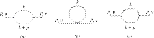
Figure 1: One-loop diagrams which contribute to the photon-self energy. Wavy and dashed lines denote respectively photons and ghosts. The external momenta on the left side is inward.

Each of these three graphs has the form (see(10,19))

$$\Pi_{\mu\nu}^{(I)}={e^{2}C^{(I)}\over 2}\,\int{d^{n}k\over(2\pi)^{n}}\,{(1-\cos p\times k)\over k^{2}(k+p)^{2}}\,N_{\mu\nu}^{(I)};\;\;\;\;\;\;\;\;\;\;\;I=a,b,c$$ (47)

where

$$C^{\rm(ghost)} = 1,\quad C^{\rm(tadpole)}={1\over 4},\quad C^{\rm(gauge)}={1\over 2}$$

$$N_{\mu\nu}^{\rm(ghost)} = 2(k+p)_{\mu}k_{\nu}$$

$$N_{\mu\nu}^{\rm(tadpole)} = -8(k+p)^{2}\left[(1-n)\eta_{\mu\nu}+(1-\xi)\,\left(\eta_{\mu\nu}-{k_{\mu}k_{\nu}\over k^{2}}\right)\right]$$

$$N_{\mu\nu}^{\rm(gauge)} = R_{\mu\nu}+(1-\xi)S_{\mu\nu}+(1-\xi)^{2}T_{\mu\nu}$$ (48)

where

$$R_{\mu\nu} = 2\left[(3+n)p_{\mu}p_{\nu}+(6-4n)k_{\mu}k_{\nu}-2\eta_{\mu\nu}(k^{2}+2p^{2})\right]$$

$$S_{\mu\nu} = 2\left[{(k^{2}+2p\cdot k)^{2}\over k^{2}}\,\eta_{\mu\nu}-{k^{2}+2p\cdot k-p^{2}\over k^{2}}\,k_{\mu}k_{\nu}+p_{\mu}p_{\nu}-{k^{2}+3p\cdot k\over k^{2}}\,(k_{\mu}p_{\nu}+k_{\nu}p_{\mu})+(k\rightarrow k+p,p\rightarrow-p)\right]$$

$$T_{\mu\nu} = -2\,{(p^{2}k_{\mu}-p\cdot k\,p_{\mu})(p^{2}k_{\nu}-p\cdot k\,p_{\nu})\over k^{2}(k+p)^{2}}$$ (49)

Thus, adding the three terms, we see that the self-energy has a natural expansion in powers of $(1-\xi)$ ($\xi=1$ corresponds to the Feynman gauge). The terms proportional to $(1-\xi)^{2}$ come only from the graph with the gauge loop and its structure, as can be seen from (49), is manifestly transverse. There are two terms proportional to $(1-\xi)$, coming from the tadpole as well as the gauge loop diagrams. If we add them, combine the denominators using Feynman parameters and shift the integration variable, we obtain

$$\Pi_{\mu\nu}^{(1-\xi)} = {4e^{2}(1-\xi)\over(2\pi)^{n}}\int_{0}^{1}dx(1-x)\int d^{n}k\,{(1-\cos p\times k)\over(k^{2}+x(1-x)p^{2})^{3}}$$ (50)

$$\quad\times\left[\left((1+2x)k^{2}p^{2}-4(1-x)(p\cdot k)^{2}-x^{2}(3-2x)(p^{2})^{2}\right)\eta_{\mu\nu}-2p^{2}k_{\mu}k_{\nu}\right.$$

$$\qquad\left.-\left((1+2x)k^{2}-x^{2}(3-2x)p^{2}\right)p_{\mu}p_{\nu}+(3-2x)p\cdot k(k_{\mu}p_{\nu}+k_{\nu}p_{\mu})\right]$$

Contracting with $p_{\mu}$, it can be seen that this vanishes upon symmetric integration. Therefore, the terms linear in $(1-\xi)$ are explicitly transverse as well. In a similar manner, it can also be checked that the terms independent of $(1-\xi)$ are transverse. Alternatively, let us note that the terms independent of $(1-\xi)$ would correspond to the self-energy in the Feynman gauge ($\xi=1$), which have been explicitly checked earlier to be transverse at one loop.

Thus, we see from the structure of the graphs that they are manifestly transverse at one loop, consistent with our all orders result. Thus, let us parameterize the self-energy as in (32) (with the identification $\bar{u}^{\mu}\equiv\bar{\theta}^{\mu}=\theta^{\mu\nu}p_{\nu}$) and write

$$\Pi_{\mu\nu}=A\,\left(\eta_{\mu\nu}-{p_{\mu}p_{\nu}\over p^{2}}\right)+B\,{\bar{\theta}_{\mu}\bar{\theta}_{\nu}\over\bar{\theta}^{2}}$$ (51)

It follows from this that

$$A = {1\over(n-2)}\,\left(\eta^{\mu\nu}\Pi_{\mu\nu}-{\bar{\theta}^{\mu}\bar{\theta}^{\nu}\over\bar{\theta}^{2}}\Pi_{\mu\nu}\right)$$

$$B = {1\over(n-2)}\,\left(-\eta^{\mu\nu}\Pi_{\mu\nu}+(n-1){\bar{\theta}^{\mu}\bar{\theta}^{\nu}\over\bar{\theta}^{2}}\,\Pi_{\mu\nu}\right)$$ (52)

In spite of the appearance of $(n-2)$ factors in the denominator, we will see that these quantities are well behaved at $n=2$ (namely, two dimensions).

Let us further expand each of these coefficients in powers of $(1-\xi)$,

$$A = A_{0}+(1-\xi)A_{1}+(1-\xi)^{2}A_{2}$$

$$B = B_{0}+(1-\xi)B_{1}+(1-\xi)^{2}B_{2}$$ (53)

where we have used the fact that the self-energy diagrams are at most quadratic in $(1-\xi)$. The subscripts here correspond to the power of $(1-\xi)$ and the lowest order terms simply correspond to the coefficients in the Feynman gauge. We can combine denominators and integrate over the internal momenta using formulae (45) for the terms depending on $\cos p\times k$ and use the conventional formulae of dimensional regularization for the term independent of $\theta^{\mu\nu}$. As we have mentioned earlier, the usual results of dimensional regularization can be obtained through the simple substitution

$$z^{\nu}K_{\nu}(z)\rightarrow 2^{\nu-1}\Gamma(\nu)$$ (54)

Therefore, it is enough to use the formulae in (45) to do the complete integrals and, with a little bit of algebra, we can write the results as

$$A_{i} = {e^{2}\pi^{n\over 2}\over(2\pi)^{n}}\,(2p^{2})^{{n\over 2}-1}\int_{0}^{1}dx\,\left(x(1-x)\right)^{{n\over 2}-2}\,a_{i}$$

$$B_{i} = {e^{2}\pi^{n\over 2}\over(2\pi)^{n}}\,(2p^{2})^{{n\over 2}-1}\int_{0}^{1}dx\,\left(x(1-x)\right)^{{n\over 2}-2}\,b_{i}$$ (55)

where $i=0,1,2$ and

$$a_{0} = \left(3+2(n-1)x-4(n-2)x^{2}\right)\left((|\bar{\theta}|M)^{2-{n\over 2}}K_{2-{n\over 2}}(|\bar{\theta}|M)-2^{1-{n\over 2}}\Gamma(2-{n\over 2})\right)$$

$$a_{1} = -2(6x^{2}-5x)\left((|\bar{\theta}|M)^{2-{n\over 2}}K_{2-{n\over 2}}(|\bar{\theta}|M)-2^{1-{n\over 2}}\Gamma(2-{n\over 2})\right)$$

$$\quad+(1+4x-4x^{2})\left((|\bar{\theta}|M)^{3-{n\over 2}}K_{3-{n\over 2}}(|\bar{\theta}|M)-2^{2-{n\over 2}}\Gamma(3-{n\over 2})\right)$$

$$a_{2} = {1\over 4}\left((|\bar{\theta}|M)^{3-{n\over 2}}K_{3-{n\over 2}}(|\bar{\theta}|M)-2^{2-{n\over 2}}\Gamma(3-{n\over 2})\right)$$

$$b_{0} = -4(n-2)^{2}x(1-x)\left((|\bar{\theta}|M)^{1-{n\over 2}}K_{1-{n\over 2}}(|\bar{\theta}|M)-2^{-{n\over 2}}\Gamma(1-{n\over 2})\right)$$

$$\quad+\left((6-4n)x(1-x)+1-2x^{2}\right)\left((|\bar{\theta}|M)^{2-{n\over 2}}K_{2-{n\over 2}}(|\bar{\theta}|M)-2^{1-{n\over 2}}\Gamma(2-{n\over 2})\right)$$

$$b_{1} = 2x\left[(n-4)\left((|\bar{\theta}|M)^{2-{n\over 2}}K_{2-{n\over 2}}(|\bar{\theta}|M)-2^{1-{n\over 2}}\Gamma(2-{n\over 2})\right)+\left((|\bar{\theta}|M)^{3-{n\over 2}}K_{3-{n\over 2}}(|\bar{\theta}|M)-2^{2-{n\over 2}}\Gamma(3-{n\over 2})\right)\right]$$

$$b_{2} = -{1\over 4}\left[(n-6)\left((|\bar{\theta}|M)^{3-{n\over 2}}K_{3-{n\over 2}}(|\bar{\theta}|M)-2^{2-{n\over 2}}\Gamma(3-{n\over 2})\right)+\left((|\bar{\theta}|M)^{4-{n\over 2}}K_{4-{n\over 2}}(|\bar{\theta}|M)-2^{3-{n\over 2}}\Gamma(4-{n\over 2})\right)\right]$$ (56)

Combining all the factors, we obtain (after rotation to the Minkowski space)

$$A = {e^{2}\pi^{n\over 2}\over(2\pi)^{n}}\,(2p^{2})^{{n\over 2}-1}\int_{0}^{1}dx(x(1-x))^{{n\over 2}-2}\left[\left(3+2(n-1)x-4(n-2)x^{2}-2(1-\xi)x(6x-5)\right)\right.$$

$$\times\left((|\bar{\theta}|M)^{2-{n\over 2}}K_{2-{n\over 2}}(|\bar{\theta}|M)-2^{1-{n\over 2}}\Gamma(2-{n\over 2})\right)$$

$$\qquad\left.-(1-\xi)\left((1+4x-4x^{2})-{(1-\xi)\over 4}\right)\left((|\bar{\theta}|M)^{3-{n\over 2}}K_{3-{n\over 2}}(|\bar{\theta}|M)-2^{2-{n\over 2}}\Gamma(3-{n\over 2})\right)\right]$$

$$B = {e^{2}\pi^{n\over 2}\over(2\pi)^{n}}\,(2p^{2})^{{n\over 2}-1}\int_{0}^{1}dx(x(1-x))^{{n\over 2}-2}\left[-4(n-2)^{2}x(1-x)\left((|\bar{\theta}|M)^{1-{n\over 2}}K_{1-{n\over 2}}(|\bar{\theta}|M)-2^{-{n\over 2}}\Gamma(1-{n\over 2})\right)\right.$$ (57)

$$\qquad+\left((6-4n)x(1-x)+1-2x^{2}+2(1-\xi)(n-4)x\right)\left((|\bar{\theta}|M)^{2-{n\over 2}}K_{2-{n\over 2}}(|\bar{\theta}|M)-2^{1-{n\over 2}}\Gamma(2-{n\over 2})\right)$$

$$\qquad+(1-\xi)\left(2x-(n-6){(1-\xi)\over 4}\right)\left((|\bar{\theta}|M)^{3-{n\over 2}}K_{3-{n\over 2}}(|\bar{\theta}|M)-2^{2-{n\over 2}}\Gamma(3-{n\over 2})\right)$$

$$\qquad\left.-{(1-\xi)^{2}\over 4}\left((|\bar{\theta}|M)^{4-{n\over 2}}K_{4-{n\over 2}}(|\bar{\theta}|M)-2^{3-{n\over 2}}\Gamma(4-{n\over 2})\right)\right],$$

where $M^{2}=-x(1-x)p^{2}$. We note that the integration over the Feynman parameter, $x$, can be done in closed form, for both the coefficients, in terms of generalized hypergeometric functions. However, the result is not very illuminating and, therefore, we do not give the details here.

This, therefore, determines the photon self-energy, at one loop, in a general covariant gauge in any dimension. There are several things to note from this result. First of all, the coefficients are, in general, dependent on the gauge fixing parameter, $\xi$, as is the case in commutative QCD at zero temperature (in commutative QED, these coefficients are gauge independent). Second, in spite of the complicated structure in $B$, all the $\Gamma$ terms cancel out exactly, when the integration over the Feynman parameter is carried out. This is true in any dimension and for any value of $\xi$ and this is an important result. For, it says that there is no ultraviolet divergence in the coefficient of $B$ in any dimension in a general covariant gauge. Therefore, all the ultraviolet divergences are contained in $A$ and can be subtracted by the usual wave function renormalization counterterms. We do not need any counterterm with a new structure in the non-commutative QED, which would have rendered the theory unrenormalizable.

Second, when $n=2$, $\theta^{\mu\nu}=0$ (since there is only one space direction). In two dimensions, the theory is ultraviolet finite by power counting and gauge invariance, therefore, the $\theta^{\mu\nu}\rightarrow 0$ limit can be taken smoothly in our results. In this limit, of course, $(1-\cos p\times k)\rightarrow 0$ so that we will expect these structures to vanish when $n=2$. This can be explicitly checked in the following way. Note that when the integral is convergent, as noted in (40),

$$\lim_{z\rightarrow 0}\,z^{\nu}K_{\nu}(z)=2^{\nu-1}\Gamma(\nu)$$

In such a case, every term inside the parenthesis will cancel pairwise to give a vanishing result.

When $n=4-2\epsilon$, the terms in $A$, related to the $\Gamma$ functions, have the explicit form

$$A_{\rm planar}=-{2e^{2}p^{2}\over(4\pi)^{2}}\,\left[\left({13\over 6}-{\xi\over 2}\right)\left({1\over\epsilon}-\log{-p^{2}\over 4\pi\mu^{2}}-\gamma\right)+{31\over 9}-(1-\xi)+{(1-\xi)^{2}\over 4}\right]$$ (58)

whereas the leading order term, coming from the Bessel functions, as $|\bar{\theta}|\rightarrow 0$, takes the simple form

$$A_{\rm non-planar}=-{2e^{2}p^{2}\over(4\pi)^{2}}\,\left[\left({13\over 6}-{\xi\over 2}\right)\log(-p^{2}|\bar{\theta}|^{2})+O(|\bar{\theta}|^{2})\right]$$ (59)

Let us note that the $\log(-p^{2})$ terms precisely cancel between the planar and the non-planar terms. This is a general feature that is completely parallel with the studies at finite temperature (see next section for more details). As for the coefficient $B$, we have already seen that all the $\Gamma$ terms cancel out in any dimension, so that

$$B_{\rm planar}=0$$ (60)

The leading order term coming from the Bessel functions, as $|\bar{\theta}|\rightarrow 0$, in four dimensions has the form

$$B_{\rm non-planar}=-{e^{2}\over 16\pi^{2}}\,\left[\left({32\over|\bar{\theta}|^{2}}-{4p^{2}\over 3}\right)+O(|\bar{\theta}|^{2})\right]$$ (61)

which agrees with the results in references Hayakawa:1999zf ; Ruiz:2000hu for QED in 4-dimensions. (We remark here that the leading order contribution, as $|\bar{\theta}|\rightarrow 0$, comes from the $(|\bar{\theta}|M)^{1-{n\over 2}}K_{1-{n\over 2}}(|\bar{\theta}|M)$ term in (V), whose coefficient is gauge independent.)

VI Imaginary part of the self-energy

As is well known, non-commutative theories do not have a unique $\theta^{\mu\nu}\rightarrow 0$ limit. This non-analyticity is quite analogous to the behavior in thermal field theories, where the amplitudes become non-analytic at the origin in the energy-momentum plane. In the case of thermal field theories, there is a physical reason for such a non-analyticity, namely, at finite temperature, new channels of reaction develop leading to new thermal branch cuts, and this leads to the non-analyticity. Correspondingly, it would be interesting to ask if the non-commutative QED theory develops any new $\theta^{\mu\nu}$ dependent imaginary parts in the amplitude.

To this end, let us start by looking at the self-energy in a non-commutative $\phi^{3}$ theory in $n$ dimensions. We choose the scalar field to be massless so as to keep the parallel with non-commutative QED. In this case, the basic integral for the non-planar part of the self-energy has the form (in Euclidean space)

$$I_{\rm non-planar}\sim{1\over(2\pi)^{n}}\int_{0}^{1}dx\int d^{n}k\,{e^{i\bar{\theta}\cdot k}\over(k^{2}+M^{2})^{2}}$$ (62)

where we are neglecting some overall multiplicative factors for simplicity. This integral can be evaluated using (45) and gives (after rotation to Minkowski space)

$$I_{\rm non-planar}\sim{\pi^{n\over 2}\over(2\pi)^{n}}\,\int_{0}^{1}dx\,{2^{{n\over 2}-1}\over(M^{2})^{2-{n\over 2}}}\,(|\bar{\theta}|M)^{2-{n\over 2}}K_{2-{n\over 2}}(|\bar{\theta}|M)$$ (63)

where, in the Minkowski space $M^{2}=-x(1-x)p^{2}$. The planar part of the self-energy, on the other hand, has no exponential factor in the integrand and the result is

$$I_{\rm planar}\sim{\pi^{n\over 2}\over(2\pi)^{n}}\,\int_{0}^{1}dx\,{\Gamma(2-{n\over 2})\over(M^{2})^{2-{n\over 2}}}$$ (64)

We note that for $n<4$, the integral is ultraviolet convergent and, in the limit $|\bar{\theta}|\rightarrow 0$, (63) yields the result in (64). In such a case, we do not expect any non-analyticity in the theory. On the other hand, it is for $n>4$ that ultraviolet divergences are present leading to IR/UV mixing, which is the main reason for the non-analytic behavior as $\theta^{\mu\nu}\rightarrow 0$. So, let us analyze the imaginary parts of these amplitudes for $n>4$. First, let us note that if we set $n=4+2\ell-2\epsilon$ with $\ell$ an integer and $\epsilon$ infinitesimal, then, with some algebra, the planar term in (64) becomes

$$I_{\rm planar}\sim{\pi^{n\over 2}\over(2\pi)^{n}}\,\int_{0}^{1}dx\,M^{2\ell}\,{(-1)^{\ell}\over\ell!}\left({1\over\epsilon}+\log{\mu^{2}\over M^{2}}+\cdots\right)$$ (65)

Here $\mu$ is the scale of dimensional regularization and we see that, since $M^{2}=-x(1-x)p^{2}$, for $p^{2}>0$, the logarithm will lead to an imaginary part.

In the evaluation of the non-planar term, on the other hand, we can safely set $\epsilon=0$ (it has no poles) and the Bessel function can be expanded for small $|\bar{\theta}|$ to give

$$I_{\rm non-planar} \sim {\pi^{n\over 2}\over(2\pi)^{n}}\,\int_{0}^{1}dx\left[(|\bar{\theta}|)^{-2\ell}\,\sum_{k=0}^{\ell-1}(|\bar{\theta}|M)^{2k}{(-1)^{k}(\ell-k-1)!2^{2(\ell-k)}\over k!}\right.$$ (66)

$$\left.+(-1)^{\ell+1}M^{2\ell}\sum_{k=0}^{\infty}{(|\bar{\theta}|M)^{2k}\over 2^{2k}k!(\ell+k)!}\left(\log{|\bar{\theta}|^{2}M^{2}\over 4}-\psi(k+1)-\psi(\ell+k+1)\right)\right]$$

where $\psi(x)$ is the Euler psi function gradshteyn . Let us note that, unlike the real part, the imaginary part of (66), which comes from the $\log M^{2}$ terms, is a well behaved function in the limit $|\bar{\theta}|\rightarrow 0$. The leading imaginary part which arises from this when $|\bar{\theta}|\rightarrow 0$, comes from the term

$$I_{\rm non-planar}^{\rm(leading\ log)}\sim{\pi^{n\over 2}\over(2\pi)^{n}}\,\int_{0}^{1}dxM^{2\ell}{(-1)^{\ell}\over\ell!}\,\log{4\over|\bar{\theta}|^{2}M^{2}}$$ (67)

It is interesting to note that the $\log M^{2}$ term in the planar and the non-planar terms have the same coefficient. This is very much like the behavior of $\log T$ terms in thermal field theories (Here, $T$ is the temperature). Namely, while there is no direct relation between the ultraviolet divergence in a field theory and powers of $T$, the coefficient of $\log T$ coincides with that of the pole ${1\over\epsilon}$ Brandt:1999gm . Here, too, the same behavior seems to arise.

The same discussion carries over to non-commutative QED, where the imaginary parts of the non-planar terms in (V) may be evaluated using the relation (for $M^{2}<0$)

$${\rm Im}\,K_{\ell}(|\bar{\theta}|M)=(-1)^{\ell+1}\,{\pi\over 2}\,J_{\ell}(|\bar{\theta}||M|)$$ (68)

Let us note that, in the case of QED, the planar and the non-planar terms come with opposite sign because of the factor $(1-\cos p\times k)$. As a result, to leading order, the imaginary parts cancel in the self-energy. However, there are higher order terms in the expansion of the Bessel function in (68), which can contribute an imaginary part to the self-energy. When $|\bar{\theta}|\rightarrow 0$, however, these vanish quite rapidly. On the other hand, for finite $|\bar{\theta}|$, these imaginary parts are present and are, in fact, necessary for unitarity to hold Gomis:2000zz ; Alvarez-Gaume:2001ka ; Seiberg:2000ms ; Bassetto:2001vf . As we have seen in the last section, the coefficients $A$ and $B$ in the self-energy are gauge dependent. Therefore, we conclude that the imaginary parts coming from the higher order terms in the Bessel function will also become gauge dependent. This is slightly surprising in that we would expect the imaginary part of an amplitude to be related to a physical cross section, which has to be gauge independent. The puzzle is resolved by noting that the physical process to which the photon self-energy can contribute is the electron-electron scattering amplitude (see figure 2).

Figure 2: Examples of one-loop diagrams which contribute to the electron-electron scattering in non-commutative QED.

Although the imaginary part of the self-energy graph is gauge dependent in this theory, it turns out that the other diagrams are also gauge dependent so that the sum of all such contributions can become gauge independent.

VII Gauge independence of the poles of the propagator

As we have already seen in section V, the coefficient functions $A$ and $B$ in the photon self-energy are gauge dependent. Therefore, it is natural to ask what happens to the poles of the photon propagator in such a theory. In what follows, we will show that, in spite of the gauge dependence of the self-energy, the poles in the photon propagator are gauge independent to all orders.

Following our discussions in section III, we note that the general structure of the complete two point function for the photon (to all orders) has the form (with $\bar{u}^{\mu}\equiv\bar{\theta}^{\mu}$)

$$\Gamma^{\mu\nu}=(p^{2}+A)\left(\eta^{\mu\nu}-{p^{\mu}p^{\nu}\over p^{2}}\right)+B\,{\bar{\theta}^{\mu}\bar{\theta}^{\nu}\over\bar{\theta}^{2}}+{p^{\mu}p^{\nu}\over\xi}$$ (69)

Drawing from previous experience at finite temperature kobes:1990xf , we note that, for the purpose of analyzing the gauge independence of the poles of the propagator, it is better to rewrite the two point function as

$$\Gamma^{\mu\nu}=(p^{2}+A)\left(\eta^{\mu\nu}-{p^{\mu}p^{\nu}\over p^{2}}-{\bar{\theta}^{\mu}\bar{\theta}^{\nu}\over\bar{\theta}^{2}}\right)+(p^{2}+A+B)\,{\bar{\theta}^{\mu}\bar{\theta}^{\nu}\over\bar{\theta}^{2}}+{p^{\mu}p^{\nu}\over\xi}$$ (70)

It is easy to determine from this that the exact propagator for the photon has the form

$$-D_{\mu\nu}=\left(\eta_{\mu\nu}-{p_{\mu}p_{\nu}\over p^{2}}-{\bar{\theta}_{\mu}\bar{\theta}_{\nu}\over\bar{\theta}^{2}}\right)\,{1\over p^{2}+A}+{\bar{\theta}_{\mu}\bar{\theta}_{\nu}\over\bar{\theta}^{2}}\,{1\over p^{2}+A+B}+\xi\,{p_{\mu}p_{\nu}\over(p^{2})^{2}}$$ (71)

This reduces to the tree level propagator when $A=B=0$ and the exact propagator satisfies the ’t Hooft identity, $p^{\mu}p^{\nu}D_{\mu\nu}=-\xi$.

The main reason for rewriting the two point function in the form (70) is that the two structures

$$P_{\mu\nu} = \left(\eta_{\mu\nu}-{p_{\mu}p_{\nu}\over p^{2}}-{\bar{\theta}_{\mu}\bar{\theta}_{\nu}\over\bar{\theta}^{2}}\right)$$

$$Q_{\mu\nu} = {\bar{\theta}_{\mu}\bar{\theta}_{\nu}\over\bar{\theta}^{2}}$$ (72)

are orthogonal, transverse projection operators satisfying

$$P_{\mu\nu}P^{\nu}_{\lambda} = P_{\mu\lambda}$$

$$Q_{\mu\nu}Q^{\nu}_{\lambda} = Q_{\mu\lambda}$$

$$P_{\mu\nu}Q^{\nu}_{\lambda} = 0=p^{\mu}P_{\mu\nu}=p^{\mu}Q_{\mu\nu}$$ (73)

which will be quite useful in the following analysis. Furthermore, in this way of writing, we see clearly that the propagator has two independent poles at $p^{2}+A=0,\,p^{2}+A+B=0$. (The pole in the longitudinal part has a gauge dependent residue and is clearly unphysical. Note that, at finite temperature, the physical poles are related to the Debye and the plasmon masses.)

The gauge dependence of the two point function and, therefore, of the poles of the propagator can be analyzed through Nielsen identities, which we will derive in the appendix. For the present, let us simply note that the change in the two point function, under a change in the gauge fixing parameter, can be written as (in momentum space)

$${\partial\Gamma^{\mu\nu}\over\partial\xi}=\left[\Gamma^{\mu\lambda}X_{\lambda}^{\nu}+\Gamma^{\nu\lambda}X_{\lambda}^{\mu}\right]$$ (74)

where the quantity $X_{\lambda}^{\mu}$ is described in the appendix. Taking the projection of (74) with $P_{\nu\mu}$, we obtain,

$${\partial(p^{2}+A)\over\partial\xi}={2(p^{2}+A)\over(n-2)}\,P_{\mu\nu}X^{\nu\mu}$$ (75)

Similarly, taking the projection of (74) with $Q_{\mu\nu}$, we obtain,

$${\partial(p^{2}+A+B)\over\partial\xi}=2(p^{2}+A+B)\,Q_{\mu\nu}X^{\nu\mu}$$ (76)

These two equations are quite interesting as they say that, since $(p^{2}+A)$ as well as $(p^{2}+A+B)$ change homogeneously as we change the gauge fixing parameter, the zeroes of these functions are gauge independent. Correspondingly, the poles of the propagator are gauge independent. Namely, even though the photon two point function is gauge dependent, to all orders, the poles of the photon propagator are gauge independent (in any dimension). Let us note here that an important consequence of this property is that the most infrared singular term in the above equations must be gauge independent. Otherwise, the poles of the propagator would not have a gauge independent location. In fact, by explicit calculation, we find that this term appears in $B$ in the gauge independent form

$$B^{\rm singular}=-{e^{2}(n-2)^{2}\over 2\pi^{n\over 2}}\,\left({1\over|\bar{\theta}|}\right)^{n-2}$$ (77)

which clearly vanishes for $n=2$ and which can be compared with (61) for $n=4$.

VIII Conclusion

In this paper, we have studied the contributions of gauge and ghost loops to the photon self-energy in non-commutative QED, in a general covariant gauge and in any dimension (The fermion contributions have been studied earlier). We have shown that, to all orders, the self-energy is transverse and we have explicitly evaluated the one-loop graphs, which verify this. Our calculations have used dimensional regularization, which we have generalized to non-commutative theories. The explicit calculation shows that there are no new kinds of ultraviolet divergences coming from these diagrams so that the theory is renormalizable Bichl:2001cq . Furthermore, the imaginary parts coming from these graphs cancel identically in the infrared limit, although away from the infrared limit, the self-energy does have $\theta$-dependent imaginary parts which are necessary for unitarity. Since the photon self-energy is gauge dependent, we use the Nielsen identity to show that the poles of the photon propagator are gauge independent to all orders. Generally, the $\theta$-dependent infrared divergent terms that arise, to one-loop order, in non-commutative theories have inappropriate behavior. However, since we do not find any imaginary part associated with such a non-analyticity, it suggests that such behavior may not, in fact, be physical. Drawing from studies of non-commutative scalar models Fischler:2000fv ; Gubser:2000cd ; Griguolo:2001wg , which make use of techniques developed in connection with thermal field theories, we conjecture that a resummation to all orders may eliminate the unphysical infrared singularities in non-commutative QED.

*

Appendix A The Nielsen identity

In this appendix, we will derive the Nielsen identity used in section VII to prove the gauge independence of the poles of the propagator.

Let us start with the action for non-commutative QED given in (9), where we write the gauge fixing term as

$$S_{\rm gf}=\int d^{n}x\,\left({\xi\over 2}F\star F-F\star(\partial\cdot A)\right)$$ (78)

Here $F$ is an auxiliary field whose equation of motion gives

$$F={1\over\xi}(\partial\cdot A)$$ (79)

which we will use later in the analysis. However, it is more convenient to begin with the auxiliary field formulation of the gauge fixing, since it allows the BRST transformations of the theory to close off-shell. The BRST transformations for non-commutative QED, in this formulation, become

$$\delta A_{\mu} = \omega D_{\mu}c=\omega\left(\partial_{\mu}c-ie\left[A_{\mu},c\right]_{\rm MB}\right)$$

$$\delta c = -{\omega\over 2}\,c\star c$$

$$\delta\bar{c} = -\omega F$$

$$\delta F = 0$$ (80)

Here $\omega$ is an anti-commuting space-time independent parameter and the action $S$, which includes gauge fixing and ghosts, is invariant under these transformations.

Let us now add to our action source terms

$$S_{\rm source}=\int d^{n}x\,\left(J^{\mu}\star A_{\mu}+J\star F+i(\bar{\eta}\star c-\bar{c}\star\eta)+K^{\mu}\star D_{\mu}c+L\star(-{1\over 2}c\star c)+H\star({1\over 2}\bar{c}\star F)\right)$$ (81)

Here, we have the usual sources for the fields, sources for the composite BRST variations and finally, we have added one extra source (the last term) whose meaning will become clear shortly. The action involving the sources is not invariant under the BRST transformations and gives

$$\delta S_{\rm source}=\omega\int d^{n}x\,\left(J^{\mu}\star D_{\mu}c+i\bar{\eta}({1\over 2}c\star c)+iF\star\eta+H\star({1\over 2}F\star F)\right)$$ (82)

Let us next define the generating functional as

$$Z=e^{iW}=\int[{\cal D}\varphi]\,e^{i(S+S_{\rm source})}$$ (83)

where $\varphi$ represents all the fields being integrated and the generating functional depends only on the sources. It is clear now that, under a BRST field redefinition inside the path integral, the generating functional will not change, since the sources are unaffected by such a transformation. This leads to

$$\delta Z = 0$$

$$\int[{\cal D}\varphi]\,(\delta S+\delta S_{\rm source})\,e^{i(S+S_{\rm source})} = 0$$ (84)

Since $S$ is invariant, using the form of $\delta S_{\rm source}$ from (82), we obtain,

$$\int[{\cal D}\varphi]\,\left(\int d^{n}z\,H(z)\star{\partial{\cal L}\over\partial\xi}\right)e^{i(S+S_{\rm source})}=-\int d^{n}z\,\left(J^{\mu}\star{\delta W\over\delta K^{\mu}(z)}-i\bar{\eta}(z)\star{\delta W\over\delta L(z)}+i{\delta W\over\delta J(z)}\star\eta(z)\right)$$ (85)

Taking the derivative of this with respect to $H(x)$, setting it to zero and integrating over $x$, we obtain

$${\partial W\over\partial\xi}=-\int d^{n}x\,d^{n}z\,\left.\left(J^{\mu}(z)\star{\delta^{2}W\over\delta H(x)\delta K^{\mu}(z)}+i\bar{\eta}(z)\star{\delta^{2}W\over\delta H(x)\delta L(z)}+i{\delta^{2}W\over\delta H(x)\delta J(z)}\star\eta(z)\right)\right|_{H=0}$$ (86)

We can now define the effective action, $\Gamma$, through the Legendre transformation

$$\Gamma=W-\int d^{n}x\,\left(J^{\mu}\star A_{\mu}+J\star F+i(\bar{\eta}\star c-\bar{c}\star\eta)\right)$$ (87)

Then, the identity in (86) can be written as

$${\partial\Gamma\over\partial\xi}=\int d^{n}x\,d^{n}z\,\left.\left({\delta\Gamma\over\delta A_{\lambda}(z)}\star{\delta^{2}\Gamma\over\delta H(x)\delta K^{\lambda}(z)}-{\delta\Gamma\over\delta{c}(z)}\star{\delta^{2}\Gamma\over\delta H(x)\delta L(z)}+{\delta F(z)\over\delta H(x)}\star{\delta\Gamma\over\delta\bar{c}(z)}\right)\right|_{H=0}$$ (88)

Taking the second derivative with respect to $A_{\mu}(x)$ and $A_{\nu}(y)$, setting $F={1\over\xi}(\partial\cdot A)$ and setting all other fields equal to zero, we obtain

$${\partial\over\partial\xi}{\delta^{2}\Gamma\over\delta A_{\mu}(x)\delta A_{\nu}(y)}=\int d^{n}\omega\,d^{n}z\left.\left({\delta^{2}\Gamma\over\delta A_{\mu}(x)\delta A_{\lambda}(z)}\star{\delta^{3}\Gamma\over\delta H(\omega)\delta A_{\nu}(y)\delta K^{\lambda}(z)}+{\delta^{2}\Gamma\over\delta A_{\nu}(y)\delta A_{\lambda}(z)}\star{\delta^{3}\Gamma\over\delta H(\omega)\delta A_{\mu}(x)\delta K^{\lambda}(z)}\right)\right|$$ (89)

Here, the restriction is understood as setting $F={1\over\xi}(\partial\cdot A)$ and, then, setting all the fields equal to zero, after taking the functional derivatives. This is the identity used in section VII (see (74)), where we have identified,

$$X_{\lambda}^{\mu}=\left.{\delta^{3}\Gamma\over\delta H\delta A_{\mu}\delta K^{\lambda}}\right|$$ (90)

A graphical representation for $X_{\lambda}^{\mu}$ to lowest orders is shown in figure 3.

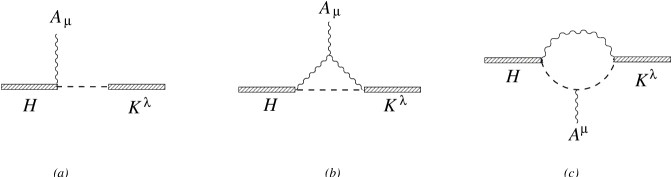
Figure 3: The diagrammatic expression of Eq. (A13): The lowest order term (a) and the one-loop contributions (b and c).

References

(1)
A. Gonzalez-Arroyo and M. Okawa, Phys. Lett. B120, 174 (1983).
(2)
T. Filk, Phys. Lett. B376, 53 (1996).
(3)
C. P. Martin and D. Sanchez-Ruiz, Phys. Rev. Lett. 83, 476 (1999).
(4)
M. M. Sheikh-Jabbari, JHEP 06, 015 (1999);
Phys. Lett. B455, 129 (1999).
(5)
T. Krajewski and R. Wulkenhaar, Int. J. Mod. Phys. A15, 1011 (2000).
(6)
D. Bigatti and L. Susskind, Phys. Rev. D62, 066004 (2000).
(7)
J. M. Maldacena and J. G. Russo, JHEP 09, 025 (1999).
(8)
S. Iso, H. Kawai, and Y. Kitazawa, Nucl. Phys. B576, 375 (2000).
(9)
G. Arcioni and M. A. Vazquez-Mozo, JHEP 0001, 028 (2000).
(10)
S. Minwalla, M. Van Raamsdonk, and N. Seiberg, JHEP 02, 020 (2000).
(11)
I. Y. Aref’eva, D. M. Belov, and A. S. Koshelev, Phys. Lett. B476, 431
(2000).
(12)
D. J. Gross, A. Hashimoto, and N. Itzhaki, Adv. Theor. Math. Phys. 4,
893 (2000).
(13)
A. Matusis, L. Susskind, and N. Toumbas, JHEP 12, 002 (2000).
(14)
M. Hayakawa, hep-th/9912167 (1999);
M. Hayakawa, Phys. Lett. B478, 394 (2000).
(15)
H. O. Girotti, M. Gomes, V. O. Rivelles, and A. J. da Silva, Nucl. Phys. B587, 299 (2000);
hep-th/0102101 (2001).
(16)
D. Zanon, Phys. Lett. B502, 265 (2001);
B504, 101 (2001).
(17)
A. K. Das and M. M. Sheikh-Jabbari, JHEP 06, 028 (2001).
(18)
V. V. Khoze and G. Travaglini,
JHEP 0101, 026 (2001).
(19)
A. Armoni,
Nucl. Phys. B 593, 229 (2001)
[arXiv:hep-th/0005208].
(20)
F. R. Ruiz, Phys. Lett. B 502, 274 (2001).
(21)
H. Liu and J. Michelson, Nucl. Phys. B 614, 279 (2001).
(22)
M. Van Raamsdonk,
JHEP 0111, 006 (2001)
[arXiv:hep-th/0110093].
(23)
A. Bichl, J. Grimstrup, H. Grosse, L. Popp, M. Schweda and R. Wulkenhaar,
JHEP 0106, 013 (2001)
[arXiv:hep-th/0104097].
(24)
For a recent review with a complete list of references see,
for example, M. R. Douglas and N. A. Nekrasov, hep-th/0106048.
(25)
H. J. Grönewold, Physica 12, 405 (1946).
(26)
J. E. Moyal, Proc. Cambridge Phil. Soc. 45, 99 (1949).
(27)
J. I. Kapusta, Finite Temperature Field Theory (Cambridge University
Press, Cambridge, England, 1989).
(28)
M. L. Bellac, Thermal Field Theory (Cambridge University Press,
Cambridge, England, 1996).
(29)
A. Das, Finite Temperature Field Theory (World Scientific, NY, 1997).
(30)
N. K. Nielsen, Nucl. Phys. B101, 173 (1975).
(31)
R. Kobes, G. Kunstatter, and K. W. Mak, Z. Phys. C45, 129 (1989).
(32)
F. T. Brandt and J. Frenkel, Phys. Rev. D56, 2453 (1997).
(33)
H. A. Weldon, Annals Phys. 271, 141 (1999).
(34)
J. C. Taylor,
Nucl. Phys. B 33, 436 (1971);
A. A. Slavnov,
Theor. Math. Phys. 10, 89 (1972)
[Teor. Mat. Fiz. 10153, (1972)].
(35)
M. M. Sheikh-Jabbari, Phys. Rev. Lett. 84, 5265 (2000).
(36)
G. ’t Hooft and M. Veltman, Nucl. Phys. B44, 189 (1972);
C. G. Bollini and J. J. Giambiagi, Nuovo Cim. 12B, 20 (1972).
(37)
I. S. Gradshteyn and M. Ryzhik, Tables of Integral Series and Products
(Academic, New York, 1980).
(38)
F. T. Brandt and J. Frenkel, Phys. Rev. D60, 107701 (1999).
(39)
J. Gomis and T. Mehen, Nucl. Phys. B591, 265 (2000);
O. Aharony, J. Gomis and T. Mehen,
JHEP 0009, 023 (2000) [arXiv:hep-th/0006236].
(40)
L. Alvarez-Gaume, J. L. F. Barbon, and R. Zwicky, JHEP 05, 057 (2001).
(41)
N. Seiberg, L. Susskind, and N. Toumbas, JHEP 06, 021 (2000).
(42)
A. Bassetto, L. Griguolo, G. Nardelli and F. Vian, JHEP 0107, 008 (2001).
(43)
R. Kobes, G. Kunstatter, and A. Rebhan, Phys. Rev. Lett. 64,
2992 (1990); Nucl. Phys. B355, 1 (1991).
(44)
W. Fischler, J. Gomis, E. Gorbatov, A. Kashani-Poor, S. Paban and P. Pouliot,
JHEP 0005, 024 (2000)
[arXiv:hep-th/0002067].
(45)
S. S. Gubser and S. L. Sondhi, Nucl. Phys. B605, 395 (2001).
(46)
L. Griguolo and M. Pietroni, hep-th/0102070 (2001).