Unrenormalizable Theories Can Be Predictive.

Abstract

Unrenormalizable theories contain infinitely many free parameters. Considering these theories in terms of the Wilsonian renormalization group (RG), we suggest a method for removing this large ambiguity. Our basic assumption is the existence of the maximal ultraviolet cutoff in a cutoff theory, and we require that the theory be so fine-tuned as to reach the maximal cutoff. The theory so obtained behaves as a local continuum theory to the shortest distance. In concrete examples of the scalar theory we find that at least in a certain approximation to the Wilsonian RG, this requirement enable us to make unique predictions in the infrared regime in terms of a finite number of independent parameters. Therefore, the method might provide a way for calculating quantum corrections in a low-energy effective theory of quantum gravity.

I Introduction

Quantum field theories are classified according to their renormalizability. Needless to say that not only renormalizable, but also unrenormalizable theories have played important rôle in particle physics [1]. It is however widely accepted that an unrenormalizable theory is only a low-energy effective theory of a more fundamental theory. The low-energy effective theory should contain the correct low-energy degrees of freedom of the fundamental theory, and it should be possible, within the framework of the effective theory, to compute approximate low-energy quantum processes of the fundamental theory.

If the effective theory is perturbatively unrenormalizable, we face a serious problem. How many independent parameters should have the perturbatively unrenormalizable theory? The answer in perturbation theory is: Infinitely many, by definition. Of course, this does not prevent from applying perturbation theory to unrenormalizable theories to make predictions, as in chiral perturbation theory which has a certain success [2, 3, 4]. Nevertheless we may ask why chiral perturbation theory has so many independent parameters at the quantum level, although it is the effective theory of QCD. This large ambiguity cannot be controlled by a symmetry [2, 3], and we are concerned with this problem which always exists in unrenormalizable effective theories. In this paper, we propose to remove this large ambiguity within the framework of the effective theory.

The idea is based on a simple intuitive picture. Suppose we formulate both a fundamental theory and its low-energy effective theory in terms of the Wilsonian renormalization group (RG) [5]. We assume that the effective theory is a cutoff theory. Since we assume that the fundamental theory is free from the ultraviolet cutoff, $\Lambda_{0}$, we can let go $\Lambda_{0}$ to infinity. That is, starting at some point in the infrared regime, the RG flow in the fundamental theory evolves along a renormalized trajectory, and approaches an ultraviolet fixed point in the ultraviolet limit. The flow has to evolve for “infinite time” to arrive at the fixed point [5]. The RG flow in the effective theory that evolves for the “ maximal time” may be the best approximation to the renormalized trajectory of the fundamental theory, and the effective theory along that trajectory behaves as a local continuum theory down to the shortest distance. The large ambiguity of the cutoff theory could be removed in this way. In Sec. II we will formulate our idea.

We will consider the scalar theory in four, five and six dimensions in Sec. III, and apply our idea to these theories. It will be shown that in lower orders in our approximation to the Wilsonian RG, the ambiguities inherent in these theories can be removed. We will also argue that the ambiguity in four dimensions, which we will fix, is the renormalon ambiguity [6, 7]. Einstein’s theory of gravity and also Yang-Mills theories in more than four dimensions are perturbatively unrenormalizable, and the conventional method of perturbation theory loses its power in these theories . The application to quantum gravity and also higher-dimensional Yang-Mills theories would go beyond the scope of this paper, and we leave it to feature work. However, as far as renormalization is concerned, the scalar theory in more than four dimensions may be seen as an oversimplified model of a low-energy effective theory of quantum gravity [8] .

We conclude in Sec. IV, and the explicit expressions for the $\beta$ functions which we use in an approximation scheme that is specified in Sec. III are given in Appendix.

II Making unrenormalizable theories predictive.

Our interest is directed to field theories [5] which become weakly coupling in the infrared regime. These theories can be perturbatively renormalizable or unrenormalizable. Suppose we consider such a theory in terms of the Wilsonian RG [5]. We then gradually increase the ultraviolet cutoff $\Lambda_{0}$ while keeping fixed the values of the coupling constants of the theory at some point $\Lambda$ in the infrared regime, and consider the RG flow as a function of $\Lambda_{0}$. In the case of a nontrivial theory, the ultraviolet cutoff $\Lambda_{0}$ can become infinite, and the RG flow converges to a fixed point, if a certain set of the coupling constants is exactly fine tuned at $\Lambda$, that is, if they lie exactly on a renormalized trajectory [5]. If the theory is trivial, $\Lambda_{0}$ cannot become infinite, or the RG flow does not converge to a point. Suppose there exists the maximal value $\Lambda_{\rm max}$ in the theory. To reach $\Lambda_{\rm max}$, we have to fine tune the values of the coupling constants at $\Lambda$ as in the case of a nontrivial theory.

With this observation, we now come to formulate our method under the basic assumption that there exists the maximal value of the ultraviolet cutoff $\Lambda_{\rm max}$ in a theory. If the theory is perturbatively renormalizable, there should be a set of dimensionless coupling constants. In this case we regard all the coupling constants with a canonical dimension $<0$ as dependent coupling constants. If the theory is perturbatively unrenormalizable, there should exist a set of coupling constants with a negative canonical dimension $\geq d_{\rm max}$, which should be regarded as independent. In this case we regard all the coupling constants with a canonical dimension $<d_{\rm max}$ as dependent coupling constants. With this classification of the independent and dependent coupling constants, we then require from the dependent coupling constants that for given values of the independent coupling constants in the infrared regime, the dependent ones are so fine tuned that one arrives at the maximal value of the ultraviolet cutoff .

Polchinski [13] investigated the Wilsonian RG flow of the scalar theory in four dimensions to show its perturbative renormalizability . His observation, assuming that the mass parameter can be neglected, is that there exists a trajectory in the space of coupling constants, which is attractive in the infrared limit. That is, whatever the initial values of the coupling constants at $\Lambda_{0}$ are, they converge to the trajectory, if the $\Lambda_{0}$ is large enough. This is then interpreted as perturbative renormalizability. Therefore, in the class of theories, in which Polchinski’s criterion on perturbative renormalizability can be applied, the ultraviolet cutoff $\Lambda_{0}$ should be sufficiently large so that physics in the infrared regime has less dependence of the initial values of the coupling constants at $\Lambda_{0}$. It should be therefore assumed for perturbative renormalization to work in those trivial, but perturbatively renormalizable theories that the intrinsic cutoff of the theory is so large that the nonperturbative effects due to the finite intrinsic cutoff are very small in the infrared regime . If the intrinsic cutoff is low, the initial value ambiguities are not sufficiently suppressed in the infrared regime, and consequently the perturbative calculations may not be reliable. Therefore, the intrinsic cutoff can be much larger than the actual physical cutoff at which a new physics enters. As for these perturbative renormalizable theories, our requirement is a slight extension of the requirement in perturbative renormalization; the maximal, instead of a large, cutoff is assumed.

According to Polchinski [13], we interpret a theory as perturbatively unrenormalizable, if there is no infrared attractive trajectory (or no infrared attractive subspace of a finite dimension). Physics in the infrared regime in this case depends on the initial values of the infinitely many coupling constants at $\Lambda_{0}$. This is exactly the situation which we are more interested in. Although in the case of perturbative renormalizable theories, our requirement of the maximal cutoff is a slight extension, this requirement, applied to a perturbatively unrenormalizable theory, could select a trajectory out the infinitely many trajectories. The theory along this trajectory will behave as a local continuum theory to the shortest distance. In the next section we will consider concrete unrenormalizable theories, and see that our idea works at least in a certain approximation. If our idea could be founded in a more rigorous manner, it could be promoted to a principle, which we would like to call principle of maximal locality. It is, however, beyond the scope of the present paper to do this task.

III Application to the scalar theory
in diverse dimensions

A Continuous Wilsonian renormalization group

As we have explained in detail in Sec. II, our interest is directed to trivial theories. To define such theories in a nonperturbative fashion, we have to introduce a cutoff. A natural framework to study cutoff theories is provided by the continuous Wilsonian RG [5][12]–[15]. Let us briefly illustrate the basic idea of the Wilsonian RG approach in the case of the $N$ component scalar theory in euclidean $d$ dimensions . One divides the field $\phi(p)$ in the momentum space into low and high energy modes according to

$$\phi^{k}(p)=\theta(|p|-\Lambda)~{}\phi_{>}^{k}(p)+\theta(\Lambda-|p|)~{}\phi_{<}^{k}(p)~{},~{}k=1,\dots,N~{}.$$ (1)

The Wilsonian effective action is then defined by integrating out only the high energy modes in the path integral:

$$S_{\rm eff}[~{}\phi_{<},\Lambda~{}]=-\ln\left\{\int{\cal D}\phi_{>}~{}e^{-S[\phi_{>},\phi_{<}]}\right\}.$$ (2)

It was shown in Refs. [5, 12] that the path integral corresponding to the difference

$$\delta S_{\rm eff}=S_{\rm eff}[~{}\phi_{<},\Lambda+\delta\Lambda~{}]-S_{\rm eff}[~{}\phi_{<},\Lambda~{}]$$ (3)

for an infinitesimal $\delta\Lambda$ can be exactly carried out, yielding the RG evolution equation of the effective action

$$\frac{\partial S_{\rm eff}}{\partial t} = -\Lambda\frac{\partial S_{\rm eff}}{\partial\Lambda}={\cal O}(S_{\rm eff})~{},$$ (4)

where ${\cal O}$ is a non-linear operator acting on the functional $S_{\rm eff}$. There exist various (equivalent) formulations [12]–[15], but in this paper we consider only the Wegner-Houghton (WH) equation [12]. Since $S_{\rm eff}$ is a functional of fields, one can think of the WH equation as coupled differential equations for infinitely many couplings in the effective action. The crucial point is that ${\cal O}$ can be exactly derived for a given theory, in contrast to the perturbative RG approach where the RG equations are known only up to a certain order in perturbation theory. This provides us with possibilities to use approximation methods that go beyond the conventional perturbation theory.

In the derivative expansion approximation [17, 14]-[18]-[20], one assumes that the effective action $S_{\rm eff}[\phi,\Lambda]$ can be written as a space-time integral of a (quasi) local function of $\phi$, i.e.,

$$S_{\rm eff}[\phi,\Lambda] = \int d^{d}x\,(\,\frac{1}{2}\,\sum_{k,l=1}^{N}\partial_{\mu}\phi^{k}\partial_{\mu}\phi^{l}\,Z^{kl}(\phi,\Lambda)+V(\phi,\Lambda)+\dots~{})~{},$$ (5)

where $\dots$ stands for terms with higher order derivatives with respect to the space-time coordinates. In the lowest order of the derivative expansion (the local potential approximation [17, 14]), there is no wave function renormalization ($Z^{kl}(\phi,\Lambda)=\delta^{kl}$), and the RG equation for the effective potential $V$ can be obtained. Since it is more convenient to work with the RG equation for dimensionless quantities, which makes the scaling properties more transparent, we rescale the quantities according to

$$p \to\Lambda p~{},~{}\phi^{k}\to\Lambda^{d/2-1}\phi^{k}~{},~{}V\to\Lambda^{d}V~{}.$$ (6)

Then the RG equation $V(\phi,\Lambda)$ is given by [14]

$$\frac{\partial V}{\partial t} = -\Lambda\frac{\partial V}{\partial\Lambda}=a~{}\ln(1+V^{\prime}+2\rho V^{\prime\prime})+a(N-1)\ln(1+V^{\prime})+dV+(2-d)\rho V^{\prime}~{},$$ (7)

where the prime on $V$ stands for the derivative with respect to $\rho$, and

$$\rho = \frac{1}{2}\sum_{k=1}^{N}\phi^{k}\phi^{k}~{},~{}a=\frac{1}{2^{d}\pi^{d/2}\Gamma(d/2)}~{}.$$ (8)

Eq. (7) ( or the one which is derived from (7) for $F=V^{\prime}=\partial V/\partial\rho$) is the central equation we will analyze in the following subsections. Therefore, all the results we will obtain are valid only within the local potential approximation. There are however no fundamental problems in going beyond this approximation.

B Toy model in $d=3$

The scalar theory in $d=3$ dimensions have a nontrivial fixed point, Wilson-Fisher fixed point [5], and is moreover asymptotically free. So this theory is nontrivial as it is well known, and therefore lies outside of our interest. However, we would like to consider this theory with infrared and ultraviolet interchanged in order to illustrate what we mean by “ being closest to a nontrivial theory”. So, the results obtained here will be compared with those of trivial theories which we will consider later.

The interchange of infrared and ultraviolet just means the replacement $t\to-t$. We then consider $F=V^{\prime}=\partial V/\partial\rho$ for $N=1$, and derive the evolution equation from (7) for $F$

$$\frac{\partial F}{\partial t} = -2F+\rho F^{\prime}-a~{}\frac{3F^{\prime}+2\rho F^{\prime\prime}}{1+F+2\rho F^{\prime}}~{},~{}a=\frac{1}{4\pi^{2}}~{}.$$ (9)

The power series ansatz

$$F(\rho,t) = 4a~{}f_{0}(t)+\sum_{n=1}^{\infty}f_{n}(t)~{}[\frac{\rho}{4a}]^{n}$$ (10)

defines the coupling constants $f_{n}$, and Eq. (9) gives a set of $\beta$ functions which in lower orders in the expansion are given by

$$\beta_{0} = \frac{df_{0}}{dt}=-2f_{0}-\frac{3}{4}\frac{f_{1}}{(1+f_{0})}~{},$$ (11)

$$\beta_{1} = \frac{df_{1}}{dt}=-f_{1}+\frac{9}{4}\frac{f_{1}^{2}}{(1+f_{0})^{2}}~{},$$ (12)

Where we have made a truncation at $n=1$ above. There exist two fixed points

$$(f_{0}=0,f_{1}=0)~{},~{}(f_{0}=-\frac{1}{7},f_{1}=\frac{16}{49})~{}.$$ (13)

All the directions from the Gaussian fixed point (at this level of truncation) are infrared stable; the eigenvalues are $(-1,-2)$ with the corresponding eigenvectors $(-3/4,1)$ and $(1,0)$, respectively. The solution near the origin can easily be found:

$$f_{0} = -\frac{3}{4}f_{1}+[~{}C-\frac{27}{16}\log(f_{1})~{}]f_{1}^{2}+O(f_{1}^{3})~{},$$ (14)

where $C$ is an integration constant. The solution is obtained from $df_{0}/df_{1}=\beta_{0}/\beta_{1}$. At this stage, $f_{0}$ and $f_{1}$ behave independently. Note that there is a certain infrared attractiveness, because $f_{0}$ approaches to a definite function, $-(3/4)f_{1}$, in the infrared limit $f_{1}\to 0$.

The integration constant $C$ can be determined by requiring that the RG flow approaches to the ultraviolet fixed point $(f_{0}=-1/7,f_{1}=16/49)$. That is, the coupling constant $f_{0}$ has to be exactly fine tuned for the ultraviolet cutoff $\Lambda_{0}$ to become infinite. If $f_{0}$ is not exactly fine tuned, the RG flow runs into infinity at some finite $\Lambda_{0}$. The fine-tuning procedure is shown in Fig. 1 for $f_{1}=0.01$ at $t=0$, where the vertical axis is $T_{0}=\log\Lambda_{0}/\Lambda$ and the horizontal one is $f_{0}(0)$. From Fig. 1 we find that in this case $f_{0}$ at $t=0$ should be fine tuned at $-0.00718\ldots$.

C $d=4$: Perturbatively renormalizable case

We now come to discuss a trivial, but perturbatively renormalizable case . In this case, our interest focuses on the nonperturbative ambiguity that results from the fact that perturbation series diverge. There are rigorous results that this divergence is dominated by the renormalon singularity in the Borel plane, and the form of the ambiguity is known [6]. Since the Wilsonian RG is nonperturbative, it is natural to assume that it also contains this information. Of course, it is not clear that one can see it within the framework of our approximation. We will argue, based on our numerical analysis, that this is the case.

As in the case for $d=3$, we consider the derivative $F=\partial V/\partial\rho=V^{\prime}$, where the potential $V$ is assumed to be expandable as

$$V(\rho,t) = v_{0}(t)+\sum_{n=1}^{\infty}\frac{1}{n+1}\frac{f_{n}(t)}{(4a)^{n}}~{}[~{}\rho-4af_{0}(t)~{}]^{n+1}~{}$$ (15)

$$= v_{0}(t)+\frac{1}{2}\frac{f_{1}(t)}{4a}[~{}\frac{1}{2}{\bf\phi}\cdot{\bf\phi}-4af_{0}(t)~{}]^{2}+\frac{1}{3}\frac{f_{2}(t)}{(4a)^{2}}[~{}\frac{1}{2}{\bf\phi}\cdot{\bf\phi}-4af_{0}(t)~{}]^{3}+\cdots~{}.$$ (16)

The constant $a$ is given in (7) ($a(d=4)=1/16\pi^{2}$), and $\rho={\bf\phi}\cdot{\bf\phi}/2=\sum_{i=1}^{N}\phi_{i}\phi_{i}/2$. Here we have shifted $\rho$ by $4af_{0}(t)$ from the reason we will give soon. The squared mass is $2f_{0}f_{1}$ so that if $\lim_{t\to\infty}2f_{0}(t)f_{1}(t)~{}>(<)~{}0$, we are in the (un)broken phase, and the critical surface is defined by the RG flows that satisfy $\lim_{t\to\infty}2f_{0}(t)f_{1}(t)=0$. Inserting the power series ansatz (15) into the evolution equation for $F$

$$\frac{\partial F}{\partial t} = 2F+(2-d)\rho F^{\prime}+a\left[~{}\frac{3F^{\prime}+2\rho F^{\prime\prime}}{1+F+2\rho F^{\prime}}+(N-1)\frac{F^{\prime}}{1+F}~{}\right]~{},$$ (17)

we can obtain the $\beta$ functions, $\beta_{n}=df_{n}/dt$, at any finite order of truncation. (The explicit expressions in lower orders are given in Appendix A.) One can convince oneself that the $n$th order $\beta$ function has the form

$$\beta_{n} = (2+2n-nd)f_{n}+\sum_{i_{1}+2i_{2}+\cdots+ni_{n}=n+1}~{}\eta_{i_{1}\cdots i_{n}}~{}f_{1}^{i_{1}}\cdots f_{n}^{i_{n}}$$ (19)

$$+\sum_{l=1}^{n+1}\sum_{m=0}^{n+1}\left[\sum_{-i_{l0}+\cdots+mi_{lm}=n+1}~{}\chi^{(l)}_{i_{l0}\cdots i_{lm}}~{}f_{0}^{i_{l0}}f_{1}^{i_{l1}}\cdots f_{m}^{i_{lm}}~{}\Delta^{l}\right]~{},$$

where

$$\Delta=(1+2f_{0}f_{1})^{-1}~{}.$$ (20)

Given the $\beta$ functions, we investigate the infrared and ultraviolet behavior of the theory, and we first investigate the infrared behavior for

$$d = 4~{}~{}\mbox{and}~{}~{}N=4~{}.$$ (21)

Obviously, ($f_{0}=3/4~{},~{}f_{n}=0~{}(n\geq 1)$) is a fixed point (Gaussian fixed point). The stability of the RG flows near the Gaussian fixed point cannot be simply discussed in the present case, because the $\beta$ functions are singular at this point ($1/f_{1}$ which is present in $\beta_{0}$ appears in other $\beta$ functions). So we construct explicitly the solution near the Gaussian fixed point to investigate its stability. To this end, we eliminate $t$ in favor of $f_{1}$ using the set of equations

$$\beta_{1}\frac{df_{n}}{df_{1}} = \beta_{n}~{},~{}(n\neq 1)~{},$$ (22)

which is called the reduction equation in Ref. [23]. We find that the power series solution

$$f_{0} = \frac{3}{4}+\sum_{l=0}^{\infty}C^{(l)}_{0}f_{1}^{l+1}~{},$$ (23)

$$f_{n} = f_{1}^{n+1}\sum_{l=0}^{\infty}C^{(l)}_{n}f_{1}^{l}~{}$$ (24)

exists. That is, the expansion coefficients can be uniquely computed for a given truncation of the series (15). Using this power series solution, we obtain the general solutions that surround this special solution by solving the linearized equations

$$-3f_{1}^{2}\frac{d\delta f_{0}}{df_{1}} \simeq 2\delta f_{0}-\frac{3}{4f_{1}}\delta f_{2}~{},$$ (25)

$$-3f_{1}^{2}\frac{d\delta f_{n}}{df_{1}} \simeq [~{}(2-2n)-3p_{n}f_{1}~{}]\delta f_{n}+\sum_{i\neq n}q_{(}f_{1})\delta f_{i}~{}.$$ (26)

Therefore, the integration constant $K_{n}$ of $\delta f_{n}$ appears in the exponential form

$$K_{n}\exp(\frac{2-2n}{3f_{1}})~{}f_{1}^{p_{n}}~{},$$ (27)

where $p_{n}$ are fractional numbers. We find that for $n\leq 2$

$$f_{0} = \frac{3}{4}-\frac{9}{16}f_{1}^{2}+\frac{225}{64}f_{1}^{2}-\frac{7857}{256}f_{1}^{3}+\frac{269001}{1024}f_{1}^{4}-\frac{12806991}{4096}f_{1}^{5}+\frac{650870883}{16384}f_{1}^{6}+O(f_{1}^{7})$$ (29)

$$+K_{2}\exp(-\frac{2}{3f_{1}}-\frac{57}{4}f_{1})~{}f_{1}^{7/2}~{}[\frac{3}{16}-\frac{9}{8}f_{1}+\frac{2799}{256}f_{1}^{2}+O(f_{1}^{3})~{}]~{},$$

$$f_{2} = \frac{15}{4}f_{1}^{3}-\frac{189}{8}f_{1}^{4}+\frac{7479}{64}f_{1}^{5}-\frac{12879}{32}f_{1}^{6}+O(f_{1}^{7})+K_{2}\exp(-\frac{2}{3f_{1}}-\frac{57}{4}f_{1})~{}f_{1}^{9/2}~{}.$$ (30)

Note that there is no independent integration constant for $f_{0}$. The general solutions define a $n$-dimensional hypersurface in the space of $n+1$ coupling constants, which is nothing but the critical surface. We see from (27) that thanks to the exponential function $\exp[(2-2n)/3f_{1}]$ the deviations $\delta f_{n}$ from the power series solutions vanish very fast as $f_{1}$ approaches zero, implying that the power series solutions (23) and (24) are very attractive in the infrared limit. This infrared attractiveness is interpreted as perturbative renormalizability by Polchinski [13, 24]. We adapt to his interpretation, and call these solutions the perturbative solutions . The exponential deviations defined in (26) are therefore nonperturbative contributions, which cannot be computed usually [7]. So we call them a nonperturbative ambiguity as in Ref. [7].

Before we proceed, we would like to argue that the nonperturbative ambiguity we mentioned above results from the fact that perturbation series diverge, that is, it is the renormalon ambiguity [6]. We have computed higher orders in the power series expansion (30) and found that they do not approximate the exact (numerical) result better. The one with the first four terms in (30) is the best approximation among lower orders. From this fact, we believe that the power series solution (30) does not converge, and that it is an asymptotic series. So, the power series (30) reflects the property of perturbation series in the conventional perturbation theory, as far as our numerical analysis in lower orders suggests. This is one of the reasons why we interpret the power series as the perturbative series. This interpretation is also supported by the fact that not only the leading form of the nonperturbative ambiguity, the last exponential term in (30), agrees with that of the known renormalon ambiguity [6], but also the coefficient of $1/f_{1}$, $2/3$, in the exponential function. The power of $f_{1}$ in front of the exponential function, that is $9/2$, differs slightly from the expected value $3$. The origin is presumably the local potential approximation to the exact RG evolution equation. Therefore, we believe that the last term in (30) is the renormalon ambiguity. As we will see, we can remove this ambiguity by requiring the maximal cutoff.

Off the critical surface (defined by (29) and (30)), $f_{0}$ increases in the infrared limit, and approaches infinity. We would like to solve the reduction equation (22) in this limit. To this end, we consider the evolution of $m^{2}=2f_{0}f_{1}$ (the mass squared in the broken phase) and find that it also increases in the limit. Therefore, in the lowest order, we just have to solve

$$-\frac{3}{4}f_{1}^{2}\frac{df_{n}}{df_{1}} \simeq (-1)^{n}\frac{3}{4}f_{1}^{n+1}+(2-2n)f_{n}~{},$$ (31)

and obtain for instance

$$f_{2} \simeq -\frac{4}{3}f_{1}-\frac{1}{2}f_{1}^{2}+\frac{32}{9}\exp(-\frac{8}{3f_{1}})Ei(\frac{8}{3f_{1}})+\hat{K}_{2}\exp(-\frac{8}{3f_{1}})~{}.$$ (32)

The solution becomes a power series in $f_{1}$, if the integration constant $\hat{K}_{2}$ is set equal zero:

$$f_{2} = \frac{3}{8}f_{1}^{3}+\frac{9}{8}f_{1}^{4}+\cdots$$ (33)

So the last term in (32) exhibits the nonperturbative ambiguity, which we will compute by requiring the maximal cutoff later on.

To proceed, we would like to study the ultraviolet behavior of the theory, and consider the general form of the $\beta$ functions (19) as well as the explicit form for $\beta_{0}$ and $\beta_{1}$ (given in (A1)–(A13)) along with the reduction equation (22). To solve (22), we assume that $|f_{n}|~{}~{}(n\geq 2)$ increases as $f_{1}$ increases, while $f_{0}$ remains finite in the limit. It follows that under this assumption, the coupling constants have the leading behavior

$$f_{0} = J_{0}^{(0)}+J_{0}^{(1)}/f_{1}+O(f_{1}^{-2})~{},$$ (34)

$$f_{n} = J_{n}^{(0)}f_{1}^{n}+O(f_{1}^{n-1})~{},~{}(n\geq 2)~{}.$$ (35)

The coefficient $J_{0}^{(0)}$ cannot be determined, while the others can be uniquely computed as functions of $J_{0}^{(0)}$. At $n=3$ for instance we find

$$J_{0}^{(1)} = \frac{-3+8J_{0}^{(0)}-2J_{2}^{(0)}}{3+8(J_{2}^{(0)})^{2}-6J_{3}^{(0)}}~{},$$ (36)

$$J_{2}^{(0)} = \left\{\begin{array}[]{c}-1.2186\cdots\\ 0.3722\cdots\end{array}\right.~{},~{}J_{3}^{(0)}=\left\{\begin{array}[]{c}0.8382\cdots\\ 0.2329\cdots\end{array}\right.~{}~{}\mbox{for}~{}~{}\left\{\begin{array}[]{c}\mbox{broken phase}\\ \mbox{unbroken phase}\end{array}\right.~{}.$$ (43)

The leading behavior given by (34) and (35) is stable in the ultraviolet limit at least for $n\leq 3$. To show this, we construct the general solutions that surround the lading behavior (34) and (35) in the ultraviolet limit, and denote the deviations from the leading behavior by $\delta f_{n}$. We first find

$$\frac{d\delta f_{0}}{df_{1}} \simeq -r_{0}\frac{\delta f_{0}}{f_{1}^{2}}~{},r_{0}\simeq\left\{\begin{array}[]{c}0.538\\ 1.95\end{array}\right.~{}~{}\mbox{for}~{}~{}\left\{\begin{array}[]{c}\mbox{broken phase}\\ \mbox{unbroken phase}\end{array}\right.~{}.$$ (48)

This implies that the leading order deviation $\delta f_{0}$ is just a shift of the undetermined constant $J_{0}^{(0)}$, which we denote by $\delta J_{0}^{(0)}$. For $\delta f_{2,3}$, we find

$$\left(\begin{array}[]{c}\frac{d\delta f_{2}}{df_{1}}\\ \frac{d\delta f_{3}}{df_{1}}\end{array}\right) \simeq \left(\begin{array}[]{cc}-4.98/f_{1}~{},\ -2.95/f_{1}^{2}\\ -9.57~{},\ -3.98/f_{1}\end{array}\right)\left(\begin{array}[]{c}\delta f_{2}\\ \delta f_{3}\end{array}\right)+\delta J_{0}^{(0)}\left(\begin{array}[]{c}4.02/(J_{0}^{(0)})^{2}\\ 5.72f_{1}/(J_{0}^{(0)})^{2}\end{array}\right)$$ (57)

for the broken phase. Similarly, we find that for the unbroken phase

$$\left(\begin{array}[]{c}\frac{d\delta f_{2}}{df_{1}}\\ \frac{d\delta f_{3}}{df_{1}}\end{array}\right) \simeq \left(\begin{array}[]{cc}0.302/f_{1}~{},\ 3.26/f_{1}^{2}\\ -1.03~{},\ 1.30/f_{1}\end{array}\right)\left(\begin{array}[]{c}\delta f_{2}\\ \delta f_{3}\end{array}\right)+\delta J_{0}^{(0)}\left(\begin{array}[]{c}0.0697/(J_{0}^{(0)})^{2}\\ 0.0491f_{1}/(J_{0}^{(0)})^{2}\end{array}\right)~{}.$$ (66)

The corresponding solutions are found to be

$$\delta f_{2} \simeq \left\{\begin{array}[]{l}0.101(\eta_{a}+\eta_{b})\delta J_{0}^{(0)}f_{1}/(J_{0}^{(0)})^{2}+\eta_{a}f_{1}^{-10.3}+\eta_{b}f_{1}^{0.329}\\ \\ 0.0185(\eta_{c}+\eta_{d})\delta J_{0}^{(0)}f_{1}/(J_{0}^{(0)})^{2}+f_{1}^{0.302}[~{}\eta_{c}\cos(1.83\ln f_{1})\\ +\eta_{d}\sin(1.83\ln f_{1})~{}]\end{array}\right.~{},$$ (71)

$$\delta f_{3} \simeq \left\{\begin{array}[]{l}1.19(\eta_{a}+\eta_{b})\delta J_{0}^{(0)}f_{1}^{2}/(J_{0}^{(0)})^{2}+1.80[\eta_{a}f_{1}^{-9.30}+\eta_{b}f_{1}^{1.33}]\\ \\ -0.0231(\eta_{c}+\eta_{d})\delta J_{0}^{(0)}f_{1}^{2}/(J_{0}^{(0)})^{2}-0.562f_{1}^{1.30}[~{}\eta_{c}\sin(1.83\ln f_{1})\\ -\eta_{d}\cos(1.83\ln f_{1})~{}]\end{array}\right.$$ (76)

for the broken and unbroken phases, respectively. Therefore, $\lim_{f_{1}\to\infty}\delta f_{2}/f_{2}=\lim_{f_{1}\to\infty}\delta f_{3}/f_{3}=0$, implying that the leading behavior (34) and (35) is stable, and that the coupling constants $f_{2}$ and $f_{3}$ (which have a negative canonical dimension before they were made dimensionless) diverge at the same scale $\Lambda_{0}$ at which $f_{1}$ diverges. This feature presumably continues to higher order truncations. That is, all the coupling constants $f_{n}~{}~{}(n\geq 1)$ diverge at the common scale. But whether our method works or not does not depend on it.

At this stage we would like to explain why we have shifted $\rho$ in the ansatz (15). The reason is the following. $f_{0}$ approaches a finite, undetermined constant $J_{0}^{(0)}$ in the ultraviolet limit so that the propagator effect $\Delta$ (given in (20) ) which appears in the $\beta$ functions $\beta_{n}$ is finite for any positive $f_{1}$ in the ultraviolet limit. This makes the numerical analysis in the ultraviolet limit easier, while without the shift in the unbroken case $\Delta=(1+m^{2})^{-1}$ may easily become singular for some finite positive $f_{1}$. Of course this complication is not a serious hindrance for applying our method.

According to Sect. II, we regard $f_{0}$ and $f_{1}$ as independent parameters, while the other coupling constants $f_{n}~{}~{}(n\geq 2)$ should be regarded as dependent. We then require that for given values of $f_{0}$ and $f_{1}$ at $\Lambda<<\Lambda_{0}$, all the dependent coupling constants $f_{n}~{}~{}(n\geq 2)$ should be so fine tuned at $\Lambda$ that $f_{n}~{}~{}(n\geq 1)$ diverge at the maximal value of $\Lambda_{0}$. This program cannot be solved analytically, and we relay on numerical analyses. In Fig. 2 we plot the running time $T_{0}=\ln(\Lambda_{0}/\Lambda)$ against $f_{2}(t=0)$ for $f_{0}(0)=1/4a=4\pi^{2}$ and $f_{1}(0)=0.1$ in the case of the truncation at $n=2$. Comparing Fig. 2 with Fig. 1 of the nontrivial case, we observe a similarity, although $T_{\rm max}$ cannot be infinite in the present case. We see that $T_{0}$ is peaked at $f_{2}(0)\simeq 0.000528$. To see the truncation dependence we calculate the fine-tuned value of $f_{2}(0)$ as a function of $f_{1}(0)$ for the truncations at $n=2$ and $3$. The result is plotted in Fig. 3 for the case $f_{0}(0)=1/4a=4\pi^{2}$. The solid and dotted lines correspond to $n=2$ and $3$, respectively. We observe that the result does not depend very much on the order of truncation. The fine-tuned value of $f_{3}(0)$ as a function of $f_{1}(0)$ is plotted in Fig. 4 for $f_{0}(0)=1/4a=4\pi^{2}$.

Now we come to the determination of the coefficient $K_{2}$ in (30), which exhibits a nonperturbative correction of the renormalon type [6, 7]. In Fig. 5 we plot $T_{0}=\ln(\Lambda_{0}/\Lambda)$ against $K_{2}$, and in Fig. 6, $T_{0}$ is plotted against $f_{2}(0)$ at $f_{1}(0)=0.1$. From this result we obtain

$$K_{2} \simeq 7\times 10^{3}~{}.$$ (77)

This means a departure of about $3~{}(0.1)$ % from the perturbative result at $f_{1}=0.1~{}(0.07)$. Needless to say that the corresponding effect in the standard model could be in principle measurable.

At last we would like to compare the maximal running time $T_{\rm max}$ obtained in perturbation theory with our nonperturbative value. To this end, we use the perturbative evolution equation

$$\frac{\partial f_{1}}{\partial t} = -3f_{1}^{2}~{},$$ (78)

and obtain $T_{\rm max}=10/3\simeq 3.3$, which should be compared with the nonperturbative result in Figs. 5 and 6.

These results obtained above show that our method works in the four-dimensional case. It is certainly possible to formulate our idea in terms of lattice theory. Then one could improve the accuracy of the calculation of $K_{2}$.

D $d=5,6$: Perturbatively unrenormalizable cases

We now come to discuss unrenormalizable cases :

$$d=5,6~{}~{}\mbox{and}~{}~{}N=4~{}.$$ (79)

We emphasize that as far as renormalization is concerned, and we are interested in the infrared regime, the scalar theory in five or higher dimensions may be seen as an oversimplified model of a low-energy effective theory of quantum gravity [8].

As in the case for $d=4$, we consider the derivative $F=V^{\prime}$, and follow basically the investigations of that case. The calculations for the $d=6$ case are the same as for the $d=5$ case, and therefore, we consider only the $d=5$ case below. So the details for the $d=6$ case are suppressed below, but we give the final result for this case, too, at the end. We first investigate the infrared behavior, and find that the Gaussian point ($f_{0}=1/2~{},~{}f_{n}=0~{}(n\geq 1)$) is a fixed point. As in the previous case, we construct explicitly the solution near the Gaussian fixed point to investigate its stability. We find that the power series solutions like (23) and (24) do not exist. Instead, the expansion of the form (which is similar to (14) in the nontrivial case)

$$f_{0} = \frac{1}{2}-\frac{3}{16}f_{1}+\frac{171}{160}f_{1}^{2}+[~{}\frac{9}{2}\ln f_{1}-\frac{435}{128}+\frac{C_{2}}{12}~{}]~{}f_{1}^{3}-[~{}\frac{54}{7}\ln f_{1}+\frac{554013}{62720}+\frac{C_{2}}{7}~{}]~{}f_{1}^{4}$$ (81)

$$+[~{}\frac{3225933}{250880}+\frac{10441}{8960}C_{2}+\frac{281907}{4480}\ln f_{1}~{}]f_{1}^{5}+O(f_{1}^{6}\ln f_{1})~{},$$

$$f_{2} = f_{1}^{3}\left(\frac{15}{2}+[~{}54\ln f_{1}+C_{2}~{}]~{}f_{1}+[~{}81\ln f_{1}+\frac{3}{2}C_{2}-\frac{9315}{32}~{}]~{}f_{1}^{2}+O(f_{1}^{3}\ln f_{1})\right)~{},$$ (82)

for $d=5$ at the truncation $n=2$ exhibit the general solutions, where $C_{2}$ is an integration constant. As in the case for $d=4$, there is no independent integration constant for $f_{0}$, and the general solutions define the $n$-dimensional critical surface in the space of $n+1$ coupling constants. As $K_{2}$ in (30), we will calculate $C_{2}$ by requiring the maximal cutoff later. The ambiguity expressed by $C_{2}$ in (82) is indeed suppressed by $f_{1}^{4}$ in the infrared limit, but we also see that in contrast to (29) and (30) in $d=4$ dimensions, there are no strong infrared attractive functions like the perturbative solutions (23) and (24). Therefore, following Polchinski [13, 24], the theory is perturbatively unrenormalizable, in accord with the result in perturbation theory.

Whether power series solutions like (23) and (24) exist depends crucially on the existence of a dimensionless coupling constant. Namely, if there is no dimensionless coupling constant, there are no couplings for which the linear term in the $\beta$ function, $(2+2n-nd)f_{n}$ in the case of (19), vanishes. Then the reduction equation (22) becomes

$$d_{x}x\frac{dy}{dx} = d_{y}y$$ (83)

in the vicinity of the Gaussian fixed point, where $x$ and $y$ denote generic coupling constants, and $d_{x}$ and$d_{y}$ are their canonical dimensions before the dimensional rescaling (6). The solution of (83) is simply $y=\tilde{C}x^{d_{y}/d_{x}}$, where $\tilde{C}$ is an integration constant, but one can convince oneself that logarithmic terms such as $x^{d_{y}/d_{x}}\ln x$ are needed to construct a solution of the full problem. This is the origin of the logarithmic terms in (81) and (82), and also in (14). The difference between $C_{2}$ in (82) and $C$ in (14) is that $C$ is determined by nontriviality, while $C_{2}$ will be determined by the maximal cutoff.

Off the critical surface, the mass squared $m^{2}=2f_{0}f_{1}$ in the broken phase increases in the infrared limit, and approaches infinity. In the lowest order, we therefore have to solve

$$-f_{1}\frac{df_{n}}{df_{1}} \simeq (-1)^{n}\frac{3}{4}(1+3^{n})f_{1}^{n+1}+(2-3n)f_{n}~{},$$ (84)

and obtain

$$f_{n} \simeq \frac{3}{4(3-2n)}(-f_{1})^{n+1}+\hat{C}_{n}f_{1}^{3n-2}~{}~{},~{}(n\geq 2)~{}.$$ (85)

So the last term in (85) exhibits the nonperturbative ambiguity, which could be removed by our method.

The ultraviolet behavior in the case for $d=5$ is basically the same as in the case for $d=4$. Indeed, except for (36) and (48), which now become

$$J_{0}^{(1)} = \frac{-3+12J_{0}^{(0)}-2J_{2}^{(0)}}{3+8(J_{2}^{(0)})^{2}-6J_{3}^{(0)}}~{},$$ (86)

$$\frac{d\delta f_{0}}{df_{1}} \simeq -r_{0}\frac{\delta f_{0}}{f_{1}^{2}}~{},r_{0}=\left\{\begin{array}[]{c}0.8064\cdots\\ 2.9208\cdots\end{array}\right.~{}~{}\mbox{for}~{}~{}\left\{\begin{array}[]{c}\mbox{broken phase}\\ \mbox{unbroken phase}\end{array}\right.~{},$$ (91)

all the results, (43) and (57)–(76), remain valid. So concerning this part of our discussions, we have nothing to add to what we have found in the case for $d=4$.

Only $f_{0}$ has a canonical dimension $\geq 0$ before the rescaling (6), and the coupling constant that has the largest canonical dimension among the coupling constants with a negative canonical dimension is $f_{1}$. Therefore, according to Sect. II, we regard $f_{0}$ and $f_{1}$ as independent parameters, while the other coupling constants $f_{n}~{}~{}(n\geq 2)$ should be regarded as dependent. Then we require that for given values of $f_{0}$ and $f_{1}$ at $\Lambda<<\Lambda_{0}$, all the dependent coupling constants $f_{n}~{}~{}(n\geq 2)$ should be so fine tuned at $\Lambda$ that $f_{n}~{}~{}(n\geq 1)$ diverge at the maximal value of $\Lambda_{0}$. We perform similar numerical investigations as in the case for $d=4$. In Figs. 7 and 8 we plot $T_{0}=\ln(\Lambda_{0}/\Lambda)$ against $f_{2}(0)$ for $f_{0}(0)=10.0$ and $f_{1}(0)=0.1$ in the case of the truncation at $n=2$ for $d=5$ and $d=6$, respectively. We see that $T_{0}$ is peaked at $f_{2}(0)\simeq 0.0015$ for $d=5$ and $f_{2}(0)\simeq 0.002$ for $d=6$, respectively. As we can see from Figs. 7 and 8, the maximal value $T_{\rm max}$ is relatively low compared with the four-dimensional case (Figs. 2, 5 and 6). To increase $T_{\rm max}$, we of course have to decrease $f_{1}(0)$. The the fine-tuned value of $f_{2}(t=0)$ is plotted as a function of $f_{1}(0)$ for the truncation at $n=2$ with $f_{0}(0)=1/4a$ in Figs. 9 and 10 for $d=5$ and $d=6$, respectively.

In Fig. 11 we plot the running time $T_{0}=\ln(\Lambda_{0}/\Lambda)$ on the critical surface against $C_{2}$ for $d=5$, where the nonperturbative ambiguity $C_{2}$ is defined in (82). As for $d=6$ the general solutions corresponding to (81) and (82) become

$$f_{0} = \frac{3}{8}-\frac{3}{32}f_{1}+[~{}\frac{153}{1024}+\frac{3}{64}C_{2}-\frac{45}{256}\ln f_{1}~{}]f_{1}^{2}+[~{}-\frac{9}{1204}\ln f_{1}+\frac{2745}{4096}+\frac{3}{1280}C_{2}~{}]~{}f_{1}^{3}$$ (94)

$$+[~{}-(\frac{1089}{16384}+\frac{135}{512}C_{2})\ln f_{1}+\frac{2025}{4096}(\ln f_{1})^{2}-\frac{10005}{8192}+\frac{363}{20480}C_{2}+\frac{9}{256}C_{2}^{2}~{}]~{}f_{1}^{4}$$

$$+O(f_{1}^{5}(\ln f_{1})^{2})~{},$$

$$f_{2} = f_{1}^{3}\left(C_{2}-\frac{15}{4}\ln f_{1}+[~{}-\frac{135}{16}\ln f_{1}+\frac{693}{32}+\frac{9}{4}C_{2}~{}]~{}f_{1}+O(f_{1}^{2}(\ln f_{1})^{2})\right)~{}.$$ (95)

Fig. 12 shows the running time $T_{0}$ on the critical surface against $C_{2}$ for $d=6$, from which we obtain

$$C_{2} \simeq 1.1\times 10^{2}~{}(-7.6)~{}~{}\mbox{for}~{}~{}d=5~{}(6)~{}.$$ (96)

In Fig. 13 and 14 we plot the running time $T_{0}$ on the critical surface as a function of the $f_{2}(0)$, where $f_{1}(0)$ is fixed at $0.07$ and $0.15$ for $d=5$ and $6$, respectively.

Using the perturbative evolution equation

$$\frac{\partial f_{1}}{\partial t} = (4-d)f_{1}-3f_{1}^{2}~{},$$ (97)

we would obtain $T_{\rm max}\simeq 1.75$ and $0.85$ for $d=5$ and $6$, which should be compared with the nonperturbative results in Fig. 13 and 14, respectively. In more realistic situations, the running time should be understood as $T_{0}=\ln(\Lambda_{0}R)$, where $R$ is a length scale of the compactification of extra dimensions. Our calculations show that $T_{0}$ depends on the values of the coupling constants of higher-dimensional operators at $1/R$. Therefore, it is possible to find phenomenological constraints-triviality constraints-on these coupling constants.

At last we would like to emphasize that our method can be applied to more physically interesting theories such as quantum gravity and Yang-Mills theories in higher dimensions, regardless of whether they have a nontrivial fixed point . If there exists no nontrivial fixed point in the low-energy effective theory of quantum gravity, the maximal value of the intrinsic cutoff might depend on the background geometry. Then it would be interesting to see whether our criterion will select a specific background geometry.

IV Conclusion

Since Kaluza and Klein [32] showed that the fundamental forces can be unified by introducing extra dimensions, their idea has attracted attention for many decades. Recently, there have been again growing interests in field theories in extra dimensions [33]–[36]. In contrast to previously suggested Kaluza-Klein theories in which the size of extra dimensions was of the order of the Planck length or the inverse of the unification scale, the length scale of the extra dimensions in recent theories can be so large that they could be experimentally observed. Quantum corrections may also be observable. But field theories in more than four dimensions are usually unrenormalizable. However, how to control them in unrenormalizable theories is less known.

We have addressed this problem in this paper, and applied the Wilsonian RG to unrenormalizable theories. We have assumed the existence of the maximal ultraviolet cutoff in a cutoff theory, and required that the theory should be so adjusted that one arrives at the maximal cutoff. We have applied our method to the scalar theory in four, five and six dimensions. The peaks that we have seen in many figures in Sec. III mean that a particular RG flow can be selected from our requirement. Based on this finding, we would like to conclude that these unrenormalizable theories can obtain a predictive power in the infrared regime. Although we have used only the Wegner-Houghton equation (7) in the derivative expansion approximation in lower orders, we believe the existence of such peaks in the exact result. In other words, we believe that unrenormalizable theories can possess a renormalization-group theoretical structure, like perturbative renormalizability in a perturbatively renormalizable theory, that enables us to make unique predictions in the infrared regime in terms of a finite number of independent parameters.

The RG flow, selected from our requirement, runs for the maximal time, and in the low-energy regime this particular RG flow could be the best approximation to a renormalized trajectory of the fundamental theory, for which the cutoff theory is the low-energy effective theory. Clearly, this idea can be tested in many different ways and field theory models. Further results will be published elsewhere.

A $\beta$ functions

We give here the $\beta$ functions of the coupling constants $f_{n}$ for $N=4$ and $n\leq 3$, which are defined in (15). The $\beta$ functions are obtained by inserting the expansion (15) into the evolution equation for $F$ in (17):

$$\beta_{0} = -\frac{3}{4}+(d-2)f_{0}-[~{}\frac{3}{4}+\frac{f_{0}f_{2}}{f_{1}}~{}]\Delta~{},$$ (A1)

$$\beta_{1} = (4-d)f_{1}-\frac{3}{4}f_{1}^{2}+[~{}f_{2}-\frac{2f_{0}f_{2}^{2}}{f_{1}}+3f_{0}f_{3}~{}]\Delta-[~{}\frac{9f_{1}^{2}}{4}+6f_{0}f_{1}f_{2}+4f_{0}^{2}f_{2}^{2}~{}]\Delta^{2}~{},$$ (A2)

$$\beta_{2} = (6-2d)f_{2}+\frac{3}{4}f_{1}^{3}-\frac{9}{4}f_{1}f_{2}+[~{}3f_{3}-\frac{3f_{0}f_{2}f_{3}}{f_{1}}+6f_{0}f_{4}~{}]\Delta$$ (A5)

$$-[~{}\frac{15}{2}f_{1}f_{2}+10f_{0}f_{2}^{2}-9f_{0}f_{1}f_{3}+12f_{0}^{2}f_{2}f_{3}~{}]\Delta^{2}+[~{}\frac{27}{4}f_{1}^{3}-\frac{15}{4}f_{1}f_{2}+\frac{39}{2}f_{0}f_{1}^{2}f_{2}$$

$$-5f_{0}f_{2}^{2}+26f_{0}^{2}f_{1}f_{2}^{2}+16f_{0}^{3}f_{2}^{3}-\frac{9}{2}f_{0}f_{1}f_{3}-9f_{0}^{2}f_{1}^{2}f_{3}-6f_{0}^{2}f_{2}f_{3}-12f_{0}^{3}f_{1}f_{2}f_{3}~{}]\Delta^{3}~{},$$

$$\beta_{3} = (8-3d)f_{3}-\frac{3}{4}f_{1}^{4}-\frac{3}{2}f_{2}^{2}-3f_{1}f_{3}+3f_{1}^{2}f_{2}+[~{}10f_{0}f_{5}+6f_{4}-\frac{4f_{0}f_{2}f_{4}}{f_{1}}~{}]\Delta$$ (A13)

$$-[~{}\frac{63}{4}f_{1}f_{3}+21f_{0}f_{2}f_{3}+18f_{0}f_{1}f_{4}-24f_{0}^{2}f_{2}f_{4}~{}]\Delta^{2}$$

$$+[~{}\frac{45}{2}f_{1}^{2}f_{2}-\frac{25}{2}f_{2}^{2}+35f_{0}f_{1}f_{2}^{2}+40f_{0}^{2}f_{2}^{3}+27f_{0}f_{1}^{2}f_{3}$$

$$-30f_{0}f_{2}f_{3}+12f_{0}^{2}f_{1}f_{2}f_{3}+48f_{0}^{3}f_{2}^{2}f_{3}-18f_{0}^{2}f_{3}^{2}-36f_{0}^{3}f_{1}f_{3}^{2}~{}]\Delta^{3}$$

$$+[~{}-\frac{81}{4}f_{1}^{4}+\frac{45}{2}f_{1}^{2}f_{2}-63f_{0}f_{1}^{3}f_{2}+60f_{0}f_{1}f_{2}^{2}-96f_{0}^{2}f_{1}^{2}f_{2}^{2}+40f_{0}^{2}f_{2}^{3}-112f_{0}^{3}f_{1}f_{2}^{3}$$

$$-64f_{0}^{4}f_{2}^{4}-\frac{21}{4}f_{1}f_{3}+6f_{0}f_{1}^{2}f_{3}+33f_{0}^{2}f_{1}^{3}f_{3}-7f_{0}f_{2}f_{3}+44f_{0}^{2}f_{1}f_{2}f_{3}$$

$$+116f_{0}^{3}f_{1}^{2}f_{2}f_{3}+48f_{0}^{3}f_{2}^{2}f_{3}+96f_{0}^{4}f_{1}f_{2}^{2}f_{3}-6f_{0}f_{1}f_{4}-24f_{0}^{2}f_{1}^{2}f_{4}-24f_{0}^{3}f_{1}^{3}f_{4}$$

$$-8f_{0}^{2}f_{2}f_{4}-32f_{0}^{3}f_{1}f_{2}f_{4}-32f_{0}^{4}f_{1}^{2}f_{2}f_{4}~{}]\Delta^{4}~{},$$

where $\Delta$ is defined in (20).

FIG. 1.: Fine-tuning of $f_{0}(0)$ for a given value $f_{1}(0)=0.01$ in the nontrivial case $d=3$ (with infrared and ultraviolet interchanged). The “running time” $T_{0}=\ln\Lambda_{0}/\Lambda$ becomes infinite at $f_{0}(0)\simeq-0.00718$.

FIG. 2.: Fine-tuning of $f_{2}(0)$ for given values $f_{1}(0)=0.1$ and $f_{0}(0)=4\pi^{2}$ in the trivial, but perturbatively renormalizable case ($d=4$.) The running time $T_{0}$ becomes maximal at $f_{2}(0)\simeq 0.000528$. $f_{1}$ and $f_{2}$ are the coupling constants for $\phi^{4}$ and $\phi^{6}$, respectively (see (15)).

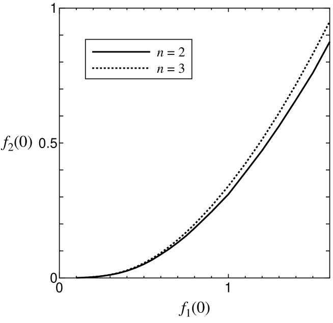
FIG. 3.: Fine-tuned value of $f_{2}(0)$ as a function of $f_{1}(0)$ in $d=4$ ($f_{0}(0)=4\pi^{2}$). The solid and dotted lines correspond to the truncations at $n=2$ and $3$, respectively.

FIG. 4.: Fine-tuned value of $f_{3}(0)$ as a function of $f_{1}(0)$ in $d=4$ ($f_{0}(0)=4\pi^{2}$).

FIG. 5.: Determination of the nonperturbative coefficient $K_{2}$ (given in (30)) in $d=4$.

FIG. 6.: Removing the nonperturbative ambiguity of $f_{2}$ on the critical surface at $f_{1}=0.1$ in $d=4$.

FIG. 7.: Fine-tuning of $f_{2}(0)$ for given values $f_{1}(0)=0.1$ and $f_{0}(0)=10.0$ in the trivial, perturbatively unrenormalizable case ($d=5$). The running time $T_{0}$ becomes maximal at $f_{2}(0)\simeq 0.0015$. $f_{1}$ and $f_{2}$ are the coupling constants for $\phi^{4}$ and $\phi^{6}$, respectively (see (15)).

FIG. 8.: The same as Fig. 6 for $d=6$. The running time $T_{0}$ becomes maximal at $f_{2}(0)\simeq 0.002$.

FIG. 9.: Fine-tuned value of $f_{2}(0)$ as a function of $f_{1}(0)$ in $d=5$ ($f_{0}(0)=1/4a$).

FIG. 10.: The same as Fig. 9 in $d=6$.

FIG. 11.: Determination of the nonperturbative coefficient $C_{2}$ (given in (82) ) in $d=5$.

FIG. 12.: The same as Fig. 11 for $d=6$, where $C_{2}$ is given in (95).

FIG. 13.: Removing the nonperturbative ambiguity of $f_{2}$ at $f_{1}(0)=0.07$on the critical surface in $d=5$.

FIG. 14.: The same as Fig. 13 for $d=6$ with $f_{1}(0)=0.15$.

REFERENCES

- [1] S. Weinerg, The Quantum Theory of Fields, Cambridge University Press, Cambridge, 1996, vol. II. Modern Applications.
- [2] S. Weinberg, Physica A96, 327 (1979); J. Gasser and H. Leutwyler, Ann. Phys. (N.Y.) 158, 142 (1984); Nucl. Phys. B250, 465 (1985).
- [3] J. Gomis and S. Weinberg, Nucl. Phys. B469, 473 (1996).
- [4] G. Ecker, Chiral perturbation theory, hep-ph/9805500; J. Bijnens, G. Colangelo and G. Ecker, Ann. Phys. 280, 100 (2000).
- [5] K. G. Wilson, Phys. Rev. B4, 3174 (1971); K. G. Wilson and J. Kogut, Phys. Rep. 12C, 75 (1974); K. G. Wilson, Rev. Mod. Phys. 47, 773 (1975).
- [6] G. ’t Hooft, The Ways of Subnuclear Physics, Proc. Int. School, Erice, Italy, 1977, ed. A. Zichichi (Plenum New York, 1978): B. Lautrup, Phys. Lett. B69, (1977) 109; G. Parisi, Phys. Lett. B76, 65 (1978); Phys. Rep. 49, 215 (1979); J. Zinn-Justin, Phys. Rep. 70, 109 (1981); M. Beneke and V. M. Braun, Renormalons and power corrections, hep-ph/0010208.
- [7] M. Lüscher and P. Weisz, Nucl. Phys. B290, 25 (1987).
- [8] S. Weinberg, Ultraviolet divergences in quantum theories of gravitation. In General Relativity, eds. S. W. Hawking and W. Israel (Cambridge Press, Cambridge,1979); J. F. Donoghue, Phys. Rev. Lett. 72, 2996 (1994); Phys. Rev. D50, 3874 (1994); Perturbative dynamics of quantum general relativity, gr-qc/9712070.
- [9] S. Carlip, Rept. Prog. Phys. 64, 885 (2001).
- [10] W. Souma, Prog. Theor. Phys. 102, 181 (1999); O. Lauscher and M. Reuter, Ultraviolet fixed point and generalized flow equation of quantum gravity., hep-th/0108040; O. Lauscher and M. Reuter, Is quantum Einstein gravity nonperturbatively renormalizable?, hep-th/0110021; M. Reuter and F. Saueressig, Renormalization group flow of quantum gravity in the Einstein-Hilbert truncation, hep-th/0110054.
- [11] P. M. Stevenson, Phys. Lett. B100, 61 (1981); Phys. Rev. D23, 2916 (1981).
- [12] F. J. Wegner and A. Houghton, Phys. Rev. A8, 401 (1973).
- [13] J. Polchinski, Nucl. Phys. B231, 269 (1984).
- [14] A. Hasenfratz and P. Hasenfratz, Nucl. Phys. B270, 685 (1986); P. Hasenfratz and J. Nger, Z. Phys. C37. 477 (1988).
- [15] C. Wetterich, Phys. Lett. B301, 90 (1993); M. Bonini, M. D’Attanasio and G. Marchesini, Nucl. Phys. B409, 441 (1993).
- [16] T. R. Morris, Int. J. Mod. Phys. B12, 1343 (1998); K-I. Aoki, Int. J. Mod. Phys. B14, 1249 (2000); J. Berges, N. Tetradis and C. Wetterich, Non-Perturbative Renormalization Group Flow in Quantum Field Theory and Statistical Physics, hep-ph/0005122.
- [17] J. F. Nicol, T. S. Chang and H. E. Stanley, Phys. Rev. Lett. 33, 540 (1974).
- [18] N. Tetradis and C. Wetterich, Nucl. Phys. B422, 541 (1994); B398 (1993) 659; J. Berges,N. Tetradis and C. Wetterich, Phys. Rev. Lett. 77, 873 (1996); Phys. Lett. B393, 387 (1997).
- [19] T. R. Morris, Phys. Lett. 329, 241 (1994); Nucl. Phys. B409, 363 (1997); T. R. Morris and M. D. Turner, Nucl. Phys. B509, 637 (1998).
- [20] K-I. Aoki, K. Morikawa, W. Souma, J-I. Sumi, and H. Terao, Prog. Theor. Phys. 95 (1996) 409; Prog. Theor. Phys. 99, 451 (1998).
- [21] M. Aizenmann, Phys. Rev. Lett. 47, 1 (1981); J. Fröhlich, Nucl. Phys. B200 [FS4], 281 (1982); C. Aragão de Carvalho, S. Carraciolo and J. Fröhlich, Nucl. Phys. B215 [FS7], 209 (1983).
- [22] M. Lüscher and P. Weisz, Nucl. Phys. B295, 65 (1988); ibid. B318, 705 (1989).
- [23] W. Zimmermann, Com. Math. Phys. 97, 211 (1985); R. Oehme and W. Zimmermann, Com. Math. Phys. 97, 569 (1985); J. Kubo, K. Sibold and W. Zimmermann, Nucl. Phys. B259, 331 (1985).
- [24] C. Becchi, On the construction of renormalized gauge theories using renormalization group techniques, hep-th/9607188.
- [25] T. Eguchi, Phys. Rev. D17, 611 (1978); I. Ya. Areféva, Ann. of Rev. 117, 393 (1979); K. Shizuya, Phys. Rev. D21, 2327 (1980); J. Zinn-Justin, Nucl. Phys. B367, 105 (1991); K-I. Kondo, S. Shuto and K. Yamawaki, Mod. Phys. Lett. A6, 3385 (1991); K-I. Kondo, M. Tanabashi and K. Yamawaki, Prog. Theor. Phys. 89, 1249 (1993); N. V. Krasnikov, Mod. Phys. Lett. A8, 797 (1993); M. Harada, Y. Kikukawa, T. Kugo and H. Nakano, Prog. Theor. Phys. 92, 1161 (1994); K-I. Kubota and H. Terao, Prog. Theor. Phys. 102, 1163 (1999).
- [26] M. Atance and J. L. Cortés, Phys. Rev. D54, 4973 (1996).
- [27] M. Atance and B. Schrempp, Infrared fixed points for rations of couplings in the chiral Lagragian, hep-ph/9912335; Infrared fixed points and fixed lines for couplings in the chiral Lagragian, hep-ph/0009069.
- [28] M. Peskin, Phys. Lett. 94B, 161 (1980).
- [29] M. Creutz, Phys. Rev. Lett. 43, 553 (1979); H. Kawai, M. Nio and Y. Okamoto, Prog. Theor. Phys. 88, 341 (1992); J. Nishimura, Mod. Phys. Lett. A11, 3049 (1996).
- [30] S. Ejiri, J. Kubo and M. Murata, Phys. Rev. D62, 105025 (2000).
- [31] H. S. Egawa, S. Horata, T. Izubuchi, N. Tsuda and T. Yukawa, Prog. Theor. Phys. 97, 539 (1997); H. S. Egawa, S. Horata and T. Yukawa, Clear evidence of a continuum theory of 4-D Euclidean simplicial quantum gravity, hep-lat/0110042.
- [32] Th. Kaluza, Sitzungsber. d. Preuss. Akad. d. Wiss., 966 (1921); O. Klein, Zeitschrift f. Phys. 37, 895 (1926).
- [33] N. Arkani-Hamed, S. Dimopoulos and G. Dvali, Phys. Lett. B 429, 263 (1998); Phys. Rev. D 59, 086004 (1999).
- [34] I. Antoniadis, N. Arkani-Hamed, S. Dimopoulos and G. Dvali, Phys. Lett. B436, 257 (1998).
- [35] L. Randall and R. Sundrum, Phys. Rev. Lett. 83, 3370 (1999); ibid. 83, 4690 (1999).
- [36] K. Dienes, E. Dudas and T. Gherghetta, Phys. Lett. B 436, 55 (1998); Nucl. Phys. B537, 47 (1999).
- [37] M. Bonini, Nucl. Phys. B421, 81 (1994); idib. B437, 163 (1995); U. Ellwanger, Phys. Lett. B335, 364 (1994); M. Reuter and C. Wetterich, Nucl. Phys. B417, 181 (1994); B427, 291 (1994); U. Ellwanger, M. Hirsch and A. Weber, Z. Phys. C69, 687 (1996); M. D’Attanasio and T. R. Morris, Phys. Lett. B378, 213 (1996); K-I. Aoki, K. Morikawa, J-I. Sumi, H. Terao and M. Tomoyose, Prog. Theor. Phys. 97, 479 (1997); ibid. 102, 1151 (1999); Phys. Rev. D61, 045008 (2000); M. Pernici, M. Raciti and F. Riva, Nucl. Phys. B520, 469 (1998); M. Pernici and M. Raciti, Nucl. Phys. B531, 560 (1998); D. F. Litim and J. M. Pawlowski, Phys. Lett. B435, 181 (1998); S. Arnone, C. Fusi and K. Yoshida, JHEP 02, 22 (1999); Y. Igarashi, K. Itho and H. So, Phys. Lett. B479, 336 (2000); T. R. Morris, JHEP 0012, 12 (2000); Nucl. Phys. B573, 97 (2000); F. Freire, D. F. Litim and J. M. Pawlowski, Phys. Lett. B495, 256 (2000); M. Simionato, Int. J. Mod. Phys. A15, 4811 (2000); S. Arnone, Y. A. Kubyshin, T. R. Morris and J. F. Tighe Gauge invariant regularization via , hep-th/0106258.
- [38] T. Kobayashi, J. Kubo, M. Mondragon and G. Zoupanos, Nucl. Phys. B550, 99 (1999); T. E. Clark and S. T. Love, Phys. Rev. D 60, 025005 (1999); J. Kubo, H. Terao and G. Zoupanos, Nucl. Phys. B574, 495 (2000).
- [39] R. J. Perry and K. G Wilson, Nucl. Phys. B403, 587 (1993).