FINITE TEMPERATURE INDUCED FERMION NUMBER

Abstract

The induced fractional fermion number at zero temperature is topological (in the sense that it is only sensitive to global asymptotic properties of the background field), and is a sharp observable (in the sense that it has vanishing rms fluctuations). In contrast, at finite temperature, it is shown to be generically nontopological, and not a sharp observable.

I Introduction

The phenomenon of induced fermion number arises due to the interaction of fermions with nontrivial topological backgrounds (e.g., solitons, vortices, monopoles, skyrmions), and has many applications ranging from polymer physics to particle physics [1, 2, 3, 4, 5]. At zero temperature, the induced fermion number is a topological quantity, and is related to the spectral asymmetry of the relevant Dirac operator, which counts the difference between the number of positive and negative energy states in the fermion spectrum. Mathematical results, such as index theorems and Levinson’s theorem, imply that the zero temperature induced fermion number is determined by the asymptotic topological properties of the background fields [6, 7, 8, 9]. This topological character of the induced fermion number is a key feature of its application in certain model field theories. At finite temperature, the situation is very different [10, 11]. In this talk I explain why at finite T the induced fermion number is generically nontopological, and is not a sharp observable.

This work has also been partly motivated by recent results that certain anomalies in $T=0$ field theory become much more subtle at nonzero $T$. For example [12], in even dim. spacetime, finite T anomalous $\pi^{0}$ decay amplitudes are T dependent even though the chiral anomaly (a topological object that is related to the anomalous $\pi^{0}$ decay amplitude at $T=0$) is independent of $T$. And, in odd dim. spacetime, the topological Chern-Simons term is the only parity-violating term induced in the $T=0$ effective action, but at finite $T$ there are infinitely many parity-violating terms [13, 14, 15].

II Induced fermion number

The induced fermion number is an expectation value of the fermion number operator, $N=\int dx\,\frac{1}{2}[\Psi^{\dagger},\Psi]$. For a given classical static background field configuration, the fermion field operator $\Psi$ can be expanded in a complete set of eigenstates of the Dirac Hamiltonian $H$. The $T=0$ fermion number, $\langle N\rangle_{0}\equiv\langle 0|N|0\rangle$, is related to the spectral asymmetry of the Dirac Hamiltonian:

$$\langle N\rangle_{0}=-\frac{1}{2}\int_{-\infty}^{\infty}dE\,\sigma(E)\,{\rm sign}(E)=-\frac{1}{2}\,({\rm spectral~{}~{}asymmetry}).$$ (1)

Here $\sigma(E)$ is the spectral function of $H$:

$$\sigma(E)=\frac{1}{\pi}\,{\cal I}m\,{\rm Tr}\left(\frac{1}{H-E-i\epsilon}\right).$$ (2)

So, $\langle N\rangle_{0}$ essentially counts the number of positive energy states minus the number of negative energy states.

At nonzero temperature $T$, the induced fermion number is a thermal expectation value

$$\langle N\rangle_{T}={{\rm Tr}\left(e^{-\beta H}\,N\right)\over{\rm Tr}\left(e^{-\beta H}\right)}=-\frac{1}{2}\int_{-\infty}^{\infty}dE\,\sigma(E)\,{\rm tanh}\left(\frac{\beta E}{2}\right)$$ (3)

where $\beta=\frac{1}{T}$. This finite T expression (3) reduces smoothly to the zero T expression (1) as $\beta\to\infty$; in fact, finite temperature provides a physically meaningful and mathematically elegant regularization of the spectral asymmetry.

Note that the spectrum of the fermions in the static background has nothing to do with the temperature. All information about the fermion spectrum is encoded in the spectral function. Thus, if one knows $\sigma(E)$, one immediately has integral representations for both $\langle N\rangle_{0}$ and $\langle N\rangle_{T}$. In fact, one only needs to know the odd part of $\sigma(E)$, as is clear from (1) and (3). It is convenient to use the explicit form (2) of the spectral function to write (3) as a contour integral involving the resolvent of the Dirac Hamiltonian

$$\langle N\rangle_{T}=-\frac{1}{2}\int_{\cal C}\frac{dz}{2\pi i}\,{\rm Tr}\left(\frac{1}{H-z}\right)\,{\rm tanh}\left(\frac{\beta z}{2}\right)$$ (4)

where ${\cal C}$ is the contour $(-\infty+i\epsilon,+\infty+i\epsilon)$ and $(+\infty-i\epsilon,-\infty-i\epsilon)$ in the complex energy plane. Thus the resolvent is the key to the computation.

III Two 1+1 dimensional examples

Before going to the general case, it is instructive to consider two important cases in 1+1 dim field theory. These two examples are very similar at T=0, but turn out to be very different for $T>0$. Consider an abelian model of fermions interacting via scalar and pseudoscalar couplings to two (classical, static) bosonic fields $\phi_{1}$ and $\phi_{2}$:

$${\cal L}=i\,\bar{\psi}\partial\hskip-5.0pt/\,\psi-\bar{\psi}\left(\phi_{1}+i\,\gamma_{5}\,\phi_{2}\right)\psi$$ (5)

We distinguish between two different cases:

(a) kink case [1]: $\phi_{1}=m$ is constant, but $\phi_{2}(x)$ has a kink-like shape (for example $\phi_{2}(x)={\rm tanh}(x)$), with $\phi_{2}(\pm\infty)=\pm\hat{\phi_{2}}$.

(b) sigma-model case [2]: $\phi_{1}(x)$ and $\phi_{2}(x)$ are constrained to the “chiral circle”: $\phi_{1}^{2}+\phi_{2}^{2}=m^{2}.$

The kink case (a) is relevant to the polymer physics applications, while the sigma-model case (b) is a low-dimensional analogue of sigma models used in 3+1 dim. particle physics models [4].

In each case, we define the angular field

$$\theta(x)\equiv{\rm arctan}\,\left[\phi_{2}(x)/\phi_{1}(x)\right]$$ (6)

In the sigma model case (b), the angular field $\theta(x)$ has the interpretation of a local chiral angle, and is chosen to have a kink-like shape, with asymptotic values $\theta(\pm\infty)\equiv\pm\hat{\theta}$. Note that in the kink case (a), the angular field $\theta(x)={\rm arctan}[\phi_{2}(x)/m]$ also has a kink-like shape.

For both the kink case and the sigma-model case, at zero T, the induced fermion number is

$$\langle N\rangle_{0}=\frac{1}{2\pi}\int dx\,\theta^{\prime}(x)=\frac{\hat{\theta}}{\pi}$$ (7)

which is topological in the sense that it only depends on the asymptotic values of $\theta(x)$, not on its detailed shape. In the kink case, this calculation is easy because the even part of the corresponding Dirac resolvent is known exactly [16]

$$\left[{\rm Tr}\left(\frac{1}{H-z}\right)\right]_{\rm e}={-m\hat{\phi}_{2}\over(m^{2}-z^{2})\,\sqrt{m^{2}+\hat{\phi}_{2}^{2}-z^{2}}}$$ (8)

But in the sigma-model case the resolvent is not known exactly, and one must resort to an approximation such as the derivative expansion. Nevertheless, both cases lead to the same result (7).

At finite T, the kink case is also easy because we know the relevant part of the resolvent exactly [17]. Inserting (8) into the contour integral expression (4) one finds

$$\langle N\rangle_{T}^{\rm kink}=\sum_{n=0}^{\infty}{\frac{2}{\pi}\,(\frac{m\beta}{\pi})^{2}{\rm sin}\hat{\theta}\over((2n+1)^{2}+(\frac{m\beta}{\pi})^{2})\sqrt{(2n+1)^{2}{\rm cos}^{2}\hat{\theta}+(\frac{m\beta}{\pi})^{2}}}$$ (9)

Note that $\langle N\rangle_{T}^{\rm kink}$ is temperature dependent, but it is still topological in the sense that it only depends on the background field through its asymptotic value $\hat{\theta}={\rm arctan}[\hat{\phi_{2}}/m]$. Also, even though the expression (9) looks complicated, it smoothly reduces to (7) as $T\to 0$. It is also interesting that the angular nature of $\hat{\theta}$ is more obvious at finite T than at zero T.

At finite T, the sigma-model case is much more complicated, because there is no simple closed formula for the relevant part of the resolvent. In [10] the derivative expansion was used, and it was shown that for $T\ll m$ the derivative expansion can be resummed to all orders, leading to the following simple expression

$$\langle N\rangle_{T}^{\rm sigma}=\langle N\rangle_{0}^{\rm sigma}-\sqrt{\frac{2m}{\beta\pi}}\int dxe^{-m\beta}\,\sinh\left(\frac{\beta\theta^{\prime}}{2}\right)+\dots$$ (10)

The correction term is temperature dependent and nontopological, as it is sensitive not just to the asymptotic values of $\theta(x)$, but also to the details of the shape of $\theta(x)$. This nontopological term has a simple physical interpretation as follows [10]. For the sigma model case we can write the interaction term in (5) as $m\bar{\psi}\left(\cos\theta+i\gamma_{5}\sin\theta\right)\psi=m\bar{\psi}\,e^{i\gamma_{5}\theta}\psi$. Then make the local chiral rotation $\psi=e^{-i\gamma_{5}\theta/2}\,\tilde{\psi}$ to obtain

$${\cal L}=i\bar{\tilde{\psi}}\partial\hskip-5.0pt/\tilde{\psi}-m\bar{\tilde{\psi}}\tilde{\psi}+\bar{\tilde{\psi}}\,\gamma^{0}\,\frac{\theta^{\prime}}{2}\,\tilde{\psi}$$ (11)

which describes a fermion of mass $m$ in an inhomogeneous electric field $E(x)=-\frac{1}{2}\theta^{\prime\prime}(x)$. In this language the zero T induced fermion number (7) can be understood as the vacuum polarization, due to the inhomogeneous electric field background, of virtual vacuum $e^{+}e^{-}$ dipoles. This effect is independent of the temperature as the virtual vacuum dipoles do not live long enough to thermalize. However, at finite T there is another effect of the background electric field. The real particles and antiparticles respond to this electric field in a way that can be described by linear response theory. In the derivative expansion limit, where $\theta^{\prime}\ll m$, the leading effect of the electric field background can be represented as a local chemical potential $\mu(x)=-\frac{1}{2}\theta^{\prime}(x)$. With local Fermi distributions

$$f_{\pm}(x,k)={1\over e^{\beta(\sqrt{k^{2}+m^{2}}\,\mp\mu(x))}+1}$$ (12)

the linear response charge density is $\rho(x)=\int\frac{dk}{2\pi}\,f(x,k)$, where $f=f_{+}-f_{-}$. For $T\ll m$,

$$\rho(x)\sim-\sqrt{\frac{2mT}{\pi}}\,e^{-m/T}\,\sinh\left(\frac{\theta^{\prime}}{2T}\right)$$ (13)

in perfect agreement with the non-topological term in (10).

So, while at zero T, the kink and sigma-model cases each have induced fermion number given by the same expression (7), at nonzero T they have very different induced fermion number, given by (9) and (10) respectively. In each case $\langle N\rangle_{T}$ is temperature dependent, but in the kink case it is topological, while in the sigma-model case it is nontopological. The physical reason for this difference is explained in the next section.

IV Topological versus Nontopological

The straightforward mathematical reason why $\langle N\rangle_{T}$ is topological for the kink case is that the odd part of the spectral function is itself topological, as shown by the Callias result (8). But a much more physical understanding can be obtained by considering the symmetries of the fermionic spectrum [11]. And this perspective generalizes immediately to higher dimensional models.

Begin with the simple trigonometric identity, $\tanh(\frac{\beta E}{2})=1-2n(E)$, where $n(E)=1/(e^{\beta E}+1)$ is the Fermi-Dirac distribution function. Then the finite T fermion number (3) separates as

$$\langle N\rangle=\langle N\rangle_{0}+\int_{-\infty}^{\infty}dE\,\sigma(E)\,{\rm sgn}(E)\,n(|E|)$$ (14)

The first term is just the zero temperature contribution, which can be expressed in terms of the spectral asymmetry, and is known to be topological. But the second term is highly sensitive to the details of the spectrum, because of the presence of the Fermi weighting factor $n(|E|)$. Thus, the only way this term can be topological is if the odd part of $\sigma(E)$ is itself topological. In terms of the spectrum, this can only happen if the spectrum is symmetric under $E\to-E$. Remarkably, this does sometimes happen, but only for extremely special backgrounds. One example of such a special background is the one-dim kink background discussed in the previous section. Indeed, for any kink background (with $\hat{\theta}$ positive), the spectrum of the Dirac Hamiltonian always has the form shown in Fig. 1.

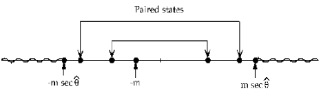
FIG. 1.: The general structure of the Dirac spectrum for a kink background.

There are continuum states for $|E|>\sqrt{m^{2}+\hat{\phi}_{2}^{2}}=m\,{\rm sec}\,\hat{\theta}$. In addition, there is always a bound state at $E=-{\rm sign}(\hat{\theta})\,m$. There may or may not be additional bound states with $m<|E|<m\,{\rm sec}\,\hat{\theta}$. But if these additional bound states are present, they necessarily occur in $\pm E$ pairs, because of the quantum mechanical SUSY of the Dirac Hamiltonian in the kink case [4]. Thus, the contributions of these paired bound states to the integral in (14) cancel in pairs, while the unpaired bound state at $E=-{\rm sign}(\hat{\theta})\,m$ leads to a contribution $-{\rm sign}(\hat{\theta})\,n(m)$. The quantum mechanical SUSY of the Dirac Hamiltonian is likewise the key to the exact Callias index theorem result [16] for the odd part of the spectral function [which is equivalent to knowing the even part of the resolvent in (8)]. This means that the remaining integral over the continuum states can be expressed as an integral of the odd part of the spectral function, weighted by the Fermi factor $n(E)$, over the positive continuum beginning at the threshold energy $m{\rm sec}\hat{\theta}$. Putting all this together, we obtain

$$\langle N\rangle_{T}^{\rm kink}=\langle N\rangle_{0}^{\rm kink}-n(m)+\int_{m\,{\rm sec}\,\hat{\theta}}^{\infty}\frac{dE}{\pi}\,\frac{2m^{2}\tan\hat{\theta}\,n(E)}{(E^{2}-m^{2})\sqrt{E^{2}-m^{2}{\rm sec}^{2}\hat{\theta}}}$$ (15)

One can check that this is, in fact, the Sommerfeld-Watson transform of the summation expression found before in (9).

FIG. 2.: The structure of the Dirac spectrum for a sigma model background.

On the other hand, for the sigma-model case the fermion spectrum has no obvious symmetry. In this case, the Dirac spectrum has the form shown in Fig. 2. The only general thing we can say is that the continuum thresholds are at $E=\pm m$. There may or may not be one or more bound states for $|E|<m$. The existence of (and the precise location of) bound states is highly sensitive to the actual shape of the $\theta(x)$. As there is no special symmetry in the spectrum, there is nothing general that can be said about the odd part of the spectral function. Nevertheless, the first term in (14), which is $\langle N\rangle_{0}$, yields a topological result since the integral can be written, using Levinson’s theorem, in terms of the phase shift at infinity, which is topological [6, 7, 9]. This application of Levinson’s theorem doesn’t work for the T dependent second term in (14) because of the Fermi factor. This is another way to understand why the finite temperature induced fermion number is generically nontopological.

These arguments based on the symmetry of the fermion spectrum (in the given background) clearly generalize to any dimension of spacetime. So, we conclude that the generic situation is that the finite T induced fermion number is non-topological; but, if the background is such that the fermion spectrum is highly symmetric, then the induced fermion number may be topological even though it is temperature dependent.

V Thermal fluctuations of fermion number

Fluctuations in the induced fermion number can be analyzed in an analogous manner [11]:

$$(\Delta N)^{2}\equiv\langle N^{2}\rangle-\langle N\rangle^{2}=\frac{1}{4}\int_{-\infty}^{\infty}dE\,\sigma(E)\,{\rm sech}^{2}\left(\frac{\beta E}{2}\right)$$ (16)

The trigonometric identity, $\frac{1}{4}{\rm sech}^{2}(\frac{\beta E}{2})=n(E)(1-n(E))$, re-expresses this as

$$(\Delta N)^{2}=\int_{-\infty}^{\infty}dE\,\sigma(E)\,n(E)\left(1-n(E)\right)$$ (17)

which is simply a sum over the fermion spectrum of $n(1-n)$, as it should be for the thermal occupation of independent single-particle states [20]. From (17) it is clear that the fluctuations are always non-topological, as they are sensitive to the details of the fermion spectrum. Another way to see this is to note that the expressions (16,17) require knowledge of the even part of the spectral function, which is not accessible to an index theorem. So the fluctuations must typically be calculated approximately; however, for a special class of kink backgrounds, $\phi_{2}(x)=\hat{\phi}\tanh(\hat{\phi}x/j)$, where $j$ is an integer, it is possible to compute $(\Delta N)^{2}$ exactly, and one sees the explicit (nontopological) dependence on the scale factor $j$ [11].

These expressions also make it clear why the fluctuations vanish at zero T, because the ${\rm sech}^{2}(\beta E/2)$ factors vanish exponentially fast as $T\to 0$. Thus, the induced fermion number is a sharp observable at $T=0$, in agreement with previous results [18], but at nonzero T it is not a sharp observable, simply because the thermal expectation value mixes states other just the ground state. Another example of non-sharp fractional fermion number (but not in the context of temperature dependence) has been discussed recently in the context of liquid helium bubbles [19].

VI Conclusions

To conclude, the finite temperature induced fermion number $\langle N\rangle_{T}$ is generically nontopological, and is not a sharp observable. The induced fermion number naturally splits into a topological temperature-independent piece that represents the effect of vacuum polarization on the Dirac sea, and a nontopological temperature-dependent piece that represents the thermal population of the available states in the fermion spectrum, weighted with the appropriate Fermi-Dirac factors. As the temperature approaches zero, the nontopological terms vanish exponentially fast, and we regain smoothly the familiar topological results at zero temperature. But at nonzero temperature, the nontopological contribution is more sensitive to the details of the spectrum, and so is generically nontopological. This argument applies in any dimension.

Consider, for example, for a chiral $SU(2)$ sigma model with a Skyrme background in 3+1 dim.,

$${\cal L}_{\rm int} = m\bar{\psi}\left(\pi_{0}+i\gamma_{5}\vec{\pi}\cdot\vec{\tau}\right)\psi$$ (18)

$$= m\bar{\psi}\left(\frac{1}{2}(g+g^{\dagger})+\frac{1}{2}(g-g^{\dagger})\gamma_{5}\right)\psi$$ (19)

where $\pi_{0}^{2}+\vec{\pi}^{2}=1$ and $\pi_{0}+i\vec{\pi}\cdot\vec{\tau}=g$, which is the analogue of the 1+1 dim. sigma-model case analyzed in this paper. From numerical work [21], the Dirac energy spectrum of the fermions is not symmetric, and the energy of a possible bound state (and indeed the number of bound states) is highly sensitive to the details of the shape of the radial hedgehog field. This shows that in this case the finite temperature induced fermion number is nontopological. Thus, for a (large) Skyrme background in 3+1 dim., the finite temperature fermion number is not simply the (topological) winding number of the Skyrme field, but a much more complicated nontopological object.

Acknowledgement: This talk is based on work done in collaboration with Ian Aitchison and Kumar Rao. I also thank the US DOE for support.

REFERENCES

- [1] R. Jackiw and C. Rebbi, Phys. Rev. D 13 (1976) 3398.
- [2] J. Goldstone and F. Wilczek, Phys. Rev. Lett. 47 (1981) 986.
- [3] J. Goldstone and R. L. Jaffe, Phys. Rev. Lett. 51 (1983) 1518.
- [4] A. Niemi and G. Semenoff, Phys. Rep. 135 (1986) 99.
- [5] A. J. Heeger, S. Kivelson, J. R. Schrieffer and W. P. Su, Rev. Mod. Phys. 60 (1988) 781.
- [6] R. Blankenbecler and D. Boyanovsky, Phys. Rev. D 31 (1985) 2089.
- [7] M. Stone, Phys. Rev. B 31 (1985) 6112.
- [8] A. P. Polychronakos, Phys. Rev. D 35 (1987) 1417.
- [9] E. Farhi, N. Graham, R. L. Jaffe and H. Weigel, Nucl. Phys. B595 (2001) 536.
- [10] I. J. R. Aitchison and G. V. Dunne, Phys. Rev. Lett. 86 (2001) 1690.
- [11] G. V. Dunne and K. Rao, Phys. Rev. D 64 (2001) 025003.
- [12] R. Pisarski, T.L. Trueman and M. Tytgat, Prog. Theor. Phys. Suppl. 131 (1998) 427.
- [13] G. Dunne, K. Lee and C. Lu, Phys. Rev. Lett. 78 (1997) 3434; G. Dunne, “Aspects of Chern-Simons Theories”, Les Houches 1998, Topological Aspects of Low Dimensional Systems, A. Comtet et al (Eds), (Springer, 1999).
- [14] S. Deser, L. Griguolo and D. Seminara, Phys. Rev. Lett. 79 (1997) 1976; Phys. Rev. D 57 (1998) 7444; Commun. Math. Phys. 197 (1998) 443.
- [15] C. Fosco, G. Rossini and F. Schaposnik, Phys. Rev. Lett. 79 (1997) 1980, (Erratum), ibid 79 (1997) 4296; Phys. Rev. D 56 (1997) 6547; Phys. Rev. D 59 (1999) 085012.
- [16] C. Callias, Comm. Math. Phys. 62 (1978) 213.
- [17] A. Niemi and G. Semenoff, Phys. Lett. B 135 (1984) 121.
- [18] S. Kivelson and J. R. Schrieffer, Phys. Rev. B 25 (1982) 6447; R. Jackiw, A. Kerman, I. Klebanov and G. Semenoff, Nucl. Phys. B225 (1983) 233.
- [19] R. Jackiw, C. Rebbi and J. R. Schrieffer, “Fractional Electrons in Liquid Helium?”, cond-mat/0012370.
- [20] R. Pathria, Statistical Mechanics, (Pergamon Press, Oxford, 1972).
- [21] S. Kahana and G. Ripka, Nucl. Phys. A429 (1984) 462; G. Ripka, Quarks bound by chiral fields, (Clarendon Press, Oxford, 1997).