HU-EP 01/46,

hep-th/0110201

String–String triality for ${\bf d=4}$, ${\bf Z_{2}}$ orbifolds^†
Andrea Gregori
Humboldt-Universität, Institut für Physik
D-10115 Berlin, Germany

Abstract
We investigate the perturbative and non-perturbative correspondence of a class of four dimensional dual string constructions with ${\cal N}=4$ and ${\cal N}=2$ supersymmetry, obtained as $Z_{2}$ or $Z_{2}\times Z_{2}$ orbifolds of the type II, heterotic and type I string. In particular, we discuss the heterotic and type I dual of all the symmetric $Z_{2}\times Z_{2}$ orbifolds of the type II string, classified in Ref. [1].

 ^†  Research supported by the “Marie Curie” fellowship HPMF-CT-1999-00396.
¹e-mail: agregori@physik.hu-berlin.de

1 Introduction

After the appearance of Refs. [2] and [3], the duality between the heterotic, the type II and the type I string in less than six dimensions, and notably in four dimensions, has been one of the major subjects of investigation some years ago. In some specific cases, tests of this duality have been provided [4, 5], and, once understood some general “rules” for the identification of string duals [6], started a “systematic” investigation of certain non-perturbative properties of string constructions, in particular of the heterotic string [7, 8, 9, 10, 11, 12] . However, most of these analyses, although applied to string theory, as a matter of fact rely more on supergravity, field theory and the properties of supersymmetry or even of algebraic geometry, than on real properties of the string theory as such, deeply distinguished from any of the legitimate ingredients of its effective descriptions. In fact, the relation between string theory, namely a theory expected to be “the” quantum theory of gravity and gauge interactions, and its representations in terms of supergravity or field theory, allowed in certain limits, is rather subtle. As a matter of fact, many tests of string–string duality are actually no much more than consistency tests of the duality among the underlying effective supergravities. What makes a hard task to really test string–string dualities in a string framework, besides the lack of knowledge of a non-perturbative definition of the theory, is that, already at the perturbative level, the partition function at a generic point of the perturbative moduli space is not known. We nevertheless consider such tests the only way of getting, when possible, reliable informations, minimizing thereby the possibility of falling into the trap of “tautologies”, a risk always present when investigating string dualities through the projection onto a “sub-sector” of the theory, such as supergravity or field theory.

For similar reasons, we also still consider direct string constructions something based on a more solid ground than string vacua obtained through the reduction of higher dimensional theories such as, for instance, F-theory. The only way of testing the reliability of these vacua is through the comparison with string theory; once these conditions have been taken into account, these vacua turn out to provide no more informations than what one can already obtain from the string theory itself.

In this work we therefore investigate string–string duality in four dimensions by taking a “conservative” attitude, going back to “simple” examples for which we have direct, explicit string constructions. Our aim is to provide an analysis free of the prejudices that may be induced by supergravity/field-theory considerations, not always appropriate to the analysis of superstrings. String–string duality is in fact more fundamental than supergravity dualities, and has its origin in the expected equivalence of the various “regularization” procedures of the ultraviolet divergences, corresponding to the different “types” of strings. The duality between string constructions therefore does not necessarily imply a duality of the corresponding effective supergravity theories . Taking this into account, we decided to base our investigation on direct string computations, extracting as much information as possible from the comparison of dual string constructions, and avoiding any non-necessary assumption. In practice, we reconsider the heterotic/type II/type I string–string duality in the case of ${\cal N}=4,2$ supersymmetry in four dimensions, for $Z_{2}$ orbifold constructions . As is known, in less than ten dimensions it may happen that not all the massless degrees of freedom appear explicitly in the perturbative spectrum of a certain string construction, even at weak coupling. This is the case of certain gauge states for the type II string, in which the states charged under the RR fields don’t have a representation in terms of vertex operators, and do not appear in the perturbative spectrum; or the case of massless states appearing when heterotic instantons shrink to zero size. This makes the identification of string dual pairs something that has to be handled with care, starting from the very choice of the criteria that allow to identify such pairs: we in fact cannot expect to always have a perturbative–perturbative duality, with an exact correspondence of the two perturbative effective theories. This leaves open an apparent arbitrariness in the identification of dual pairs. For instance, the fact that, although existing, gauge charged states never appear on the type II side, implies that a wide choice of gauge configurations on the heterotic side may correspond to the same type II construction. The case of heterotic “small instantons” is particularly delicate: such states may appear in fact for special values of the moduli in the hypermultiplets, and the $T^{4}\big{/}Z_{2}$ orbifold point of the K3 is precisely a special point in the hypermultiplets space. We should therefore not be too surprised to find that, in some cases, precisely at this point the massless spectrum possesses a non-perturbative extension. Although deceiving this may look, it has not to be taken as a total impossibility of determining dual pairs. The point of view we took is that one should not expect a naive coincidence of massless spectra, often forbidden by accidental technical facts, such as the impossibility of constructing certain vertex operators, nor an automatic coincidence of the moduli spaces of the supergravity theories associated to the perturbative spectrum, or, even worse, a “fiber-wise” correspondence of the geometric spaces on which the various ten dimensional strings are compactified: a geometric correspondence doesn’t imply in general a correspondence of the quantum moduli spaces . Rather, our general guidelines have been:
i) to first identify the general criteria of why certain states may or may not appear in the perturbative spectrum of a certain string construction, and only after the identification of which subsets of the massless spectrum of the string theory may appear in the specific, heterotic or type II, or type I construction, to proceed to the comparison of the spectra of different string constructions.
ii) to rely on the comparison of quantities explicitly, independently computed on the various string constructions, avoiding therefore any use of “index” theorems, or conjectures based on the properties of supersymmetry. We did not want in fact to exclude a priori the possibility that exact supersymmetry may be only an approximation.
iii) to require compatibility with the perturbative properties (spectrum, symmetries) of the various string realizations, in the appropriate weak coupling limits.

Even by proceeding in this way, a certain amount of arbitrariness and assumptions has been necessary. This is somehow unavoidable; otherwise, any duality test would be “tautological”, and string-string duality would loose its major interest, namely the predictive power. Nevertheless, we find that the criteria we used are quite reasonable and, as it will be clear from the analysis of the various cases, very restrictive. Although we cannot “prove” the dualities, it is encouraging that the picture we find is extremely consistent, and allows to clarify several aspects of string theory.

The paper is organized as follows:

After a brief introduction to the subject in section 2, our analysis begins with a review of string–string duality for ${\cal N}=4$ supersymmetry, in section 3. This section serves us to clarify certain points, that will reappear in the subsequent sections, and to start “setting the rules” of the analysis. One of the quantities that will guide the following investigation is the mass formula of the string states that are “lifted” by freely acting projections. In such cases, the masses of the states acquire a dependence on the string moduli. Depending on whether these moduli are perturbative or non-perturbative, and whether the masses are suppressed or blow up in the perturbative limit, these states may or may not appear in a certain string construction. This is therefore an essential key in order to properly identify the string duals: in particular, it was the guideline for a new orientifold construction, presented in section 3.2, in which the world-sheet parity projection acts freely.

We pass then, in section 4, to the analysis of ${\cal N}=2$ orbifolds, freely and non-freely acting. In the first case, the massless spectrum is just a projection of the dimensionally reduced supergravity spectrum of ten dimensions. In the second case the spectrum contains additional states, associated to the orbifold fixed points, and originating from the twisted sectors. On the heterotic side, these states are hypermultiplets, while on the type IIA and type I side contain in general also new vector multiplets. On the type I side, the “twisted” sector appears in the form of a D5 branes sector. The case of non-freely acting orbifolds proves to be the most interesting one: precisely in this case, on the type IIA side the compact space cannot be interpreted as a limit of a K3 fibration. Therefore, there cannot be a “perturbative” correspondence with the heterotic string: the type IIA spectrum contains in fact states that are of non-perturbative origin from the heterotic point of view. This however by no means forbids a test of string–string duality. These states are in fact of the “small instantons” type; they are therefore present even in the heterotic weak coupling limit, they interact with the “perturbative” ones, and indirectly contribute to the renormalization of quantities that we can compute in string perturbation. Quite remarkably, it is possible to define amplitudes, built on $R^{2}$ and $F^{2}$ terms, that allow to unambiguously test string–string duality through a comparison of direct computations performed on the type II, heterotic and type I sides [1, 14, 15, 16]. As we will see, when the dual constructions are properly identified, there is an astonishing correspondence of these amplitudes: the contributions of the moduli related by duality appear through the same function, with a coincidence even in its normalization.

The analysis of duality in the case of freely acting, or semi-freely acting, orbifolds, makes on the other hand use, as we said, of the informations provided by the moduli-dependence of the mass of certain states. Particularly interesting are the cases of those semi-freely acting orbifolds in which the free part of the orbifold action is visible only on the type II, or type I side, because it involves an action on the modulus dual to the heterotic dilaton. From the heterotic point of view, they appear therefore as ordinary, non-freely acting orbifolds, from which they are distinguished only by the non-perturbative behavior, at non-zero string coupling. Again, the (heterotic) perturbative physics is not however completely blind to these phenomena, and still the heterotic dual can be unambiguously identified. From string–string duality, we then learn that, from the heterotic point of view, in these constructions the gauge group is of entirely non-perturbative origin.

The identification of the mechanism of rank reduction, in all the dual string constructions, allows then us to complete the analysis of the ${\cal N}_{4}=2$, $Z_{2}$ orbifolds, and ultimately provide the heterotic and type I dual for all the $Z_{2}\times Z_{2}$ type II orbifolds of Ref. [1], i.e. of all the $Z_{2}\times Z_{2}$ orbifolds of the type II string in which each $Z_{2}$ projection acts as a left–right symmetric twist of four coordinates.

All the string vacua considered in section 4 present gauge groups with vanishing (one loop) gauge beta-function. In ${\cal N}_{4}=2$ string theory a non-vanishing gauge beta-function always introduces in the expression of the effective coupling other moduli, among which there are those parameterizing the coupling constant of “hidden” gauge sectors, of the “small instantons” type. The appearance of these couplings raises a puzzle of ${\cal N}_{4}=2$ string theory. On one hand, we expect in fact the string corrections to the gauge coupling, as it is sensitive to the couplings, to be also sensitive to the mass of the states of these hidden sectors, in such a way that, as they become massive and decouple, their contribution to the correction vanishes; on the other hand, the masses of these states depend on the moduli in the hypermultiplets, and these are forbidden by ${\cal N}_{4}=2$ supersymmetry to enter in the expressions of the corrections to the gauge couplings. In section 5 we propose a physical interpretation that allows to solve this paradox. By considering the peculiar way the couplings of the hidden sectors enter into the gauge corrections, we argue that, as soon as there is a non-vanishing gauge beta-function, the visible sector interacts with the hidden sector, which is now in a phase of strong coupling. Supersymmetry is therefore broken because of gaugino condensation in the hidden sector. The breaking of supersymmetry is non-perturbative from the point of view of the visible sector, that therefore appears, in a perturbative construction, as an expansion around an ${\cal N}_{4}=2$ vacuum. However, the fact that supersymmetry is broken forbids the use of “index” theorems in order to promote the string corrections, as explicitly computed for instance in the heterotic or type I string at the orbifold point, to a result valid at other points in the moduli of the compact space. According to this interpretation, results such as those of Refs. [17, 18, 19, 20] would be universally valid only in the case of vanishing gauge beta-functions.

The breaking of supersymmetry in theories with non-vanishing gauge beta-functions is peculiar of string theory, and does not have a counterpart in field theory, in which a beta-function does not imply an interaction with “hidden” sectors.

2 Heterotic/type IIA/type I duality

In this section we review some old topics about string-string duality between the heterotic, the type IIA and the type I string in (six and) four dimensions. Throughout the paper, we will use the convention to indicate the number ${\cal N}$ of space-time supersymmetries in $d$ dimensions as ${\cal N}_{d}$.

2.1 Heterotic/type IIA duality

We start by considering the duality between the heterotic and the type IIA string. We consider here general properties, valid for compactifications on spaces more general than the $Z_{2}$ orbifolds, to which we will restrict from section 3.

2.1.1 ${\cal N}_{6}=2$ and ${\cal N}_{4}=4$

The heterotic string toroidally compactified to six dimensions has been conjectured to be dual to the type IIA string compactified on a K3 [2, 21, 22], through an inversion of coupling. When further compactified on a two-torus, the two four-dimensional theories are then mapped the one into the other by exchanging a modulus of the gravity manifold (the dilaton–axion field $S$) with a modulus, $T$, of the vector manifold [21, 22]. This conjecture of duality is based on the comparison of the low energy effective actions of the two theories, and is supported by several tests, essentially relying on properties typical of the extended supersymmetry [4, 5, 6]. The reason why tests based on extended supersymmetry properties are very reliable is that in the ${\cal N}_{6}=2\big{/}{\cal N}_{4}=4$ case all the non-perturbative phenomena are suppressed in the weak coupling limit. The field content of the theory, that determines the corresponding effective supergravity, is easily accessible via a perturbative analysis on the heterotic side, and can be compared with what one derives from a geometric analysis on the type IIA side, “simple” because of the uniqueness of the K3 surface. Once identified the underlying supergravity/super Yang–Mills theory, one then simply uses the properties of extended supersymmetry.

2.1.2 ${\cal N}_{4}=2$

More complicated is the case in which supersymmetry is reduced by half (in this case, the heterotic/type IIA duality exists only in four dimensions). On the heterotic side, such a reduction of supersymmetry is obtained, in the case of constructions that admit a geometric interpretation, by compactifying six coordinates on $T^{2}\times K3$ and choosing an appropriate gauge bundle. The K3 surface admits several orbifold limits. In these cases, the orbifold operation in four of these six coordinates can be coupled to translations acting on $T^{2}$. An analysis based on the properties of the effective ${\cal N}=2$ supergravity theory, as derived from the spectrum of the heterotic string, indicates that the type IIA dual of such a heterotic construction has to be found among the type IIA vacua obtained by compactification on a Calabi–Yau manifold which is also a K3 fibration [6]. This observation is based on the analysis of the prepotential, a holomorphic function of the moduli of the vector manifold, that encodes the informations about the couplings involving the vector multiplets. The prepotential corresponding to the effective theory built on the perturbative massless fields of the heterotic compactification reads:

$${\cal F}=S(TU-\sum_{i}C^{i}C^{i})+{\rm F}_{0}(T,U,C^{i})+{\rm F}_{\rm n.p.}({\rm e}^{-S},T,U,C^{i})\,,$$ (2.1)

where $T$, $U$ are the moduli associated respectively to the Kähler class and the complex structure of the two-torus, while $C^{i}$ are associated to the scalars in the vector multiplets originating from the currents. The term ${\rm F}_{0}(T,U,C^{i})$ contains terms of the type $c_{abc}y^{a}y^{b}y^{c}$, cubic in these fields. The heterotic dilaton–axion field $S$ corresponds to the complex modulus associated to the volume of the base of the fibration.

For particular configurations of the K3 space, the heterotic string contains additional vector multiplets, entirely non-perturbative. These states appear when instantons shrink to zero size. This phenomenon depends on the particular configuration of the K3, i.e. on the moduli in the hypermultiplets, and, although of non-perturbative origin, it cannot be eliminated by going to the very weak coupling limit: this effect in fact is not exponentially suppressed by the field $S$. According to the analysis of Ref. [6], from the dual point of view of the type IIA string compactified on a K3 fibration, these new states appear when the fiber degenerates.

2.2 Heterotic/type I duality in four dimensions

From the comparison of the effective actions, one can see that the duality between the heterotic and the type I string in four dimensions, in the case of ${\cal N}=4$ supersymmetry, is “perturbative-perturbative”, the heterotic modulus $S$ being mapped into an analogous modulus of type I, parameterizing the coupling of the D9-branes . Duality with ${\cal N}=4$ supersymmetry means that the two theories are indeed the same theory. However, it is not always easy to identify the duality map between heterotic and type I string. When supersymmetry is reduced to ${\cal N}=2$, in the type I string there can be additional D-branes sectors, e.g. D5-branes, and certain states, perturbative on the type I side, may map to non-perturbative ones of the heterotic string. On the other hand, it happens also that certain perturbative moduli of the heterotic theory map into non-perturbative ones on the type I side. This implies that a perturbative phase of the heterotic string may not correspond to a perturbative phase of the type I string. An important aspect of the type I string, that has to be taken into account when comparing with the heterotic string, is that there is never mixing between the couplings of two different sectors that appear explicitly, as D-branes sectors, on the type I side. For instance, in the $U(16)\times U(16)$ model of Ref. [23], there are hypermultiplets charged under both the $U(16)$’s. From a field theory point of view, we would then expect a non-vanishing one-loop renormalization of the effective gauge coupling of the D9-brane sector depending on the coupling of the D5-branes. In four dimensions, the first is parameterized by a field $S$, the second by a field $S^{\prime}$, and we would expect a correction of the type :

$${1\over g^{2}_{9}}_{\rm(4-dim)}\,\equiv\,S_{2}\;\to\;\approx\,S_{2}\,+\,\beta\,S^{\prime\,-1}_{2}\,.$$ (2.2)

However, on the type I side this correction is always non-perturbative, and never appears explicitly. Notice that such a renormalization would exist even when the D5-branes sector is made massive by some Higgs-mechanism. Neither the D9-branes nor the D5-branes sector of a type I model with such a structure can therefore be dual to the heterotic currents: one of the two couplings would in fact correspond to a perturbative modulus of the heterotic string, and its contribution should appear explicitly at the one-loop, but with the opposite power (see section 4.1.2 for more details). Therefore, even though at the ${\cal N}_{4}=4$ level the heterotic/type I duality implies the identification of the D9-branes sector with the currents on the heterotic side, when supersymmetry is reduced to ${\cal N}_{4}=2$ it is not always true that the D9-branes sector of the type I string maps into the sector corresponding to the perturbative currents of the heterotic string. As we will see, the relation between heterotic and type I constructions may be rather non-trivial; in certain cases, all the D-branes states correspond to non-perturbative states on the heterotic side. Our aim in the following is precisely to understand what is the recipe for the identification of this map, for the moduli in the vector multiplets, at least in the simple case of $Z_{2}$ orbifolds.

In what follows, we will therefore restrict our analysis to the case of $Z_{2}$, ${\cal N}_{4}=4$ and $Z_{2}\times Z_{2}$, ${\cal N}_{4}=2$ orbifold constructions of the type II string. We then provide the explicit construction of the heterotic and type I duals, for which we also write the partition function. This will allow us to test our conjectures through direct string computations, thereby going beyond supergravity considerations.

3 ${\bf Z_{2}}$ orbifolds: ${\bf{\cal N}_{4}\boldsymbol{=}4}$

In this section we discuss how string-string duality works in certain examples for which the theory can be realized as a $Z_{2}$ orbifold of the type IIA string. From the heterotic (and type I) point of view, these theories can be divided into two classes: those with unbroken and those with broken $SL(2,Z)$ duality of the dilaton–axion field $S$.

3.1 unbroken S-duality

We start by reconsidering the case of ${\cal N}=4$ supersymmetry in four dimensions. The best known case is the one in which four coordinates of the type IIA string are compactified on the $T^{4}\big{/}Z_{2}$ orbifold limit of the K3 surface. The other two are compactified on a torus $T^{2}$. At the level of the massless spectrum, the sixteen fixed points (fixed tori) of this orbifold correspond to sixteen vector multiplets, dual, on the heterotic side, to the Cartan subgroup of the gauge group originating from the currents. In the type I string, they correspond to massless states of the D9-branes. Here both the heterotic and type I string are compactified on $T^{6}$. The duality between these constructions has been widely investigated , and we will not spend time on this point. In this model, extended supersymmetry is expected to remain unbroken at any value of the coupling (all the gauge $\beta$-functions vanish, there are therefore no sectors that can be driven to a strong coupling regime, where supersymmetry is broken by gaugino condensation ). This allows to make duality tests, by comparing terms of the effective action whose renormalization depends on BPS saturated multiplets of the extended supersymmetry. In particular, it is useful to consider, as in Refs. [26, 24], the renormalization of the effective coupling of the so called $R^{2}$ term. A calculation performed on the type IIA side gives:

$${16\,\pi^{2}\over g^{2}}\,=\,-12\log S_{2}|\eta(\tau_{S})|^{4}\,,$$ (3.3)

where the field $\tau_{S}$ is the Kähler class modulus of $T^{2}$, that we called $\tau_{S}\equiv 4\pi S$ because, as is well known, is dual to the heterotic field $S^{(\rm het)}$ and to the type I field $S^{(\rm type\,I)}$. The large-$S$ behavior of (3.3) is in fact:

$${1\over g^{2}}\to S_{2}\,,$$ (3.4)

and matches with the perturbative (“tree level”) expression of this coupling, in the heterotic and type I string.

3.2 broken S-duality

Interesting for the following discussion is the case in which a twist acting on the currents of the heterotic string makes massive all the corresponding states. The explicit type II construction was presented in Ref. [24], while the heterotic partition function is explicitly written in Ref. [15], for the case in which a further projection reduces supersymmetry to ${\cal N}_{4}=2$. The partition function of the ${\cal N}_{4}=4$ model is trivially obtained by setting to zero the action of this second projection in the expressions of Ref. [15]. This heterotic construction has no massless states originating from the currents, all of them being lifted by a set of projections acting freely as twists on the currents and shifts on the coordinates of the compact space. The type IIA dual is realized by coupling the $Z_{2}$ twist on the four coordinates to a $Z_{2}$ translation along a circle of $T^{2}$, something resulting in a shift of the momenta (or the windings, depending on the choice of the action) corresponding to a certain direction inside $T^{2}$. This shift lifts the origin of the lattice; as a consequence, all the states associated to the previously fixed tori become now massive. In this case, a type IIA computation of the effective coupling of the $R^{2}$ term gives (see Ref. [24], Eq. (6,6)):

$${16\,\pi^{2}\over g^{2}}=\,-4\log S_{2}|\theta_{2}(\tau_{S})|^{4}\,,$$ (3.5)

whose large-$S$ behavior still matches with what we expect from the heterotic (and type I) side, namely expression (3.4), but differs in the fact that now S-duality is broken: the strong coupling (small-$S$) behavior is very different from the weak coupling (indeed there is an approximate restoration of the ${\cal N}=8$ supersymmetry). Apparently, the difference between (3.3) and (3.5) is only in the small-$S$ behavior, something out of the heterotic perturbative regime: the vector multiplets associated to the orbifold fixed points have been lifted by a mechanism that looks purely non-perturbative from the heterotic point of view. It is therefore legitimate to ask why we observe a difference also in the perturbative heterotic string. With the techniques introduced in Ref. [27], it is possible to follow the fate of the would-have-been massless states, now lifted. This is obtained by plugging the new momenta and winding numbers in the BPS mass formula of the ${\cal N}=8$ supersymmetric type IIA string, i.e. the theory before the orbifold projection. We obtain that in first approximation the mass of these states behaves like:

$$m^{2}\sim{1\over U_{2}\tau_{S_{2}}}\,.$$ (3.6)

This formula is not exact, because it is derived by applying a shift on the BPS states of the ${\cal N}=8$ supersymmetry, now broken to ${\cal N}=4$. Most probably, the correct expression is a modular (covariant) function of these moduli, respecting the symmetries of the unbroken modular subgroup . Although not exact, expression (3.6) already contains enough information for our purposes, namely that, besides a dependence on the field $S$, there is also a dependence on the field $U$, the modulus associated to the complex structure of $T^{2}$. This also belongs to the vector multiplets, and, under duality, is mapped into a perturbative modulus of the heterotic string. Therefore, the shift doesn’t have an action only on the heterotic dilaton, but also on a perturbative modulus. This is the reason why the heterotic dual is realized by performing a perturbative, explicit operation, in practice by coupling a twist in the currents with a translation in the compact space. From the heterotic point of view, only the $U$-dependent part of the mass formula is visible, but this is enough to give a perturbatively non-vanishing mass to the states of the currents, that therefore do not appear in the massless spectrum.

On the type I side, the situation is different: of the six moduli in the vector manifold corresponding to the six vector multiplets originating from the compact space, only three, those associated to the complex structures of three tori, are visible. The other three, namely those associated to the Kähler classes, are projected out by the orientifold operation, that keeps only the momenta of the lattice of the compact space. If the type IIA field $U$ is dual to one of these, the mass expression (3.6) looks completely non-perturbative on the type I side, and we expect to not find an explicit ${\cal N}=4$ type I construction without open string massless sector. On the other hand, if $U$ is dual to a perturbative modulus of the type I side, we expect, as in the heterotic string, to observe that, by construction, the gauge sector is massive. A type I model satisfying this requirement can be constructed by projecting the type IIB string by $\Omega^{\cal F}\equiv(-1)^{m}\times\Omega$, where $\Omega$ is the usual orientifold projection, acting as a world-sheet parity, and $(-1)^{m}$ is a shift on the momenta of the lattice associated to some of the compact coordinates. The partition function of the closed string sector of this model is given by the sum of the torus and Klein bottle contributions:

$${\cal Z}_{\rm closed}\;=\;{1\over 2}{\cal T}\,+\,{1\over 2}{\cal K}\,,$$ (3.7)

where the Klein bottle contribution is given by the trace of $\Omega^{\cal F}$:

$${\cal K}\,\equiv\,\langle\Omega^{\cal F}\rangle\,=\left(V_{8}-S_{8}\right)\sum_{\vec{m},\vec{n}}\langle\vec{m},\vec{n}|\Omega^{\cal F}|\vec{m},\vec{n}\rangle=\left(V_{8}-S_{8}\right)\sum_{\vec{m}}(-1)^{m}\langle\vec{m},\vec{0}|\vec{m},\vec{0}\rangle\,,$$ (3.8)

where $\langle\vec{m},\vec{n}|\vec{m},\vec{n}\rangle$ denotes the lattice character corresponding to the compact space . We see that the modification of the orientifold projection due to the shift $(-1)^{m}$ does not affect the zero-momentum/winding sector. In particular, the entire ${\cal N}_{4}=8$ supergravity multiplet of the type IIB string is projected, as usual, onto an ${\cal N}_{4}=4$ supergravity multiplet plus six vector multiplets. Here however some of the states which are not invariant under world-sheet parity are not projected out, but appear in the spectrum, with a non-vanishing mass. The lightest among these are found at the first level, $m=1$, and their mass behaves approximately as ${\hbox{\sl m}}\sim 1\big{/}R$, $R$ being the compactification radius of the shifted coordinates.

In order to see the open string contribution, and therefore the gauge sector, we must analyze the structure of the ultraviolet divergences of the Klein bottle. As usual, these are seen as infrared divergences in the so called “transverse channel”, obtained by exchanging the role of world-sheet space and time, i.e. by performing a T-duality in the string world-sheet parameter, $t_{\cal K}\to\ell\equiv 1\big{/}t_{\cal K}$. By a Poisson resummation, we obtain, for the contribution of the shifted coordinate:

$$\sum_{m}\,(-1)^{m}\langle m|m\rangle~{}\stackrel{{\scriptstyle\tau\to\ell}}{{\longrightarrow}}~{}\sum_{\tilde{n}}\,\langle 2\tilde{n}+1|2\tilde{n}+1\rangle\,.$$ (3.9)

We see that, for finite values of the compactification radii, there is no zero “winding” term, and therefore no infrared divergence too. As a consequence, there is no need to add an open string sector: the theory is consistent with the only two sectors of Eq. (3.7). As in any freely acting orbifold, in the limit of vanishing radius of the shifted coordinate, we recover an effective zero-winding contribution (actually, in this limit all the winding numbers collapse to zero). In this limit, the action of the projection is not anymore free, and, like in ordinary orbifolds, where we expect the appearance of twisted sectors, here we expect the appearance of an open string sector, in effect required by non-trivial infrared divergences. In the opposite limit of infinite radius we expect that also states odd under $\Omega$ become massless, leading to the restoration of the original ${\cal N}_{4}=8$ string, in an appropriate decompactification limit.

From this example we learn that, depending on the way the projection acts on the moduli, the type I dual of the type IIA freely acting orbifold can be either a model without or as well with open string sector. In this second case, the type I construction cannot be perturbatively distinguished from the dual of the $SO(32)$ heterotic string compactified to four dimensions. The difference is in the non-perturbative behavior: while in one case the gauge sector remains massless even at the non-perturbative level, in the other the corresponding states have a non-perturbative mass, vanishing in the large-$S$ limit. This ambiguity is related to the fact that the orientifold construction is a projection essentially blind to any operation performed on the windings of the lattice of the type IIB compact space: a projection $\Omega^{{\cal F}\,\prime}\equiv(-1)^{n}\Omega$ would in fact produce the same orientifold as $\Omega$ .

To complete the discussion, we must say that the mass of the gravitinos projected out by freely acting orbifold projections behaves inversely with respect to the mass of the states of the twisted sector. Therefore, if the mass of the latter decreases as the field $S$ increases, the mass of the gravitinos of the broken supersymmetries instead increases, $m^{2}_{(3/2)}\sim S_{2}$ for $S_{2}\gg 1$. This is the reason why we can have a type I dual, namely a weakly coupled type I construction, in which the ${\cal N}_{4}=8$ supersymmetry is explicitly reduced to ${\cal N}_{4}=4$($m^{2}_{(3/2)}\sim S_{2}\gg 1$), with an apparently massless open string sector, ($m_{\rm open}^{2}\sim 1\big{/}S_{2}\ll 1$).

4 ${\bf Z_{2}\boldsymbol{\times}Z_{2}}$ orbifolds: ${\bf{\cal N}_{4}\boldsymbol{=}2}$

We consider now the ${\cal N}_{4}=2$ orbifolds. As we will see, some of them correspond, on the type IIA side, to limits in the moduli space of smooth K3 fibrations. In these cases, the spectrum contains no states non-perturbative from the heterotic point of view. The most interesting are however the constructions in which part of the massless spectrum is non-perturbative from the heterotic point of view. The ”smooth” cases have mostly already been discussed in previous works [30, 31, 14, 15]. Nevertheless, we quote them here (sections 4.3, 4.4), both for completeness, and because we will look at them from a slightly different perspective, by viewing them as particular cases of a more general picture, that we can now see in its entirety. In particular, in Refs. [14] and [15], corresponding to sections 4.3 and 4.4, only the duality between heterotic and type II string was considered, while here we include also the type I string duals. At that time these were not known, and their construction is presented here for the first time. The analysis of the cases with non-perturbative massless states (sections 4.1, 4.2, 4.6) constitutes on the other hand the most original contribution of this work, namely an analysis of type I/heterotic/type II duality ”beyond K3 fibrations”. As we will see in section 5, under certain conditions the “hidden” sectors play a special role in the breaking of supersymmetry.

Following Ref. [1], the $Z_{2}\times Z_{2}$ orbifolds of the type II string can be classified according to the action of the two $Z_{2}$ projections, and to the presence of other, “semi-freely-acting” projections, that can reduce the number of fixed points. We will present our analysis by first discussing the cases in which there are no such additional projections: these will be discussed in section 4.6.

4.1 The ”rank 48” vacuum

Our analysis starts with a string vacuum corresponding to the simplest ${\cal N}_{4}=2$ type II orbifold construction. Despite its apparent simplicity, an analysis of this vacuum turns out to be very complicated, and it constitutes a key step in order to understand how string–string duality works in non-trivial cases. This theory possesses in fact four apparently different realizations: it admits a type I, a heterotic, and two type II constructions, these latter distinguished by the sign of the so called ”discrete torsion”. The two type II realizations are therefore related by an exchange between vector and hypermultiplets. In the following, we will discuss how, despite the fact that in no one of the four constructions all of these states appear in the perturbative spectrum, their presence can nevertheless be traced through their contribution to the string corrections to effective couplings. In particular, we will consider the threshold corrections to the coupling of a special ”$R^{2}$” term, defined in Ref. [14]. The four constructions have a non-trivial overlap in the spectrum, but only through the analysis of all of them we can have a complete picture. Quite interestingly, the independent computations of the above mentioned term tell us that, in any of the four realizations, the string ”knows” about the presence of the ”hidden” states.

In order to discuss this theory, we start first with one of the two type II realizations. We consider then the type I dual, and discuss how one identifies the heterotic dual. Several aspects are pointed out, which lead to an interpretation of the type I/heterotic duality map for ${\cal N}_{4}=2$ theories slightly different from the one usually claimed. Then, in section 4.1.2 we complete the picture by considering the ”mirror” type II construction. Since the analysis is forcedly rather lengthy, in order to make reader’s life easier, we summarize the main results at the end of the section.

4.1.1 The CY^51,3

The simplest $Z_{2}\times Z_{2}$ orbifold of the type IIA string is the one in which each of the two $Z_{2}$ operations acts as a twist on four compact coordinates. In the case “without discrete torsion”, we obtain a massless spectrum corresponding to a Calabi–Yau manifold with Hodge numbers $(h_{1,1},h_{2,1})=(51,3)$ [32]. It has three twisted sectors, each one having sixteen fixed tori, corresponding to sixteen vector multiplets. They correspond to the gauge bosons of $U(1)^{16}\times U(1)^{16}\times U(1)^{16}$ (see Ref. [1]).

Since the type IIA string, compactified on $T^{2}\times T^{4}\big{/}Z_{2}$, is dual to the heterotic/type I strings compactified on $T^{6}$, we expect that the heterotic and type I duals of this orbifold are $Z_{2}$ orbifolds of $T^{6}$, namely $T^{2}\times T^{4}\big{/}Z_{2}$. Since these are not “freely acting” projections, we also expect that, as suggested by the huge amount of $U(1)$’s in the type II spectrum, in the heterotic and type I string part of these states are non-perturbative. A $Z_{2}$ orbifold of the type I string produces the four-dimensional version of the model first constructed in Refs. [33, 23]. This orientifold has two types of D-branes: D9 and a D5 branes, the latter generated by the $Z_{2}$ operation on four coordinates. The maximal gauge group is $U(16)_{9}\times U(16)_{5}$, with hypermultiplets in representations and multiplicities such that the one-loop beta function coefficients vanish . A proposal for the heterotic dual was presented in Refs. [34, 35, 36]: an orbifold with gauge group $U(16)$, that should correspond to a phase of the type I string in which the D5-branes sector is massive. Although the general idea is correct, in the proposed duality identifications there are subtleties, that we will now discuss. A closer look will lead us to conclusions slightly different from what previously proposed in the literature.

According to [34, 35, 36], in six dimensions the heterotic and type I constructions are argued to be dual when on the type I side the D5-branes are separated and the corresponding gauge group is broken to $U(1)^{16}$. All these $U(1)$ are anomalous and, as discussed in Ref. [34], owing to some non-perturbative phenomenon, the corresponding gauge bosons should acquire a mass. Moreover, they would possess a non-vanishing beta-function. This duality should then be inherited by the four dimensional theory, upon toroidal compactification, and extended to include a type  II dual, corresponding to a point in which all the D-branes states are massive. If we now look from the point of view of the type IIA orbifold construction, expected to be the dual in four dimensions, we see that it does not contain hypermultiplets charged under the $U(1)$’s, and moreover the gauge beta functions vanish. Therefore, we cannot consider the type IIA construction as corresponding to the “D5” Abelian point in the moduli space of the type I model. However, we argue that this construction is the correct dual of the heterotic and type I constructions. In order to understand the apparent discrepancy, we must keep in mind that, on the type IIA side, the spectra that appear at the orbifold point contain only the states that can be explicitly constructed with vertex operators of the world-sheet conformal theory, and they must, by construction, respect the factorization of the compact target space into the three tori produced by the $Z_{2}\times Z_{2}$ projection. As a consequence, not only the states charged under the gauge group don’t appear at the orbifold point (they are, as is well known, non-perturbative, D-branes states), but also the states that are “multi-charged”, i.e. charged under the groups of two different twisted sectors. Let’s see what this in practice means:

In the type II orbifold, each twisted sector contains 16 vector multiplets. It is easy to check that the spectrum of the twisted sector does not correspond to the simple projection onto the Abelian subset of the spectrum of the heterotic $U(16)$ model: if we break the gauge group to $U(1)^{16}$, by switching on Wilson lines, we get in fact the sixteen vector multiplets from the breaking of $U(16)$, but also 16 hypermultiplets in the ${\bf 16}$ of $U(1)^{16}$, from the twisted sector. The beta-function of these $U(1)$’s therefore does not vanish. The $U(16)_{9}\times U(16)_{5}$ point of the type I model, where the gauge beta-functions vanish, is therefore the candidate to be the dual of the type II orbifold (the second $U(16)$ would then correspond, on the heterotic side, to a non-perturbative gauge group, of the “small instantons” type). In fact, of the D-brane states, only the gauge bosons of the Cartan subgroup, $U(1)^{16}_{9}\times U(1)^{16}_{5}$, can appear on the type II side; the hypermultiplets in the ${\bf 120}$ and ${\bf\overline{120}}$ do not appear, because projected out when the gauge group is reduced to its Abelian subgroup, and the 256 hypermultiplets in the D9D5 sectors cannot appear either, because they are bi-charged states. The open string sector of the type I model therefore correctly accounts for two twisted sectors of the type II orbifold. There is however still a mismatch of sixteen $U(1)$ vector multiplets of the type II construction, that should correspond to a sector non-perturbative in both the heterotic and type I constructions: in total, this theory should therefore possess three gauge sectors . A look at the corrections to the effective coupling of the $R^{2}$ term indeed indicate that there are three sectors also on the heterotic and type I sides. On the type II side we have in fact (from Eq. (5.13) of Ref. [1], valid for the three orbifold planes):

$${16\,\pi^{2}\over g^{2}_{\rm II}}=-6\log T_{2}^{(1)}|\eta(T^{(1)})|^{4}-6\log T_{2}^{(2)}|\eta(T^{(2)})|^{4}-6\log T_{2}^{(3)}|\eta(T^{(3)})|^{4}+{\rm n.p.}\,,$$ (4.10)

while on the heterotic side we have:

$${16\,\pi^{2}\over g^{2}_{\rm Het}}=16\pi^{2}\,S_{2}-12\log T_{2}|\eta(T)|^{4}-12\log U_{2}|\eta(U)|^{4}+{\rm n.p.}\,.$$ (4.11)

This correction has been here computed according to the prescription presented in Ref. [14]: it corresponds to an $R^{2}$ amplitude “corrected” by subtracting a non-diagonal, $F_{\mu\nu}F^{\mu\nu}$ contribution, absent on the type II side, but always present on the heterotic side. After this term has been subtracted, we end up with a simple integration over the lattice of momenta and windings of the untwisted two-torus . As explained in Ref. [14], only after this subtraction the two computations can be compared. The precise subtraction is not arbitrary, and is fixed by holomorphycity requirements. It is therefore a rather non-trivial fact that, once the precise normalization of the amplitude and of the moduli $S$, $T$ and $U$ has been independently fixed, in agreement with Ref. [14], the two results (4.10) and (4.11) match for large $T^{(1)}$, with the identification of $T^{(1)}$ with $\tau_{S}\equiv 4\pi S$, and $T^{(2)}$, $T^{(3)}$ with $T$ and $U$ respectively. Here however we must account for a further subtlety: with respect to the $N_{V}=8$ case of Ref. [14], corresponding to the CY^11,11 model of section 4.3, expression (4.10) matches with (4.11) only up to an overall factor 2. This rescaling of the type II expression of the effective coupling had to be expected, because now the gauge group is realized at the level 1, while in the CY^11,11 case it is at the level 2. As a consequence, the “strength” of the dilaton term is, as in the ${\cal N}_{4}=4$ case, one half of that of the CY^11,11 model. Effectively things work as if, on the type II side, we did not have the 1/2 factor due to the reduction of supersymmetry. In practice, expression (4.10) accounts for half of the correct result. This fact is not just a mere coincidence, but we postpone the explanation after the discussion of section 4.1.2.

The analogous of expression 4.11, as computed on the type I side, reads :

$${16\,\pi^{2}\over g^{2}}=16\,\pi^{2}\,S_{2}+16\,\pi^{2}\,S^{\prime}_{2}-12\log U_{2}|\eta(U)|^{4}+{\rm n.p.}$$ (4.12)

In all the expressions (4.10), (4.11) and (4.12), we have omitted the infrared, cut-off dependent running and we allowed for the presence of non-perturbative terms. Expression (4.10) suggests that each of the three twisted sectors has a “bare” coupling parameterized by the volume form modulus, $T^{(i)}$, of its corresponding fixed torus [1, 38], and it is natural to identify the fields $T^{(1)}$, $T^{(2)}$ and $T^{(3)}$ of the type II construction with the fields $S$, $T$ $U$ of the heterotic and $S$, $S^{\prime}$, $U$ of the type I constructions . From the heterotic point of view, the appearance in pairs of non-perturbative states of the small instantons type, with couplings parameterized respectively by the fields $T$ and $U$, is a consequence of the T-duality symmetry, that exchanges the fields $T$ and $U$, implying the presence of both the sectors at the same time [38, 41]. From a geometric point of view, the type IIA orbifold corresponds to a special point of a K3 fibration, in which the fiber degenerates and new cycles appear. To be more precise, there appear two further copies $C^{\prime\,i}$, $C^{\prime\prime\,i}$, of 16 cycles of the non-degenerate fiber, namely of those associated to the moduli $C^{i}$ of (2.1). If, with an abuse of language, we indicate the cycles with the name of the corresponding scalars in the vector multiplets, we can express the intersections as:

$$S\cdot T\cdot U \neq 0\,,$$

$$S\cdot C^{i}\cdot C^{i} \neq 0\,,$$

$$T\cdot C^{\prime\,i}\cdot C^{\prime\,i} \neq 0\,,$$

$$U\cdot C^{\prime\prime\,i}\cdot C^{\prime\prime\,i} \neq 0\;,~{}~{}~{}~{}i=1,\ldots,16\,,$$ (4.13)

while

$$S\cdot C^{\prime\,i}\cdot C^{\prime\,j} = S\cdot C^{\prime\prime\,i}\cdot C^{\prime\prime\,j}\;=\;0\,$$

$$T\cdot C^{i}\cdot C^{j} = T\cdot C^{\prime\prime\,i}\cdot C^{\prime\prime\,j}\;=\;0\,$$

$$U\cdot C^{i}\cdot C^{j} = U\cdot C^{\prime\,i}\cdot C^{\prime\,j}\;=\;0\,.$$ (4.14)

Therefore, at this orbifold point, the Calabi–Yau space possesses three K3 fibrations, with bases associated respectively to $S$, $T$ and $U$. The prepotential of this theory has the following form:

$${\cal F} \approx STU-S\,\sum_{i}C^{i}C^{i}-T\,\sum_{j}C^{\prime\,j}C^{\prime\,j}-U\,\sum_{k}C^{\prime\prime\,k}C^{\prime\prime\,k}$$ (4.15)

$$~{}~{}~{}+\,{\rm F}_{\rm n.p.}({\rm e}^{-S},T,U,C^{i},C^{\prime\,j},C^{\prime\prime\,k})\,.$$

We argue that the type IIA orbifold corresponds to a theory with gauge group $U(16)\times U(16)\times G$, where $G$ has rank 16, and hypermultiplets in appropriate representations, such as to cancel the gauge beta functions. A non-vanishing gauge beta-function would in fact imply a “mixing” of the modulus $S$ with the moduli $T$ and $U$. The perturbative $T\leftrightarrow U$ symmetry of the heterotic string, that we expect to be a symmetry of the full theory in the limit of large $S$, suggests that the third factor, $G$, of the gauge group, is another $U(16)$. As discussed in Refs. [38, 41], gauge bosons with coupling parameterized by $U$ must derive from tensors of the six dimensional theory obtained by decompactifying the two-torus. It is however easy to check that the number of tensors, vectors, and hypermultiplets of this six dimensional theory cannot be chosen in such a way as to cancel both the six dimensional $\,{\rm tr}\,R^{4}$ anomaly and the four dimensional one-loop gauge beta-functions. The point is that, even though, from the heterotic point of view, it seems that we are allowed to decompactify the theory from four to six dimensions, this operation appearing to be innocuous owing to the “factorization” of the two-torus, this is not true for the full string theory underlying the heterotic construction. As seen from the dual type IIA point of view, the decompactification of the heterotic two-torus is not at all a “smooth” operation: the torus is in fact non-trivially mapped into the fiber of the type II compact space, and its decompactification leads to a singular space. The “six dimensional” heterotic theory looks therefore rather like a “non-compact orbifold” [41]. In such a kind of situation, we cannot apply the rules of a “smooth” field theory in order to derive the constraints on the number of states. In particular, the equation derived by imposing the vanishing of the six dimensional anomaly doesn’t apply to this case .

Also the identification of the heterotic/type I map requires to take into account the symmetries of the heterotic and type I construction, and presents certain subtleties, that now we will discuss. In order to do this, we must consider the mirror type II orbifold obtained by switching on a “discrete torsion” in the $Z_{2}\times Z_{2}$ operation [32]. This amounts to reversing, in the twisted sectors, the relative GSO projection of one $Z_{2}$ onto the other.

4.1.2 The “mirror”, CY^3,51

By compactification of the type II string on the “mirror” space, we obtain an orbifold with opposite Euler number, i.e. with sixteen hypermultiplets in each of the three twisted sectors, and no vectors, apart from those originating from the projection on the compact space [32, 1]. The latter gives rise, as before, to 3+1 vector- and 4 hyper-multiplets. Although there exists a smooth K3 fibration with the same Hodge numbers, we nevertheless argue that it does not correspond to the orbifold under consideration. The reason is that, here too, the 48 extra states originate from the three twisted sectors, sixteen per each. For what we said in the previous section, if this model was an orbifold limit of the K3 fibration, all these states should originate from only one twisted sector, that we would identify with the sector whose “coupling” is the heterotic dilaton $S$. This is not possible, because only states in the Cartan of a group may appear as elementary states, built on vertex operators, in the twisted sector of an orbifold of the type II string. Moreover, if we compute the corrections to the $R^{2}$ term, we find the same expression as (4.10), i.e. a sum over three contributions, that we must interpret as the contributions of three “sectors” of the theory, two of which non-perturbative from the heterotic point of view. All this leads us to argue that the operation that on the type II side maps a construction into its mirror, thereby exchanging the role of vector and hypermultiplets in the twisted sectors, from the heterotic point of view amounts to an “exchange of role” of vectors and hypermultiplets in the gauge bundle and in the non-perturbative sectors, without anyway affecting the spectrum. To be precise: in the $U(16)$ model we have vector multiplets in the ${\bf 256}$ (the Adjoint), and hypermultiplets in the $16\times{\bf 16}$, in the ${\bf 120}$ and in the ${\bf\overline{120}}$ of the gauge group. Of these, only the sixteen bosons in the Cartan of $U(16)$ appeared in the type II orbifold. In the mirror, what happens is that only the sixteen hypermultiplets in the Cartan of the $SO(16)\times SO(16)$ symmetry group built on the ${\bf 120}\oplus{\bf\overline{120}}$ appear. The other hypermultiplets cannot appear, for the same reason as before, namely the fact that they are “bi-charged” under two different twisted sectors, and the gauge bosons cannot either, because the Cartan of this $SO(16)\times SO(16)$ does not intersect the Cartan of $U(16)$. The spectrum of the theory therefore is the same as before, and, as before, the gauge beta function vanishes. However, from the type II point of view it corresponds to a different choice of the vertex operators used in order to describe the elementary states of the twisted sectors.

The fact that the type II mirror construction possesses three twisted sectors, with sixteen hypermultiplets in each, indirectly supports our hypothesis that also the third sector, hidden also for the type I string, consists of a $U(16)$ gauge group with hypermultiplets in the ${\bf 120}$ and ${\bf\overline{120}}$: precisely the states in the Cartan subalgebras of these representations appear in the third twisted sector of the type II orbifold. In order to have a vanishing gauge beta-function, we need also in this sector some other 256 hypermultiplets transforming in the ${\bf 16}$ of the gauge group. The natural candidates are provided by the hypermultiplets in the twisted sector of the closed string sector of the type I model . Although there are only sixteen of these states, we argue that this is only an artifact due to the fact that, in the closed sector, as in a type II string orbifold, there are no vertex operators appropriate to describe states transforming in a non-Abelian group, as it would be for the 256 hypermultiplets, transforming naturally in the Adjoint of an underlying $U(16)$: of these, only the sixteen states of the Cartan subalgebra are visible. On the other hand, this type I model is, by construction, symmetric in the D9 and D5 branes sectors. Compatibility with the heterotic T-duality ($T\leftrightarrow U$ symmetry) requires therefore that the dual of the heterotic “$S$ sector” is the “$U$” sector of the type I model. The natural choice for the heterotic dual seems therefore to require that the heterotic fields $T$ and $U$ are dual to the type I fields $S$ and $S^{\prime}$, and the heterotic $T\leftrightarrow U$ symmetry corresponds to the symmetry between D9 and D5 branes, that would both correspond to non perturbative sectors of the heterotic string. With this choice, from the heterotic point of view the spectrum is exactly the one of the $U(16)$ model, with hypermultiplets in the ${\bf 120}$ and ${\bf\overline{120}}$, together with 256 appearing as $16\times{\bf 16}$: these latter cannot in fact correspond to those in the bi-fundamental of the D9- and D5-branes gauge group. In order to see this, we consider the correction to the effective gauge coupling from the point of view of the effective action. To this scope we consider the renormalization of vertices of the type $gW_{\mu}\psi\overline{\psi}$, between a gauge boson of the sector with bare coupling $g$ and matter spinors belonging to the hypermultiplets charged also under the gauge group with gauge bosons $W^{\prime}_{\nu}$ and bare coupling $g^{\prime}$: this should account for a part of the string result.

The contribution of these states to the renormalization of the coupling of the $U(16)$ gauge group originates, at the leading orders, from the diagrams (or better, class of diagrams) of figure 1.

Figure 1: diagram a) is “tree level” from the point of view of the coupling $g$, whereas diagrams b) and c) are one-loop.

All these diagrams give contributions proportional to $1\big{/}S^{\prime}_{2}$. They are therefore forbidden by the perturbative symmetries of the ${\cal N}_{4}=2$ supergravity coupled to super Yang–Mills. On the other hand, on the type I side there is no contradiction, because all these contributions are non-perturbative from the string point of view. The contradiction would exist on the heterotic side: in fact, a diagram like a) would provide a moduli-dependent, “tree level” correction to the universal tree level coupling, and diagrams b) and c) one loop contributions, in a theory with vanishing beta-function. There are only two possible ways out: either i) the bosons $W^{\prime}$ are massive and decouple from the theory; or ii) the hypermultiplets in the ${\bf 16}$ of $U(16)$ are not charged under a “hidden” gauge group, i.e. do not coincide with the 256 hypermultiplets in the D9-D5 sector of the type I dual.

Solution i) is the one considered in Ref. [36], following Ref. [34], where it is argued that the heterotic theory corresponds to a phase of the type I string in which $U(16)_{5}$ is broken to $U(1)^{16}$. All these gauge bosons, since anomalous, should then acquire a mass. There would therefore be at the end no D5-branes sector. This hypothesis however hardly accounts for what happens: its weak point is that, if this was the case, there would be no D5-branes sector at all. As a consequence, there would also be no contribution to the correction of the $R^{2}$ term proportional to $S^{\prime}_{2}$, as in Eq. (4.12). Therefore, this would not match with the heterotic counterpart, Eq. (4.11). If on the other hand we suppose that the mass of these bosons is non-perturbative, behaving as $m\sim{\rm e}^{-S^{\prime}}$ or $m\sim{\rm e}^{-S}$ (therefore vanishing in the type I perturbative limit), we remain with the problem of anomaly cancellation. The hypermultiplets of the heterotic twisted sector must therefore correspond to those in the type I twisted closed sector, solution ii). We now come back to the mismatch by a factor 2 between expression (4.10) and (4.11). As we have noticed, this is a matter of overall normalization, that can be fixed by adjusting just one term. We look therefore at the “$S$” term/sector. The mismatch between heterotic and type II computations has its origin in the fact that, on the heterotic side, the model is, in the above mentioned sense, “self mirror”. Namely, since it contains both the vector multiplets of $U(16)$ and the hypermultiplets in the ${\bf 120}$ and ${\bf\overline{120}}$, it accounts for both the “$T^{(1)}\leftrightarrow S$” sectors of the CY^51,3 orbifold and for its mirror, CY^3,51. Expression (4.10), computed on the CY^51,3 model, accounts therefore for just one half of the complete result.

Summary

To summarize: this theory has, besides a common ${\cal N}_{4}=2$ sector, originating from the projection of the original ${\cal N}_{4}=8$ supergravity to ${\cal N}_{4}=2$ and consisting of the supergravity multiplet plus three vector and four hypermultiplets, three gauge sectors, whose “bare” couplings are parameterized by three fields, “$S$”, “$T$” and “$U$” respectively, and gauge group $U(16)_{S}\times U(16)_{T}\times U(16)_{U}$. They appear in the following way in the various constructions:

• On the heterotic side only the sector corresponding to $U(16)_{S}$ is perturbative, with $S$ the dilaton–axion field.

• On the type I side, only $U(16)_{T}$ and $U(16)_{U}$, with $T$and $U$ corresponding to the fields parameterizing the coupling of the D9 and D5 branes.

• On the type II side, one can see either the subgroup $U(1)^{16}_{S}\times U(1)^{16}_{T}\times U(1)^{16}_{U}$, or, in the mirror orbifold, the 48 hypermultiplets in the “Cartan” subalgebras of ${\bf 120}_{S}\oplus{\bf\overline{120}}_{S}\oplus{\bf 120}_{T}\oplus{\bf\overline{120}}_{T}\oplus{\bf 120}_{U}\oplus{\bf\overline{120}}_{U}$.

Our proposal is that, for this theory, duality between type II, heterotic and type I constructions works already at the orbifold point, once all non-perturbative states are taken into account; it is not necessary to look at a point in the moduli space at which all the gauge states become massive, as previously proposed. The correspondence of the various sectors and fields is summarized in table (1).

	Heterotic	Type I	Type IIA	rank	$R^{2}$ behavior
sector/coupling	$S$	$U^{\rm I}$	$T^{(1)}$	16	$\eta$
sector/coupling	$T$	$S^{\rm I}$	$T^{(2)}$	16	$\eta$
sector/coupling	$U$	$S^{\prime\,{\rm I}}$	$T^{(3)}$	16	$\eta$

Table 1: Duality identifications for the ”rank 48” vacuum.

In this table, we quote only the ”twisted sectors” of the theory. For each sector, we indicate the field parameterizing the gauge coupling in each of the three string realizations, the rank of the gauge group, and the behavior of the $R^{2}$ threshold corrections, schematically summarized by the relevant Jacobi function appearing in the contribution of that sector to the threshold corrections. Therefore, ”$\eta$” stays here for: ${1/g^{2}}=\log X_{2}|\eta(X)|^{4}+\ldots$, where the field $X$ is specified on the same line for each string realization. On the heterotic side, the sectors ”${\rm T}$” and ”${\rm U}$” are non-perturbative, small instanton’s like. On the type I side, this is the case for the sector ”${\rm U}^{\rm I}$”. The ”${\rm S}^{\rm I}$” and ”${\rm S}^{\prime\,\rm I}$” sectors correspond instead to D9 and D5 branes respectively. As it can be noticed, as opposed to the ${\cal N}_{4}=4$ case, the heterotic currents don’t correspond necessarily to the D9 branes sector of the type I dual.

We remark that the type II vacuum is not based on a self mirror Calabi–Yau. Therefore, this theory is not protected against non-perturbative corrections: these could be responsible for certain mass terms, not appearing at the perturbative level. Among these terms, we expect those responsible for a mass of the anomalous $U(1)$’s, namely those whose generator has a non-vanishing trace.

4.2 The CY^19,19

We move now to a type IIA construction based on a $Z_{2}\times Z_{2}$ orbifold that can be viewed as a singular limit of a Calabi–Yau with Hodge numbers (19,19) . In this model, of the three effective orbifold projections, namely the two $Z_{2}$ and their product, only one is coupled to a translation in the corresponding ”fixed” tori, and therefore acts freely by lifting the mass of all the associated states. The other two projections act ordinarily as $Z_{2}$ twists, each one possessing sixteen fixed tori . Each of the two twisted sectors provides eight vector multiplets and eight hypermultiplets. These sectors appear therefore to possess a kind of effective ${\cal N}_{4}=4$ supersymmetry, at least as far as we look at the multiplicity of the states. The correction to the $R^{2}$ term read :

$${16\,\pi^{2}\over g^{2}}=-2\log T_{2}^{(1)}|\theta(T^{(1)})|^{4}-6\log T_{2}^{(2)}|\eta(T^{(2)})|^{4}-6\log T_{2}^{(3)}|\eta(T^{(3)})|^{4}\,,$$ (4.16)

where for simplicity we don’t show the infrared running. In this case expression (4.16) is expected to be exact, because the compact space is self-mirror. The first term, with a theta function, accounts for the contribution of the massive twisted sector, associated to the freely acting projection. Which one of the three theta functions is really involved depends on the specific choice of translation inside the torus. All choices are equivalent up to an $SL(2,Z)$ transformation of the moduli of the torus (see for instance Ref. [14], appendix E for a more detailed account). The second and third term account for the contribution of the non-freely acted twisted sectors. As in the previous case, the correction is a sum of three terms, that depend on fields that we interpret as the ”bare” coupling moduli of the three corresponding sectors. We observe therefore that, whenever, owing to the free action of the corresponding orbifold projection, the states of a certain sector acquire a mass, the contribution of the corresponding coupling modulus appears through a function theta instead of eta. This is related to the fact that a shift in the lattice of a torus breaks the initial $SL(2,Z)$ symmetry of the corresponding moduli to a specific $\Gamma_{2}$ subgroup, the one preserved by the theta function . The symmetry between $T^{(2)}$ and $T^{(3)}$ suggests that, if the three moduli $T^{(i)}$ have in some way to correspond to the three moduli $S$, $T$, $U$ of a heterotic dual, we have to expect that the map is between the second and third and the heterotic moduli $T$ and $U$, while $T^{(1)}$ should correspond to the heterotic dilaton $S$. On the heterotic side, in fact, an orbifold projection cannot break the $SL(2,Z)$ invariance of $T$ and not of $U$ or vice-versa. However, a look at the (approximate) mass formula for the missing states of this freely acting orbifold gives:

$$m^{2}\sim{1\over T_{2}^{(1)}U_{2}^{(1)}}\,.$$ (4.17)

Translated into heterotic fields, this would read:

$$m^{2}\sim{1\over S_{2}Y_{2}^{H}}\,,$$ (4.18)

where $S$ is the dilaton–axion field and $Y^{H}$ a modulus in the hypermultiplets. But, on the heterotic side, the first modulus is non-perturbative, and the second twisted. Therefore, the type IIA super-Higgs mechanism underlying this construction would not be visible. This means that, apparently, we would have massless gauge bosons from the currents. In reality, they would have a non-perturbative mass, vanishing in the limit of large-$S$.

An indication that this may be the case is provided by the analysis of the type I string. Indeed, for large $T^{(1)}$ and $T^{(2)}$, (4.16) behaves like:

$${16\,\pi^{2}\over g^{2}}\sim 2\,\pi\,T_{2}^{(2)}\,+\,2\,\pi\,T_{2}^{(3)}\,-2\log T_{2}^{(1)}|\theta(T^{(1)})|^{4}\,.$$ (4.19)

This is exactly the correction we would compute in the so called ”winding breaking” model of Ref. [29], with the identifications $T^{(2)}\leftrightarrow 2\tau^{\rm I}_{S}$, $T^{(3)}\leftrightarrow 2\tau_{S^{\prime}}$ and $T^{(1)}\leftrightarrow U$, where as usual $\tau^{\rm I}_{S}\equiv 4\pi S^{\rm I}$, $\tau_{S^{\prime}}\equiv 4\pi S^{\prime}$ are the complex moduli associated to the couplings of the D9 and D5 branes respectively. The “winding breaking” construction is a freely acting $Z_{2}$ orbifold of the ${\cal N}=4$ type I string, in which the translation associated to the orbifold twist acts on the windings numbers of the fixed torus, something that is not expected to be visible on the heterotic side. The symmetry between the two massless twisted sectors of the type IIA orbifold would therefore correspond to the symmetry between D9 and D5-branes sectors. And indeed, in these sectors the rank of the gauge group is half of the ordinary one, with an equal number of vector and hypermultiplets (see Ref. [29]). This means that, at the Abelian point, the type I construction has exactly the same massless spectrum of the type IIA orbifold based on this CY^19,19. The factor 2 in the normalization of the map between the moduli $T^{(2)}$, $T^{(3)}$ and the couplings of the D9- and D5-branes sectors precisely accounts for the rank reduction/level doubling of the gauge algebra in these sectors. An analogous factor will appear in the CY^11,11 construction of the next section .

In order to see the relation of this construction with the heterotic string, we go back to the ${\cal N}=4$ level, the point at which we know that the two theories are dual. At this stage, a simple reduction of supersymmetry through a freely acting orbifold projection, lifting the mass of certain states without adding twisted sectors, should adiabatically preserve the duality between the two constructions. This is in fact the case, as we will see, of the “momentum breaking” construction, in which a freely acting $Z_{2}$ projection acts as a twist on four coordinates, and as a translation on the two torus, resulting in a shift of the momenta (see Ref. [29]). The latter just label the quantum numbers of the Kaluza–Klein states, indeed present in any simple dimensional reduction of the effective supergravity theory underlying string theory. Duality with the heterotic string then works just because it is a supergravity duality, that does not involve pure stringy states. This is the starting point, or in other words the situation one has to take as a reference point in order to understand the duality between ${\cal N}=2$ heterotic and type I constructions. In order to understand how things work in the case of “winding” breaking, one has to reduce the model to a “momentum breaking” situation, namely to a case in which the orbifold acts on the Kaluza–Klein states. Therefore, first of all one has to convert the windings into momenta. This is consistently achieved after a T-dualization of coordinates, that involves the exchange of the fields $S^{\rm I}$ and $S^{\prime}$, i.e. the D9 and D5-branes sectors , and an exchange of Kähler class and complex structure in the fixed torus. In other words, we use the fact that a winding shift on the type IIB (and type I) string is equivalent to a momentum shift on the type IIA (and type I^′) string. At the end of the day, this operation has mapped the field $S^{\rm I}$ into the field $U$, the field $S^{\prime}$ into the field $S^{\rm I}$ and the field $U$ into the field $S^{\prime}$, as can be checked from figure 2.

Figure 2: In the first line, we have identified heterotic and type I fields as for the momentum breaking duality: $S^{(\rm het)}\equiv S$ with the type I field $S^{\rm I}$, $T^{(\rm het)}\equiv T$ with $S^{\prime}$, while $U^{(\rm het)}\equiv U$ is mapped into the $U$ field of the type I model. Dashed lines indicate the final duality map from the heterotic and type I parameters.

This means that now, as compared to the ordinary duality, it is the field $U$ which has the role of the heterotic dilaton, the field $S^{\rm I}$ which is dual to the heterotic field $T$ , and the field $S^{\prime}$ that is dual to the heterotic field $U$. Correspondingly, now the sector of D9-branes, whose coupling is parameterized by the field $S^{\rm I}$ of type I, corresponds to the heterotic small instantons, with coupling $T$, and the sector of D5-branes corresponds to the vectors corresponding to the non-perturbative tensors of six dimensions. This construction is then an example of heterotic perturbative ${\cal N}_{4}=2$ theory in which the entire gauge group is non-perturbative. The mass of the states in the perturbative sector, i.e. the states originating from the currents, vanishes in the large-$S$ limit. This however does not mean that these states are necessarily extremely light in the weak heterotic coupling: as is clear from Eq. (4.18), besides a dependence on $S$, their mass carries also a dependence on another, perturbative field, $Y^{H}$, that can weaken the suppression due to the large value of the dilaton. On the type IIA side, the geometric space corresponding to this compactification is a “singular” K3 fibration similar to that discussed in Section 4.1.1, i.e. possessing other two K3 fibrations, that appear at points in which the fiber degenerates. In this case, however, the cycles associated to $C^{i}$, $i=1,\ldots,16$, dual to the heterotic perturbative vector multiplets of the currents, are absent.

Although on the heterotic side the operation that lifts the mass of the states originating from the currents looks entirely non-perturbative, so that we cannot identify the heterotic dual from its perturbative gauge spectrum, we nevertheless have some further indication that allows us to discriminate what is the explicit heterotic construction this theory corresponds to. The left-right symmetric, non-freely acting $Z_{2}$ orbifolds of the $E_{8}\times E_{8}$ heterotic string can be divided in two classes, distinguished by the type of embedding of the spin connection into the gauge group: the 24 instantons of the K3 can in fact be embedded either symmetrically or asymmetrically in the two $E_{8}$ factors. The model described in Section 4.1.1 is in the moduli space of the constructions with (12,12) embedding described in Refs. [34, 35], that belong to the first class, while to the second belong compactifications that lead to $SU(2)\times E_{7}\times E_{8}$ or similar gauge groups. In Ref. [44] we noticed that the symmetrization in the two $E_{8}$ factors, obtained by starting from an ordinary, asymmetric embedding, and adding a special Wilson line (see also [34, 35]), “doubles” the number of hypermultiplets originating from the twisted sector . This suggests that the heterotic dual of the CY^19,19, in which each twisted sector corresponds to a “level 2” realization, $N_{V}=N_{H}=8$, should be sought for in the orbifolds with asymmetric embedding . This hypothesis is supported by the analysis of the corrections to the “modified $R^{2}$ term”, defined in Ref. [14]. In the case of symmetric embedding, they are given by (4.11). In order to obtain their expression for the case of asymmetric embedding, we have just to keep in mind that, owing to uniqueness properties of modular functions, once summed over the orbifold boundary conditions, the integrand of the partition function with the insertion of the appropriate operator corresponding to the amplitude under consideration must be proportional to that of the models with symmetric embedding [45]. In particular, owing to the properties of the $R^{2}$ amplitude, that amounts essentially to the insertion of the modular function $E_{2}$ in the partition function, this turns out to be valid separately for the various terms composing this amplitude, corresponding to the insertion of the operators “$R^{2}$”, “$F_{\mu\nu}F^{\mu\nu}_{(\rm torus)}$” and “$F_{\mu\nu}F^{\mu\nu}_{(\rm gauge)}$” . In order to fix the normalization, we just consider that the final result does not depend on the details of the “internal” sector with central charge $c=(4,20)$, corresponding to the four twisted bosons and to the currents. In particular, the result is the same as at the $U(1)^{16}$ point. There, the coefficient of the $q^{0}$ term of “$F^{2}_{\rm gauge}$”, proportional to the gauge beta function, is given, up to a universal normalization, just by the number of twisted hypermultiplets, charged under the $U(1)$’s. We know that these are half of those of the symmetric embeddings. Therefore, the overall normalization of the amplitude is one half of that of the symmetric embeddings. As a consequence, the effective coupling of the “modified $R^{2}$ term” reads:

$${16\,\pi^{2}\over g^{2}}=16\,\pi^{2}\,S_{2}\,-6\log T_{2}|\eta(T)|^{4}\,-6\log U_{2}|\eta(U)|^{4}\,+{\rm n.p.}\,.$$ (4.20)

The second and third term on the r.h.s. account for the one-loop contribution, and match with the second and third term of (4.16), with the identifications: $T\leftrightarrow T^{(2)}$, $U\leftrightarrow T^{(3)}$. The tree level contribution, linear in the dilaton field, $S_{2}$, should then correspond to the large $T^{(1)}$ limit of the first term in (4.16). According to this string–string duality scenario, in the heterotic constructions with an embedding of the spin connection asymmetric in the two $E_{8}$, the sector of the perturbative currents of the heterotic string is non-perturbatively unstable, and the corresponding states are all lifted to a non-zero mass. This non-perturbative instability has a counterpart in the problems that arose in Ref. [46], when trying to understand the behavior of this sector for finite values of the dilaton.

As we did at the end of section 4.1, we summarize the main duality identifications and properties of this theory in a table:

	Heterotic	Type I	Type IIA	rank	$R^{2}$ behavior
sector/coupling	$S$	$U^{\rm I}$	$T^{(1)}$	0	$\theta$
sector/coupling	$T$	$S^{\rm I}$	$T^{(2)}$	8$|_{2}$	$\eta$
sector/coupling	$U$	$S^{\prime\,{\rm I}}$	$T^{(3)}$	8$|_{2}$	$\eta$

Table 2: The duality identifications of the ”$19,19$” vacuum.

With respect to Table (1), here we introduced a further notation: the subscript ”$|_{2}$” indicates that the gauge group is realized at the level 2, with an equal number of vector and hyper multiplets in the same representation. As we remarked, from the heterotic point of view matter and gauge states are here entirely non-perturbative.

4.3 The CY^11,11

This type IIA construction and its duality with the heterotic string has been widely investigated (see Refs. [30, 31, 14]). On the type IIA side, the $Z_{2}\times Z_{2}$ orbifold point is constructed by coupling one of the two orbifold projections to a translation along two tori, so that only one twisted sector possesses fixed points, and provides massless states; the other two are massive. Supersymmetry is spontaneously broken from ${\cal N}_{4}=4$ to ${\cal N}_{4}=2$. The two gravitinos corresponding to the spontaneously broken supersymmetries have masses behaving approximately as [14]:

$$m^{2}_{(3/2)}\sim{1\over T_{2}^{(2)}U_{2}^{(2)}}+{1\over T_{2}^{(3)}U_{2}^{(3)}}\,.$$ (4.21)

The heterotic dual is constructed as a $Z_{2}$ freely acting orbifold coupled to a twist in the currents, that produces a level-two realization of the algebra: the result is a gauge group of rank 8, and an equal number of vector and hypermultiplets (for details, see Refs. [30, 14]). Under string–string duality, the type IIA fields $T^{(2)}$ and $T^{(3)}$ are mapped respectively to the Kähler class and complex structure moduli, $T$ and $U$, of the heterotic untwisted torus. From the heterotic point of view, the mass of the gravitinos corresponding to the broken supersymmetries appears as (see Ref. [14]):

$$m^{2}_{(3/2)}\sim{1\over T_{2}U_{2}}\,,$$ (4.22)

(notice that the contribution of the moduli in the hypermultiplets does not appear, being these fields twisted on the heterotic side). The full correction to the $R^{2}$ term, at the orbifold point, reads (Ref. [14], Eq. (2.18)):

$${16\,\pi^{2}\over g^{2}}=-6\log S_{2}|\eta(S)|^{4}-2\log T_{2}|\theta(T)|^{4}-2\log U_{2}|\theta(U)|^{4}\,,$$ (4.23)

where, as usual, we omit the infrared running. The normalization of the second and third term allows to identify the leading contribution of the moduli $T$ and $U$ with the “gravitational beta function” of field theory.

In order to find the type I dual, once again we consider the expressions for the mass of the gravitinos. Although approximate (they should actually be given in terms of modular functions of the fields, respecting the duality group preserved by the orbifold projection), they already tell us that there are essentially two possibilities: either one of the two moduli in the vector multiplets entering in the type II gravitino mass expressions corresponds to the only perturbative modulus of the vector multiplets of the type I string, or both they correspond to a non-perturbative, “coupling constant” modulus. There are no other possibilities, because in this theory there are only three moduli in the vector multiplets , and two of them are the fields $S^{\rm I}$ and $S^{\prime}$.

In the first case, the mechanism of spontaneous breaking of supersymmetry should be visible also on the type I side: in this case, the type I dual would appear as a “winding breaking”, in which one of the two D-branes sectors, although perturbatively massless, is in reality massive. However, the only “winding breaking” type I construction is the one of section 4.2, which has $N_{V}=N_{H}$ and all the characteristics to be the “finite” theory we argued.

In the second case, the type I dual is constructed by applying the “winding breaking”, or “M-theory breaking” freely acting $Z^{\cal F}_{2}$ projection of Ref. [29], to the $\Omega^{\cal F}$, freely acting orientifold of Section 3.2. If the shift of $\Omega^{\cal F}$ acts along one of the coordinates twisted by $Z^{\cal F}_{2}$, it is not visible in the $Z^{\cal F}_{2}$-twisted/projected sector. This means that the D5-branes sector is the same as in the “winding breaking” model of Section 4.2. On the other hand, for the reason explained in Section 3.2, the D9-branes sector is missing. The D-branes spectrum possesses therefore an effective ${\cal N}_{4}=4$ supersymmetry, with a gauge group realized at the level 2, with rank 8. There is on the other hand no deep reason why the perturbative sector of the heterotic string appears on the D5-branes of the type I dual: indeed, in the $Z_{2}$ orbifolds of the type I string, the D9 and D5 branes are essentially on the same footing. In order to obtain the gauge sector on the D9-branes, one just has to project the type IIB string by $\tilde{\Omega}^{\cal F}\equiv\Omega^{\cal F}\times I_{4}$, where $I_{4}$ is the reflection, $x\to-x$, along the four coordinates twisted by $Z_{2}^{\cal F}$. For a quick overview, we summarize the results in tables (3), representing the two equivalent possibilities.

	Het.	Type I	Type IIA	rank	$R^{2}$ behavior
sector/coupling	$S$	$S^{\rm I}$	$T^{(1)}$	8$|_{2}$	$\eta$
sector/coupling	$T$	$S^{\prime\,{\rm I}}$	$T^{(2)}$	0	$\theta$
sector/coupling	$U$	$U^{\rm I}$	$T^{(3)}$	0	$\theta$

	Het.	Type I	Type IIA	rank	$R^{2}$ behavior
sector/coupling	$S$	$S^{\prime\,{\rm I}}$	$T^{(1)}$	8$|_{2}$	$\eta$
sector/coupling	$T$	$S^{\rm I}$	$T^{(2)}$	0	$\theta$
sector/coupling	$U$	$U^{\rm I}$	$T^{(3)}$	0	$\theta$

Table 3: The two equivalent duality identifications for the ”$(11,11)$” vacuum. The two tables differ for the exchange of $S^{\rm I}$ and $S^{\prime\,{\rm I}}$.

Notice that, as opposed to the non-freely acting orbifolds of sections 4.1 and 4.2, here the heterotic currents do correspond to the D9 (or D5) branes of the type I dual, as they do for ${\cal N}_{4}=4$. This is due to the fact that here the supersymmetry breaking projection acts freely. Therefore, the ${\cal N}_{4}=2$ theory is a true projection of the ${\cal N}_{4}=4$ one. There are no additional (massless) sectors, and the ${\cal N}_{4}=2$ string string duality map is directly inherited from ${\cal N}_{4}=4$.

4.4 The CY^3,3

Our next step is to go to a more complicated orbifold, namely the one obtained on the type IIA side by coupling each $Z_{2}$ twist to a $Z_{2}$ translation in the corresponding fixed torus. As a result, there are no more fixed tori, and all the three twisted sectors are massive (see Refs. [47, 15] for details about this construction). Although here the projection is more involved, this model, as the one of section 4.1.1, possesses a symmetry in the three twisted sectors, that makes irrelevant the identification of which sector is really going into perturbative or non-perturbative sectors of the dual heterotic and type I strings. The correction to the coupling of the $R^{2}$ term reads (Ref. [15], Eq. (2.6)):

$${16\,\pi^{2}\over g^{2}}=-2\log T_{2}^{(1)}|\theta(T^{(1)})|^{4}-2\log T_{2}^{(2)}|\theta(T^{(2)})|^{4}-2\log T_{2}^{(3)}|\theta(T^{(3)})|^{4}\,,$$ (4.24)

As always, we omitted the cut-off dependent infrared running. Unlike in 4.1, and as in 4.2 and 4.3, expression (4.24) is supposed to be exact, because the manifold corresponding to this orbifold, CY^3,3, is self-mirror. We expect therefore both the vector and hypermultiplets moduli spaces to be exact. Here too a look at the (approximate) mass formula for the states of the twisted sectors, whose mass has been now lifted, reveals that a super-Higgs phenomenon is at work (as always in freely-acting orbifolds). For any of such states, the mass is given as a function of two moduli. A typical situation is:

$$m^{2}_{(1)} \sim T_{2}^{(1)}U_{2}^{(1)}\,,$$

$$m^{2}_{(2)} \sim T_{2}^{(2)}U_{2}^{(2)}\,,$$ (4.25)

$$m^{2}_{(3)} \sim T_{2}^{(3)}U_{2}^{(3)}\,,$$

where the indices (1), (2), (3) refer to the three twisted sectors, and their corresponding tori. The moduli $T^{(i)}$ are associated to the Kähler classes, while the moduli $U^{(i)}$ to the complex structures. For the gravitinos corresponding to the broken supersymmetries, we have instead (see Ref. [15]):

$$m_{(1)}^{2} \sim {1\over T^{(1)}_{2}U^{(1)}_{2}}+{1\over T^{(2)}_{2}U^{(2)}_{2}}\,;$$

$$m_{(2)}^{2} \sim {1\over T^{(1)}_{2}U^{(1)}_{2}}+{1\over T^{(3)}_{2}U^{(3)}_{2}}\,;$$ (4.26)

$$m_{(3)}^{2} \sim {1\over T^{(2)}_{2}U^{(2)}_{2}}+{1\over T^{(3)}_{2}U^{(3)}_{2}}\,,$$

The $T^{(i)}$ are moduli in the vector multiplets; therefore, they are mapped to the heterotic moduli $S$, $T$, $U$, and to the type I moduli $S^{\rm I}$, $S^{\prime}$ and $U$. The $U^{(i)}$ are instead moduli in the hypermultiplets: they cannot be observed on the heterotic and type I sides, being either twisted or projected out by the orientifold action.

4.4.1 the Heterotic dual

We want to see how the above construction appears on the heterotic side. From (4.25) we see that no one of the three twisted sectors, that in Section (4.1.1) we have put in relation respectively with the perturbative and two non-perturbative gauge sectors of the heterotic string, is now massless. In each sector the mass of the states depends on the corresponding coupling constant, and on a modulus in the hypermultiplets. On a heterotic orbifold the latter are however twisted. Therefore, on the heterotic side the operation that lifts the mass of the states on the perturbative sector, the currents, is not explicitly observable in the mass formulas. It is in fact not observable in the “$S$” sector, because the mass of the states look as entirely non-perturbative; it is not “observable” in the “$T$” and “$U$” sectors either, because all the states in these sectors are non-perturbative for the heterotic string. The effect of this operation can only be indirectly traced in the behavior of certain threshold corrections, not at the level of the perturbative spectrum. On the other hand, from (4.26) we see that anyone of the gravitino mass formulas depends on at least one modulus which is perturbative on the heterotic side. We expect therefore the heterotic dual of this construction to be a freely acting orbifold in which, apparently, supersymmetry is spontaneously broken from ${\cal N}_{4}=4$ to ${\cal N}_{4}=2$, but in which actually also the breaking from ${\cal N}_{4}=8$ to ${\cal N}_{4}=4$ is spontaneous. We expect also to find a perturbatively massless gauge sector, originating from the currents.

All the geometric freely acting orbifolds considered in Ref. [48] fulfill this requirement. We argue that, at least in the models that correspond to a compactification of the heterotic string on an elliptically fibered K3, there exist no massless states from the currents. This does not mean that all the cases included in the analysis of Ref. [48] belong to this class: they may well correspond to heterotic vacua in which it is not possible to identify such a structure, and therefore may not correspond to a perturbative type II vacuum.

It exists however also a heterotic orbifold in which the mass of the states from the currents is explicitly, perturbatively lifted to a non-zero value [15]. And, as correctly argued in Ref. [15], indeed this model possesses a type IIA dual, that appears precisely as the orbifold we have just considered. How is it possible?

In order to understand what is going on, let’s look at the heterotic freely acting orbifold of Ref. [15] more in detail. The perturbative operation that twists all the states in the currents reflects into a dependence of the masses of such states on both the moduli $T$ and $U$. This means that, if we consider that the heterotic/type IIA map is $S\to T^{(1)}$, $T\to T^{(2)}$, $U\to T^{(3)}$, the mass formula in the first line of (4.25), corresponding to this sector, turns out to depend also on the moduli $T^{(2)}$, $T^{(3)}$. But these are twisted in this sector, and therefore a dependence on them can never be observed on the type II side! This moduli dependence appears when the $Z_{2}$ projection that twists the planes (2) and (3) acts as a shift not only in the plane (1) but also in the planes (2) and (3). Despite this further shift, from the type IIA point of view the mass formula remains the same. Although not directly observable from the mass formulae, such a “hidden” action has a simple explanation, and can be traced in the construction of this type IIA orbifold. It is therefore worth to go back to some aspects of the construction, presented in full detail in Ref. [15]. There are two freely acting $Z_{2}$ projections, $Z_{2}^{(1)}$ and $Z_{2}^{(2)}$. They naturally divide the compact space $T^{6}$ into three tori, or planes: $T^{6}=T^{2}_{(1)}\times T^{2}_{(2)}\times T^{2}_{(3)}$. $Z_{2}^{(1)}$ twists the planes $T^{2}_{(2)}$ and $T^{2}_{(3)}$, while $Z_{2}^{(2)}$ twists the planes $T^{2}_{(1)}$ and $T^{2}_{(3)}$. Therefore, their product $Z_{2}^{(3)}\equiv Z_{2}^{(1)}\times Z_{2}^{(2)}$ twists the planes $T^{2}_{(1)}$ and $T^{2}_{(2)}$. $Z_{2}^{(1)}$ and $Z_{2}^{(2)}$ act necessarily as a shift on the plane they leave untwisted. However, in order to ensure that also $Z_{2}^{(3)}$ acts freely (otherwise we would have a massless twisted sector), one of them must act as a shift also on the third plane. Consistency with duality to a perturbative heterotic construction requires to pair the translation on the third plane to an analogous action on the second one (in order to respect the perturbative T-duality of the heterotic string, that reflects in the exchange of $T$ and $U$) . Now, depending on whether the shift on the third plane is produced by $Z_{2}^{(1)}$ or by $Z_{2}^{(2)}$, we have a different heterotic dual. In the first case, we get the type IIA dual of the heterotic orbifold with a perturbative twist of the currents. In the second case, it is not the first line of (4.25) that contains a “hidden” modification, but the second one . From the heterotic point of view, the dual of this second situation is therefore a freely acting orbifold in which the states of the currents are apparently massless.

We consider now the corrections to the $R^{2}$ coupling. In the case of the model without massless states on the currents, the perturbative heterotic expression reads (Ref. [15], Eq. (4.25)):

$${16\,\pi^{2}\over g^{2}}=16\,\pi^{2}\,S_{2}-2\log T_{2}|\theta(T)|^{4}-2\log U_{2}|\theta(U)|^{4}\,,$$ (4.27)

where for simplicity we omitted to specify the infrared, cut-off dependent running. The first term on the r.h.s., dependent on the field $S$, is replaced on the type IIA side by an expression analogous to the other two terms. From Eq. (4.24), we see in fact that, after the appropriate substitutions of fields, the type IIA correction reads:

$${16\,\pi^{2}\over g^{2}}=-2\log S_{2}|\theta_{2}(S)|^{4}-2\log T_{2}|\theta(T)|^{4}-2\log U_{2}|\theta(U)|^{4}\,,$$ (4.28)

The behavior for large-$S$ reproduces the heterotic tree level term $S_{2}$, confirming compatibility with string–string duality.

In the freely acting heterotic orbifold with a perturbatively massless currents sector, instead, the perturbative correction doesn’t have a simple expression, with the contribution of the two moduli $T$ and $U$ factorized in two terms. This may signal that these moduli are not properly “diagonalized”, as is suggested also by the fact that, had we computed the corrections to the effective couplings of $F^{2}$ terms, we would have found that only in the case of the orbifold without gauge group these are, trivially, given by their tree level expression. In the other cases, non-zero gauge beta functions lead in general to one-loop corrections of the tree level term. This means that the “true” dilaton, “$S^{0}$”, is a function of the fields $T$ and $U$ (and of the various Wilson lines). This sounds quite reasonable: a shift on $S^{0}$, produced on the type IIA side by the projection $Z_{2}^{(1)}$, would therefore appear as a shift not only on the field $S$ but also on $T$ and $U$, leading to an observable twist of the heterotic currents.

4.4.2 the Type I dual

Considerations analogous to those we made for the heterotic dual apply also for the type I dual of this construction. Here, not only the duals of the three hypermultiplet moduli $U^{(i)}$ are invisible, either because twisted or because missing, but also two out of the three $T^{(i)}$: they must correspond in fact to the two coupling-constant fields $S^{\rm I}$ and $S^{\prime}$. As a consequence, two of the three mass expressions given in (4.25) correspond to a non-perturbative mechanism. From the type I point of view, the masses of the states of the three type IIA twisted sectors, Eq. (4.25), read:

$$m^{2}_{(1)} \sim {1\over S^{\rm I}_{2}}\,,$$

$$m^{2}_{(2)} \sim {1\over S^{\prime}_{2}}\,,$$ (4.29)

$$m^{2}_{(3)} \sim {1\over U_{2}}\,.$$

For what we saw, one of the above three expressions always bears a “hidden” dependence on one of the other two moduli, so that the actual, “physical” mass eigenvalues are not “orthogonal”. In the case in which the masses of all the three twisted sectors of the type IIA model have a perturbative type I counterpart, namely, when $m_{(1)}$ and $m_{(2)}$ depend also on $U$, the dual is an orientifold without open string sector, obtained by applying a freely acting $Z_{2}$ projection, like the one of the “momentum breaking” model, to the orientifold described in Section 3.2. The D9-branes sector is therefore absent because of the free action of $\Omega^{\cal F}$, and, owing to the free action of the further $Z_{2}$ projection, there are no D5-branes as well. Supersymmetry appears on the other hand to be spontaneously broken, as required by string–string duality.

However, as for the case of the heterotic dual, even here the mass dependence of the two potentially perturbative sectors of the type I string, namely the D9- and the D5-branes sectors, may appear completely non-perturbative. In this case, depending on whether the moduli $S$ or $S^{\prime}$ are large or small, we fall into a situation described either by a “winding breaking”, or by the “momentum breaking” model presented in Ref. [29]. In any case, ${\cal N}=2$ orientifolds in which a super-Higgs mechanism produced by a freely acting $Z_{2}$ orbifold projection lifts the mass of one or two sectors. For the reasons already discussed in the previous section, we argue that, although a priori possible, the “winding breaking” case has to be excluded, being most probably the dual of the “finite” theory of section 4.2.

The “momentum breaking” situation is on the other hand dual to the $Z_{2}$ freely acting heterotic orbifold with perturbative gauge group originating from the currents, that we have discussed in the previous paragraph. Although, out of the Abelian point, the gauge couplings receive perturbative corrections that, on the heterotic side, read:

$${1\over g^{2}}\sim S_{2}+\beta_{1}\log T_{2}|\theta(T)|^{4}+\beta_{2}\log U_{2}|\theta(U)|^{4}+{\rm e}^{-(T,U)}+{\rm n.p.}\,,$$ (4.30)

nevertheless duality with the type I construction is in this case compatible with the presence of a non-zero $\beta_{1}$. The contribution of the field $T$, dual to the type I field $S^{\prime}$, is in fact entirely non-perturbative from the type I point of view. Only in the limit in which this term diverges linearly we would get an apparent contradiction, because this term would reproduce the tree level contribution of a D5-branes sector. But indeed, in such a limit, the action of the orbifold projection is not anymore free, and most probably, as argued in Ref. [16], there appears a D5-branes sector.

To summarize, the field/sector identifications of these constructions read:

	Het.	Type I	Type IIA	rank	$R^{2}$ behavior
sector/coupling	$S$	$S^{\rm I}$	$T^{(1)}$	0	$\theta$
sector/coupling	$T$	$S^{\prime\,{\rm I}}$	$T^{(2)}$	0	$\theta$
sector/coupling	$U$	$U^{\rm I}$	$T^{(3)}$	0	$\theta$

Table 4: The duality identifications for the ”$(3,3)$” vacuum.

As discussed, we argue that, besides the explicit construction of Ref. [15], reported in section 4.4.1, also all the freely acting heterotic orbifolds in which the (perturbative) gauge group is realized at the level one fall in this class: all the states of the currents are non-perturbatively lifted to non-zero mass. The same is true for the ${\cal N}_{4}=2$ freely acting orbifolds of the ${\cal N}_{4}=4$ type I string obtained as ”momentum” breaking, not to be confused with the ”freely acting orientifold” of section 3.2. The difference between the explicit construction ”without” gauge group and those with an apparent gauge group would consist only in an inversion of the fields $S$ or $S^{\rm I}$, respectively.

4.5 The M-theory point of view

In the previous sections we have seen some examples of type II/heterotic dual pairs. We have also argued that in some cases, the perturbative heterotic gauge group, together with all the states originating from the currents, are non-perturbatively lifted to a non-zero mass. More specifically, we have argued that this is the case for the heterotic constructions that are not in the moduli space of constructions with a symmetric embedding of the 24 instantons in the two $E_{8}$ factors, as is instead the case of the $U(16)$ model [34]. We have argued that this is the case also for the “freely acting” orbifolds, namely orbifolds in which the breaking of supersymmetry appears to be “moduli dependent”, with the exception of some very particular cases. These latter correspond to “finite” theories, in which a twist in the currents produces an $N_{V}=N_{H}$, reduced rank realization of the gauge sector, in which vectors and hypermultiplets arrange into multiplets of an effective ${\cal N}_{4}=4$ supersymmetry. Here we try to justify our hypothesis by considering the situation from the M-theory point of view. We consider first the cases in which the reduction of supersymmetry is not spontaneous, and then the case of freely acting projections.

As is known since the appearance of Refs. [49, 50], the (ten dimensional) $E_{8}\times E_{8}$ heterotic string is obtained by orbifolding the M-theory by a $Z_{2}$ reflection along the eleventh coordinate. The “twisted sector” of this orbifold is represented by the states of the two $E_{8}$ factors of the gauge group, “sitting” each one at one of the two fixed points. Therefore, the existence of a (massless) gauge sector, besides the pure reduction of the ${\cal N}_{11}=1$ supergravity multiplet, is related to the existence of fixed points in this orbifold. Had we performed instead a freely acting projection, such as a Scherk-Schwarz projection of M-theory, we would have obtained a massless spectrum constituted by the simple reduction of the supergravity multiplet. When we say that the eleventh coordinate is twisted, we mean that we are in a “rigid” situation, in which a continuous motion from a fixed point to the other is not allowed, and the theory doesn’t distinguish between different values of the radius of this coordinate. This situation must be compared to the case of a Scherk–Schwarz projection, in which such a motion instead makes sense. Only after compactification to lower dimensions, thanks to the embedding of the previous one-dimensional problem into a higher dimensional geometric space, we have continuous parameters that allow a displacement from a fixed point to the other. This is nothing but a rephrasing of the well known fact that in lower dimensions we can introduce Wilson lines and break differently the two factors of the gauge group .

4.5.1 ”rank 48”: the symmetric embedding

We now reduce further the amount of supersymmetry, by applying a second $Z_{2}$ orbifold projection. This acts as a twist on coordinates different from the eleventh one. Therefore, we twist also compact coordinates that previously we used in order to “move” the theory away from the rigid initial condition. This means that, unless we further compactify the theory and introduce Wilson lines in the extra compact coordinates, when introducing the new orbifold projection we must respect the twist symmetry of the Horava–Witten orbifold. Namely, the embedding of the spin connection into the gauge group must be done symmetrically in the two $E_{8}$. This argument is intriguingly related to those that, in Ref. [46], led to argue that, in six dimensions, the “(12,12)” construction possesses an S-duality symmetry. As discussed in Ref. [46], owing to the embedding of the spin connection into the gauge group, this construction is more complex than in a simple $Z_{2}\times Z_{2}$ orbifold. However, as far as only the fundamental operation underlying the construction and the coupling are concerned, with the Wilson lines and the choice of the gauge bundle treated as “second order” corrections, one is already guided to a correct answer by simply considering the symmetries of the orbifold. In this case, by considering the construction from the dual type II point of view, we see that there must be a deep relation between S-duality and masslessness of the perturbative sector of the heterotic string. If we see this sector as the twisted sector of an orbifold (e.g. Horava–Witten theory or type IIA string), whose coupling is parameterized by $S$, the relation is the same as the one between any twisted sector of an orbifold and the $SL(2,Z)$ symmetry of the modulus parameterizing the corresponding coupling constant. This is the reason why we expect the $U(16)$ heterotic orbifold to be dual to the CY^51,3, $Z_{2}\times Z_{2}$ orbifold of the type IIA string.

4.5.2 CY^19,19: the asymmetric embedding

An asymmetric embedding is allowed only when the eleventh coordinate is not rigidly twisted. But this means that in this case, as in a Scherk-Schwarz projection, there is no massless sector corresponding to the Horava–Witten projection. In the light of this discussion, it is perhaps not too surprising that the only examples of heterotic constructions of Refs. [4, 7] for which it has been given a strong evidence of duality with the type IIA string, belong to the class of the symmetric embeddings. Since in fact the heterotic dilaton is mapped into a perturbative modulus of the type IIA string, what on the heterotic side appears as a non-perturbative lifting of the mass of the gauge sector, on the type IIA side would be a completely perturbative phenomenon. Therefore, we would expect to not find in the compact manifold (K3 fibration) the cycles corresponding to these states. Our arguments are supported, at least naively, by the observation that, for asymmetric embeddings, S-duality is broken [46]. The type II orbifold realization of this situation is provided by the CY^19,19 construction of section 4.2.

4.5.3 freely acting orbifolds: CY^11,11 and CY^3,3

The $Z_{2}$ freely acting orbifolds are constructed by coupling the $Z_{2}$ twist on four coordinates to a shift on a further coordinate (therefore, they cannot be constructed, at least perturbatively, in six dimensions). Let’s consider the situation from the heterotic point of view, i.e. from the point of view of the Horava–Witten orbifold of M-theory. As is known from the analysis of Ref. [51], from heterotic/type II duality in less than six dimensions one derives that a perturbative shift along a circle of the compact space of the heterotic string is always accompanied by a “shift” also along the coupling constant . It always contains therefore a freely acting projection on the dilaton field. From the M-theory point of view, this corresponds to a Scherk–Schwarz mechanism, that “moves” the fixed points, lifting the mass of the perturbative heterotic gauge group. This is the reason why we argue that in all the $Z_{2}$ freely acting orbifolds, such as those considered in Ref. [48], the states originating from the currents are all non-perturbatively massive; from the Type IIA point of view, this corresponds to the CY^3,3 orbifold. The only way of preserving the masslessness of certain states in this sector is by coupling the freely acting $Z_{2}$ orbifold projection to another freely acting projection, that picks a shift in the same direction, so that the two shifts add up to zero . This is what happens in the orbifold realization of the CY^11,11 model, where, besides the freely acting, supersymmetry breaking reflection, it acts also, at the same time, a freely acting reflection along the eleventh coordinate of M-theory. This operation exchanges the two $E_{8}$, and produces a level two gauge group, by lifting the mass of the off-diagonal states by a shift along the “dilaton coordinate”. The two shifts along this coordinate therefore add up to zero, and the whole operation doesn’t contain any shift on the dilaton, on which it acts as an ordinary, non freely-acting orbifold. There exist therefore massless twisted states of the Horava–Witten orbifold; they are identified two by two and give rise to a level two realization of the currents.

4.6 Reduced rank

In the type II string there exists only one operation, compatible with the $Z_{2}$ orbifold projections, that allows to reduce the number of orbifold fixed points, and therefore, in general, also the number of $U(1)$ vector multiplets in the orbifold twisted sectors. This is the “$D$” projection introduced in Ref. [52] and applied in Refs. [24, 14, 1], in the framework of type IIA/heterotic duality. As a pure “geometrical” projection, this operation makes in fact sense for any $Z_{2}$ orbifold, whether of the type II, or the heterotic, or even the type I string. By considering appropriate configurations of projections of this kind, it has then been possible to construct the heterotic duals of the type II orbifolds corresponding to CY^7,7 and CY^5,5 [14]. Their type I dual can be straightforwardly constructed in a similar way, by simply $D$-projecting the type I dual of the CY^11,11 model of section 4.3.

On the type I side, however, the rank of the gauge group can be reduced also by introducing a quantized $B$ field [53, 54, 55]. In this section we concentrate on this construction, and show that, from the heterotic and type II point of view, this too can be interpreted in terms of $D$-projections.

4.6.1 on the type I side: the $B$ field

At the ${\cal N}_{4}=4$ level, type I strings with a reduced rank gauge group [53] are perturbatively dual to analogous heterotic constructions. Although natural this may seem, the fact that duality with the heterotic string works is not so obvious. The $B$ field couples in fact to the windings, as it can be seen from the formula for the left and right moving momenta :

$$p^{i}_{\rm L(R)}=m^{i}\pm{1\over\alpha^{\prime}}\left(g_{ij}\pm B_{ij}\right)n^{j}\,.$$ (4.31)

The introduction of a non-vanishing, quantized $B$ field implies, on the type I side, an action on the windings. It is not therefore an operation on the Kaluza–Klein sector of the theory, something that, by adiabaticity, would ensure us to find a corresponding operation, with the same effect, on the heterotic side. Indeed, duality works because the ${\cal N}_{4}=4$ supersymmetric theory is very constrained, and the heterotic string with ${\cal N}_{4}=4$ and gauge group of rank 16 does not contain non-perturbative massless sectors and possesses S-duality. It does not really matter therefore whether the operation we are doing on the theory is visible at the weak coupling or not. These ambiguities are however unraveled when we instead consider the theory with ${\cal N}_{4}=2$ supersymmetry. The introduction of a $B$ field in the $U(16)\times U(16)$ model halves the rank of the gauge group in both the D9- and D5-branes sectors, reducing the gauge group to $U(8)_{9}\times U(8)_{5}$ (see Ref. [54]). In order to see what is the heterotic dual, we must proceed as in Section 4.2: we must convert the operation on the windings into an operation on the momenta, and there translate into heterotic fields. If we do that, we see that both the D9- and D5- branes sectors on which the $B$ field has reduced the rank of the gauge group correspond to non-perturbative sectors.

4.6.2 on the heterotic side

From the heterotic point of view, the dual of the type I $B$ field is a projection that “moves” half of the orbifold fixed points. On the twisted coordinates, it acts therefore as a $Z_{2}$ exchange of twist fields: $\sigma_{+}\to\sigma_{-}$ [52], while on the untwisted two-torus it acts as a $Z_{2}$ translation: it is therefore a “$D$-projection” . When applied to the dual of the “$U(16)$” model, the visible effect of this projection is only that of halving the number of hypermultiplets originating from the twisted sector. This already goes in the correct direction, because we know that these are dual to the type I hypermultiplets in the twisted closed sector, and therefore in one-to-one correspondence with those in the bi-fundamental representation of the D9- and D5-branes gauge groups. The corrections to the $R^{2}$ term read (see Ref. [44], Eqs. (5.14) and (5.17)):

$${16\,\pi^{2}\over g^{2}}\;\sim\;16\,\pi^{2}\,S_{2}\,-4\log T_{2}\left({3\over 2}|\eta(T)|^{4}\,+{1\over 2}|\theta(T)|^{4}\right)\,-4\log U_{2}\left({3\over 2}|\eta(U)|^{4}+{1\over 2}|\theta(U)|^{4}\right)\,.$$ (4.32)

The particular dependence on the fields $T$ and $U$, with a combination of eta and theta functions, is a signal of the rank reduction in these sectors. The fields $T$ and $U$ parameterize in fact the coupling constants of these sectors, and the linear behavior for large-$T$ and/or large-$U$, that should account for the inverse of their “bare” square couplings, is one-half of the one without rank reduction, as expected for “level two” realizations of the gauge algebra. This supports the conjecture that these fields are dual to the fields $S^{\rm I}$ and $S^{\prime}$ of the type I side, where the analogous correction reads :

$${16\,\pi^{2}\over g^{2}}\;\sim\;16\,\pi^{2}\,S_{2}\;+\;16\,\pi^{2}\,S^{\prime}_{2}\;-6\log U_{2}|\eta(U^{\rm I})|^{4}\,.$$ (4.33)

As in section 4.1, it is the field $U^{\rm I}\equiv U^{\rm type\,I}$ which is dual to the heterotic dilaton–axion field $S^{\rm het}$. The map between the heterotic moduli $T$ and $U$ and the couplings of the type I dual is in this case: $T\leftrightarrow 2\tau^{\rm I}_{S}$, $U\leftrightarrow 2\tau_{S^{\prime}}$, with the typical factor 2 in agreement with the level doubling.

4.6.3 on the type IIA side

From the type IIA point of view, this construction corresponds to a specific operation performed on the fiber of the space described in Section 4.1. As we said, at the point in which the fiber degenerates, there appear two other K3 fibration structures, whose bases, corresponding to the cycles $T$ and $U$, are inside the fiber of the “original” fibration, based on $S$. The type IIA dual of the projection induced by the quantized $B$ field is therefore a projection that halves the volume of the “original” fiber ($\equiv$ half number of orbifold fixed points on the heterotic side), halving thereby the volumes of the bases of the two new fibrations, represented by $T$ and $U$. As discussed also in Ref. [31], such an operation halves the rank of the respective gauge groups.

The explicit dual of the type I string with group $U(8)_{9}\times U(8)_{5}$ [54] was constructed in Ref. [1], and corresponds to a $Z_{2}\times Z_{2}$ orbifold with Hodge numbers (31,7), obtained from the CY^51,3 by applying a $D$-projection to two twisted sectors. According to Ref. [1], Eqs. (E.24), (E.27), the correction to the effective coupling of the $R^{2}$ term reads:

$${16\,\pi^{2}\over g^{2}} = -2\log T^{(1)}_{2}\left({3\over 2}|\eta(T^{(1)})|^{4}+{1\over 2}|\theta(T^{(1)})|^{4}\right)\,-2\log T^{(2)}_{2}\left({3\over 2}|\eta(T^{(2)})|^{4}+{1\over 2}|\theta(T^{(2)})|^{4}\right)$$ (4.34)

$$-6\log T^{(3)}_{2}|\eta(T^{(3)})|^{4}\,,$$

suggesting the correspondence of the fields $T^{(1)}$, $T^{(2)}$, $T^{(3)}$ respectively with the heterotic fields $T$, $U$, $S$ and with the type I fields $S^{\rm I}$, $S^{\prime}$, $U$. Two twisted sectors have indeed a reduced rank, with 8 vector multiplets in each, and no hypermultiplets, as expected from the rank reduction of the orbifold of Section 4.1.1 in two twisted sectors. Surprisingly, the sector that should correspond to the perturbative heterotic sector, that we would expect to remain untouched, contains now only 12 vector multiplets, and four hypermultiplets. In order to understand this apparent discrepancy, we must keep in mind that, on the type IIA side, the spectra that appear at the orbifold point contain only the states that can be explicitly constructed with vertex operators of the world-sheet conformal theory, and they must, by construction, respect the factorization of the target compact space into the three tori, produced by the $Z_{2}\times Z_{2}$ projection. Therefore, as we remarked in section 4.1.1, not only the states charged under the gauge group don’t appear at the orbifold point (they are non-perturbative, D-branes states), but also the states that are “multi-charged”, i.e. charged under the groups of two different twisted sectors. In the orbifold (51,3) of Section 4.1.1, each twisted sector contains 16 vector multiplets. As we discussed, they indeed correspond to the “projection”, in the sense of above, of the $U(16)$ gauge group. Let’s concentrate on the two $U(16)$ visible on the type I side, corresponding to the $T$ and $U$ sectors: the charged hypermultiplets are in the $({\bf 120},{\bf 1}$, $({\bf\overline{120}},{\bf 1})$, $({\bf 1},{\bf 120})$, $({\bf 1},{\bf\overline{120}})$ and in the $({\bf 16},{\bf 16})$. Let’s now halve the rank of the gauge group in both the “$T$” and “$U$” sectors, thereby producing, as maximal group, $U(8)$ in each of them. This affects also the sector which is perturbative on the heterotic side: since the number of twisted hypermultiplets has been halved, the one-loop gauge beta function is not anymore zero. But this is not compatible with a type IIA orbifold. It would work if also the gauge group in the “$S$” sector had been reduced to $U(8)$, with 56 hypermultiplets in the $(\bf{28},\bf{1})$ and $(\bf{1},\bf{28})$ and 64 as $8\times\bf{8}$ of $U(8)$. This however corresponds to a “too big” reduction . The structure of the spectrum of the dual sector on the type IIA side seems rather to correspond to a group $U(8)\times G|_{2}$, where $G|_{2}$ is a gauge group of rank 4, with vector and hypermultiplets in isomorphic representations, $G_{V}\cong G_{H}$, and the algebra realized at the level 2, as in section 4.3. This can be for instance $\left(SU(2)|_{2}\right)^{4}$, the maximal allowed being $G_{V}\cong G_{H}=SO(8)$. Both $U(8)$ and $G|_{2}$ have vanishing beta functions, and the group is the one with the maximal rank compatible with the type IIA conformal theory. With a non-vanishing gauge beta function, there would have been a mixing of fields, signaling that $S$, $T$, $U$ were not properly diagonalized as are $T^{(1)}$, $T^{(2)}$, $T^{(3)}$. In such cases, as we discussed at the end of Section 4.4, the breaking of the $SL(2,Z)$ symmetry of the coupling field of one sector, with its related lifting in the mass of the states, affects also other sectors. When the breaking of this symmetry is due to the supersymmetry breaking projection, it results, as we have seen, in the lifting of all the states of the corresponding sector. When instead it is due to a “rank reducing” projection, it involves only a part of the states. In this specific case, as a consequence of the reduction in the other sectors, there would have been a partial reduction also on the “$S$” sector. This is precisely what we argue it happens on the heterotic side: since the beta function is not vanishing, the field $S$ is not “orthogonal” to the fields $T$ and $U$. As a consequence, there is a partial, non-perturbative reduction of the spectrum, up to the maximal group $U(8)\times G|_{2}$. As a check that this is indeed possible, we make sure that the states of this configuration were already contained in the spectrum of the $U(16)$ model. This is not a problem for the $U(8)$ factor, for which it is obvious. For the $G|_{2}$ with hypermultiplets in an isomorphic representation, we just observe that the maximal group allowed is $SO(8)$. The hypermultiplets can originate from those in the $\bf{120}$ of $U(16)$, equivalent to the Adjoint of $SO(16)$, now broken to $SO(8)$ . We remark that such a “reduction” in this sector is also required by consistency with the interpretation we gave in section 4.1.2 of the type I hypermultiplets originating from the twisted closed string sector of the orbifold. The introduction of a $B$ field apparently does not affect the twisted closed sector. On the other hand, we observed that the hypermultiplets in this sector are “paired” to those originating from the D5-branes, and argued that they are identified with the perturbative hypermultiplets of the heterotic string. Therefore, a rank reduction on the D5-branes must reflect in a similar reduction on these states, that we interpreted as the “projection” on the Cartan of a “hypermultiplet” group. This reduction must be the same happening on the heterotic side. In this case, the reduction is from $U(16)$ to $U(8)$. The remaining hypermultiplets, transforming in the $G|_{2}$, are not supposed to be “paired” to those of the D5-branes. This accounts for the apparent “discrepancy” between twisted closed and open sectors of the type I string with a $B$ field.

As usual, we summarize the results of our analysis in a table:

	Het.	Type I	Type IIA	rank	$R^{2}$ behavior
sector/coupling	${\rm S}$	${\rm U}^{\rm I}$	${\rm T}^{(3)}$	8 $\oplus$ 4$|_{2}$	$\eta$
sector/coupling	${\rm T}$	${\rm S}^{\rm I}$	${\rm T}^{(1)}$	8	$\eta+\theta$
sector/coupling	${\rm U}$	${\rm S}^{\prime\,{\rm I}}$	${\rm T}^{(2)}$	8	$\eta+\theta$

Table 5: The duality identifications for the simplest reduced rank vacuum.

Notice the relation between $R^{2}$ behavior and the rank of gauge group on the various sectors: as it is clear also from all the other tables, $\eta$ always corresponds to a maximal rank realization (either ${\bf 16}$ or ${\bf 8}|_{2}$, or ${\bf 8}\oplus{\bf 4}|_{2}$). $\theta$ signals the ”absence” of states, because lifted to a non-vanishing mass. Mixed cases, in which the reduction is only partial, correspond to a mixed behavior also of the threshold correction.

4.7 The complete classification

If we now consider the complete classification of the $Z_{2}\times Z_{2}$ symmetric orbifolds of the type II string, summarized in table D.1 of Ref. [1], we see that all the orbifolds are obtained from the five cases we have analyzed in this chapter, by simply applying rank-reducing, semi-freely acting projections of the above described type. Therefore, the analysis of all the remaining cases can be performed by straightforwardly combining the rules we have presented in the previous sections. For instance, the mirror of the CY^31,7 model described in section 4.6 corresponds to a type II orbifold in which the massless states of the three twisted sectors, namely 8 hypermultiplets per each in two twisted sectors, 12 = 8 + 4 hypermultiplets and 4 vector multiplets in the third twisted sector, have to be interpreted as follows. The theory has two sector with gauge group $U(8)$ and, besides hypermultiplets in the $8\times{\bf 8}$, also hypermultiplets in the ${\bf 28}$ and ${\bf\overline{28}}$, that can be interpreted as the Adjoint of $SO(8)\times SO(8)$. In the CY^31,7 orbifold we see, in each of these two sectors, only the eight vector multiplets of the Cartan of $U(8)$; in the mirror, we see only the hypermultiplets in the Cartan of $SO(8)\times SO(8)$. In the third twisted sector, an analogous exchange of role involves the $U(8)$ part, while the rank 4, $G|_{2}$ part is self-mirror: vector and hypermultiplets appear there in isomorphic representations.

In a similar way, one can perform the analysis for all the cases of table D.1 of Ref. [1], completing the analysis of the type II/heterotic/type I duality for all these orbifolds. Among these, we notice the relevant cases in which rank reducing projections act on the sector corresponding to the field $S$, namely the heterotic currents. This operation is entirely non-perturbative from the point of view of the heterotic string, where it is not observable. An example is provided by the type II orbifold corresponding to CY^24,0 (and by its mirror CY^0,24). In general, whenever discrepancies in the spectra are found, one has always to check whether these are due to a real difference of the theories, or to simple technical facts, keeping in mind that:

• in the type II string, as well as in the closed sector of the type I string, the twisted fields associated to the orbifold fixed points, no matter or whether vector multiplets or hyper-multiplets, can only account for states transforming in an Abelian group. Non-Abelian extensions are therefore non-perturbative, of which only the Cartan subgroup is visible;

• in the type II string there can never appear bi-charged states, i.e. states charged under two different twisted sectors;

• in the heterotic string the situation is reversed: owing to the embedding of the spin connection into the gauge group, the states associated to the orbifold fixed points are naturally charged under both the perturbative gauge group and an extra, non-perturbative gauge group. In this case, only bi-charged states may appear, and therefore any extra gauge boson, associated to special points of the K3 moduli, is non-perturbative.

After having selected which part of the spectrum is expected to appear on both sides, the guidelines for the identification of the dual constructions have to be found in the comparison of string amplitudes corrections.

5 ${\bf\boldsymbol{\beta}_{\bf gauge}\boldsymbol{\neq}0}$: a puzzle of string theory

In sections 4.1–4.7 we have considered only ${\cal N}_{4}=2$ constructions with vanishing (one-loop) gauge beta functions. We consider now heterotic orbifolds in which one or more factors of the gauge group have a non-vanishing beta-function. A non-vanishing beta function always introduces in the expression of the effective coupling a dependence on the moduli of the torus (and on the Wilson lines). Namely, the generic correction is always of the form:

$${1\over g^{2}}\;\approx\;S_{2}\;+\;\Delta(T,U,Y^{i})\,+\,{\rm n.p.}\,,$$ (5.35)

where $S_{2}$ is the universal, tree level contribution, given by the vacuum expectation of the dilaton, $\Delta(T,U,Y^{i})$ encodes the one-loop contribution, and “n.p.” stands for non-perturbative contributions, of order ${\cal O}\left({\rm e}^{-S_{2}}\right)$. Owing to extended supersymmetry, the perturbative corrections to the effective gauge coupling stop at the one loop. For constructions in which the two-torus can be “factorized”, namely when the compactification is of the type $T^{2}\times K3$, without any orbifold or Wilson line action on $T^{2}$, the one-loop correction has an universal expansion for large $T$ and/or $U$:

$$\Delta_{T,U\gg 1}\;\approx\;\beta T_{2}\,+\,\beta U_{2}\,.$$ (5.36)

More in general, even when the torus is not factorized, there is always a region in the moduli space in which this function behaves as:

$$\Delta_{X\gg 1}\;\approx\;X_{2}\,,$$ (5.37)

where $X$ stays for $T$, $U$, or $T^{-1}$, $U^{-1}$. For what we saw in the previous sections, $X$ is always the coupling of a “hidden” sector. Its appearance in the expression of the corrections of the effective gauge coupling is somehow puzzling: the appearance of these hidden sectors is tuned by the moduli of the K3, i.e. the moduli in the hypermultiplets. On the other hand, owing to ${\cal N}_{4}=2$ supersymmetry, expression (5.35) can only depend on the moduli in the vector multiplets. How is it then possible that a gauge coupling of the perturbative sector is affected by a coupling of a hidden sector, in a way that apparently is not sensitive to the actual existence of such a hidden sector? Intuitively, we would find reasonable to expect that, as the hidden sector becomes massive, its contribution to (5.35) is suppressed, and the more and more suppressed as the mass of these states increases, up to the limit in which they are so heavy that they “decouple”. At this point, we would expect that also the dependence of (5.35) on their coupling $X$ drops out. However, the mass of these states depends on the moduli in the hypermultiplets. Therefore, it cannot appear in (5.35). Our aim here is then to understand the meaning, and what are the implications, of the appearance of such a coupling, $X$, in the expression of an effective coupling of the perturbative sector.

Clearly, from a field theory point of view the appearance of this field in the renormalization of the gauge couplings can only by justified by the running of states charged under both the sectors. These states should belong to the perturbative spectrum, and appear as associated to the orbifold fixed points, or, in general, to certain cycles of the compact space. However, as we have seen, such states seem to be necessarily uncharged under the hidden gauge group, at least as long as we give a description of the hidden sector in terms of elementary states of a gauge field theory, as in the cases considered in the previous sections. On the other hand, expression (5.36) is not quite the one we would find from a field theory analysis. Let’s in fact consider a generic effective field theory with two gauge sectors, each one with its own bare coupling, $g$ and $g^{\prime}$, parameterized by a dilaton-like complex field, $S$ and $T$ respectively: $1\big{/}g^{2}\equiv\,{\rm Im}\,S$, $1\big{/}g^{\prime\,2}\equiv\,{\rm Im}\,T$. Let’s also assume that, as in sections 4.1.1, 4.1.2, the degrees of freedom consist of: the vector multiplets of the two gauge sectors, each one with only one (simple) gauge group, and a set of hypermultiplets charged under both the gauge groups, $G$ and $G^{\prime}$. The leading contribution of $g^{\prime}$ to the correction of the coupling $g$ would be at the order ${\cal O}\left(g^{\prime\,2}=1\big{/}T_{2}\right)$. In particular, the one loop contribution would come from diagrams like b) and c) of fig. 1 (page 1, section 4.1.2):

$${1\over g^{2}}\;\to\;S_{2}\,+\,bT_{2}^{-1}\,,$$ (5.38)

However, the coefficient $b$ would not account for the entire beta-function coefficient: also diagrams like b) or c), but without $W^{\prime}$ insertion, would give a non-vanishing contribution to the beta function of $g$, that would not contain an order $g^{\prime\,2}$.
Moreover, the contribution of $T$ in (5.38) appears with the “wrong” power with respect to the string corrections, expression (5.36).

The point is that our diagram analysis has been necessarily performed at the weak coupling, $g,g^{\prime}<1$, where, in order for perturbation theory to make sense, the “one-loop” correction to a coupling, necessarily containing a positive power of the other coupling, must be “small”, i.e. $<1$. The string corrections, instead, lead automatically to a one-loop correction like:

$$\Delta\left(T\right)\;\approx\;T_{2}\,+\,{\cal O}\left(\log T_{2},\exp-T_{2}\right)\,,$$ (5.39)

bound by an (approximate) $SL(2,Z)_{T}$ duality to be always greater than one. This is not the expected behavior of field theory perturbation. Rather, it looks like the behavior of the renormalization of a weakly coupled sector in “contact” with a strongly coupled sector, with coupling:

$$g^{\prime}~{}~{}\sim\;\langle T_{2}\rangle~{}>\;1\,.$$ (5.40)

If we include also the infrared cut-off running [27], and for simplicity we concentrate on the dependence on $T$, neglecting the (analogous) dependence on $U$, the renormalization of the coupling, as computed in the heterotic string, reads:

$${1\over g^{2}}\;=\;S_{2}\,+\,\Delta(T,U)\;\stackrel{{\scriptstyle T\gg 1}}{{\approx}}\;S_{2}\,+\,\beta T_{2}\,-\,\beta\log\mu~{}~{}+\ldots$$ (5.41)

It is then clear that the running along a path of the renormalization group can be equivalently seen as a redefinition of the “bare” coupling of the hidden sector, $T_{2}$, for fixed bare coupling of the perturbative sector, $S_{2}$ . However, the relation (5.40) implies that now, if the effective coupling of the perturbative sector decreases with the scale $\mu$, the coupling of the hidden sector instead increases. There is no “continuous” communication between the situation (5.38) and (5.41): the $SL(2,Z)_{T}$ symmetry of the heterotic string tells us that, once in the region (5.40), the theory is “confined” to stay at the strong hidden sector coupling. We don’t know what is the mechanism that leads the theory in the hidden sector to confine; we can however understand why, in order to switch on/off a “Wilson line”, leading to a non-vanishing beta-function, the theory must be driven at the crossing line between the two regions of parameters allowed by the $SL(2,Z)_{T}$ symmetry of the two-torus, corresponding to the boundary between the $SL(2,Z)_{T}$ completions of expressions (5.38) and (5.41). Let’s in fact start from the situation “with beta-function”, Eq. (5.41). If we want to switch off the Wilson line, and restore a situation in which the beta-function vanishes, we must first continuously deform the theory up to the point in which the correction $\Delta(T)$ is at its minimum: if the Wilson line does not act on the moduli $T$ and $U$, i.e. on the two-torus, this happens precisely at the self-dual point $T=1$. Here it is possible for the theory to jump from one region to the other .

The scenario appears therefore to be the following: In order to switch on Wilson lines leading to non-vanishing gauge beta-functions, the hidden sector must first be brought out of the weak coupling ($g^{\prime}\sim 1$) region. Then, after the “Wilson line” that generates a positive beta-function on the “visible” sector has been switched on, the hidden sector is driven to the strong coupling $(g^{\prime}>1)$. There, a gaugino condensation [57, 58, 59] takes place, breaking supersymmetry. In this phase, we cannot describe this sector in terms of elementary charged free fields. An analysis through such a kind of diagrams is not anymore appropriate. Therefore, we cannot consider a correction like the one corresponding to diagram a), based on a weak coupling description of the hidden sector: it assumes in fact that the hypermultiplets are bi-charged in an elementary way. As we have seen, this is not possible, and the $g^{\prime}$ dependence can only appear at the strong coupling, through corrections of the type b), c) of figure 1, but due to renormalizations that not necessarily can be expressed as in the second line of that figure: these could well be due to non-perturbative renormalizations of hypermultiplets propagators, that we indicate in figure 3, where we cannot explicitly express the grey ball in terms of sums of usual vertices and propagators.

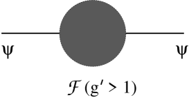
Figure 3: the grey ball stands for a non-perturbative correction depending on the strong coupling $g^{\prime}$.

Only when they have a perturbative description in terms of type I string, the heterotic hidden sectors need in fact to appear with a separation into charged sectors (on the D-branes) and uncharged sectors (the closed string). We know on the other hand that, in some way, the uncharged hypermultiplets of the closed string sector “feel” the D-branes, being, as the latter, in one-to-one correspondence with the orbifold fixed points: it is therefore not too surprising that this effect is emphasized at the strong coupling. We may ask how is it possible that a gauge group that in a weak coupling string description has a positive beta function, at the strong coupling has instead an opposite behavior under renormalization. The positiveness of the beta function is due to a predominancy of the hypermultiplets contribution, through diagrams of the type 2), with respect to the vector contribution, given by diagrams of the type 1) of figure 4.

Figure 4: the diagrams contributing to the one-loop beta function.

At the strong coupling, the asymptotic states in the “hypermultiplets” are on the other hand forced to bound into singlets of the gauge group. The “elementary” vertices of bosons and matter states, whose coupling is the charge of the matter states, are now expected to vanish. This means that vertices of the type 2) should now be suppressed with respect to the diagrams of the type 1). It is therefore reasonable to expect a change in the sign of the “beta-function”. We stress however that these arguments have to be taken with extreme care, being only extremely qualitative.

We are now in the position to reconsider the puzzle of the apparent insensitivity of the string gauge threshold corrections to the existence (i.e. masslessness) of the hidden sector, in contrast with the dependence on their coupling. It is now clear that we cannot anymore rely on “index” theorems in order to compute such corrections: at a generic point in the K3 moduli space, ${\cal N}_{4}=2$ supersymmetry may not exist. We are therefore not allowed to advocate supersymmetry in order to exclude any dependence of the threshold corrections on the K3 moduli, and promote the result of the computation performed at an orbifold point, to a general result valid at any point of the K3. Actually, the explicit results sofar obtained for the heterotic string, have been computed at the $Z_{2}$ orbifold point [45]. This is a very special point in the hypermultiplets moduli, and there is no surprise that precisely at that point the hidden sectors are massless. In fact, at this point the hypermultiplet moduli are twisted; it is very likely that the masslessness of the hidden sectors is related to this, as much as the two Horava–Witten walls providing the two $E_{8}$ give rise to massless states only when the eleventh coordinate is twisted. If, away from the $Z_{2}$ orbifold point, supersymmetry is broken, nothing prevents the moduli of K3 from contributing to the correction: very likely, the mass of the states of the hidden sectors acts as a suppression factor for the dependence of the threshold corrections on the gauge couplings of these sectors.

The above arguments, relating the non-vanishing of the beta-function to the breaking of supersymmetry, apply to the gauge coupling, but not to couplings like that of the $R^{2}$ term. More precisely, they don’t apply to the “modified” $R^{2}$ term, the gravitational amplitude considered in this work, and introduced in Ref. [14]. This amplitude is precisely defined by subtracting the “interaction” terms of the currents, accounting for true “loop effects” of the theory. The large-$T$, -$U$ contribution of the “hidden sectors” to this amplitude is therefore a “tree level” effect of the theory, that accounts for the presence of these extra sectors, “weighting” like the perturbative sector, and entering on the same footing. As we saw, the beta-function of this term is non-vanishing for all the cases considered in sections 4.1–4.7.

6 Conclusions

In this work we have considered type II/heterotic/type I string–string duality for constructions with perturbative ${\cal N}=4$ and ${\cal N}=2$ supersymmetry in four dimensions. Our aim was to investigate some non-perturbative properties of string theory by using as source of information the various dual string constructions. In all the cases we considered, there exists a region in the moduli space that corresponds to a weak coupling regime at the same time in the type I, type II and heterotic strings. For any example, we have therefore considered the theory from all the three dual points of view: no one of these single approaches can in fact capture at once all the aspects of a construction. The existence of a common region of weak coupling does not mean that the theory has to look the same in all the three dual string approaches: the existence of non-perturbative states present for any value of the string coupling makes in some cases the identification of dual constructions and the test of duality quite subtle. In such cases, an analysis based on a naive comparison of the moduli spaces can be misleading, being necessarily affected by the identification of the associated effective theories. We therefore performed the analysis at the $Z_{2}$ orbifold point, where we can explicitly write the partition function and compute string threshold corrections. The comparison of the renormalization of certain couplings of the effective action allows us to point out several novel features, that in certain cases lead to an identification of duals slightly different from what previously proposed, thereby changing the perspective of the duality map between string constructions. Among the cases considered, particularly relevant are those in which part of the string massless spectrum is non-perturbative from the heterotic and/or type I point of view. These provide explicit examples of the situations considered in Refs. [38, 41], of four dimensional heterotic theories obtained by toroidal compactification on $T^{2}$ of a six dimensional theory, in which however the ${\cal N}_{4}=2$ heterotic non-perturbative massless spectrum does not fit with the anomaly constraint of ${\cal N}=1$ field theory in six dimensions. The investigation of these theories from the dual type II point of view makes clear that, although from the heterotic point of view the ${\cal N}_{4}=2$ theory is just obtained by toroidal compactification of ${\cal N}_{6}=1$, in their whole these theories cannot be defined in six dimensions, in the sense that the massless states cannot be represented all at the same time in terms of an effective ${\cal N}_{6}=1$ field theory. The mismatch is on the other hand in a part of the spectrum which is non-perturbative from the heterotic point of view: there is therefore no contradiction with the field theory constraints, that control only the perturbative part of the heterotic string, the one corresponding to a six dimensional supergravity description. Indeed, in the case of ${\cal N}_{4}=2$ orbifolds, we found an intriguing relation between i) the T-duality of the heterotic string, that exchanges the Kähler class and complex structure moduli, resp. $T$ and $U$, of the two torus, ii) the modular invariance on the type II side, that implies a symmetry between different orbifold twisted sectors, and iii) the type I symmetry between D9- and D5-branes sectors. For string theory, modular invariance is a more fundamental property than anomaly cancellation in the associated effective action; only when one considers just the perturbative string spectrum the two requirements in some cases turn out to be equivalent. The counter-example is provided by the above mentioned situations. There, only a part of the heterotic string spectrum satisfies $d=6$ anomaly cancellation constraints, and admits a representation in terms of an effective supergravity also when decompactified to six dimensions. Nevertheless, the string theory is well defined; in particular, the massless spectrum is consistent with pure string theory requirements, such as modular invariance, or T-duality, or tadpoles cancellation. These properties, intriguingly related each other and, ultimately, to the renormalizability of string theory, are non-trivially interchanged under string–string duality.

Another pure stringy phenomenon, that does not have a field theory counterpart, is the “interaction” of perturbative and “hidden”, non-perturbative sectors, that takes place whenever in the heterotic, or type I string, some gauge group factors possess a non-vanishing beta-function. The kind of interaction between sectors is rather peculiar and cannot be written in terms of an effective field theory with multi-dilaton gauge sectors. Indeed, the expressions of the threshold corrections suggest that in such cases the hidden sector is at the strong coupling. As a consequence, supersymmetry is broken by gaugino condensation in the hidden sectors. This scenario is compatible with a perturbatively supersymmetric construction, because the supersymmetry breaking terms are non-perturbative from the point of view of the “visible” sector. We only devoted some qualitative comments to this phenomenon, that definitely deserves a deeper understanding and further investigation. A consequence of this is in fact the general breaking to ${\cal N}=0$ in the heterotic string with ${\cal N}_{4}=1$.

With this work, we hope at least to have made clear the urgency of looking at string theory by avoiding as much as possible any short cut provided by a heavy use of the properties of its representations in terms of supersymmetric field theories, an approach sometimes misleading.

Acknowledgments

I am grateful to Jean–Pierre Derendinger and to Robert Helling for valuable discussions. I also acknowledge the kind hospitality of the Department of Physics of the University of Neuchâtel and the Swiss National Science Foundation for partial financial support.

References

- [1] A. Gregori, C. Kounnas, and J. Rizos, Classification of the N = 2, Z(2) x Z(2)-symmetric type II orbifolds and their type II asymmetric duals, Nucl. Phys. B549 (1999) 16–62, hep-th/9901123.
- [2] E. Witten, String theory dynamics in various dimensions, Nucl. Phys. B443 (1995) 85–126, hep-th/9503124.
- [3] J. Polchinski and E. Witten, Evidence for Heterotic - Type I String Duality, Nucl. Phys. B460 (1996) 525–540, hep-th/9510169.
- [4] S. Kachru and C. Vafa, Exact results for N=2 compactifications of heterotic strings, Nucl. Phys. B450 (1995) 69–89, hep-th/9505105.
- [5] A. Klemm, W. Lerche, and P. Mayr, K3 Fibrations and heterotic type II string duality, Phys. Lett. B357 (1995) 313–322, hep-th/9506112.
- [6] P. S. Aspinwall and J. Louis, On the Ubiquity of K3 Fibrations in String Duality, Phys. Lett. B369 (1996) 233–242, hep-th/9510234.
- [7] S. Kachru, A. Klemm, W. Lerche, P. Mayr, and C. Vafa, Nonperturbative results on the point particle limit of N=2 heterotic string compactifications, Nucl. Phys. B459 (1996) 537–558, hep-th/9508155.
- [8] D. R. Morrison and C. Vafa, Compactifications of F-Theory on Calabi–Yau Threefolds – I, Nucl. Phys. B473 (1996) 74–92, hep-th/9602114.
- [9] D. R. Morrison and C. Vafa, Compactifications of F-Theory on Calabi–Yau Threefolds – II, Nucl. Phys. B476 (1996) 437–469, hep-th/9603161.
- [10] E. Witten, Small Instantons in String Theory, Nucl. Phys. B460 (1996) 541–559, hep-th/9511030.
- [11] P. S. Aspinwall and D. R. Morrison, Point-like instantons on K3 orbifolds, Nucl. Phys. B503 (1997) 533–564, hep-th/9705104.
- [12] P. S. Aspinwall, K3 surfaces and string duality, hep-th/9611137.
- [13] P. Mayr, N = 1 heterotic string vacua from mirror symmetry, hep-th/9904115.
- [14] A. Gregori, C. Kounnas, and P. M. Petropoulos, Non-perturbative gravitational corrections in a class of N = 2 string duals, Nucl. Phys. B537 (1999) 317–343, hep-th/9808024.
- [15] A. Gregori, C. Kounnas, and P. M. Petropoulos, Non-perturbative triality in heterotic and type II N = 2 strings, Nucl. Phys. B553 (1999) 108–132, hep-th/9901117.
- [16] A. Gregori and C. Kounnas, Four-dimensional N = 2 superstring constructions and their (non-)perturbative duality connections, Nucl. Phys. B560 (1999) 135–153, hep-th/9904151.
- [17] J. A. Harvey and G. Moore, Algebras, BPS States, and Strings, Nucl. Phys. B463 (1996) 315–368, hep-th/9510182.
- [18] I. Antoniadis, E. Gava, and K. S. Narain, Moduli corrections to gravitational couplings from string loops, Phys. Lett. B283 (1992) 209–212, hep-th/9203071.
- [19] I. Antoniadis, E. Gava, and K. S. Narain, Moduli corrections to gauge and gravitational couplings in four-dimensional superstrings, Nucl. Phys. B383 (1992) 93–109, hep-th/9204030.
- [20] J. F. Morales and M. Serone, BPS states and supersymmetric index in N = 2 type I string vacua, Nucl. Phys. B501 (1997) 427–444, hep-th/9703049.
- [21] M. J. Duff and R. R. Khuri, Four-dimensional string / string duality, Nucl. Phys. B411 (1994) 473–486, hep-th/9305142.
- [22] C. M. Hull and P. K. Townsend, Unity of superstring dualities, Nucl. Phys. B438 (1995) 109–137, hep-th/9410167.
- [23] E. G. Gimon and J. Polchinski, Consistency Conditions for Orientifolds and D-Manifolds, Phys. Rev. D54 (1996) 1667–1676, hep-th/9601038.
- [24] A. Gregori et al., R**2 corrections and non-perturbative dualities of N = 4 string ground states, Nucl. Phys. B510 (1998) 423–476, hep-th/9708062.
- [25] E. Kiritsis, N. A. Obers, and B. Pioline, Heterotic/type II triality and instantons on K3, JHEP 01 (2000) 029, hep-th/0001083.
- [26] J. A. Harvey and G. Moore, Fivebrane instantons and R**2 couplings in N = 4 string theory, Phys. Rev. D57 (1998) 2323–2328, hep-th/9610237.
- [27] E. Kiritsis and C. Kounnas, Infrared regularization of superstring theory and the one loop calculation of coupling constants, Nucl. Phys. B442 (1995) 472–493, hep-th/9501020.
- [28] I. Antoniadis, E. Dudas, and A. Sagnotti, Supersymmetry breaking, open strings and M-theory, Nucl. Phys. B544 (1999) 469–502, hep-th/9807011.
- [29] I. Antoniadis, G. D’Appollonio, E. Dudas, and A. Sagnotti, Partial breaking of supersymmetry, open strings and M- theory, Nucl. Phys. B553 (1999) 133–154, hep-th/9812118.
- [30] S. Ferrara, J. A. Harvey, A. Strominger, and C. Vafa, Second quantized mirror symmetry, Phys. Lett. B361 (1995) 59–65, hep-th/9505162.
- [31] J. A. Harvey and G. Moore, Exact gravitational threshold correction in the FHSV model, Phys. Rev. D57 (1998) 2329–2336, hep-th/9611176.
- [32] C. Vafa and E. Witten, On orbifolds with discrete torsion, J. Geom. Phys. 15 (1995) 189–214, hep-th/9409188.
- [33] M. Bianchi and A. Sagnotti, Twist symmetry and open string Wilson lines, Nucl. Phys. B361 (1991) 519–538.
- [34] M. Berkooz et al., Anomalies, Dualities, and Topology of D=6 N=1 Superstring Vacua, Nucl. Phys. B475 (1996) 115–148, hep-th/9605184.
- [35] G. Aldazabal, A. Font, L. E. Ibanez, and F. Quevedo, Heterotic/Heterotic Duality in D=6,4, Phys. Lett. B380 (1996) 33–41, hep-th/9602097.
- [36] I. Antoniadis, H. Partouche, and T. R. Taylor, Duality of N = 2 heterotic-type I compactifications in four dimensions, Nucl. Phys. B499 (1997) 29–44, hep-th/9703076.
- [37] L. J. Dixon, V. Kaplunovsky, and J. Louis, Moduli dependence of string loop corrections to gauge coupling constants, Nucl. Phys. B355 (1991) 649–688.
- [38] A. Gregori, Rank 48 gauge group in heterotic string, hep-th/0010086.
- [39] I. Antoniadis, C. Bachas, C. Fabre, H. Partouche, and T. R. Taylor, Aspects of type I - type II - heterotic triality in four dimensions, Nucl. Phys. B489 (1997) 160–178, hep-th/9608012.
- [40] P. S. Aspinwall and M. R. Plesser, T-duality can fail, JHEP 08 (1999) 001, hep-th/9905036.
- [41] A. Gregori, The d = 6, N = 1 heterotic string does not ’live’ in six dimensions, hep-th/0110025.
- [42] G. Curio and D. Lust, A class of N = 1 dual string pairs and its modular superpotential, Int. J. Mod. Phys. A12 (1997) 5847–5866, hep-th/9703007.
- [43] B. Andreas, G. Curio, and D. Lust, N = 1 dual string pairs and their massless spectra, Nucl. Phys. B507 (1997) 175–196, hep-th/9705174.
- [44] A. Gregori, On the strong coupling behavior of heterotic and type I orbifolds, hep-th/0005124.
- [45] E. Kiritsis, C. Kounnas, P. M. Petropoulos, and J. Rizos, Universality properties of N = 2 and N = 1 heterotic threshold corrections, Nucl. Phys. B483 (1997) 141–171, hep-th/9608034.
- [46] M. J. Duff, R. Minasian, and E. Witten, Evidence for Heterotic/Heterotic Duality, Nucl. Phys. B465 (1996) 413–438, hep-th/9601036.
- [47] A. Sen and C. Vafa, Dual pairs of type II string compactification, Nucl. Phys. B455 (1995) 165–187, hep-th/9508064.
- [48] E. Kiritsis, C. Kounnas, P. M. Petropoulos, and J. Rizos, String threshold corrections in models with spontaneously broken supersymmetry, Nucl. Phys. B540 (1999) 87–148, hep-th/9807067.
- [49] P. Horava and E. Witten, Heterotic and type I string dynamics from eleven dimensions, Nucl. Phys. B460 (1996) 506–524, hep-th/9510209.
- [50] P. Horava and E. Witten, Eleven-Dimensional Supergravity on a Manifold with Boundary, Nucl. Phys. B475 (1996) 94–114, hep-th/9603142.
- [51] I. Antoniadis, J. P. Derendinger, and C. Kounnas, Non-perturbative temperature instabilities in N = 4 strings, Nucl. Phys. B551 (1999) 41–77, hep-th/9902032.
- [52] R. Dijkgraaf, E. Verlinde, and H. Verlinde, C=1 conformal fields theories on Riemann surfaces, Comm. Math. Phys. 115 (1988) 2264.
- [53] M. Bianchi, A note on toroidal compactifications of the type I superstring and other superstring vacuum configurations with 16 supercharges, Nucl. Phys. B528 (1998) 73–94, hep-th/9711201.
- [54] C. Angelantonj, Comments on open-string orbifolds with a non-vanishing B(ab), Nucl. Phys. B566 (2000) 126–150, hep-th/9908064.
- [55] Z. Kakushadze, G. Shiu, and S. H. H. Tye, Type IIB orientifolds with NS-NS antisymmetric tensor backgrounds, Phys. Rev. D58 (1998) 086001, hep-th/9803141.
- [56] E. Kiritsis, C. Kounnas, P. M. Petropoulos, and J. Rizos, Solving the decompactification problem in string theory, Phys. Lett. B385 (1996) 87–95, hep-th/9606087.
- [57] M. Dine, R. Rohm, N. Seiberg, and E. Witten, GLUINO CONDENSATION IN SUPERSTRING MODELS, Phys. Lett. B156 (1985) 55.
- [58] C. P. Burgess, J. P. Derendinger, F. Quevedo, and M. Quiros, Gaugino condensates and chiral linear duality: An Effective Lagrangian analysis, Phys. Lett. B348 (1995) 428–442, hep-th/9501065.
- [59] C. P. Burgess, J. P. Derendinger, F. Quevedo, and M. Quiros, On gaugino condensation with field-dependent gauge couplings, Annals Phys. 250 (1996) 193, hep-th/9505171.