hep-th/0110200

UT-972

October, 2001

D-branes in Melvin Background

Tadashi Takayanagi and Tadaoki Uesugi

Department of Physics, Faculty of Science
University of Tokyo
Tokyo 113-0033, Japan

In this paper we discuss D-branes in the Melvin background and its supersymmetric generalizations. In particular we determine the D-brane spectra in these backgrounds by constructing their boundary states explicitly, where some of the D-branes are supersymmetric. The results sensitively depend on whether the value of magnetic flux in the Melvin background is rational or irrational. For the rational case the D-branes are regarded as the generalizations of fractional D-branes in abelian orbifolds ${\bf C^{n}/Z_{N}}$ of type II or type 0 string theory. For the irrational case we found a very limited spectrum. Since the background includes the nontrivial H-flux, the D-branes will provide interesting examples from the viewpoint of the noncommutative geometry.

1 Introduction

One of the important problems in string theory is to understand its vacuum structure completely. Some recent discoveries have revealed the connections between the several vacua whose definitions were originally thought to be different from each other. The first great advance came with the discovery of the string duality [1]. The five string ‘theories’ in flat space turned out to be not different theories but different vacua in a single theory, that is to say, M-theory. The second advance has been made from the investigation of the open string tachyon condensation on unstable and thus non-supersymmetric D-brane systems (for a review see [2, 3]). The key idea of understanding this phenomenon is the Sen’s conjecture, which says that the unstable vacuum with D-branes decays to stable lower dimensional D-branes or the closed string vacuum. From this we can expect that the original vacuum with the unstable D-brane system belongs to the spontaneous supersymmetry broken phase. Indeed the nonlinear supersymmetries can be realized on such systems [4, 5].

From this we expect that the above observation about open string unstable systems may be applied to closed string unstable vacua such as type 0 string etc. (for the type 0 theory see [6]). If we naively translate the above statement into those examples, such closed string ‘theories’ are not different theories from type II but only different vacua. One attempt in this direction will be the conjecture that type 0A string is equivalent to ${\bf S}^{1}$ compactification of M-theory with the anti-periodic boundary condition for all fermions [7]. Moreover we may speculate that the type 0 string is a spontaneously broken phase of the original thirty two supersymmetries in type II, where the gravitino may obtain the infinite mass and thus disappear. However, in reality it seems difficult to explain it completely within the framework of classical supergravity. For example, one should explain the presence of tachyon in type 0 string and the doubling of RR-fields. These intriguing questions about unstable closed string vacua will also be closely related to the closed string tachyon condensation, which remains to be well understood (for latest discussions see e.g [8, 9, 10, 11, 12, 13, 14]).

Recently the Kaluza-Klein Melvin backgrounds [15, 16, 17, 18] have been intensively studied both in M-theory (or superstring with RR flux) [19, 20, 9, 21, 22, 23, 24, 25, 26, 27, 28] and in NS-NS superstring model [29, 30, 19, 12, 13, 14]. Both backgrounds will provide useful materials for the studies of unstable closed string vacua since these are known to connect type 0 string with type II string in the flat space [19]. In the former context the Melvin-like solutions are called flux-branes (Fp-brane) [20, 9, 21, 22]. On the other hand, the latter model gives an exactly solvable superstring model in spite of its non-trivial curved background with $H$-flux [29, 30, 13, 14]. The simplest model [29, 30] (‘9-11’ flip of F7-brane) includes three parameters (the radius $R$ and two magnetic fluxes $q$ and $\beta$) and thus does cover many vacua. In particular, by tuning these parameters appropriately we can realize the type 0 or type II string and this shows explicitly that the Melvin background connects type 0 with type II. Furthermore it can be shown that all of the abelian orbifolds ${\bf C}/{\bf Z}_{N}$ in type 0 or type II string are also included as special limits [13]. We can also construct supersymmetric Melvin backgrounds [13, 14] by considering the higher dimensional generalizations (‘9-11’ flip of F5, F3 and F1-brane). These also include supersymmetric orbifolds such as ALE orbifolds ${\bf C}^{2}/{\bf Z}_{N}$ (for ALE space see [31]) as well as nonsupersymmetic orbifolds. These Melvin models describe a large region of string vacua both supersymmetric and nonsupersymmetic, interpolating various orbifolds. Therefore these models will be suitable to explore the structure of vacua in string theory and the decay of unstable vacua.

If we are given a non-trivial background like one of these, a D-brane generally provides a good probe to investigate its stringy geometry. Thus in this paper we will discuss various aspects of D-branes in the Melvin backgrounds. Because the model is exactly solvable as we have mentioned, the boundary conformal field theories of D-branes are also treated exactly. In particular we can construct their boundary states explicitly as we will see later. As a result we find that these D-branes depend on the parameters of the Melvin background in intriguing ways. For example, if we assume the simplest Melvin model [29, 30] and the parameters $qR$ and $\frac{\beta\alpha^{\prime}}{R}$ are rational numbers, the D-branes which wrap the compactified circle depend only on $qR$, while those which are point-like along the circles depend only on $\frac{\beta\alpha^{\prime}}{R}$. This difference sometimes causes the strange Bose-Fermi degeneracy in the open string spectrum on the D-branes in spite of the absence of supersymmetry in the closed string sector. We will later discuss an interpretation of this degeneracy as a remnant of the spontaneously broken supersymmetry.

Even though these two kinds of D-branes are transformed into each other by T-duality, they look different geometrically. The former kind of the D-brane has the spiral world-volume wrapping several times on two dimensional tori like coils. On the other hand, the latter kind of the D-brane is very similar to fractional D-branes [32, 33] in orbifold theories. Indeed as we have mentioned, if we take appropriate limits, then the model becomes equivalent to orbifolds ${\bf C}/{\bf Z}_{N}$ in type 0 and type II string. We can see that the D-branes in the Melvin background really become the fractional D-branes in the orbifold limit. Especially we find that a D-brane in the Melvin model is divided into an electric fractional D-brane and a magnetic fractional D-brane [34, 35, 36, 7, 37] in the type 0 limit. We also find an interesting phenomenon that the type of a fractional-like D-brane is changed due to a kind of monodromy if it goes around the circle.

Moreover, D-brane spectra are very sensitive to whether the magnetic parameters $qR$ and $\frac{\beta\alpha^{\prime}}{R}$ are rational or irrational. It was found that if we take the decompactified limit in the irrational case, then the closed string sector approaches not the ordinary orbifold ${\bf C}/{\bf Z}_{N}$ but an unfamiliar kind of a ‘large $N$ limit of the orbifold’ [13]. In this case all of the allowed D-branes are pinned at the fixed point of the Melvin background and cannot move around, while in the rational case there exist movable D-branes similar to those which belong to the regular representations in the orbifold theories. Indeed for the irrational parameters if we would try to move the D-branes away which wrap the compactified circle, it should wind infinitely many times (‘foliation’) and thus it becomes singular.

In this way the D-branes in Melvin backgrounds change their aspects dramatically in accordance with the various values of magnetic parameters.

It will also be an interesting result that if we consider the higher dimensional supersymmetric Melvin backgrounds [13, 14], then we can obtain BPS D-branes. In the orbifold limit these D-branes are identified with BPS fractional D-branes on ALE orbifolds ${\bf C}^{2}/{\bf Z}_{N}$.

Finally we would like to mention another interesting viewpoint on the Melvin backgrounds. They include non-trivial $H$-flux for non-zero $\beta$ and thus the world-volume theory on the D-branes in these backgrounds may be analyzed in terms of noncommutative geometry [38, 39, 40]. Related examples from this viewpoint may be the D-branes in group manifolds [41, 42], where the non-trivial $H$-flux is also present. Recently the D-brane charges of these [43] are explained by employing twisted K-theory [44] in [45, 46].

The plan of this paper is as follows. In section two we review the Melvin background and the quantization of its sigma model by the operator method. In section three we investigate the D-branes in the Melvin background by using the boundary state formalism. We calculate the vacuum amplitude and check the open-closed duality relation. We discuss the geometrical properties of them. We also examine the relation to fractional D-branes in orbifold theories. In section four we generalize the arguments in section three to those of the higher dimensional Melvin model. We see that the D-branes in this background become supersymmetric for specific values of the parameters. In section five we draw conclusions and discuss the future problems. In appendix we summarize some known facts which are necessary for the analysis in this paper.

2 Closed Strings in the Melvin Background

In this section we mainly review the exactly solvable model of type II superstring studied in [29, 30] as well as some recent related developments [19, 7, 13]. See also [47, 48, 49] for such a model in bosonic string theory. We also present the detailed analysis of the world-sheet fermions in NS-R formalism by using superfields.

The target space of this model has the structure of Kaluza-Klein theory and has the topology $\mbox{M}_{3}\times{\bf R}^{1,6}$. The three dimensional manifold $\mbox{M}_{3}$ is given by ${\bf S}^{1}$ fibration over ${\bf R}^{2}$. We write the coordinate of ${\bf R}^{2}$ and ${\bf S}^{1}$ by $\rho,\varphi$ (polar coordinate) and $y$ (with radius $R$). This non-trivial fibration is due to two Kaluza-Klein (K.K.) gauge fields $A_{\varphi}$ and $B_{\varphi}$ (see eq.(2)) which originate from K.K. reduction of metric $G_{\varphi y}$ and B-field $B_{\varphi y}$, respectively. Thus this background can be viewed as a generalization [16, 17] of the original Melvin solution [15] to string theory, which is recently discussed in the context of the flux brane [20, 21, 9, 22, 23, 24, 25, 27, 14, 28]. In the most of the discussions below, we will neglect the trivial flat part ${\bf R}^{1,6}$

The explicit metric and other NSNS fields before the Kaluza-Klein reduction are given as follows

$$ds^{2} = d\rho^{2}+\frac{\rho^{2}}{(1+\beta^{2}\rho^{2})(1+q^{2}\rho^{2})}d\varphi^{2}+\frac{1+q^{2}\rho^{2}}{1+\beta^{2}\rho^{2}}(dy+A_{\varphi}d\varphi)^{2},$$

$$A_{\varphi} = \frac{q\rho^{2}}{1+q^{2}\rho^{2}},\ \ \ B_{\varphi y}\equiv B_{\varphi}=-\frac{\beta\rho^{2}}{1+\beta^{2}\rho^{2}},\ \ \ e^{2(\phi-\phi_{0})}=\frac{1}{1+\beta^{2}\rho^{2}},$$ (2.1)

where $q,\beta$ are the magnetic parameters which are proportional to the strength of two gauge fields and $\phi_{0}$ is the constant value of the dilaton $\phi$ at $\rho=0$.

It would be useful to note that if $\beta=0$, we get a locally flat metric

$$ds^{2}=d\rho^{2}+dy^{2}+\rho^{2}(d\varphi+qdy)^{2}.$$ (2.2)

This background is globally non-trivial because the angle $\varphi$ is compactified such that its period is $2\pi$. For example, its geodesic lines $\varphi+qy=$const. are spiral and do not return to the same point for irrational $qR$ if one goes around the circle ${\bf S}^{1}$. As we will see later, this geometry rules the D-brane spectrum.

2.1 Sigma Model Description and Its Free Field Representation

At first sight the above background (2.1) for general $q,\beta$ does not seem to be tractable in the description of the two dimensional sigma model. However, with appropriate T-duality transformations which we will review in appendix A (see also [50]) one can solve this sigma model in terms of free fields [49, 29]. In this paper we define the coordinate of world-sheet as $z=\sigma_{1}+i\sigma_{2}$ and the derivatives as $\partial=\frac{1}{2}(\partial_{1}-i\partial_{2}),\bar{\partial}=\frac{1}{2}(\partial_{1}+i\partial_{2})$.

The sigma model for the background (2.1) is given by (we show only the bosonic part)

$$S = \frac{1}{\pi\alpha^{\prime}}\int d^{2}\sigma\Biggl{[}\bar{\partial}\rho\partial\rho+\frac{(1+q^{2}\rho^{2})}{(1+\beta^{2}\rho^{2})}(\bar{\partial}Y+\frac{q\rho^{2}}{1+q^{2}\rho^{2}}\bar{\partial}\varphi)(\partial Y+\frac{q\rho^{2}}{1+q^{2}\rho^{2}}\partial\varphi)$$

$$+\frac{\rho^{2}}{(1+\beta^{2}\rho^{2})(1+q^{2}\rho^{2})}\bar{\partial}{\varphi}\partial{\varphi}-\frac{\beta\rho^{2}}{1+\beta^{2}\rho^{2}}(\bar{\partial}Y\partial\varphi-\partial Y\bar{\partial}\varphi)\Biggr{]}$$

$$= \frac{1}{\pi\alpha^{\prime}}\int d^{2}\sigma\Biggl{[}\bar{\partial}\rho\partial\rho+\bar{\partial}Y\partial Y+\frac{\rho^{2}}{1+\beta^{2}\rho^{2}}(\bar{\partial}\varphi+(q-\beta)\bar{\partial}Y)(\partial\varphi+(q+\beta)\partial Y)\Biggr{]},$$

where we have omitted the term of the dilaton coupling for simplicity. We have also abbreviated the fermion terms since it is easily obtained if we use the superfield. They are easily incorporated if we use the ${\mathcal{N}}=1$ world-sheet superfield formulation.

First let us perform the T-duality which transforms the field $\varphi$ into the new one $\tilde{\varphi}$ (for more explanations see the appendix A). The result is given by

$$S = \frac{1}{\pi\alpha^{\prime}}\int d^{2}\sigma\Bigl{[}\bar{\partial}\rho\partial\rho+(\bar{\partial}Y+\beta\bar{\partial}\tilde{\varphi})(\partial Y+\beta\partial\tilde{\varphi})+q(\bar{\partial}\tilde{\varphi}\partial Y-\bar{\partial}Y\partial\tilde{\varphi})+\frac{1}{\rho^{2}}\bar{\partial}\tilde{\varphi}\partial\tilde{\varphi}\Bigr{]}.$$

After we define the field $Y^{\prime}$ by

$$Y^{\prime}=Y+\beta\tilde{\varphi},$$ (2.5)

we can again take the T-duality along $\tilde{\varphi}$ into $\varphi^{\prime}$. Then we obtain

$$S = \frac{1}{\pi\alpha^{\prime}}\int d^{2}\sigma\Bigl{[}\bar{\partial}\rho\partial\rho+\bar{\partial}Y^{\prime}\partial Y^{\prime}+\rho^{2}(\bar{\partial}\varphi^{\prime}+q\bar{\partial}Y^{\prime})(\partial\varphi^{\prime}+q\partial Y^{\prime})\Bigr{]}.$$ (2.6)

From this expression it is easy to see that one can describe the sigma model by free fields $X^{\prime}$ and $\bar{X}^{\prime}$ which are defined by

$$X^{\prime}=\rho e^{i\varphi^{\prime\prime}},~{}\bar{X}^{\prime}=\rho e^{-i\varphi^{\prime\prime}},$$ (2.7)

where

$$\varphi^{\prime\prime}=\varphi^{\prime}+qY^{\prime}.$$ (2.8)

Here we will examine the relation between the free fields $X^{\prime},\bar{X}^{\prime}$ and the fields $X=\rho e^{i\varphi},\bar{X}=\rho e^{-i\varphi}$ which represent the original plane ${\bf R^{2}}\in\mbox{M}_{3}$ in (2.1). Applying the relation (A.6) to the above two different T-duality transformations, we can obtain

$$\partial\varphi=\partial\varphi^{\prime\prime}-q\partial Y-\beta\partial Y^{\prime},\ \ \ \bar{\partial}\varphi=\bar{\partial}\varphi^{\prime\prime}-q\bar{\partial}Y+\beta\bar{\partial}Y^{\prime}.$$ (2.9)

This shows that the field $\varphi$ is rewritten as

$$\varphi(z,\bar{z})=\varphi^{\prime\prime}(z,\bar{z})-qY(z,\bar{z})+\beta\left(Y^{\prime}_{R}(\bar{z})-Y^{\prime}_{L}(z)\right),$$ (2.10)

where $Y^{\prime}_{L}(z)~{}(Y^{\prime}_{R}(\bar{z}))$ is the left(right)-moving part of $Y^{\prime}$. Therefore from this the relation between $X^{\prime},\bar{X}^{\prime}$ and $X,\bar{X}$ is represented as

$$X(z,\bar{z})=e^{-iqY(z,\bar{z})+i\beta Y^{\prime}_{R}(\bar{z})-i\beta Y^{\prime}_{L}(z)}X^{\prime}(z,\bar{z}).$$ (2.11)

It is easy to generalize the above results into those in the supersymmetric case since we can use ${\mathcal{N}}=1$ world-sheet superfield formulation. Then the above equation (2.11) does hold as a superfield and we can also define the free fields ($\psi^{\prime}_{L,R},\bar{\psi}^{\prime}_{L,R}$) as the partners of $(X^{\prime},\bar{X}^{\prime})$.

Since we have the free field representation $(Y^{\prime},\eta^{\prime}_{L,R})$, $(X^{\prime},\psi_{L,R})$ and $(\bar{X}^{\prime},\bar{\psi}_{L,R})$, the quantization of the Melvin background can be performed. Before that, we have to examine the boundary condition of the field $Y^{\prime}$, which is a little subtle analysis in this section. From the relations (A.7) one obtains

$$\partial\tilde{\varphi}=-\rho^{2}\partial\varphi^{\prime\prime}+i\psi^{\prime}_{L}\bar{\psi}^{\prime}_{L}\equiv i\alpha^{\prime}j_{L},$$

$$\bar{\partial}\tilde{\varphi}=\rho^{2}\bar{\partial}\varphi^{\prime\prime}-i\psi^{\prime}_{R}\bar{\psi}^{\prime}_{R}\equiv-i\alpha^{\prime}j_{R},$$ (2.12)

and the conservation law of the above current $j_{L,R}$ follows directly. Notice also the useful relation

$$\rho^{2}\partial\varphi^{\prime\prime}=\frac{1}{2i}(\bar{X}^{\prime}\partial X^{\prime}-X^{\prime}\partial\bar{X}^{\prime}).$$ (2.13)

Then we can define the angular momentum operators $\hat{J}_{L},\hat{J}_{R}$ in $(X^{\prime},\bar{X}^{\prime})\in{\bf R^{2}}$ directions as follows

$$\hat{J}_{L}=\frac{1}{2\pi i}\oint dz\ j_{L}(z),\ \ \hat{J}_{R}=-\frac{1}{2\pi i}\oint d\bar{z}\ j_{R}(\bar{z}).$$ (2.14)

Then we can see from (2.1) and (2.14) how the boundary condition of $\tilde{\varphi}$ should be twisted

$$\tilde{\varphi}(\tau,\sigma+2\pi)=\tilde{\varphi}(\tau,\sigma)-2\pi\alpha^{\prime}\hat{J},$$ (2.15)

where we have defined the total angular momentum operator as $\hat{J}=\hat{J}_{R}+\hat{J}_{L}$ and the new world-sheet coordinates $\tau,\sigma$ as $z=\exp{(\tau+i\sigma)}$. Moreover notice that the original coordinate $Y$ satisfies

$$Y(\tau,\sigma+2\pi)=Y(\tau,\sigma)+2\pi Rw.$$ (2.16)

After all from (2.5), (2.15) and (2.16) the periodicity of the field $Y^{\prime}$ is given by

$$Y^{\prime}(\tau,\sigma+2\pi)=Y^{\prime}(\tau,\sigma)+2\pi Rw-2\pi\alpha^{\prime}\beta\hat{J}.$$ (2.17)

On the other hand, the canonical momentum of $Y$ is

$$P_{Y} = \frac{1}{2\pi\alpha^{\prime}}\int d\sigma(q\bar{\partial}\tilde{\varphi}-q\partial\tilde{\varphi}+\partial Y^{\prime}+\bar{\partial}Y^{\prime})$$ (2.18)

$$= q\hat{J}+\frac{1}{2}(P^{\prime}_{L}+P^{\prime}_{R}),$$

where the first line is obtained from (LABEL:SG2) and (2.5). Therefore from the quantization of $P_{Y}$ as $P_{Y}=\frac{n}{R}~{}(n\in{\bf Z})$ the quantized zero modes of $Y^{\prime}$ are obtained as follows

$$P^{\prime}_{L}+P^{\prime}_{R}=2(\frac{n}{R}-q\hat{J}),\ \ P^{\prime}_{L}-P^{\prime}_{R}=2(\frac{Rw}{\alpha^{\prime}}-\beta\hat{J}).$$ (2.19)

Next we turn to the quantization of the free fields $X^{\prime},\bar{X}^{\prime}$ and $\psi^{\prime}_{L,R},\bar{\psi}^{\prime}_{L,R}$. They obey the following twisted boundary conditions which can be obtained from (2.11), (2.16) and (2.19),

$$X^{\prime}(\tau,\sigma+2\pi) = e^{2\pi i\gamma}X^{\prime}(\tau,\sigma),$$

$$\psi^{\prime}_{L}(\tau,\sigma+2\pi) = e^{2\pi i\gamma}\psi_{L}^{\prime}(\tau,\sigma),\ \ \ \psi^{\prime}_{R}(\tau,\sigma+2\pi)=e^{2\pi i\gamma}\psi_{R}^{\prime}(\tau,\sigma),$$ (2.20)

where $$~{}\gamma\equiv qRw+\beta\alpha^{\prime}(\frac{n}{R}-q\hat{J}).$$ (2.21)

Note that there are no zero-modes for $X^{\prime},\bar{X}^{\prime}$ if $\gamma$ is not an integer. This fact is crucial when we will consider D-branes in this model later.

The above boundary conditions are similar to those in orbifold theories and therefore it is straightforward to perform the mode expansion and its canonical quantization. We summarize these results in the appendix B.

2.2 Mass Spectrum

We have explained that the sigma model of the Melvin background can be solved in terms of free fields $(X^{\prime},\bar{X}^{\prime},Y^{\prime})$. Thus it is straightforward to compute the mass spectrum of this model in the NS-R formalism, which can be obtained from $L_{0},\tilde{L}_{0}$ in (B.4). If we represent it by using $\hat{N}_{L,R}$ in (B) and $\hat{J}_{L,R}$ in (B), the result [29, 30, 13] is given by

$$\frac{\alpha^{\prime}M^{2}}{2} = \frac{\alpha^{\prime}}{2R^{2}}(n-qR\hat{J})^{2}+\frac{R^{2}}{2\alpha^{\prime}}(w-\frac{\alpha^{\prime}}{R}\beta\hat{J})^{2}+\hat{N}_{R}+\hat{N}_{L}-\hat{\gamma}(\hat{J}_{R}-\hat{J}_{L}),$$ (2.23)

$$~{}~{}~{}~{}~{}~{}~{}~{}~{}~{}~{}~{}~{}~{}~{}~{}~{}\mbox{where}~{}~{}~{}\hat{\gamma}\equiv\gamma-[\gamma],$$

with the level matching constraint

$$\hat{N}_{R}-\hat{N}_{L}-nw+[\gamma]\hat{J}=0,$$ (2.24)

where $[\gamma]$ denotes the integer part of $\gamma$. Moreover the GSO-projection for type II theory restricts the above spectrum, which causes a little subtlety [29, 30, 13]. For $2n\leq\gamma<2n+1~{}(n\in{\bf Z})$ it is the standard type II GSO-projection and the allowed spectra are those which give $\hat{N}_{L,R}$ the integer values for NSNS-sector. However, for $2n+1\leq\gamma<2n+2$ it is the reversed one, where $\hat{N}_{L,R}$ takes half-integer values for NSNS-sector. This fact can be seen from the one-loop partition function $Z(R,q,\beta)$ [29, 30, 13] of the Melvin background by comparing the NS-R formalism with the Green-Schwarz formalism, where GSO-projection is not needed. In fact the spectrum (2.23) and (2.24) are the same as those obtained in the Green-Schwarz formalism [29, 30, 13].

Next let us see some interesting symmetries of the partition function $Z(R,q,\beta)$. From the mass spectrum it is easy to show the T-duality relation (see also appendix A)

$$Z(R,q,\beta)=Z(\frac{\alpha^{\prime}}{R},\beta,q).$$ (2.25)

Note that the interchange of $q$ and $\beta$ corresponds to that of metric $G_{\varphi y}$ and $B$-field $B_{\varphi y}$, which is the essential part of T-duality transformation. Furthermore one can see the periodicity of $q$ and $\beta$

$$Z(R,q,\beta)=Z\left(R,q+\frac{2n_{1}}{R},\beta+\frac{2n_{2}R}{\alpha^{\prime}}\right)~{}~{}~{}~{}(n_{1},n_{2}\in{\bf Z}).$$ (2.26)

2.3 Supersymmetry Breaking and Relation to Type 0 Theory

This Melvin model does not preserve supersymmetry except the case $(qR,\alpha^{\prime}\beta/R)\in(2{\bf Z},2{\bf Z})$, which is equivalent to the ordinary type II theory in the flat space by the periodicity (2.26). This fact can be seen from the non-vanishing of the partition function $Z(R,q,\beta)$. This can also be understood at the level of supergravity. Let us assume $\beta=0$ for simplicity, then all of spin $1/2$ fermions which go around the circle ${\bf S}^{1}$ receive the phase factor $e^{\pm i\pi qR}$. Thus only for $qR\in 2{\bf Z}$ the Killing spinors do exist and the supersymmetry is preserved. This shows the string theoretic realization of Scherk-Schwarz compactification [51, 52, 53]. In this kind of (spacetime) supersymmetry breaking the local supersymmetry is preserved while the global supersymmetry is broken [51]. This fact can be found in the open string spectrum on the D-brane as we will see in the section 3. For $\beta=0$ and $q\neq 0$ a D-brane which follows the Dirichlet boundary condition for ${\bf S}^{1}$ has the Bose-Fermi degeneracy while a D-brane which follows the Neumann boundary condition does not show the degeneracy.

Thus this model does not preserve supersymmetry in general and it may be unstable. Indeed it has tachyons if neither $qR$ nor $\alpha^{\prime}\beta/R$ is an integer [29]. In particular, for $(qR,\alpha^{\prime}\beta/R)\in(2{\bf Z}+1,2{\bf Z})$, the model is identical to type IIA(B) theory twisted by $(-1)^{F_{S}}\cdot\sigma_{1/2}$ with radius $2R$ as shown in [19], which is also equivalent to type 0B(A) theory twisted by $(-1)^{F_{R}}\cdot\sigma_{1/2}$ with radius $\frac{\alpha^{\prime}}{R}$ [7]. Here the operators $F_{S},F_{R}$ and $\sigma_{1/2}$ represent the spacetime fermion number, the world-sheet right-moving fermion number and the half-shift operator on the circle ${\bf S^{1}}$. If we further take the small radius limit $R\to 0$, we obtain ten-dimensional type 0B(A) string theory [7] after we perform the T-duality. On the other hand, if we take the limit $R\to\infty$ with $\beta=0$, then the theory is identical to the ordinal ten dimensional type IIA(B) string theory.

This equivalence can be generalized to the Melvin background with the fractional values of the magnetic parameters [13]. For the specific fractional values $qR=\frac{k}{N},\ \ \beta=0$ (or $\frac{\beta\alpha^{\prime}}{R}=\frac{k}{N},\ q=0$) the Melvin model is equivalent to ${\bf Z}_{N}$ freely acting orbifolds. Furthermore if we take the limit $R\to 0$ (or $R\to\infty$), those are reduced to the abelian orbifolds ${\bf C}/{\bf Z}_{N}$ with a fixed point in type II theory (for even $k$) and in type 0 theory (for odd $k$). We summarize the result in Table.1.

$k$	type II orbifold (radius)	T-dualized orbifold (radius)
even	IIA(B)/$\sigma_{1/N}\cdot g\ \ \ \ (NR=\frac{N\alpha^{\prime}}{\tilde{R}})$	IIB(A)/$\tilde{\sigma}_{1/N}\cdot g\ \ \ \ (\frac{\alpha^{\prime}}{NR}=\frac{\tilde{R}}{N})$
odd	IIA(B)/$\sigma_{1/2N}\cdot g\ \ \ (2NR=\frac{2N\alpha^{\prime}}{\tilde{R}})$	0B(A)/$\{(-1)^{F_{R}}\cdot\sigma_{1/2},\ \tilde{\sigma}_{1/N}\cdot g\}\ \ \ \ (\frac{\alpha^{\prime}}{NR}=\frac{\tilde{R}}{N})$

Table 1: The equivalence of the IIA(B) Melvin background for $qR=\frac{k}{N},\beta=0$ with freely acting orbifolds. The operators $g=\exp{(2\pi i\frac{k}{N}\hat{J})}$, $\sigma_{\frac{1}{N}}$ and $\tilde{\sigma}_{\frac{1}{N}}$ represent the projection operator, $\frac{1}{N}$-shift operator in the circle and its dual operator, respectively.

3 D-branes in Melvin Background

In this section we consider D-branes in Melvin background (2.1). In the previous section we have seen that the nonlinear sigma model in the Melvin background can be exactly solved. By applying the T-duality in the curved space and by redefining appropriate target space variables, the nonlinear sigma model can be rewritten by the free fields with the nontrivial boundary conditions, and we can quantize this action in the same way as that in the flat space.

With regard to open strings the quantization process can be also performed by the usual method. By changing the boundary conditions of open strings we can obtain the various D-branes in the Melvin background, while the several constraints which can not be seen in the flat space arise due to the nontriviality of the Melvin geometry. In the arguments below we define the D$p$-brane as the D-brane which has $p+1$ Neumann boundary conditions and $9-p$ Dirichlet boundary conditions in terms of the free fields $(X^{\prime},\bar{X}^{\prime},Y^{\prime})$, not the original fields $(X,\bar{X},Y)$. The interpretation of such D-branes in the original coordinate $(X,\bar{X},Y)$ of the Melvin background (2.1) is somewhat complicated as we will discuss later.

One of the interesting results in this section is that the D-brane spectra dramatically change according to whether the parameters in Melvin background $qR$ and $\frac{\beta\alpha^{\prime}}{R}$ take the rational or irrational value. For example if $qR$ or $\frac{\beta\alpha^{\prime}}{R}$ is rational there exist some D-branes which are movable in the $(X,\bar{X})\in{\bf R^{2}}$ plane, while if both of these parameters take irrational values all D-branes are pinned at the origin in the Melvin geometry. The second interesting result is that some D-branes wrap the nontrivial cycle in the Melvin geometry. For example, some D1-branes wrap the geodesic lines $\varphi+qy=\mbox{constant}$ in the Melvin geometry without NSNS $B$-field (2.2), which is the natural result because such a configuration gives the minimal mass of the D-brane.

However, the most interesting argument about it is that these D1-branes have the ‘spiral’ configuration. These wrap ${\bf S^{1}}$ in the $Y$ direction, however the location of the end point of this D1-brane after wrapping one time on ${\bf S^{1}}$ is not the same as that of the start point. In other words its end point rotates from the starting point by some angle in the $(X,\bar{X})\in R^{2}$. After wrapping repeatedly, this configuration becomes something like a coil wrapping several times on the torus. If the parameter $qR$ of the Melvin background is rational, the end point of its D1-brane after wrapping several times on $S^{1}$ connects to the starting point, while if the parameter is irrational its end point never meets the starting point and D1-brane wraps on the torus infinite times and becomes singular because the effective tension of D1-brane diverges.

There is the other motivation to consider D-branes in the Melvin background. As we have seen in the previous section or in [13], by tuning magnetic parameters $qR$ and $\frac{\beta\alpha^{\prime}}{R}$ appropriately the various ten dimensional backgrounds which we already know can be realized, that is, type II, type 0 in flat space and these abelian orbifolds ${\bf C}/{\bf Z}_{N}$. Therefore, if we consider D-branes in the Melvin background, we may understand how the D-branes in the above various backgrounds are connected with each other.

In orbifold theories there exist two types of D-branes which are called the fractional D-brane and the bulk D-brane [32, 33]. What we will find is that the fractional D-branes and bulk D-branes correspond to the pinned and movable D-branes which we have mentioned, respectively. Moreover these D-branes prove to naturally correspond not only to the D-branes in type II theory in flat space but also the bound state of an electric D-brane and a magnetic D-brane in type 0 theory [34, 36, 37, 35, 55, 56]. We can verify this by the calculation of the tension and the vacuum amplitude etc. by the method of the boundary state formalism.

3.1 Boundary State in Melvin Background

In order to investigate D-branes in general conformal field theories, it is convenient to use the boundary state formalism. The boundary state is one way of the representations of D-branes in the closed string Hilbert space, and thus from this we can investigate the interactions between two D-branes and between a D-brane and closed strings.

From previous sections we have already known that the action for the Melvin background reduces to that written by free fields. Therefore the construction of the boundary state is similar to that in the flat space (see [57, 58] and references there in), or more precisely to that in orbifold theories [35, 59, 60, 61] even though the D-branes which we will construct have various new intriguing structures. Below we will omit the trivial oscillators for ${R^{1,6}}$ directions on the world-sheet. One can use either the light-cone or covariant formulation.

For the compactified direction $Y^{\prime}$, the usual Neumann or Dirichlet boundary conditions are allowed:

$$\mbox{Neumann}: \left\{\begin{array}[]{ccc}\partial_{\tau}Y^{\prime}|_{\tau=0}|B\rangle=0{}&\leftrightarrow&~{}(\frac{n}{R}-q\hat{J})|B\rangle=0,\ \ (\beta_{m}+\tilde{\beta}_{-m})|B\rangle=0,\\ (\eta^{\prime}_{L}-\epsilon\eta^{\prime}_{R})|_{\tau=0}|B\rangle=0{}&\leftrightarrow&~{}(\eta_{r}-i\epsilon\tilde{\eta}_{-r})|B\rangle=0,\end{array}\right.$$ (3.3)

$$\mbox{Dirichlet}: \left\{\begin{array}[]{ccc}\partial_{\sigma}Y^{\prime}|_{\tau=0}|B\rangle=0{}&\leftrightarrow&~{}(\frac{Rw}{\alpha^{\prime}}-\beta\hat{J})|B\rangle=0,\ \ (\beta_{m}-\tilde{\beta}_{-m})|B\rangle=0,\\ (\eta^{\prime}_{L}+\epsilon\eta^{\prime}_{R})|_{\tau=0}|B\rangle=0{}&\leftrightarrow&~{}(\eta_{r}+i\epsilon\tilde{\eta}_{-r})|B\rangle=0,\end{array}\right.$$ (3.6)

where $|B\rangle$ is the boundary state and the parameter $\epsilon$ takes the value $\pm 1$ which comes from open string boundary conditions for world-sheet fermions. Note that the zero mode for $Y^{\prime}$ is given by (2.19). For the directions $X^{\prime},\bar{X}^{\prime}$ the allowed boundary conditions are

$$\mbox{Neumann-Neumann}: \left\{\begin{array}[]{ccc}\partial_{\tau}X^{\prime}|_{\tau=0}|B\rangle=0{}&\leftrightarrow&~{}(\alpha_{m-\gamma}+\tilde{\alpha}_{-m+\gamma})|B\rangle=0,\\ \partial_{\tau}\bar{X}^{\prime}|_{\tau=0}|B\rangle=0{}&\leftrightarrow&~{}(\bar{\alpha}_{m+\gamma}+\bar{\tilde{\alpha}}_{-m-\gamma})|B\rangle=0,\\ (\psi^{\prime}_{L}-\epsilon\psi^{\prime}_{R})|_{\tau=0}|B\rangle=0{}&\leftrightarrow&~{}(\psi_{r-\gamma}-i\epsilon\tilde{\psi}_{-r+\gamma})|B\rangle=0,\\ (\bar{\psi}^{\prime}_{L}-\epsilon\bar{\psi}^{\prime}_{R})|_{\tau=0}|B\rangle=0{}&\leftrightarrow&~{}(\bar{\psi}_{r+\gamma}-i\epsilon\bar{\tilde{\psi}}_{-r-\gamma})|B\rangle=0,\end{array}\right.$$ (3.11)

$$\mbox{Dirichlet-Dirichlet}: \left\{\begin{array}[]{ccc}\partial_{\sigma}X^{\prime}|_{\tau=0}|B\rangle=0{}&\leftrightarrow&~{}(\alpha_{m-\gamma}-\tilde{\alpha}_{-m+\gamma})|B\rangle=0,\\ \partial_{\sigma}\bar{X}^{\prime}|_{\tau=0}|B\rangle=0{}&\leftrightarrow&~{}(\bar{\alpha}_{m+\gamma}-\bar{\tilde{\alpha}}_{-m-\gamma})|B\rangle=0,\\ (\psi^{\prime}_{L}+\epsilon\psi^{\prime}_{R})|_{\tau=0}|B\rangle=0{}&\leftrightarrow&~{}(\psi_{r-\gamma}+i\epsilon\tilde{\psi}_{-r+\gamma})|B\rangle=0,\\ (\bar{\psi}^{\prime}_{L}+\epsilon\bar{\psi}^{\prime}_{R})|_{\tau=0}|B\rangle=0{}&\leftrightarrow&~{}(\bar{\psi}_{r+\gamma}+i\epsilon\bar{\tilde{\psi}}_{-r-\gamma})|B\rangle=0,\end{array}\right.$$ (3.16)

where $\gamma$ is given by (LABEL:phase). Here we have to note that the Neumann-Dirichlet or Dirichlet-Neumann boundary conditions can be defined only if $\gamma$ takes integer or half-integer values. We will discuss these special cases in the last of next subsection. We would also like to stress that in the above arguments we have defined the Dirichlet or Neumann boundary conditions with respect to the free fields $(X^{\prime},\bar{X}^{\prime},Y^{\prime})$. These boundary conditions are not always equivalent to the Dirichlet or Neumann boundary conditions with respect to the original fields $(X,\bar{X},Y)$ in the Melvin sigma model (LABEL:SG1) as we will see later.

From these conditions and from (B) and (B.4) we can verify that the boundary state defined by (3.3) $\sim$ (3.16) satisfies the ${\cal N}=1$ superconformal invariance

$$(L_{m}-\tilde{L}_{-m})|B\rangle=0,$$

$$(G_{r}+i\epsilon\tilde{G}_{-r})|B\rangle=0.$$ (3.17)

Moreover from (3.11) and (3.16) we can verify

$$\hat{J}|B\rangle=(\hat{J}_{L}+\hat{J}_{R})|B\rangle=0,$$ (3.18)

where the mode expansions of $\hat{J}_{L}$ and $\hat{J}_{R}$ are given by (B). This shows that these D-branes (NN or DD boundary condition) preserve the rotational symmetry on the plane ${\bf R}^{2}$ as expected.

Now we can write down the boundary state explicitly. From (3.3) $\sim$ (3.16) its explicit form is almost the same as that in the flat space [57, 58], except the shift of oscillator indices by $\hat{\gamma}$ and the GSO-projection. For example, the NSNS sector of the boundary state for a D0-brane at $\rho=0$ is given by

$$|B,\gamma,\epsilon\rangle_{\scriptscriptstyle NSNS}=\exp\left[\sum_{m=1}^{\infty}m^{-1}\beta_{-m}\tilde{\beta}_{-m}\right]|n,0\rangle\otimes\exp\left[-i\epsilon\sum_{r=1/2}^{\infty}\eta_{-r}\tilde{\eta}_{-r}\right]|0\rangle$$

$$\otimes\exp\left[\sum_{m=0}^{\infty}(m+\hat{\gamma})^{-1}\alpha_{-m-\hat{\gamma}}\bar{\tilde{\alpha}}_{-m-\hat{\gamma}}+\sum_{m=1}^{\infty}(m-\hat{\gamma})^{-1}\bar{\alpha}_{-m+\hat{\gamma}}\tilde{\alpha}_{-m+\hat{\gamma}}\right]|0\rangle_{\hat{\gamma}}$$

$$\otimes\exp\left[-i\epsilon\sum_{r=1/2}^{\infty}\{\psi_{-r-\hat{\gamma}}\bar{\tilde{\psi}}_{-r-\hat{\gamma}}+\bar{\psi}_{-r+\hat{\gamma}}\tilde{\psi}_{-r+\hat{\gamma}}\}\right]|0\rangle_{\hat{\gamma}+\frac{1}{2}},$$ (3.19)

where $\gamma$ is equal to $\frac{\beta\alpha^{\prime}n}{R}~{}(n\in{\bf Z})$ as can be seen from eq.(LABEL:phase) and eq.(3.6), and $\hat{\gamma}$ is defined in eq.(2.23). In the above expression we have abbreviated the trivial part which comes from the other directions than $X^{\prime},\bar{X}^{\prime}$ and $Y^{\prime}$. Boundary states for D-branes which obey other boundary conditions can be obtained similarly. The total boundary state is given by $|B\rangle=|B\rangle_{\scriptscriptstyle NSNS}\pm|B\rangle_{\scriptscriptstyle RR}$. The plus (minus) sign corresponds to a D-brane (an anti D-brane).

Next we have to consider the closed string GSO-projection. This is somewhat nontrivial because as we said in the lines below (2.24) the GSO-projection for $2n\leq\gamma<2n+1~{}(n\in{\bf Z})$ is the usual projection for type II theory, while for $2n+1\leq\gamma<2n+2~{}(n\in{\bf Z})$ it is the projection with the additional minus sign. Thus, the GSO-invariant boundary state is represented by

$$|B\rangle_{\scriptscriptstyle NSNS} = \frac{1}{2\pi R}\sum_{n=-\infty}^{\infty}f_{\gamma}~{}\frac{1+(-1)^{[\gamma]}(-1)^{F_{L}}}{2}\frac{1+(-1)^{[\gamma]}(-1)^{F_{R}}}{2}|B,\gamma,+\rangle_{\scriptscriptstyle NSNS},$$

$$= \frac{1}{2(2\pi R)}\sum^{\infty}_{n=-\infty}f_{\gamma}\left[|B,\gamma,+\rangle_{\scriptscriptstyle NSNS}-(-1)^{[\gamma]}|B,\gamma,-\rangle_{\scriptscriptstyle NSNS}\right],$$

$$|B\rangle_{\scriptscriptstyle RR} = \frac{1}{2\pi R}\sum_{n=-\infty}^{\infty}f_{\gamma}~{}\frac{1+(-1)^{[\gamma]}(-1)^{F_{L}}}{2}\frac{1\mp(-1)^{[\gamma]}(-1)^{F_{R}}}{2}|B,\gamma,+\rangle_{\scriptscriptstyle RR},$$ (3.21)

$$= \frac{1}{2(2\pi R)}\sum^{\infty}_{n=-\infty}f_{\gamma}\left[|B,\gamma,+\rangle_{\scriptscriptstyle RR}+(-1)^{[\gamma]}|B,\gamma,-\rangle_{\scriptscriptstyle RR}\right],~{}~{}\left(\mp=\left\{\begin{array}[]{ccc}-&\mbox{for IIA},\\ +&\mbox{for IIB},\end{array}\right.\right)$$

where $[\gamma]$ is the Gauss symbol which picks up the maximal integer part of $\gamma$, and constants $f_{\gamma}$ in (3.1) are determined by the Cardy’s condition [62]. This is the consistency condition that the vacuum amplitude between two D-branes computed in the closed string sector by using the boundary state should be equal to the cylinder amplitude of open string.

Therefore we would like to calculate the vacuum amplitude by using the above boundary state. For a D0-brane we obtain the following result

$$A = \frac{\alpha^{\prime}}{8\pi R}V_{0}\sum_{\gamma\in{\bf Z}}~{}|f_{\gamma}|^{2}~{}\int^{\infty}_{0}ds~{}(2\pi\alpha^{\prime}s)^{-4}\exp\left(-\frac{s\alpha^{\prime}n^{2}}{2R^{2}}\right)(\eta(\tau))^{-12}$$ (3.23)

$$~{}~{}~{}~{}\times[(\theta_{3}(0|\tau))^{4}-(-1)^{\gamma}(\theta_{4}(0|\tau))^{4}-(\theta_{2}(0|\tau))^{4}]$$

$$+\frac{i\alpha^{\prime}}{8\pi R}V_{0}\sum_{\gamma\notin{\bf Z}}~{}(-1)^{[\gamma]}~{}|f_{\gamma}|^{2}~{}\int^{\infty}_{0}ds~{}(2\pi\alpha^{\prime}s)^{-3}\exp\left(-\frac{s\alpha^{\prime}n^{2}}{2R^{2}}\right)(\eta(\tau))^{-9}(\theta_{1}(\nu|\tau))^{-1}$$

$$~{}~{}~{}~{}\times[(\theta_{3}(0|\tau))^{3}(\theta_{3}(\nu|\tau))-(\theta_{4}(0|\tau))^{3}(\theta_{4}(\nu|\tau))-(\theta_{2}(0|\tau))^{3}(\theta_{2}(\nu|\tau))],$$

where $\tau=\frac{is}{\pi},\nu=\frac{i\gamma s}{\pi}$. The volume factor for the time-direction is denoted by $V_{0}$. By replacing $s$ with $\frac{\pi}{t}$ and using the modular transformations for theta functions eq.(C.2) we can obtain the following result

$$A = \frac{\pi\alpha^{\prime}}{(8\pi R)(2\pi^{2}\alpha^{\prime})^{4}}V_{0}\sum_{\gamma\in{\bf Z}}~{}|f_{\gamma}|^{2}~{}\int^{\infty}_{0}\frac{dt}{t^{2}}~{}\exp\left(-\frac{\pi\alpha^{\prime}n^{2}}{2R^{2}t}\right)(\eta(it))^{-12}$$ (3.24)

$$~{}~{}~{}~{}\times[(\theta_{3}(0|it))^{4}-(-1)^{\gamma}(\theta_{2}(0|it))^{4}-(\theta_{4}(0|it))^{4}]$$

$$+\frac{\pi\alpha^{\prime}}{(8\pi R)(2\pi^{2}\alpha^{\prime})^{3}}V_{0}\sum_{\gamma\notin{\bf Z}}~{}(-1)^{[\gamma]}~{}|f_{\gamma}|^{2}~{}\int^{\infty}_{0}\frac{dt}{t^{2}}~{}\exp\left(-\frac{\pi\alpha^{\prime}n^{2}}{2R^{2}t}\right)(\eta(it))^{-9}(\theta_{1}(\gamma|it))^{-1}$$

$$~{}~{}~{}~{}\times[(\theta_{3}(0|it))^{3}(\theta_{3}(\gamma|it))-(\theta_{2}(0|it))^{3}(\theta_{2}(\gamma|it))-(\theta_{4}(0|it))^{3}(\theta_{4}(\gamma|it))].$$

On the other hand the vacuum amplitude can be obtained also from the open string one-loop calculation

$$Z_{O}=\int^{\infty}_{0}\frac{dt}{2t}{\rm Tr}_{\scriptscriptstyle NS-R}\left[\frac{1+(-1)^{F}}{2}q^{H_{O}}\right]\ \ \ \ (q\equiv e^{-2\pi t}),$$ (3.25)

where we have defined ${\rm Tr}_{\scriptscriptstyle NS-R}={\rm Tr}_{\scriptscriptstyle NS}-{\rm Tr}_{\scriptscriptstyle R}$ ; the operator $H_{O}$ denotes the open string Hamiltonian

$$H_{O}=\alpha^{\prime}p^{2}+\alpha^{\prime}\left(\frac{Rw}{\alpha^{\prime}}-\beta\hat{J}\right)^{2}+\hat{N},$$ (3.26)

where $\hat{N}$ and $\hat{J}$ represent the occupation number operator including the zero point energy ($-1/2$ for NS-sector and $0$ for R-sector) and the angular momentum generator in ${\bf R}^{2}$ plane both of which are the open string analog of (B) and (B), respectively. However, this open string system has two crucially different points from closed string one. The first is that there are no tachyons on D-branes as we can see from the above equations, while there are in the closed string spectrum (2.23). The second is that the indices of modes for $X^{\prime},\bar{X}^{\prime},Y^{\prime}$ and their superpartners take the integer or half-integer (for NS-sector) values because the boundary conditions of open strings obey usual Neumann or Dirichlet conditions, not twisted ones (2.1). In particular the mode expansion of $\hat{J}$ by open string NS-modes is

$$\hat{J}=\frac{i}{\sqrt{2\alpha^{\prime}}}(x_{0}\bar{\alpha}_{0}-\bar{x}_{0}\alpha_{0})+\sum^{\infty}_{n=1}\frac{1}{n}(\alpha_{-n}\bar{\alpha}_{n}-\bar{\alpha}_{-n}\alpha_{n})+\sum^{\infty}_{r=1/2}(\psi_{-r}\bar{\psi}_{r}-\bar{\psi}_{-r}\psi_{r}),$$ (3.27)

where $x_{0}$ and $\bar{x}_{0}$ are the zero modes for $X^{\prime}$ and $\bar{X}^{\prime}$, respectively. For R-sector the indices of $\psi$ and $\bar{\psi}$ run integer values, and its zero mode contribution $\frac{1}{2}[\psi_{0},\bar{\psi}_{0}]$ should be added. Therefore we can see that the eigenvalues of $\hat{J}$ take integer values for NS-sector and half-integer values for R-sector being consistent with the spin-statistics relation.

Now let us apply the Cardy’s condition [62] (or open-closed duality). By using the Poisson resummation formula the open string amplitude (3.25) becomes

$$A = \frac{2\pi\alpha^{\prime}}{R}\int^{\infty}_{0}\frac{dt}{2t}(8\pi^{2}\alpha^{\prime}t)^{-\frac{1}{2}}$$ (3.28)

$$\times{\rm Tr}_{\scriptscriptstyle NS-R}\left[\frac{1+(-1)^{F}}{2}~{}q^{\alpha^{\prime}p^{2}+\hat{N}}\sum^{\infty}_{n=-\infty}\exp\left(-\frac{\pi\alpha^{\prime}}{2R^{2}t}n^{2}+2\pi i\frac{\beta\alpha^{\prime}}{R}n\hat{J}\right)\right].$$

By requiring the equality between (3.24) and (3.28) we obtain

$$f_{\gamma}=\left\{\begin{array}[]{c}\frac{1}{2}T_{0}~{}~{}~{}(\gamma\in{\bf Z}),\\ \frac{1}{\sqrt{2}}(\frac{|\sin{\pi\gamma}|}{2\pi^{2}\alpha^{\prime}})^{\frac{1}{2}}T_{0}~{}~{}~{}(\gamma\notin{\bf Z}),\end{array}\right.$$ (3.31)

where we have defined $T_{p}=\sqrt{\pi}(2\pi\sqrt{\alpha^{\prime}})^{3-p}$ and $T_{p}/\kappa$ ($\kappa$ is the gravitational coupling constant) is equal to the tension of an ordinary type II Dp-brane in flat space. For more general Dp-branes the computations can be performed in the same way. Its open string Hamiltonian is the same as eq.(3.26) except the reappearance of the zero modes . The value of $f_{\gamma}$ is given by

$$f_{\gamma}=\left\{\begin{array}[]{c}\frac{1}{2}T_{p}~{}~{}~{}(\gamma\in{\bf Z}),\\ \frac{1}{\sqrt{2}}(\frac{|\sin{\pi\gamma}|}{2\pi^{2}\alpha^{\prime}})^{\mp\frac{1}{2}}T_{p}~{}~{}~{}(\gamma\notin{\bf Z}).\end{array}\right.$$ (3.36)

The sign factors $\mp$ take $-$ for Dp-branes with the Neumann-Neumann boundary condition for $X,\bar{X}^{\prime}$ directions, $+$ for Dp-branes with the Dirichlet-Dirichlet boundary condition for those directions.

The above results for $\gamma\in{\bf Z}$ show that a Dp-brane in the Melvin background has the same tension as that in the flat space. We would also like to note that no open string tachyonic modes appear on these Dp-branes.

3.2 Structure of D-branes for the Rational Parameters

As we have said in section two, the nature of the Melvin background depends sensitively on whether the (dimensionless) magnetic parameters $qR$ and $\frac{\beta\alpha^{\prime}}{R}$ take the rational or irrational values. Especially in the former case with $qR=\frac{k}{N}$, $\beta=0$ (or $\frac{\beta\alpha^{\prime}}{R}=\frac{k}{N}$, $q=0$) this background is equivalent to the freely acting orbifold, and under the limit $R\rightarrow 0$ ($R\rightarrow\infty$) it is reduced to the abelian orbifold ${\bf C}/{\bf Z}_{N}$ in type II (for even k) or in type 0 (for odd k) [13].

In this section we consider D-branes in the Melvin background with the rational parameter. As we will see below even for the finite radius a single D-brane and $N$ different kinds of D-branes have similar properties to a fractional D-brane and a bulk D-brane in orbifold theories, respectively. Therefore, from now on, we will often call these two types of D-branes in the Melvin background the fractional D-brane and the bulk D-brane.

Fractional D0-branes

Let us first discuss a D0-brane, which has the Dirichlet boundary condition in both ${\bf R}^{2}$ and ${\bf S}^{1}$ direction. As can be seen from its boundary state (3.1), its behavior depends only on $\gamma=\frac{\beta\alpha^{\prime}}{R}n$. Moreover we can find in (3.1) that there are no zero-modes in $X^{\prime},\bar{X}^{\prime}$ directions unless $\gamma$ takes an integer value. We can equally say that this D0-brane can not leave from $X^{\prime}=\bar{X}^{\prime}=0$ unless $\frac{\beta\alpha^{\prime}}{R}\in{\bf Z}$, and thus the D0-brane is expected to become a fractional D0-brane [32, 33, 59] on the orbifolds ${\bf C}/{\bf Z}_{N}$ in the limit $R\to\infty,~{}\frac{\beta\alpha^{\prime}}{R}=\frac{k}{N}$ and $qR\to 0$. To verify this we begin with the analysis of this orbifold limit.

First we take this limit for the boundary state (3.1). Here we reparametrize the momentum number as $n=N\alpha+l~{}~{}(\alpha\in{\bf Z},\ l=0,1,\cdots,N-1)$. In this limit the NSNS-sector of the boundary state (3.1) becomes

$$\lim_{R\rightarrow\infty}\frac{1}{2(2\pi R)}\sum_{l=0}^{N-1}\sum_{\alpha\in{\bf Z}}e^{i\frac{y^{\prime}}{R}(N\alpha+l)}f_{\gamma}\left[|B,\frac{kl}{N},+\rangle_{\scriptscriptstyle NSNS}-(-1)^{k\alpha+[kl/N]}|B,\frac{kl}{N},-\rangle_{\scriptscriptstyle NSNS}\right]$$ (3.39)

$$= \left\{\begin{array}[]{cc}\displaystyle\frac{\delta(y^{\prime})}{2}\sum_{l=0}^{N-1}f^{\prime}_{l}\left[|B,\frac{kl}{N},+\rangle_{\scriptscriptstyle NSNS}-(-1)^{[\frac{kl}{N}]}|B,\frac{kl}{N},-\rangle_{\scriptscriptstyle NSNS}\right]&~{}\!\!\!(\mbox{even k}),\\ \displaystyle\!\!\!\frac{\delta(y^{\prime})}{2}\sum_{l=0}^{N-1}f^{\prime}_{l}~{}|B,\frac{kl}{N},+\rangle_{\scriptscriptstyle NSNS}-\!\frac{\delta(y^{\prime}-\frac{\pi R}{N})}{2}\sum_{l=0}^{N-1}(-1)^{[\frac{kl}{N}]}f^{\prime}_{l}~{}|B,\frac{kl}{N},-\rangle_{\scriptscriptstyle NSNS}&~{}\!\!\!(\mbox{odd k}),\end{array}\right.$$

$$\mbox{where}~{}~{}~{}~{}~{}f^{\prime}_{l}=\left\{\begin{array}[]{cc}\frac{1}{2N}T_{0}{}&~{}(l=0),\\ \frac{1}{\sqrt{2}N}(\frac{|\sin{\pi kl/N}|}{2\pi^{2}\alpha^{\prime}})^{\frac{1}{2}}T_{0}{}&~{}(l\neq 0),\end{array}\right.$$ (3.42)

and the RR-sector of the boundary state can be obtained in the same way. Note that here we extract the $\alpha$ dependent factor from the boundary state (3.1) which comes only from the zero mode contribution of $Y^{\prime}$ as $|n,0\rangle=\exp{\left(i\frac{n}{R}y^{\prime}\right)}|0\rangle$.

For even $k$ this is just the boundary state for a fractional D0-brane in the type II orbifold ${\bf C}/{\bf Z}_{N}$ . Indeed we can identify the summation over $l$ as the contribution from one untwisted sector and $N-1$ twisted sectors. Moreover the coefficient $f^{\prime}_{l}$ in eq.(3.42) is $1/N$ times of $f_{\gamma}$ in eq.(3.31) and this shows the fractional nature of this D-brane explicitly.

For odd $k$ the boundary state is a little more complicated than for even $k$. The most important argument is that two kinds of D-branes appear each at $y^{\prime}=0$ (the first term in (3.39)) and at $y^{\prime}=\pi R/N\to\infty$ (the second term in (3.39)). The former corresponds to an electric fractional D0-brane and the latter a magnetic fractional D0-brane in the orbifold ${\bf C}/{\bf Z}_{N}$ of type 0 theory (see Fig.1). The fractional nature of the D-brane can be understood in the same way as that in type II theory, and the appearance of two kinds of D-branes is well known in type 0 theory [34, 36, 7, 56, 55, 35] . To explain it let us take the flat type 0 limit $N=1$ (see section 2.3) in the boundary state (3.39). Then the untwisted sector ($l=0$) only remains, and if we divide it into one with $\delta(y^{\prime})$ and another with $\delta(y^{\prime}-\pi R)$ those boundary states are given by as follows

$$|\mbox{electric}\rangle = \frac{T_{0}}{4}\left(|B,0,+\rangle_{\scriptscriptstyle NSNS}+|B,0,+\rangle_{\scriptscriptstyle RR}\right),$$

$$|\mbox{magnetic}\rangle = \frac{T_{0}}{4}\left(-|B,0,-\rangle_{\scriptscriptstyle NSNS}+|B,0,-\rangle_{\scriptscriptstyle RR}\right).$$ (3.43)

These are just the boundary states for an electric D0-brane and a magnetic D0-brane in the type 0 theory. Note that both of the boundary states (3.43) are invariant under the diagonal GSO-projection $(1+(-1)^{F_{L}+F_{R}})/2$ which appears in the closed string theory of type 0. The appearance of two kinds of D-branes can be understood from the fact that the number of massless RR-fields in type 0A(B) theory is two times as many as those in type IIA(B) .

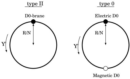
Figure 1: D0-branes

The identification with fractional D-branes can also be shown explicitly by examining the vacuum amplitude (3.28). By taking the orbifold limit, the summation part of NS-sector in (3.28) becomes

$$\lim_{R\rightarrow\infty}\sum_{l=0}^{N-1}\sum_{\alpha\in{\bf Z}}\exp\left[-\frac{\pi\alpha^{\prime}}{2R^{2}t}(N\alpha+l)^{2}+2\pi i\frac{k}{N}(N\alpha+l)\hat{J}\right],$$ (3.44)

$$= \!\!R\int^{\infty}_{-\infty}dp\ \exp{\left(-\frac{\pi\alpha^{\prime}N^{2}}{2t}p^{2}\right)}\sum^{N-1}_{l=0}\exp\left[2\pi i\frac{k}{N}l\hat{J}\right]\!\!=\!\!\frac{R}{2\pi\alpha^{\prime}}(8\pi^{2}\alpha^{\prime}t)^{\frac{1}{2}}\frac{\sum^{N-1}_{l=0}~{}g^{l}}{N}.$$

where $g=\exp[2\pi i\frac{k}{N}\hat{J}]$. Here we have used the fact that for NS-sector the eigenvalues of $\hat{J}$ take integers. On the other hand for R-sector $\hat{J}$ takes the half-integers, and the phase factor $\exp{(2\pi ik\alpha\hat{J})}=(-1)^{k\alpha}$ appears in the summation $\sum_{\alpha\in{\bf Z}}$. From this we can see that the amplitude in the R-sector becomes zero for odd $k$. Therefore the vacuum amplitude (3.28) under the orbifold limit becomes

$$\int^{\infty}_{0}\frac{dt}{2t}{\rm Tr}_{\scriptscriptstyle NS-R}\left[\frac{1+(-1)^{F}}{2}\frac{\sum^{N-1}_{l=0}~{}g^{l}}{N}~{}q^{H^{\prime}_{O}}\right] ~{}~{}(\mbox{for even}\ k),$$

$$\int^{\infty}_{0}\frac{dt}{2t}{\rm Tr}_{\scriptscriptstyle NS}\left[\frac{1+(-1)^{F}}{2}\frac{\sum^{N-1}_{l=0}~{}g^{l}}{N}~{}q^{H^{\prime}_{O}}\right] ~{}~{}(\mbox{for odd}\ k),$$ (3.45)

where $H^{\prime}_{O}=\alpha^{\prime}p^{2}+\hat{N}$ is the open string Hamiltonian. This is just the open string amplitude of a fractional D0-brane in type II for even $k$ and that in type 0 for odd $k$ (for fractional D-branes in type 0 theory see also [35]). In particular the absence of R-sector for the type 0 can be understood from the fact that there are no fermions on a type 0 D-brane, which can be verified by using the boundary state (3.43). Although the R-sector in type 0 can appear from the open strings between an electric D-brane and a magnetic D-brane, these two D-branes in (3.39) are infinitely far away from each other and its spectrum is neglected.

Let us return to the case of the finite radius $R$. From the above arguments the D-branes are expected to be similar to the fractional D0-branes in the orbifold theories. Indeed it is easy to see that the corresponding D0-branes are stuck at the point ($X^{\prime}$=$\bar{X}^{\prime}$=0) since there are no zero-modes of $X^{\prime},\bar{X}^{\prime}$ for non-integer $\gamma=\frac{\beta\alpha^{\prime}}{R}n=\frac{k}{N}n$ (see (2.1), (B)).

Up to now we have not considered the $U(1)$ phase in the coefficient $f_{\gamma}~{}(\ref{D0tension})$ of the boundary state (3.1). We can consider the freedom of the translation of D0-branes in the compactified $Y^{\prime}$ direction and this effect can be included in the boundary state (3.1) by replacing $f_{\gamma}$ with $f_{\gamma}\exp{(i\frac{n}{R}y^{\prime}_{0})}$ ($0\leq y^{\prime}_{0}<2\pi R$). To consider its meaning in the orbifold picture, where it is appropriate to regard the radius of ${\bf S^{1}}$ as $\frac{R}{N}$ (see Table.1 and eq.(3.39)), we reparametrize $y^{\prime}_{0}$ as $y^{\prime}_{0}=\tilde{y}^{\prime}_{0}+\frac{2\pi R}{N}a~{}(0\leq\tilde{y}^{\prime}_{0}<\frac{2\pi R}{N},~{}a=0,1,\cdots,N-1)$. Then its boundary state is written by

$$|B_{a},\epsilon\rangle_{\scriptscriptstyle NSNS,RR}=\sum_{n\in{\bf Z}}e^{i\frac{n}{R}\tilde{y}^{\prime}_{0}+2\pi i\frac{a}{N}n}|B,\gamma,\epsilon\rangle_{\scriptscriptstyle NSNS,RR}~{}~{}~{}~{}~{}~{}(\epsilon=\pm 1).$$ (3.46)

If we take the orbifold limit $R\rightarrow\infty$, the eq.(3.46) becomes the eq.(3.39) except that $\delta{(y^{\prime})}$ and $f^{\prime}_{l}$ are replaced by $\delta(y^{\prime}-\tilde{y}^{\prime}_{0})$ and $f^{\prime}_{l}\exp{(2\pi i\frac{a}{N}l)}$. Then if we remember that the fractional D-branes in an orbifold theory are labeled by irreducible representations of its discrete group [32, 33], we can see that these boundary states $(a=0,1\cdots N-1)$ represent the $N$ types of fractional D0-branes in the orbifold ${\bf C}/{\bf Z}_{N}$. Moreover, we can see that the translation of the D0-brane by $\frac{2\pi R}{N}$ in the $Y^{\prime}$ direction is equivalent to changing the types of the fractional D0-brane in the orbifold picture since this manipulation is equivalent to $a\rightarrow a+1$ in (3.46). This can be equally said that in the orbifold picture with the radius $\frac{R}{N}$ the $N$ types of fractional D0-branes are put at the same point $Y^{\prime}=\tilde{y}^{\prime}_{0}$, and receive the monodromy to change their types into each other if they go around ${\bf S^{1}}$ (see Fig.2).

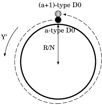
Figure 2: A fractional D0-brane receives the monodromy which changes its type.

This observation may be also supported by the mass spectrum of open strings between a $a$-type and a $b$-type D0-brane (we set $\tilde{y}^{\prime}_{0}=0$ for simplicity)

$$\alpha^{\prime}M^{2}=\frac{R^{2}}{N^{2}\alpha^{\prime}}\left(Nw-(k\hat{J}-a+b)\right)^{2}+\hat{N}.$$ (3.47)

For even $k$ the energy due to winding modes cannot vanish unless $a-b\in{\bf Z}$ and this shows that there are only $N$ types of D0-branes coincident at an arbitrary point in the orbifold picture. It would be useful if we could clarify the geometrical picture of the D0-brane in terms of the original coordinate $Y$, not the free field $Y^{\prime}$, of Melvin background (LABEL:SG1). This is complicated due to the T-duality transformations in section 2.1. We can speculate that the D0-brane, which is localized in the $Y^{\prime}$ direction, seems to be extended in the direction $Y$. This may be regarded as the $\rho=0$ limit of a torus-like D2-brane (see Fig.3) which we will discuss later.

For odd $k$ the energy for NS-sector due to winding modes in (3.47) can vanish for the appropriate values of $w,~{}a,~{}b$ and $\hat{J}$ (for example $w=a=b=\hat{J}=0$), while for R-sector it can not because $\hat{J}$ takes the half-integer values and there remains non-zero minimal energy $(\frac{R}{2N\alpha^{\prime}})^{2}$. This shows that a something like a bound system of an electric and a magnetic D0-brane exists in the Melvin background, being the finite distance $\frac{\pi R}{N}$ away from each other as we have already speculated from eq.(3.39). These interpretations of D0-branes are shown in Fig.1.

Finally we would like to mention the another orbifold limit $R\to 0$ with $qR=\frac{k}{N}$ and $\beta=0$. In this case we again obtain the orbifold ${\bf C}/{\bf Z}_{N}$. However, the boundary state (3.1) represents a bulk D0-brane in this orbifold limit since it depends only on $\beta$. Thus one may ask whether there exists a D0-brane for finite $R$ which is reduced to a fractional D0-brane in the limit $R\to 0$. Even though this is an intriguing problem, it will be beyond the scope of the present paper.

Bulk D0-branes

The fractional D0-branes are the most fundamental D0-branes in orbifold theories, and other D0-branes can be constructed by the linear combinations of them. In general these D0-branes can not leave from the fixed point $\rho=0$, while if we collect $N$ different types of fractional D0-branes they can move as an unit such that $\rho\neq 0$. The latter can be regarded as another type of the D0-brane in the orbifold theories which is called a bulk D0-brane, and it is known that the Chan-Paton bundle on this D0-brane obeys the regular representation for the discrete group ${\bf Z}_{N}$ [32].

Then it is natural to ask if such a D0-brane exists for the finite $R$. The answer is yes if the parameter $\frac{\beta\alpha^{\prime}}{R}$ is rational, and the bulk D0-brane in the Melvin background is defined as a bound state of $N$ different fractional D-branes whose positions are at $N$ different points $Y^{\prime}=0,\frac{2\pi R}{N},\cdot\cdot\cdot,\frac{2\pi R(N-1)}{N}$. Its boundary state is given by

$$|B_{bulk},\epsilon\rangle_{\scriptscriptstyle NSNS,RR} = \sum_{a=0}^{N-1}|B_{a},\epsilon\rangle_{\scriptscriptstyle NSNS,RR},$$ (3.48)

where $|B_{a},\epsilon\rangle_{\scriptscriptstyle NSNS,RR}$ is given by (3.46) (here we set $\tilde{y}^{\prime}_{0}=0$). The explicit form of the boundary state is obtained in the same way as (3.39) and the result is

$$\!\!|B_{bulk},\epsilon\rangle_{\scriptscriptstyle NSNS,RR}\!\!=\!\!\frac{T_{0}/2}{2(2\pi R/N)}\sum_{\alpha\in{\bf Z}}e^{i\frac{Ny^{\prime}}{R}\alpha}\left[|B,0,+\rangle_{\scriptscriptstyle\!\!NSNS,RR}-\!(-1)^{k\alpha}|B,0,-\rangle_{\scriptscriptstyle\!\!NSNS,RR}\right].$$ (3.49)

We can see that its boundary state is exactly the same form as that for a usual D-brane in type II string (for even $k$) or a bound system of an electric and a magnetic D-brane away from each other with $\frac{\pi R}{N}$ in type 0 string (for odd $k$) on ${\bf S^{1}}$ with finite $\frac{R}{N}$ (see Fig.1). Note that this boundary state does not have the twisted sectors $l\neq 0$ but picks up only the untwisted sector $l=0$ (or $n=N\alpha~{}(\alpha\in{\bf Z}$)). Thus the bosonic zeromodes $x_{0},\bar{x}_{0}$ indeed exist and the D0-brane can move around such that $\rho\neq 0$. To complete this argument one should also examine the first condition in eq.(3.6) carefully since the boundary state with $\rho\neq 0$ has a non-zero orbital angular momentum $\hat{J}_{0}$ in the zeromode part. Then the condition, which is equivalent to $(w-\frac{k}{N}\hat{J}_{0})|B\rangle=0$, is satisfied if $\hat{J}_{0}$ is a multiple of $N$. This requires that a bulk D-brane should consist of $N$ fractional D-branes which are located at the $N$ different points $X^{\prime}=\rho\ e^{i(\theta+2\pi ka/N)},\ \ (a=0,1,\cdot\cdot\cdot,N-1)$ on the plane, where $\theta$ is an arbitrary constant (see Fig.3). In this way we have shown that a bulk D0-brane exists if $\frac{\beta\alpha^{\prime}}{R}\in{\bf Q}$ for any values of parameters $q$ and $R$.

Next we consider its vacuum amplitude. The result is $N$ times as large as (3.25), while the second term of the open string Hamiltonian (3.26) is modified as follows

$$\left(\frac{R(w-k\hat{J})}{N\alpha^{\prime}}\right)^{2}\rightarrow\left\{\begin{array}[]{cc}(\frac{Rw}{N\alpha^{\prime}})^{2}{}&~{}(\mbox{for NS-sector and R-sector with even}~{}k),\\ \left(\frac{R(w+1/2)}{N\alpha^{\prime}}\right)^{2}{}&~{}(\mbox{for R-sector with odd}~{}k).\end{array}\right.$$ (3.51)

This is because the angular momentum operator $\hat{J}$ takes integer (half-integer) values in NS-sector (R-sector) and we can erase the effect of $\hat{J}$ by the shift of $w$. From this Hamiltonian we can see that there are no tachyonic modes though in the closed string sector there are in general. If we take the orbifold limit $R\rightarrow\infty$, the vacuum amplitude is $N$ times as large as (3.2) without the orbifold projection $\sum^{N-1}_{l=0}g^{l}/N$, which is the same as that in the flat type II theory for even $k$ or type 0 theory for odd $k$.

Finally we would also like to see how this D0-brane looks like in terms of the original Melvin coordinate $(X,\bar{X},Y)$. Remember that the coordinates $(X^{\prime},\bar{X}^{\prime},Y^{\prime})$ and $(X,\bar{X},Y)$ are related with each other by performing the T-duality twice as $\varphi^{\prime\prime}\to\tilde{\varphi}\to\varphi$ (see section 2.1). After the first T-duality procedure on $\varphi^{\prime\prime}$, the D0-brane located at $Y^{\prime}=\mbox{fixed},\ \rho=\mbox{fixed}(\neq 0)$ and $\varphi^{\prime\prime}=\mbox{fixed}$ will be changed into a D1-brane wrapped on the circle $0\leq\tilde{\varphi}<2\pi\alpha^{\prime}$. If we see this in terms of $(Y,\tilde{\varphi})$, the D1-brane can be viewed as a spiral D-string wrapped $N$ times on the circle $0\leq\tilde{\varphi}<2\pi\alpha^{\prime}$ and $k$ times on the circle $0\leq Y<2\pi R$ because of the relation $Y=Y^{\prime}-\beta\tilde{\varphi}$ in (2.5) . If we take the second T-duality on $\tilde{\varphi}$, then we obtain a D2-brane wrapped on the torus ${\bf T}^{2}\ni(Y,\varphi)$ (see Fig.3). This D2-brane should be regarded as a bound state of $k$ D2-branes and $N$ D0-branes as can be seen from the winding numbers of the spiral D-string. Note that this is consistent with the asymptotic value of $B$-field in (2.1) $B_{\varphi}=-\frac{1}{\beta}=-\frac{N\alpha^{\prime}}{kR}$ if $\beta\rho\gg 1$. From this value $B_{\varphi}$ we can show that if we consider the world-volume theory of a D2-brane on a torus ${\bf T}^{2}$ in the Seiberg-Witten limit [39], we will obtain the theory on a noncommutative torus with the noncommutativity parameter $\theta=\frac{k}{N}$.

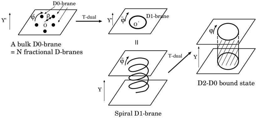
Figure 3: A bulk D0-brane can be regarded as a D2-D0 bound state in the Melvin background (2.1).

D1-branes Wrapped on ${\bf S}^{1}$

As we have seen, D0-branes in the Melvin background with the rational parameter are very similar to those in ${\bf Z}_{N}$ orbifolds. On the other hand, a D1-brane wrapped on ${\bf S}^{1}$ has an interesting structure which can not be explained clearly from the viewpoint of orbifold theories even though a D1-brane is formally transformed into a D0-brane by T-duality.

Here we consider the Melvin background with the rational parameter $qR=\frac{k}{N}$. The boundary state of a D1-brane can be constructed in the same way as that of a D0-brane. Then a single D1-brane is again pinned at the origin $\rho=0$ (fixed point) in (2.1). However if we consider $N$ D1-branes so that boundary state includes only the restricted winding sectors $w\in N{\bf Z}$, this bound system (‘bulk’ D1-brane) can move around in the plane ${\bf R^{2}}$ in the same way as in the previous case of D0-branes.

This behavior can be also explained geometrically as follows. Let us set $\beta=0$ for simplicity and assume that a single D1-brane is placed at $\rho\neq 0$. Though this D1-brane obeys the Dirichlet boundary condition along $(X^{\prime},\bar{X}^{\prime})\in{\bf R}^{2}$, in the original coordinate $(X,\bar{X})$ it is rotated by the angle $\frac{2\pi k}{N}$ if it goes around ${\bf S}^{1}$ once, as shown in eq.(2.11). Thus it should wind $N$ times around ${\bf S}^{1}$ in order to move around on the ${\bf R^{2}}$ plane (see Fig.4). It is also useful to note that the geodesic lines along ${\bf S}^{1}$ are given by $\varphi+qy=\mbox{constant}$ from (2.2) and agrees with the world-volume of the D1-brane. This is a good tendency since it will minimize the mass of the D-brane.

The analysis of the orbifold limit $R\to 0$ with $qR=\frac{k}{N}$ and $\frac{\beta\alpha^{\prime}}{R}\to 0$ can be performed in the same way as before. A single D1-brane (below we reuse the coordinate $(X^{\prime},\bar{X}^{\prime},Y^{\prime})$) which is sticked at the fixed point is identical to a fractional D0-brane in the limit by T-duality. On the other hand, the D1-brane winding $N$ times around ${\bf S}^{1}$ corresponds to a bulk D0-brane which is made of $N$ fractional D0-branes in the orbifold ${\bf C}/{\bf Z}_{N}$.

Let us consider the vacuum amplitude for a ‘bulk’ D1-brane. The momentum part of the open string Hamiltonian (the T-dual picture of (3.26)) is given by

$$\left(\frac{n-k\hat{J}}{NR}\right)^{2}\rightarrow\left\{\begin{array}[]{cc}(\frac{n}{NR})^{2}{}&~{}(\mbox{for NS-sector and R-sector with even}~{}k),\\ (\frac{n+1/2}{NR})^{2}{}&~{}(\mbox{for R-sector with odd}~{}k).\end{array}\right.$$ (3.53)

Note that for odd $k$ case the obtained D1-brane is really a system which consists of an electric ‘bulk’ D1-brane and a magnetic ‘bulk’ D1-brane. They wind $N$ times around ${\bf S}^{1}$ and there is also a ${\bf Z}_{2}$ Wilson line on either D1-brane.

In this way we have found that a D1-brane wrapped on ${\bf S}^{1}$ in the Melvin background has the spiral structure (see Fig.4). As can be seen from the open string Hamiltonian there are again no tachyonic modes even though in the closed string sector there are tachyons in general.

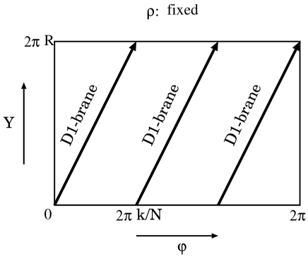
Figure 4: Spiral D1-branes

Other Dp-branes

The analysis of other D-branes can be done in the same way. We have only to consider the three dimensional Melvin geometry out of the ten dimensional spacetime. Then both a D3-brane and a D2-brane which are extended in the $X^{\prime},\bar{X}^{\prime}$ directions are also allowed (see the Table.1). Each of these becomes a ‘fractional’ D2-brane on the space ${\bf C}/{\bf Z}_{N}$ in the orbifold limit (for D3-branes we take a T-duality transformation in the $Y^{\prime}$ direction). This kind of D2-brane has the same tension as an ordinary D2-brane in almost the same way as in orbifold theories [63].

For the rational case there exists another D-brane which obeys the Neumann-Dirichlet or Dirichlet-Neumann boundary conditions for $X^{\prime},\bar{X}^{\prime}$ directions as we mentioned below (3.16). For bulk D-branes we can define such boundary conditions because on such D-branes the parameter $\gamma$ which appears in the boundary states takes an integer value. Especially note that these D-branes can not be defined as bound systems of $N$ kinds of fractional D-branes such as (3.48).

Such an example also appears for $\frac{\beta\alpha^{\prime}}{R}=\frac{k}{N}$ (or $qR=\frac{k}{N}$) with even $N$ and odd $k$. In this background we can consider a D-brane with the untwisted sector $\hat{\gamma}=0$ and one twisted sector $\hat{\gamma}=\frac{1}{2}$, which is just the condition to allow the mixed boundary conditions (see below (3.16)).

Here we have obtained the several D-branes in Melvin background, thus we summarize these results in the Table 2.

$Y^{\prime}$	$X^{\prime},\bar{X}^{\prime}$	Existence	Mobility	Tension	Form	Orbifold Limit
D	DD	all	Pinned	$T_{0}$	a D0-brane	fractional D0
D	DD	$\frac{\beta\alpha^{\prime}}{R}=\frac{k}{N}$	Movable	$NT_{0}$	$N$ D0-branes	bulk D0
D	DN	$\frac{\beta\alpha^{\prime}}{R}=\frac{k}{N}$	Movable	$NT_{1}$	$N$ D1-branes	bulk D1
D	NN	all	—	$T_{2}$	a D2-brane	‘fractional’ D2
N	DD	all	Pinned	$T_{1}$	a D1-brane	fractional D0
N	DD	$qR=\frac{k}{N}$	Movable	$NT_{1}$	$N$ spiral D1-branes	bulk D0
N	DN	$qR=\frac{k}{N}$	Movable	$NT_{2}$	$N$ spiral D2-branes	bulk D1
N	NN	all	—	$T_{3}$	a D3-brane	‘fractional’ D2

Table 2: D-brane spectrum in the Melvin background. Here we define the boundary condition of open strings in terms of free fields $(X^{\prime},\bar{X}^{\prime},Y^{\prime})$. Note that for odd $k$ we regard a D$p$ in the above as a bound state of an electric D$p$ and a magnetic D$p$.

3.3 Structure of D-branes for the Irrational Parameters

As we have already mentioned, the D-brane spectrum for the irrational parameters is remarkably different from the previous case of rational parameters. A single D-brane can exist only at the origin $\rho=0$ in (2) as before. However if one wants to put D-branes at the other points $\rho\neq 0$, then one must prepare infinitely many D-branes, which can be verified by calculating its tension in the same way as before. This fact matches the intuitive picture of the irrational case as a large $N$ limit of the orbifold ${\bf C}/{\bf Z}_{N}$ [13]. For example, let us consider a D1-brane wrapped on ${\bf S}^{1}$. In the irrational case the D1-brane along the geodesic line cannot return to the original point even if it goes around ${\bf S}^{1}$ any times. Thus the system will be a sort of a ‘foliation’ of the cylinder $\rho=\mbox{constant}$ and may be like a 2-brane. Even though we cannot answer whether such a system can really exist, we can say that the D-brane spectrum for the irrational case is more restricted than that for the rational case.

3.4 World-Volume Theory

In the above we have constructed boundary states of various D-branes and have seen their geometric interpretations. Here we would like to briefly discuss the world-volume theory on these D-branes.

First note that the boundary states which have the Neumann (or Dirichlet) boundary condition in the $Y^{\prime}$ direction depend only on the parameter $qR$ (or $\frac{\beta\alpha^{\prime}}{R}$) and not on another. This fact is the reason why a D-brane in the background where one of the parameters is rational is treated as if it was a fractional D-brane, even though another parameter is irrational and this background is not equivalent to any freely acting orbifolds.

This fact will also lead to the intriguing property that the mass spectrum of open string which obeys the Dirichlet boundary condition along ${\bf S}^{1}$ can show the Bose-Fermi degeneracy for $\beta=0$ and $q\neq 0$ even if the supersymmetry is completely broken in the closed string sector. This mysterious phenomenon can be a relic of the supersymmetry in type II theory, which is spontaneously broken [51] by the non-zero value of $q$. In other words the Bose-Fermi degeneracy only on the point-like D-brane along ${\bf S}^{1}$ implies the remained local supersymmetry, while the degeneracy does not occur on the D-brane wrapped on ${\bf S}^{1}$ because of the lack of global supersymmetry.

Next let us consider the relation to the quiver gauge theory [32]. In particular we take a D0-brane as an example. Let us remember the open string mass spectrum (3.47). If we take the orbifold limit $R\to\infty$, then it is easy to see that the ${\bf Z}_{N}$ projection of quiver theory

$$k\hat{J}-a+b=Nw\in N{\bf Z},$$ (3.54)

appears, which restricts the spectrum to $g~{}(=\exp{[2\pi i\frac{k}{N}\hat{J}]})=\exp{[2\pi i\frac{a-b}{N}]}$. Thus the world-volume theory on D0-branes in the Melvin background can be regarded as a deformation of the quiver theory whose ${\bf Z}_{N}$ projection is softened. One can also see that the opposite limit $R\to 0$ leads to the mass spectrum of an ordinary D0-brane in type II theory. Thus for a finite radius the world-volume theory is regarded as an interpolation between them. In particular the massless fields are the same as those of the quiver gauge theory of the orbifold ${\bf C/Z}_{N}$.

4 D-branes in Supersymmetric Higher Dimensional Models

The closed string backgrounds we have discussed above do not preserve any supersymmetry in general. If we would like to discuss D-brane charges, it will be more desirable to consider those in supersymmetric backgrounds. Therefore in this section we investigate D-branes in the higher dimensional generalization of the Melvin model [13, 14], which includes the supersymmetric background. This model has a background of the form $\mbox{ \bf M}_{5}\times{\bf R}^{1,4}$, where $\mbox{\bf M}_{5}$ is a ${\bf S}^{1}\ni Y$ fibration over ${\bf R}^{2}\times{\bf R}^{2}\ni(X^{1},\bar{X}^{1},X^{2},\bar{X}^{2})$. Correspondingly this model has four magnetic parameters $q_{1},q_{2},\beta_{1}$ and $\beta_{2}$, and the explicit metric of this model is given in the paper [13]. The four of eight (light-cone gauge) spinor fields in the Green-Schwarz formulation do not suffer from the phase factor when $\sigma$ is shifted by $2\pi$ iff $q_{1}=q_{2},\beta_{1}=\beta_{2}$ or $q_{1}=-q_{2},\beta_{1}=-\beta_{2}$. Therefore we can conclude that in these specific cases half of thirty two supersymmetries will be preserved. Indeed we can also show that the partition function does vanish for these cases [13]. From the supergravity viewpoint, we can see this as follows. For simplicity, let us set $\beta_{1}=\beta_{2}=0$. Then if the spinor fields go around the circle ${\bf S}^{1}$, they obtain the phase $e^{i\pi(\pm q_{1}\pm q_{2})R}$. Thus if $q_{1}=q_{2}$ or $q_{1}=-q_{2}$, there are sixteen Killing spinors. This special case $q_{1}=\pm q_{2},\beta_{1}=\beta_{2}=0$ can be regarded as the ‘$9-11$’ flip of the supersymmetric F5-brane [21]. We would also like to mention that similar arguments can also be generalized into much higher dimensional backgrounds $\mbox{\bf M}_{7}$ (F3-brane), $\mbox{\bf M}_{9}$ (F1-brane) [13, 14]. The results on the behavior of D-branes discussed below will also be applied to these more generalized cases without any serious modifications.

4.1 Sigma Model Description and Mass Spectrum

If we consider the higher dimensional generalizations of (LABEL:SG1) its world-sheet action is given as follows :

$$S = \frac{1}{\pi\alpha^{\prime}}\int d^{2}\sigma\Bigl{[}\bar{\partial}\rho\partial\rho+\bar{\partial}r\partial r+\rho^{2}\bar{\partial}\check{\varphi}\partial\check{\varphi}+r^{2}\bar{\partial}\check{\theta}\partial\check{\theta}$$ (4.1)

$$+(1+\beta_{1}^{2}\rho^{2}+\beta_{2}^{2}r^{2})^{-1}(\bar{\partial}Y+\beta_{1}\rho^{2}\bar{\partial}\check{\varphi}+\beta_{2}r^{2}\bar{\partial}\check{\theta})(\partial Y-\beta_{1}\rho^{2}\partial\check{\varphi}-\beta_{2}r^{2}\partial\check{\theta})\Bigr{]},$$

where we have defined $\check{\varphi}=\varphi+q_{1}Y,\ \check{\theta}=\theta+q_{2}Y$. After T-duality of $Y$ into $\tilde{Y^{\prime}}$, we obtain

$$S=\frac{1}{\pi\alpha^{\prime}}\int d^{2}\sigma\left[\bar{\partial}\rho\partial\rho+\bar{\partial}r\partial r+\bar{\partial}\tilde{Y^{\prime}}\partial\tilde{Y^{\prime}}+\rho^{2}\bar{\partial}\varphi^{\prime\prime}\partial\varphi^{\prime\prime}+r^{2}\bar{\partial}\theta^{\prime\prime}\partial\theta^{\prime\prime}\right],$$ (4.2)

where $\varphi^{\prime\prime}\equiv\check{\varphi}-\beta_{1}\tilde{Y^{\prime}},\ \ \theta^{\prime\prime}\equiv\check{\theta}-\beta_{2}\tilde{Y^{\prime}}$ are the higher dimensional generalization of $\varphi^{\prime\prime}$ which appeared in eq.(2.9). The T-dual of $\tilde{Y^{\prime}}$ is equivalent to $Y^{\prime}$ in eq.(2.6). The zero-mode of $Y^{\prime}$ is quantized in the same way as (2.19)

$$P^{\prime}_{L}+P^{\prime}_{R}=2\left(\frac{n}{R}-q_{1}\hat{J}_{1}-q_{2}\hat{J}_{2}\right),\ \ \ P^{\prime}_{L}-P^{\prime}_{R}=2\left(\frac{Rw}{\alpha^{\prime}}-\beta_{1}\hat{J}_{1}-\beta_{2}\hat{J}_{2}\right),$$ (4.3)

where the angular momenta $\hat{J}_{1}=\hat{J}_{1L}+\hat{J}_{1R}$ and $\hat{J}_{2}=\hat{J}_{2L}+\hat{J}_{2R}$ are defined for each ${\bf R}^{2}$ as were done in eq.(2.14).

From (4.2) the bosonic fields $X^{1^{\prime}}\!=\!\rho e^{i\varphi^{\prime\prime}},\ \ X^{2^{\prime}}\!=\!re^{i\theta^{\prime\prime}}$ and their superpartners $\psi^{1^{\prime}}_{L},\psi^{1^{\prime}}_{R},\psi^{2^{\prime}}_{L},\psi^{2^{\prime}}_{R}$ become free fields and they obey the following boundary conditions for each $i=1,2$

$$X^{i^{\prime}}(\tau,\sigma+2\pi) = e^{2\pi i\gamma_{i}}X^{i^{\prime}}(\tau,\sigma),$$

$$\psi^{i^{\prime}}_{L}(\tau,\sigma+2\pi) = e^{2\pi i\gamma_{i}}\psi^{i^{\prime}}_{L}(\tau,\sigma),\ \ \ \ \psi^{i^{\prime}}_{R}(\tau,\sigma+2\pi)=e^{2\pi i\gamma_{i}}\psi^{i^{\prime}}_{R}(\tau,\sigma),$$ (4.4)

where $$\hat{\gamma_{i}}\equiv\gamma_{i}-[\gamma_{i}],\ \ \ \gamma_{i}\equiv q_{i}Rw+\beta_{i}\alpha^{\prime}(\frac{n}{R}-q_{1}\hat{J}_{1}-q_{2}\hat{J}_{2}).$$ (4.5)

Then we can obtain the mass spectrum as follows

$$\frac{\alpha^{\prime}M^{2}}{2} = \frac{\alpha^{\prime}}{2R^{2}}(n-q_{1}R\hat{J}_{1}-q_{2}R\hat{J}_{2})^{2}+\frac{R^{2}}{2\alpha^{\prime}}(w-\frac{\alpha^{\prime}}{R}\beta_{1}\hat{J}_{1}-\frac{\alpha^{\prime}}{R}\beta_{2}\hat{J}_{2})^{2}$$ (4.6)

$$+\hat{N}_{R}+\hat{N}_{L}-\sum_{i=1}^{2}\hat{\gamma_{i}}(\hat{J}_{Ri}-\hat{J}_{Li}),$$

with the level matching constraint

$$\hat{N}_{R}-\hat{N}_{L}-nw+\sum_{i=1}^{2}[\gamma_{i}]\hat{J}_{i}=0,$$ (4.7)

where $\hat{N}_{L,R}$ is defined in the same way as (B). From the above expression we can find the T-duality symmetry $q_{i}\leftrightarrow\beta_{i},~{}R\leftrightarrow\frac{\alpha^{\prime}}{R}$ if $q_{1}\beta_{2}=q_{2}\beta_{1}$. Note that the supersymmetric model ($q_{1}=\pm q_{2}$, $\beta_{1}=\pm\beta_{2}$) satisfies this condition.

It is also easy to see that if $n_{1}+n_{2},\ n_{1}-n_{2}\in 2{\bf Z}$, we obtain the following periodicity

$$Z(R,q_{1},q_{2},\beta_{1},\beta_{2})=Z(R,q_{1}+\frac{n_{1}}{R},q_{2}+\frac{n_{2}}{R},\beta_{1},\beta_{2}),$$ (4.8)

and the periodicity for $\beta_{i}$ can be also obtained by the T-duality.

4.2 Supersymmetric D-branes

We can consider D-branes in the higher dimensional Melvin model in the same way as in section three. The quantization of open strings can be performed because the action is already rewritten by free fields and we can construct the boundary states of D-branes. Its explicit form is almost the same as in eq.(3.1) and eq.(3.1). By using such boundary states we can obtain the vacuum amplitude, for example, for a D0-brane as follows

$$A = \frac{\pi\alpha^{\prime}V_{0}}{8\pi R}\int^{\infty}_{0}\frac{dt}{t^{2}}$$ (4.9)

$$\times\Biggl{[}\Bigl{\{}\sum_{\gamma_{1}\in{\bf Z},\gamma_{2}\in{\bf Z}}\frac{|f_{\gamma}|^{2}}{(2\pi^{2}\alpha^{\prime})^{4}}(\eta(it))^{-12}+\sum_{\gamma_{1}\notin{\bf Z},\gamma_{2}\in{\bf Z}}\frac{(-1)^{[\gamma_{1}]}|f_{\gamma}|^{2}}{(2\pi^{2}\alpha^{\prime})^{3}}(\eta(it))^{-9}(\theta_{1}(\gamma_{1}|it))^{-1}$$

$$~{}~{}~{}~{}~{}~{}~{}~{}~{}~{}~{}~{}~{}~{}~{}+\sum_{\gamma_{1}\in{\bf Z},\gamma_{2}\notin{\bf Z}}\frac{(-1)^{[\gamma_{2}]}|f_{\gamma}|^{2}}{(2\pi^{2}\alpha^{\prime})^{3}}(\eta(it))^{-9}(\theta_{1}(\gamma_{2}|it))^{-1}$$

$$~{}~{}~{}~{}~{}~{}~{}~{}~{}~{}~{}~{}~{}~{}~{}+\sum_{\gamma_{1}\notin{\bf Z},\gamma_{2}\notin{\bf Z}}\frac{(-1)^{[\gamma_{1}]+[\gamma_{2}]}|f_{\gamma}|^{2}}{(2\pi^{2}\alpha^{\prime})^{2}}(\eta(it))^{-6}(\theta_{1}(\gamma_{1}|it))^{-1}(\theta_{1}(\gamma_{2}|it))^{-1}\Bigr{\}}$$

$$~{}~{}~{}~{}~{}~{}~{}~{}~{}~{}~{}~{}~{}~{}~{}~{}~{}~{}~{}~{}\times\exp\left(-\frac{\pi\alpha^{\prime}}{2R^{2}t}n^{2}\right)(\theta_{1}(\frac{\gamma_{1}+\gamma_{2}}{2}|it))^{2}(\theta_{1}(\frac{\gamma_{1}-\gamma_{2}}{2}|it))^{2}\Biggr{]},$$

where $\gamma_{i}=\frac{\beta_{i}\alpha^{\prime}}{R}n$, and the summations should be performed about $n\in{\bf Z}$ such that the conditions indicated below the symbol $\sum$ are satisfied. Note also that we have transformed the result obtained in the NS-R formulation into that in the Green-Schwarz formulation using the formula (C.4).

Such vacuum amplitude should be consistent with the Cardy’s condition and this determines the coefficient $f_{\gamma}$ which appears as in eq.(3.1). The result for a general Dp-brane is given by

$$f_{\gamma}=\left\{\begin{array}[]{cc}\frac{1}{2}T_{p}{}&~{}(\gamma_{1}\in{\bf Z},\gamma_{2}\in{\bf Z}),\\ \frac{1}{\sqrt{2}}(\frac{|\sin{\pi\gamma_{1}}|}{2\pi^{2}\alpha^{\prime}})^{\mp\frac{1}{2}}T_{p}{}&~{}(\gamma_{1}\notin{\bf Z},\gamma_{2}\in{\bf Z}),\\ \frac{1}{\sqrt{2}}(\frac{|\sin{\pi\gamma_{2}}|}{2\pi^{2}\alpha^{\prime}})^{\mp\frac{1}{2}}T_{p}{}&~{}(\gamma_{1}\in{\bf Z},\gamma_{2}\notin{\bf Z}),\\ (\frac{|\sin{\pi\gamma_{1}}|}{2\pi^{2}\alpha^{\prime}})^{\mp\frac{1}{2}}(\frac{|\sin{\pi\gamma_{2}}|}{2\pi^{2}\alpha^{\prime}})^{\mp\frac{1}{2}}T_{p}{}&~{}(\gamma_{1}\notin{\bf Z},\gamma_{2}\notin{\bf Z}),\end{array}\right.$$ (4.14)

where the sign factor $\mp$ in the exponent of $|\sin\pi\gamma_{i}|~{}(i=1,2)$ takes $-$ for D-branes with Neumann-Neumann boundary condition, $+$ for D-branes with Dirichlet-Dirichlet boundary conditions for $X^{i^{\prime}},\bar{X}^{i^{\prime}}$ directions. In the Neumann-Dirichlet case one can define the boundary state in the same way only if $\gamma$ is an integer or a half-integer. The above result (4.14) shows that a Dp-brane in the background has the ordinary tension $T_{p}$.

The structures of these D-branes are almost similar to those in the original Melvin background discussed in section 3. However we notice a remarkable property in this case: under the condition that the supersymmetry in the closed string theory is preserved ($\beta_{1}=\pm\beta_{2}$ and $q_{1}=\pm q_{2}$) the open string one-loop amplitude (4.9) vanishes. Thus the D-branes in this special background are stable BPS objects. In the orbifold limit $R\to\infty$ with

$$\frac{\beta_{1}\alpha^{\prime}}{R}=\pm\frac{\beta_{2}\alpha^{\prime}}{R}=\frac{k}{N},\ \ \ q_{1}=q_{2}=0,$$ (4.15)

these D-branes are identified with BPS fractional D-branes [32, 33] in the supersymmetric ALE orbifolds ${\bf C}^{2}/{\bf Z}_{N}$. More generally, if $\frac{\beta_{i}\alpha^{\prime}}{R}=\frac{k_{i}}{N}~{}(i=1,2)$ and if $k_{1}+k_{2}$ is even, the D-brane in the limits becomes a fractional D-brane in type II (not necessarily supersymmetric) orbifolds ${\bf C}^{2}/{\bf Z}_{N}$. On the other hand, if $k_{1}+k_{2}$ is odd, it is divided into an electric and a magnetic fractional D-brane [35] in type 0 orbifolds ${\bf C}^{2}/{\bf Z}_{N}$.

According to the parameter values $q_{i}R$ and $\frac{\beta_{i}\alpha^{\prime}}{R}$ $(i=1,2)$ the D-brane spectrum dramatically changes again. For the irrational values only the D-branes which are stuck at the fixed point are allowed, while for the rational values there also exist the D-branes which can move around. The latter are made of $N$ ‘fractional’ D-branes, which can be seen as a generalization of a bulk D-brane in the orbifold theory ${\bf C}^{2}/{\bf Z}_{N}$ [32]. The detailed arguments of these D-branes are almost the same as before.

4.3 Comments on D-brane Charges and K-theory

Before we conclude this paper, let us briefly mention the D-brane charges in the supersymmetric Melvin background. It is known that D-brane charges in type IIB and IIA theory are generally classified by K-theory $K^{0}(X)$ and $K^{1}(X)$ [44, 65], where $X$ represents the manifold of the spacetime considered. First we assume that the parameters are given by (4.15). Then it is easy to see that the number of massless RR-fields are given by one for finite $R$ and by $N$ for the orbifold limit $R\to\infty$. In the orbifold language each of these $N$ RR-fields comes from one untwisted sector and $N-1$ twisted sectors. Naively one may think that the number of types of D$p$-branes should be given by $N$ in accordance with the $N$-types of boundary states (3.46). However one should remember that for finite $R$ the type of a fractional D-brane changes if it goes around the compactified circle. This shows that the types of fractional D-branes (twisted RR-charge) do not preserve unless we take the limit $R\to\infty$. Thus we conclude that the D-brane charge or equally the corresponding K-group should be given by the rather trivial result $K^{0}(M_{5})=K^{1}(M_{5})={\bf Z}$ for finite $R$. On the other hand if we take the orbifold limit $R\to\infty$, then the K-group should be given by the equivalent K-theory $K^{0}_{{\bf Z}_{N}}({\bf R}^{4})={\bf Z}^{N}$ [44, 65], which corresponds to the $N$-types of fractional D-branes on the orbifold ${\bf C}^{2}/{\bf Z}_{N}$. Thus the spectrum of D-brane charges does not appear to be continuously connected in the orbifold limit even though the masses of twisted RR-fields which couple D-branes continuously change. It would be interesting for the above facts to be understood from the viewpoint of the K-theory with $H$-flux like the twisted K-theory $K_{H}(X)$ discussed in [45, 46].

Next we would like to consider the case where $\frac{\beta_{i}\alpha^{\prime}}{R}$ is irrational with $q_{1}=q_{2}=0$. Then we find that in the limit $R\rightarrow\infty$ (a ‘large $N$ limit of the orbifold’ [13]) there seems to be infinitely many massless RR-fields absorbing the zeromode along the circle ${\bf S}^{1}$. Thus we may have the ‘K-group’ $K^{0}(M_{5})=K^{1}(M_{5})={\bf Z}^{\infty}$ in this limit even though for the irrational parameters the space $M_{5}$ is no longer a smooth manifold nor a ‘good’ singular manifold like ordinary orbifolds.

It may not be so nonsense even to ask whether one can explain D-brane charges in type 0 theory from the viewpoint of K-theory if one remembers that the type II Melvin background approaches type 0 theories with the appropriate limits.

5 Conclusions and Discussions

In this paper we have investigated various aspects of D-branes in Melvin backgrounds by employing the boundary state formalism. The boundary states are constructed in terms of the free field representations which can be obtained by applying T-duality to the original sigma model of the Melvin backgrounds. Then we can impose the ordinary Neumann or Dirichlet boundary conditions on the free fields, though the resulting D-branes are geometrically non-trivial in the Melvin backgrounds.

The D-brane spectrum turns out to depend sensitively on whether the magnetic parameters $qR$ and $\frac{\beta\alpha^{\prime}}{R}$ are rational or irrational. In the former case the boundary states have the structure similar to orbifold theories and indeed they become the fractional D-branes in the orbifolds ${\bf C}^{n}/{\bf Z}_{N}$ if we take the large radius (or small radius in T-dual picture) limits. For finite radius the $N$ kinds of ‘fractional D-branes’ which belong to the different irreducible representations of ${\bf Z}_{N}$ can be changed into each other by the monodromy if they go around the compactified circle. Even though a single (‘fractional’) D-brane cannot move away from the fixed point (or the origin), $N$ different kinds of ‘fractional’ D-branes can move around as a unit (a ‘bulk’ D-brane). On the other hand, in the case of irrational parameters one needs the infinite number of the ‘fractional’ D-branes in order to move away from the fixed point. We left the possibility of the existence of such D-branes as an unresolved problem.

The orbifold theory we obtain in the limits is defined in either type 0 or type II string theory depending on the rational parameters. In the type 0 case we found that a D-brane behaves like a combined system of an electric fractional D-brane and a magnetic fractional D-brane.

The individual effects of two parameters $q$ and $\beta$ are roughly as follows. The non-zero value of the parameter $q$ twists the plane ${\bf R}^{2}$ spirally along the circle ${\bf S}^{1}$. As a result the world-volume of a D-brane which wraps the circle is bended along a spiral geodesic line (see eq.(2.2)). The effect of non-zero $\beta$, which means the non-zero $H$-flux, is more complicated because one should mix the free fields with its T-dualized ones as in eq.(2.5) and (2.11) in order to return back to the original Melvin sigma model (LABEL:SG1). This complexity may be due to the presence of $H$-flux. Owing to this T-duality transformation, a bulk D0-brane at $\rho\neq 0$ in terms of the free fields $(X^{\prime},\bar{X}^{\prime},Y^{\prime})$ is interpreted as a D2-D0 bound state which wraps the two dimensional torus ($\rho=\mbox{fixed}$) in the original Melvin background (2.1). Interestingly, this two dimensional torus can be regarded as a non-commutative torus $\mathcal{A}_{\theta}$ with the noncommutativity $\theta=\frac{\beta\alpha^{\prime}}{R}$ if we assume that the $B$-field is large $\beta\rho\gg 1$ and apply the argument in [39]. The observed dependence of D-branes on the parameters can be now reinterpreted as that on the parameter of the non-commutative torus $\mathcal{A}_{\theta}$. The corresponding operator algebra K-theory $K(\mathcal{A}_{\theta})={\bf Z}+\theta{\bf Z}$ [66] shows the analogous difference between the rational and the irrational case, where the value ${\bf Z}+\theta{\bf Z}(\in{\bf R})$ means the dimension of the corresponding projective module. Indeed two ${\bf Z}$ charges in the K-group $K(\mathcal{A}_{\theta})$ represent the D2-brane and the D0-brane charges as is clearly explained from the viewpoint of the tachyon condensation in the open string theory [67]. It would be interesting to examine the noncommutative algebra on such D-branes by using the free field calculations since this background possesses non-zero $H$-flux (for a general discussion on the relation between $H$-flux and noncommutative geometry see [40]).

Such an interpretation of a D0-brane in the free field model (2.6) as a D2-D0 bound state in the Melvin sigma model (LABEL:SG1) seems to raise some intriguing questions. The first question is whether an ordinary D0-brane can also exist in the Melvin background (2.1) and what is the form of its boundary state if it exists. The second is why such a D2-D0 bound state can exist in the Melvin background which does not wrap any homologically non-trivial cycle. We leave these issues as future problems.

It is also an interesting result that the boundary states of D-branes depend only on either of two parameters. This phenomenon leads to the strange Bose-Fermi degeneracy on specific D-branes even in nonsupersymmetric string backgrounds. We pointed out the interpretation of this as a remnant of the spontaneously broken supersymmetry.

Finally we would like to note that we can apply the above results for the original Melvin background (2.1) to its higher dimensional generalizations without any serious modifications as we have seen in section 4. For specific values of parameters the model preserves some supersymmetries and the D-branes there become BPS states. Thus it would be interesting to explore their supersymmetric world-volume theories and their statuses from the viewpoint of the string dualities.

Acknowledgments

We are grateful to Y. Hikida, K. Ichikawa, H. Kajiura and E. Ogasa for useful discussions. T.T. is supported by JSPS Research Fellowships for Young Scientists.

Note Added

After completing this paper we noticed the paper [68] on the net, which has some overlaps with our paper.

Appendix A T-duality for Kaluza-Klein Background

The coordinate of world-sheet is $z=\sigma_{1}+i\sigma_{2}$ and we define its partial derivative as $\partial=\frac{1}{2}(\partial_{1}-i\partial_{2}),\bar{\partial}=\frac{1}{2}(\partial_{1}+i\partial_{2})$. Let us first consider the following bosonic sigma model:

$$S=\frac{1}{\pi\alpha^{\prime}}\int d^{2}\sigma\left[(G_{ij}(X)+B_{ij}(X))\partial X^{i}\bar{\partial}X^{j}+\frac{1}{4}\alpha^{\prime}R^{(2)}\phi(X)\right].$$ (A.1)

After substituting the Kaluza-Klein background like (2.1) we obtain

$$S = \frac{1}{\pi\alpha^{\prime}}\int d^{2}\sigma\Bigl{[}(G_{\mu\nu}(X)+B_{\mu\nu}(X))\bar{\partial}X^{\nu}\partial X^{\mu}+e^{2\sigma(X)}(\bar{\partial}Y+A_{\mu}\bar{\partial}X^{\mu})(\partial Y+A_{\mu}\partial X^{\mu})$$ (A.2)

$$\ \ \ \ \ \ \ \ \ \ \ +B_{\mu}(\bar{\partial}Y\partial X^{\mu}-\bar{\partial}X^{\mu}\partial Y)+\frac{1}{4}\alpha^{\prime}R^{(2)}\phi(X)\Bigr{]}.$$

Then we can perform T-duality along $Y$ direction (${\bf S^{1}}$ with radius $R$) since the fields $G_{\mu\nu}(X),B_{\mu\nu}(X),\phi(X)$ do not depend on $Y$ [50]. Introducing the auxiliary vector field $V,\bar{V}$ we can rewrite (A.2) as follows (we show only nontrivial parts)

$$S = \frac{1}{\pi\alpha^{\prime}}\int d^{2}\sigma\Bigl{[}e^{2\sigma(X)}(\bar{V}+A_{\mu}\bar{\partial}X^{\mu})(V+A_{\mu}\partial X^{\mu})+B_{\mu}(\bar{V}\partial X^{\mu}-\bar{\partial}X^{\mu}V)$$ (A.3)

$$\ \ \ \ \ \ \ \ \ \ \ \ +(\bar{V}\partial\tilde{Y}-\bar{\partial}\tilde{Y}V)\Bigr{]},$$

where the new field $\tilde{Y}$ is compactified on a circle with the radius $\frac{\alpha^{\prime}}{R}$. If we first integrate $\tilde{Y}$, then we obtain $\bar{\partial}V-\partial\bar{V}=0$ and the vector field $V,\bar{V}$ can be written as $V=\partial Y,\ \bar{V}=\bar{\partial}Y$. Indeed one can easily see that this field $Y$ has the periodicity $Y\sim Y+2\pi R$ as expected. Next it is straightforward to integrate out $V$ first and one obtains

$$S = \frac{1}{\pi\alpha^{\prime}}\int d^{2}\sigma\Bigl{[}\cdot\cdot\cdot+e^{-2\sigma(X)}(\bar{\partial}\tilde{Y}+B_{\mu}\bar{\partial}X^{\mu})(\partial\tilde{Y}+B_{\mu}\partial X^{\mu})+A_{\mu}(\bar{\partial}\tilde{Y}\partial X^{\mu}-\bar{\partial}X^{\mu}\partial\tilde{Y})$$ (A.4)

$$\ \ \ \ \ \ \ \ \ \ \ \ +\frac{1}{4}\alpha^{\prime}R^{(2)}(\phi(X)-\sigma(X))\Bigr{]},$$

where the shift of the dilaton field can be determined from the condition of the conformal invariance (vanishing beta-function) [50]. Thus we have obtained the following T-duality transformation:

$$\sigma^{\prime}(X)=-\sigma(X),\ \ A_{\mu}^{\prime}(X)=B_{\mu}(X),\ \ B_{\mu}^{\prime}(X)=A_{\mu}(X),\ \phi^{\prime}(X)=\phi(X)-\sigma(X).$$ (A.5)

Note also that the equation of motion of (A.2) is equivalent to that of (A.4) via the rule:

$$\partial\tilde{Y} = -B_{\mu}\partial X^{\mu}-e^{2\sigma}(\partial Y+A_{\mu}\partial X^{\mu}),$$

$$\bar{\partial}\tilde{Y} = -B_{\mu}\bar{\partial}X^{\mu}+e^{2\sigma}(\bar{\partial}Y+A_{\mu}\bar{\partial}X^{\mu}).$$ (A.6)

In this paper we discuss superstring models and therefore we need the supersymmetric generalization of the above arguments. The simplest way to do this is to use the $N=1$ superspace formalism. One has only to replace $\partial$ and $\bar{\partial}$ with the super covariant derivatives $D_{\theta}=\partial_{\theta}+\theta\partial$ and $D_{\bar{\theta}}=\partial_{\bar{\theta}}+\bar{\theta}\bar{\partial}$ and replace the bosonic vector field $V$ with the fermionic vector super field $W$. The bosonic scalar field $X(z,\bar{z})$ should also be changed into ${\bf{X}}(z,\bar{z})=X(z,\bar{z})+i\theta\psi^{\prime}_{L}(z)+i\bar{\theta}\psi^{\prime}_{R}(\bar{z})+\cdot\cdot\cdot$. The calculations are almost the same as before. For example, eq.(A.6) is replaced with

$$D_{\theta}\tilde{Y} = -B_{\mu}D_{\theta}X^{\mu}-e^{2\sigma}(D_{\theta}Y+A_{\mu}D_{\theta}X^{\mu}),$$

$$D_{\bar{\theta}}\tilde{Y} = -B_{\mu}D_{\bar{\theta}}X^{\mu}+e^{2\sigma}(D_{\bar{\theta}}Y+A_{\mu}D_{\bar{\theta}}X^{\mu}).$$ (A.7)

Let us see a useful example: T-duality of the background (2.1). Utilizing the above arguments we can transform $q$ into $\beta$ by T-duality. This fact is reconfirmed in the mass spectrum (2.23).

Appendix B Mode Expansion

As we have seen in section 2, the theory can be represented by the free bosonic fields $X^{\prime},\bar{X}^{\prime},\ Y^{\prime}$ and their superpartners $\psi^{\prime}_{L,R},\bar{\psi}^{\prime}_{L,R},\ \eta^{\prime}_{L,R}$ with the boundary conditions (2.17), (2.19) and (2.1). Thus we can find the following mode expansions

$$X^{\prime}(z,\bar{z})=X^{\prime}_{L}(z)+X^{\prime}_{R}(\bar{z})=i\sqrt{\alpha^{\prime}}\sum_{m}\frac{1}{m-\gamma}\alpha_{m-\gamma}z^{-m+\gamma}+i\sqrt{\alpha^{\prime}}\sum_{m}\frac{1}{m+\gamma}\tilde{\alpha}_{n+\gamma}\bar{z}^{-m-\gamma},$$

$$\bar{X}^{\prime}(z,\bar{z})=\bar{X}^{\prime}_{L}(z)+\bar{X}^{\prime}_{R}(\bar{z})=i\sqrt{\alpha^{\prime}}\sum_{m}\frac{1}{m+\gamma}\bar{\alpha}_{m+\gamma}z^{-m-\gamma}+i\sqrt{\alpha^{\prime}}\sum_{m}\frac{1}{m-\gamma}\bar{\tilde{\alpha}}_{m-\gamma}\bar{z}^{-m+\gamma},$$

$$\psi^{\prime}_{L}(z)=\sqrt{\alpha^{\prime}}\sum_{r}\psi_{r-\gamma}z^{-r+\gamma-\frac{1}{2}},\ \ \ \psi^{\prime}_{R}(\bar{z})=\sqrt{\alpha^{\prime}}\sum_{r}\tilde{\psi}_{r+\gamma}\bar{z}^{-r-\gamma-\frac{1}{2}},$$

$$\bar{\psi}^{\prime}_{L}(z)=\sqrt{\alpha^{\prime}}\sum_{r}\bar{\psi}_{r+\gamma}z^{-r-\gamma-\frac{1}{2}},\ \ \ \bar{\psi}^{\prime}_{R}(\bar{z})=\sqrt{\alpha^{\prime}}\sum_{r}\bar{\tilde{\psi}}_{r-\gamma}\bar{z}^{-r+\gamma-\frac{1}{2}},$$

$$Y^{\prime}(z,\bar{z})=y^{\prime}-i\frac{\alpha^{\prime}}{2}P^{\prime}_{L}\ln z-i\frac{\alpha^{\prime}}{2}P^{\prime}_{R}\ln\bar{z}+i\sqrt{\frac{\alpha^{\prime}}{2}}\sum_{m\neq 0}\frac{1}{m}\beta_{m}z^{-m}+i\sqrt{\frac{\alpha^{\prime}}{2}}\sum_{m\neq 0}\frac{1}{m}\tilde{\beta}_{m}\bar{z}^{-m},$$

$$\eta^{\prime}_{L}(z)=\sqrt{\alpha^{\prime}}\sum_{r}\eta_{r}z^{-r-\frac{1}{2}},\ \ \ \eta^{\prime}_{R}(\bar{z})=\sqrt{\alpha^{\prime}}\sum_{r}\tilde{\eta}_{r}\bar{z}^{-r-\frac{1}{2}},$$ (B.1)

and (anti)commutation rules

$$[\alpha_{m-\gamma},\bar{\alpha}_{n+\gamma}]=(m-\gamma)\delta_{m,-n},\ \ \ [\tilde{\alpha}_{m+\gamma},\tilde{\bar{\alpha}}_{n-\gamma}]=(m+\gamma)\delta_{m,-n},$$

$$\{\psi_{r-\gamma},\bar{\psi}_{s+\gamma}\}=\delta_{r,-s},\ \ \ \{\tilde{\psi}_{r+\gamma},\tilde{\bar{\psi}}_{s-\gamma}\}=\delta_{r,-s},$$

$$[\beta_{m},\beta_{n}]=m\delta_{m,-n},\ \ \ [\tilde{\beta}_{m},\tilde{\beta}_{n}]=m\delta_{m,-n},$$

$$\{\eta_{r},\eta_{s}\}=\delta_{r,-s},\ \ \ \{\tilde{\eta}_{r},\tilde{\eta}_{s}\}=\delta_{r,-s}.$$ (B.2)

The ${\cal N}=1$ super-Virasoro generators $L_{m},\tilde{L}_{m},G_{r},\tilde{G}_{r}$ are obtained in the usual way because the action is written by free fields

$$L_{m} = :\frac{1}{2}\sum_{k}\beta_{m-k}\beta_{k}+\sum_{k}\bar{\alpha}_{m-k+\gamma}\alpha_{k-\gamma}$$

$$+\frac{1}{2}\sum_{r}(r-\frac{m}{2})\eta_{m-r}\eta_{r}+\sum_{r}(r-\gamma-\frac{m}{2})\bar{\psi}_{m-r+\gamma}\psi_{r-\gamma}:~{},$$

$$G_{r} = \sum_{k}(\beta_{k}\eta_{r-k}+\alpha_{k-\gamma}\bar{\psi}_{r-k+\gamma}+\bar{\alpha}_{k+\gamma}\psi_{r-k+\gamma}),$$ (B.3)

where $:\sim:$ is the conformal normal ordering. For example for $0<\gamma<\frac{1}{2}$, $L_{0}$ for NS-sector becomes

$$L_{0} = \frac{\alpha^{\prime}}{4}P^{\prime 2}_{L}+\sum_{k=1}^{\infty}\beta_{-k}\beta_{k}+\sum_{k=1}^{\infty}\bar{\alpha}_{-k+\gamma}\alpha_{k-\gamma}+\sum_{k=0}^{\infty}\alpha_{-k-\gamma}\bar{\alpha}_{k+\gamma}$$ (B.4)

$$+\sum_{r=1/2}^{\infty}r\eta_{-r}\eta_{r}+\sum_{r=1/2}^{\infty}(r-\gamma)\bar{\psi}_{-r+\gamma}\psi_{r-\gamma}+\sum_{r=1/2}^{\infty}(r+\gamma)\psi_{-r-\gamma}\bar{\psi}_{r+\gamma}+\frac{\gamma}{2},$$

where $P^{\prime}_{L}$ is given by (2.19). Note that here we abbreviate the contributions from other directions than $Y^{\prime},X^{\prime}$ and $\bar{X}^{\prime}$. $L_{0}$ for R-sector is almost the same except that $r$ runs integer values and that the zero point energy shifts. The antiholomorphic components $\tilde{L}_{m},\tilde{G}_{r}$ is written in the same form.

For the later use, we define the operators $\hat{N}_{L},\hat{N}_{R}$ (we show only the result in NSNS sector)

$$\hat{N}_{L} = \sum_{k=1}^{\infty}\frac{k}{k-\gamma}\bar{\alpha}_{-k+\gamma}\alpha_{k-\gamma}+\sum_{k=1}^{\infty}\frac{k}{k+\gamma}\alpha_{-k-\gamma}\bar{\alpha}_{k+\gamma}+\sum_{k=1}^{\infty}\beta_{-k}\beta_{k}$$

$$+\sum_{r=\frac{1}{2}}^{\infty}r\bar{\psi}_{-r+\gamma}\psi_{r-\gamma}+\sum_{r=\frac{1}{2}}^{\infty}r\psi_{-r-\gamma}\bar{\psi}_{r+\gamma}-\frac{1}{2},$$

$$\hat{N}_{R} = \sum_{k=1}^{\infty}\frac{k}{k-\gamma}\tilde{\alpha}_{-k+\gamma}\bar{\tilde{\alpha}}_{k-\gamma}+\sum_{k=1}^{\infty}\frac{k}{k+\gamma}\bar{\tilde{\alpha}}_{-k-\gamma}\alpha_{k+\gamma}+\sum_{k=1}^{\infty}\tilde{\beta}_{-k}\tilde{\beta}_{k}$$ (B.5)

$$+\sum_{r=\frac{1}{2}}^{\infty}r\tilde{\psi}_{-r+\gamma}\bar{\tilde{\psi}}_{r-\gamma}+\sum_{r=\frac{1}{2}}^{\infty}r\bar{\tilde{\psi}}_{-r-\gamma}\tilde{\psi}_{r+\gamma}-\frac{1}{2}.$$

The last constant term $-1/2$ is replaced by $0$ for RR-sector.

The angular momentum operators $\hat{J}_{L},\hat{J}_{R}$, are also defined to be (we show the result for NSNS-sector with $0<\gamma<1/2$)

$$\hat{J}_{L}\!\!\! = \!\!\!-\sum_{k=1}^{\infty}\frac{1}{k-\gamma}\bar{\alpha}_{-k+\gamma}\alpha_{k-\gamma}+\!\!\sum_{k=0}^{\infty}\frac{1}{k+\gamma}\alpha_{-k-\gamma}\bar{\alpha}_{k+\gamma}-\!\!\sum_{r=\frac{1}{2}}^{\infty}\bar{\psi}_{-r+\gamma}\psi_{r-\gamma}+\!\!\sum_{r=\frac{1}{2}}^{\infty}\psi_{-r-\gamma}\bar{\psi}_{r+\gamma}+\frac{1}{2},$$

$$\hat{J}_{R}\!\!\! = \!\!\!\sum_{k=1}^{\infty}\frac{1}{k-\gamma}\tilde{\alpha}_{-k+\gamma}\bar{\tilde{\alpha}}_{k-\gamma}-\!\!\sum_{k=0}^{\infty}\frac{1}{k+\gamma}\bar{\tilde{\alpha}}_{-k-\gamma}\alpha_{k+\gamma}+\!\!\sum_{r=\frac{1}{2}}^{\infty}\tilde{\psi}_{-r+\gamma}\bar{\tilde{\psi}}_{r-\gamma}-\!\!\sum_{r=\frac{1}{2}}^{\infty}\bar{\tilde{\psi}}_{-r-\gamma}\tilde{\psi}_{r+\gamma}-\frac{1}{2}.$$

The last constant term for RR-sector is the same as the above.

Appendix C Formulae of $\theta$-functions

Here we summarize the formulae of $\theta$-functions. First define the following $\theta$-functions:

$$\eta(\tau) = q^{\frac{1}{24}}\prod_{n=1}^{\infty}(1-q^{n}),$$

$$\theta_{1}(\nu|\tau) = 2q^{\frac{1}{8}}\sin(\pi\nu)\prod_{n=1}^{\infty}(1-q^{n})(1-e^{2i\pi\nu}q^{n})(1-e^{-2i\pi\nu}q^{n}),$$

$$\theta_{2}(\nu|\tau) = 2q^{\frac{1}{8}}\cos(\pi\nu)\prod_{n=1}^{\infty}(1-q^{n})(1+e^{2i\pi\nu}q^{n})(1+e^{-2i\pi\nu}q^{n}),$$

$$\theta_{3}(\nu|\tau) = \prod_{n=1}^{\infty}(1-q^{n})(1+e^{2i\pi\nu}q^{n-\frac{1}{2}})(1+e^{-2i\pi\nu}q^{n-\frac{1}{2}}),$$

$$\theta_{4}(\nu|\tau) = \prod_{n=1}^{\infty}(1-q^{n})(1-e^{2i\pi\nu}q^{n-\frac{1}{2}})(1-e^{-2i\pi\nu}q^{n-\frac{1}{2}}),$$ (C.1)

where we have defined $q=e^{2i\pi\tau}$.

Next we show the modular properties as follows

$$\eta(\tau) = (-i\tau)^{-\frac{1}{2}}\eta(-\frac{1}{\tau}),\ \ \theta_{1}(\nu|\tau)=i(-i\tau)^{-\frac{1}{2}}e^{-\pi i\frac{\nu^{2}}{\tau}}\theta_{1}(\nu/\tau|-\frac{1}{\tau}),$$

$$\theta_{2}(\nu|\tau) = (-i\tau)^{-\frac{1}{2}}e^{-\pi i\frac{\nu^{2}}{\tau}}\theta_{4}(\nu/\tau|-\frac{1}{\tau}),\ \ \theta_{3}(\nu|\tau)=(-i\tau)^{-\frac{1}{2}}e^{-\pi i\frac{\nu^{2}}{\tau}}\theta_{3}(\nu/\tau|-\frac{1}{\tau}),$$

$$\theta_{4}(\nu|\tau) = (-i\tau)^{-\frac{1}{2}}e^{-\pi i\frac{\nu^{2}}{\tau}}\theta_{2}(\nu/\tau|-\frac{1}{\tau}).$$ (C.2)

Their quasi periodicities are also given by

$$\theta_{1}(\nu+\tau|\tau) = -e^{-2\pi i\nu-\pi i\tau}\theta_{1}(\nu|\tau),$$

$$\theta_{2}(\nu+\tau|\tau) = e^{-2\pi i\nu-\pi i\tau}\theta_{2}(\nu|\tau),$$

$$\theta_{3}(\nu+\tau|\tau) = e^{-2\pi i\nu-\pi i\tau}\theta_{3}(\nu|\tau),$$

$$\theta_{4}(\nu+\tau|\tau) = -e^{-2\pi i\nu-\pi i\tau}\theta_{4}(\nu|\tau).$$ (C.3)

It is useful to note the relation

$$\prod_{a=1}^{4}\theta_{3}(\nu_{a}|\tau)-\prod_{a=1}^{4}\theta_{2}(\nu_{a}|\tau)-\prod_{a=1}^{4}\theta_{4}(\nu_{a}|\tau)+\prod_{a=1}^{4}\theta_{1}(\nu_{a}|\tau)=2\prod_{a=1}^{4}\theta_{1}(\nu^{\prime}_{a}|\tau),$$ (C.4)

where we have defined

$$2\nu^{\prime}_{1}=\nu_{1}+\nu_{2}+\nu_{3}+\nu_{4},\ \ 2\nu^{\prime}_{2}=\nu_{1}+\nu_{2}-\nu_{3}-\nu_{4},$$

$$2\nu^{\prime}_{3}=\nu_{1}-\nu_{2}+\nu_{3}-\nu_{4},\ \ 2\nu^{\prime}_{4}=\nu_{1}-\nu_{2}-\nu_{3}+\nu_{4}.$$ (C.5)

References

- [1] E. Witten, “String theory dynamics in various dimensions,” Nucl. Phys. B 443 (1995) 85, hep-th/9503124.
- [2] A. Sen, “Non-BPS states and branes in string theory,” hep-th/9904207.
- [3] K. Ohmori, “A review on tachyon condensation in open string field theories,” hep-th/0102085.
- [4] T. Yoneya, “Spontaneously Broken Space-Time Supersymmetry in Open String Theory without GSO Projection,“ Nucl. Phys. B576 (2000) 219, hep-th/9912255.
- [5] S. Terashima and T. Uesugi, “On the Supersymmetry Of Non-BPS D-brane,” JHEP0105 (2001) 054, hep-th/0104176.
- [6] J. Polchinski, “String theory. Vol. 2: Superstring Theory and Beyond,” Cambridge, UK: Univ. Pr. (1998).
- [7] O. Bergman and M. R. Gaberdiel, “Dualities of type 0 strings,” JHEP 9907 (1999) 022, hep-th/9906055.
- [8] S. Kachru, J. Kumar and E. Silverstein, “Orientifolds, RG flows, and closed string tachyons,” Class. Quant. Grav. 17 (2000) 1139, hep-th/9907038 ; A. Adams and E. Silverstein, “Closed string tachyons, AdS/CFT, and large N QCD,” hep-th/0103220.
- [9] J. G. Russo and A. A. Tseytlin, “Magnetic backgrounds and tachyonic instabilities in closed superstring theory and M-theory,” hep-th/0104238.
- [10] A. Adams, J. Polchinski and E. Silverstein, “Don’t panic! Closed string tachyons in ALE space-times,” hep-th/0108075.
- [11] A. Dabholkar, “On condensation of closed-string tachyons,” hep-th/0109019.
- [12] T. Suyama, “Properties of String Theory on Kaluza-Klein Melvin Background,” hep-th/0110077.
- [13] T.Takayanagi and T.Uesugi, “Orbifolds as Melvin Geometry,” hep-th/0110099.
- [14] J.G. Russo, A.A. Tseytlin, “Supersymmetric fluxbrane intersections and closed string tachyons,” hep-th/0110107.
- [15] M.A. Melvin, “Pure Magnetic and Electric Geons,” Phys. Lett. B8 (1964) 65.
- [16] G. W. Gibbons and D. L. Wiltshire, “Space-Time As A Membrane In Higher Dimensions,” Nucl. Phys. B 287 (1987) 717, hep-th/0109093.
- [17] G. W. Gibbons and K. Maeda, “Black Holes And Membranes In Higher Dimensional Theories With Dilaton Fields,” Nucl. Phys. B 298 (1988) 741.
- [18] F. Dowker, J. P. Gauntlett, D. A. Kastor and J. Traschen, “Pair creation of dilaton black holes,” Phys. Rev. D 49 (1994) 2909, hep-th/9309075; F. Dowker, J. P. Gauntlett, S. B. Giddings and G. T. Horowitz, “On pair creation of extremal black holes and Kaluza-Klein monopoles,” Phys. Rev. D 50 (1994) 2662, hep-th/9312172; “The Decay of magnetic fields in Kaluza-Klein theory,” Phys. Rev. D 52 (1995) 6929, hep-th/9507143; “Nucleation of -Branes and Fundamental Strings,” Phys. Rev. D 53 (1996) 7115, hep-th/9512154.
- [19] M. S. Costa and M. Gutperle, “The Kaluza-Klein Melvin solution in M-theory,” JHEP 0103 (2001) 027, hep-th/0012072.
- [20] P. M. Saffin, “Gravitating fluxbranes,” Phys. Rev. D 64 (2001) 024014, gr-qc/0104014.
- [21] M. Gutperle and A. Strominger, “Fluxbranes in string theory,” JHEP 0106 (2001) 035, hep-th/0104136.
- [22] M. S. Costa, C. A.R. Herdeiro and L. Cornalba, “Flux-branes and the Dielectric Effect in String Theory,” hep-th/0105023.
- [23] R. Emparan, “Tubular branes in fluxbranes,” Nucl. Phys. B 610 (2001) 169, hep-th/0105062.
- [24] P. M. Saffin, “Fluxbranes from p-branes,” hep-th/0105220.
- [25] D. Brecher and P. M. Saffin, “A note on the supergravity description of dielectric branes,” Nucl. Phys. B 613 (2001) 218, hep-th/0106206.
- [26] A. A. Tseytlin, “Magnetic backgrounds and tachyonic instabilities in closed string theory,” hep-th/0108140.
- [27] A. M. Uranga, “Wrapped fluxbranes,” hep-th/0108196.
- [28] J. Figueroa-O’Farrill and J. Simon, “Generalized supersymmetric fluxbranes,” hep-th/0110170.
- [29] J. G. Russo and A. A. Tseytlin, “Magnetic flux tube models in superstring theory,” Nucl. Phys. B 461 (1996) 131, hep-th/9508068.
- [30] A. A. Tseytlin, “Closed superstrings in magnetic flux tube background,” Nucl. Phys. Proc. Suppl. 49 (1996) 338, hep-th/9510041.
- [31] T. Eguchi, P. B. Gilkey and A. J. Hanson, “Gravitation, Gauge Theories And Differential Geometry,” Phys. Rept. 66 (1980) 213.
- [32] M. R. Douglas and G. Moore, “D-branes, Quivers, and ALE Instantons,” hep-th/9603167.
- [33] D. Diaconescu, M. R. Douglas and J. Gomis, “Fractional branes and wrapped branes,” JHEP9802 (1998) 013, hep-th/9712230.
- [34] I. R. Klebanov and A. A. Tseytlin, “D-branes and dual gauge theories in type 0 strings,” Nucl. Phys. B 546 (1999) 155, hep-th/9811035 ; “Aymsptotic freedom and infrared behavior in the type 0 string approach to gauge theory,” Nucl. Phys. B 547 (1999) 143, hep-th/9812089 ; “A non-supersymmetric large N CFT from type 0 string theory,” JHEP 9903 (1999) 015, hep-th/9901101.
- [35] M. Billo, B. Craps and F. Roose, “On D-branes in type 0 string theory,” Phys. Lett. B 457 (1999) 61, hep-th/9902196.
- [36] O. Bergman, M. R. Gaberdiel, “A non-supersymmetric open-string theory and S-duality,” Nucl. Phys. B 499 (1997) 183, hep-th/9701137.
- [37] I. R. Klebanov, N. A. Nekrasov and S. L. Shatashvili, “An orbifold of type 0B strings and non-supersymmetric gauge theories,” hep-th/9909109.
- [38] A. Connes, M. R. Douglas and A. Schwarz, “Noncommutative geometry and matrix theory: Compactification on tori,” JHEP 9802 (1998) 003, hep-th/9711162.
- [39] N. Seiberg and E. Witten, “String theory and noncommutative geometry,” JHEP 9909 (1999) 032, hep-th/9908142.
- [40] L. Cornalba and R. Schiappa, “Nonassociative star product deformations for D-brane worldvolumes in curved backgrounds,” hep-th/0101219.
- [41] M. Kato and T. Okada, “D-branes on group manifolds,” Nucl. Phys. B 499 (1997) 583, hep-th/9612148.
- [42] A. Y. Alekseev and V. Schomerus, “D-branes in the WZW model,” Phys. Rev. D 60 (1999) 061901, hep-th/9812193; A. Y. Alekseev, A. Recknagel and V. Schomerus, “Non-commutative world-volume geometries: Branes on SU(2) and fuzzy spheres,” JHEP 9909 (1999) 023, hep-th/9908040.
- [43] A. Alekseev and V. Schomerus, “RR charges of D2-branes in the WZW model,” hep-th/0007096.
- [44] E. Witten, “D-branes and K-theory,” JHEP9812 (1998) 019, hep-th/9810188.
- [45] S. Fredenhagen and V. Schomerus, “Branes on group manifolds, gluon condensates, and twisted K-theory,” JHEP 0104 (2001) 007, hep-th/0012164.
- [46] J. Maldacena, G. W. Moore and N. Seiberg, “D-brane instantons and K-theory charges,” hep-th/0108100.
- [47] J. G. Russo and A. A. Tseytlin, “Constant magnetic field in closed string theory: An Exactly solvable model,” Nucl. Phys. B 448 (1995) 293, hep-th/9411099.
- [48] A. A. Tseytlin, “Melvin solution in string theory,” Phys. Lett. B 346 (1995) 55, hep-th/9411198.
- [49] J. G. Russo and A. A. Tseytlin, “Exactly solvable string models of curved space-time backgrounds,” Nucl. Phys. B 449 (1995) 91, hep-th/9502038.
- [50] A. Giveon, M. Porrati and E. Rabinovici, “Target space duality in string theory,” Phys. Rept. 244 (1994) 77, hep-th/9401139.
- [51] R. Rohm, “Spontaneous Supersymmetry Breaking In Supersymmetric String Theories,” Nucl. Phys. B 237 (1984) 553.
- [52] J. J. Atick and E. Witten, “The Hagedorn Transition And The Number Of Degrees Of Freedom Of String Theory,” Nucl. Phys. B 310 (1988) 291.
- [53] C. Kounnas and B. Rostand, “Coordinate Dependent Compactifications And Discrete Symmetries,” Nucl. Phys. B 341 (1990) 641.
- [54] I. Antoniadis, E. Dudas and A. Sagnotti, “Supersymmetry breaking, open strings and M-theory,” Nucl. Phys. B 544 (1999) 469, hep-th/9807011.
- [55] M. R. Gaberdiel, “Lectures on non-BPS Dirichlet branes,” Class. Quant. Grav. 17 (2000) 3483, hep-th/0005029.
- [56] Y. Imamura, “Branes in type 0 / type II duality,” Prog. Theor. Phys. 102 (1999) 859, hep-th/9906090.
- [57] P. Di Vecchia and A. Liccardo, “D branes in string theory,I,” hep-th/9912161.
- [58] P. Di Vecchia and A. Liccardo, “D branes in string theory, II,” hep-th/9912275.
- [59] D. Diaconescu and J. Gomis, “Fractional branes and boundary states in orbifold theories,” JHEP0010 (2000) 001, hep-th/9906242.
- [60] T. Takayanagi, “String creation and monodromy from fractional D-branes on ALE spaces,” JHEP0002 (2000) 040, hep-th/9912157.
- [61] M. Billo, B. Craps and F. Roose, “Orbifold boundary states from Cardy’s condition,” JHEP0101 (2001) 038,, hep-th/0011060.
- [62] J. L. Cardy, “Boundary Conditions, Fusion Rules And The Verlinde Formula,” Nucl. Phys. B 324 (1989) 581.
- [63] T. Takayanagi, “Holomorphic tachyons and fractional D-branes,” Nucl. Phys. B 603 (2001) 259, hep-th/0103021.
- [64] R. Blumenhagen, C. Kounnas and D. Lust, “Continuous gauge and supersymmetry breaking for open strings on D-branes,” JHEP 0001 (2000) 036, hep-th/9910094.
- [65] P. Horava, “Type IIA D-branes, K-theory, and matrix theory,” Adv. Theor. Math. Phys. 2 (1999) 1373 , hep-th/9812135.
- [66] M. Pimsner and D. Voiculescu, J. Oper. Theory 4 (1980) 201; M.A. Rieffel, Pacific J. Math. 93 (1981) 415.
- [67] I. Bars, H. Kajiura, Y. Matsuo and T. Takayanagi, “Tachyon condensation on noncommutative torus,” Phys. Rev. D 63 (2001) 086001 , hep-th/0010101; E. J. Martinec and G. Moore, “Noncommutative solitons on orbifolds,” hep-th/0101199; T. Krajewski and M. Schnabl, “Exact solitons on noncommutative tori,” JHEP 0108 (2001) 002 , hep-th/0104090; H. Kajiura, Y. Matsuo and T. Takayanagi, “Exact tachyon condensation on noncommutative torus,” JHEP 0106 (2001) 041 , hep-th/0104143.
- [68] E. Dudas and J. Mourad, “D-branes in String theory Melvin backgrounds,” hep-th/0110186.