Unification and the Hierarchy from AdS5

Abstract

In AdS₅, the coupling for bulk gauge bosons runs logarithmically, not as a power law. We show that in the warped scenario addressing the hierarchy that one can perform calculations, even above the weak scale, perturbatively. One can preserve perturbative unification of couplings. Depending on the cutoff, this can occur at a high scale. We discuss subtleties in the calculation and present a regularization scheme motivated by the holographic correspondence. We find that generically, as in the standard model, the couplings almost unify. For specific choices of the cutoff and number of scalar multiplets, there is good agreement between the measured couplings and the assumption of high scale unification.

[MIT-CTP 3175]

I Introduction

The hierarchy problem concerns the discrepancy between the Planck scale and the electroweak scale, which is roughly sixteen orders of magnitude. It is difficult to accept this as a very small parameter in some fundamental Lagrangian, because quantum corrections would produce a GUT scale mass for the Higgs and hence the whole standard model. Solutions to the hierarchy problem include theories with supersymmetry or technicolor, or, more recently, extra dimensions. The particular model that we explore here and in [2] involves a single warped extra dimension[3]. The enormous ratio of the two scales arises naturally from an exponential. There are two apparent weaknesses of theories that use extra dimensions to produce the hierarchy. The first is that dangerous operators, such as those that violate baryon number, can occur with a much larger coefficient than in 4D theories, as the natural scale is TeV rather than $M_{Pl}$, and has been addressed in several places [4, 5, 6]. The second weakness is that it appears that we must abandon an intriguing feature of supersymmetric GUT models, that the gauge couplings appear to unify near the Planck scale. There have been suggestions for addressing this problem in the large flat extra dimensional models. For example, discussed in the context of power law running [7], and exploiting the large extra dimensions in Ref. [8]. Even if these mechanisms were to yield unification, it would never be at a scale higher than a TeV, because none exists.

In this respect, warped dimensions are very interesting. Although locally (in the fifth dimension), we see the TeV scale as the scale at which gravity becomes strongly interacting, this is not true for the global theory. Scales as high as the Planck scale appear, but in a different place in the fifth dimension. Gauge bosons that live in the bulk exist for energies about a TeV, and can be weakly coupled over the entire range of energies. Although this might seem surprising for a TeV brane observer, it is not at all perplexing from the perspective of an observer on the Planck brane.

The apparent strong coupling above the TeV scale appeared to be an obstacle to perturbative calculations in this regime. We demonstrate that this is an artifact of an effective theory calculation, and one can perform perturbation theory in the full five-dimensional theory. We regard as a major advance that one can think about physics above the TeV scale.

We will show that the couplings run with $\beta$-functions that are essentially a multiple of the standard model beta functions. This, of course, ensures unification only with the correct U(1) normalization. We will assume the normalization as in an SU(5) GUT [9]. There are many possible ways this can occur, motivated by a unification group or string theory. We do not address this issue here in any detail.

In this paper, we show that unification of couplings is readily achieved in theories with bulk gauge bosons and warped extra dimensions, with the assumption of the U(1) normalizaton given above. The details of the precision with which unification occurs is model dependent, but generically, the couplings unify at the level of the standard model, and higher precision is possible with supersymmetry or additional scalars. The scale at which unification occurs depends on the cutoff scale where the theory becomes strongly interacting, which is again a model dependent parameter, though ultimately one would hope to understand the microscopic physics sufficiently well to pin it down. What is clear that even if we view unification as a clue to physics underlying the standard model, there are many possible solutions. The physics of the warped models that address the hierarchy is entirely different from the physics of supersymmetric models. For example, the particle content at intermediate scales is much richer than the SUSY desert. The unification of couplings can still be accomodated, possibly even at a high scale.

Ref. [10] also considered unified theories with bulk gauge bosons. However, there the standard model fields were put on the Planck brane, not the TeV brane. We abandon this assumption in favor of theories that directly addres the hierarchy. Furthermore, we have a different regularization and calculational scheme, which we will argue is essential.

II Setup and Generalities

We begin by postulating the presence of a fifth dimension, and an anti-deSitter space metric:

$$ds_{5}^{2}=\frac{1}{k^{2}z^{2}}(dt^{2}-dx^{2}-dz^{2})$$ (1)

The fifth dimension is bounded by two four-dimensional subspaces: the Planck brane at $z=1/k$ and the TeV brane at $z=1/T$. $T$ is related to the size of the extra dimension $R$ by $T=k\exp(-kR)$, and defines the energy scale on the TeV brane. If we take $T\approx$ TeV, we can naturally explain the weak scale in the standard model if the standard model fermions and Higgs are confined to the TeV brane. Since the fifth dimension is finite, it can be integrated out to get an effective four-dimensional theory valid at energies below $T$.

Now we put gauge bosons in the bulk [10, 11, 12, 13, 14, 15]. We can perform a Kaluza-Klein decomposition, so that the 5D field looks like a tower of 4D fields in the effective theory. In particular, there is one massless state whose KK profile is constant in the fifth dimension. Its coupling is the observed 4D coupling, and the quantity whose running we are interested in calculating. Naively, one might try running the coupling using a four-dimensional effective theory with the full spectrum of Kaluza Klein modes. Such a calculation would give power law running, as with a flat extra dimension [7]. However, this is incorrect. Perturbative calculations in the effective four-dimensional theory cannot be trusted at scales much greater than $T$, since the theory becomes strongly coupled. In fact, this is the reason it was thought perturbative unification was not possible.

However, it is clear that one can do perturbation theory in the five-dimensional theory up to high scales. In five-dimensions, where we know that physics is nonrenormalizable, the theory is ill-defined at high energy. We will see this corresponds to the fact that there is cutoff dependence, and correspondingly regulator dependence, in our result. But because the background is strongly curved, there is a large logarithmic running which is completely calculable. Additional threshold effects from power law running above the curvature scale do occur, but they are subleading.

We conclude that we are forced into a full five-dimensional calculation. From the effective theory or TeV brane perspective, there is a low cut-off scale on a four-dimensional calculation. On the other hand, even if one calculates gauge exchange on the Planck brane, KK intermediate states require a five-dimensional analysis. In principle, one can do a four-dimensional holographic calculation [16, 17, 18, 19, 20, 21, 22]; however the theory would be strongly coupled and furthermore one would need a detailed model for the TeV brane. Below, we present our method for performing the calculation in the five-dimensional theory.

III Field theory in AdS₅

To study the 5D theory, we will work in position space for the fifth dimension, but momentum space for the other four. We find it convenient to do the gauge theory calculations in the Feynman-t’Hooft gauge. There, the propagator for a gauge boson is:

$$\langle A^{\mu}A^{\nu}\rangle=-iG^{1,0}_{p}(z,z^{\prime})\eta^{\mu\nu}$$ (2)

where the Green’s function $G^{1,0}_{p}$ satisfies:

$$\left[\partial_{z}^{2}-\frac{1}{z}\partial_{z}+p^{2}\right]G^{1,0}_{p}(z,z^{\prime})=zk\delta(z-z^{\prime})$$ (3)

If the gauge boson has positive parity under the orbifold transformation, it must satisfy Dirichlet boundary conditions at the two branes. Then, the solution is:

$$G^{1,0}_{p}(u,v) = \left(\frac{\pi kuv}{2}\right)\frac{-{\cal Y}_{0}(\frac{p}{k}){\cal J}_{1}(pu)+{\cal J}_{0}(\frac{p}{k}){\cal Y}_{1}(pu)}{-{\cal Y}_{0}(\frac{p}{k}){\cal J}_{0}(\frac{p}{T})+{\cal J}_{0}(\frac{p}{k}){\cal Y}_{0}(\frac{p}{T})}\times$$ (5)

$$(-{\cal Y}_{0}(\frac{p}{T}){\cal J}_{1}(pv)+{\cal J}_{0}(\frac{p}{T}){\cal Y}_{1}(pv))$$

where ${\cal J}$ and ${\cal Y}$ are Bessel functions. The $z$ component of the gauge field, $A_{5}$, has a propagator which has the tensor structure of a scalar, but the Green’s function of a vector boson with bulk mass $M^{2}=-k^{2}$. That is,

$$\langle A_{5}A_{5}\rangle=iG^{1,i}_{p}(z,z^{\prime})$$ (6)

where $G^{\sigma,m}_{p}(z,z^{\prime})$ is the Green’s function for an arbitrary bulk field. In our notation, $\sigma=2$ for a scalar, $\sigma=1$ for a vector, and $\sigma=\frac{1}{2}$ for spin $\frac{1}{2}$. The parameter $m$ is related to the bulk mass $M$ by $M=mk$.

Feynman graphs are to be evaluated by integrating over position in the fifth dimension and momentum in the other four. Vertices get factors of $(kz)^{n}$ which come from factors of the metric in the original Lagrangian. For example, the 4-boson vertex is: $\sqrt{G}g^{KL}g^{MN}A_{K}A_{L}A_{M}A_{N}=\frac{1}{kz}A^{4}$ and so it gets a factor of $\frac{1}{kz}$, while a $\sqrt{G}\phi^{4}$ term would have $(kz)^{-5}$. We have to use the 5D gauge coupling $g_{5D}$ whose square has dimensions of length. It is related to the 4D coupling by $g_{5D}^{2}=Rg_{4D}^{2}$, where $R=k^{-1}\log(k/T)$ is the length of the fifth dimension.

As we discuss in more detail in [2], we know the 5D propagator we have derived cannot be trusted for $qu\gg 1$. This is to be expected if the physical cutoff is around $k$, since the effective cutoff will scale with position in the fifth dimension. In our analysis, we assume the cutoff $\Lambda$ is greater than $k$ as is expected and necessary for consistency. In the calculation, the scale $\Lambda$ always appears multiplied by the warp factor at a given position in the fifth dimension, so that effectively there is a position-dependent cutoff. The obvious way to implement this cutoff is to integrate up to momentum $q=\Lambda/(kz)$ at a point $z$ in the bulk. This is almost correct. As we will argue more fully in [2], the correct procedure is to impose boundary conditions at the scale $\Lambda/(kq)$ on the Green’s functions that appear in the Feynman graphs. That is, we work with a brane at the Planck scale, and a second brane at $z=\Lambda/(kq)$. With the second brane at an energy-dependent position, we integrate out the high energy modes to derive a 5D Wilsonian effective action valid at energy $q$. Including the warp factor in the cut-off, as is necessary from general covariance, guarantees logarithmic running of the coupling as in four dimensions. Moving the brane in (or equivalently, imposing $q$-dependent boundary conditions) can be viewed as a choice of regulator. It is important to recognize that the answer is indeed cutoff and regulator dependent, since the cutoff is where the theory goes nonperturbative.

Our choice of regulator is in part motivated by the AdS/CFT correspondence [16, 17, 18, 19, 20]. The idea is that string theories in certain AdS backgrounds are probably dual to conformal field theories in flat backgrounds. For example, the global symmetry group in AdS₅, $SO(4,2)$, is isomorphic to the conformal group in four-dimensions. In particular, translations in $z$ in AdS₅ correspond to scale transformations in the CFT. So we might suspect that integrating out a range of scales in the field theory, that is, performing a a renormalization group flow. might be equivalent to integrating out a length of the fifth dimension in the 5D theory [23, 24]. Since RG-flows transform the whole action, including the implicit boundary conditions, it makes sense that the normalization of the Green’s functions should depend on scale. Furthermore, as we discuss more fully in [2], this regulator is necessary to get the correct high energy contribution from light KK modes.

IV Gauge Boson Self-Energy

To simplify the calculation, we work in the background field gauge. Here, we summarize the result and give the details in [2]. The contribution of bulk fields to the gauge-boson self-energy is enhanced by a factor:

$$I^{\sigma,m}(\Lambda,q)=2q^{4}\int_{1/k}^{\Lambda/(kq)}\frac{du}{ku}\int_{u}^{\Lambda/(kq)}\frac{dv}{kv}\left[G^{\sigma,m}_{q}(u,v)\right]^{2}$$ (7)

The functions $I^{\sigma,m}(\Lambda,q)$ are only weakly $q$-dependent, and can be expanded as $I^{\sigma,m}(\Lambda,q)=I_{0}^{\sigma,m}(\Lambda)+I_{1}^{\sigma,m}{q\over k}+\ldots$. Numerical results confirm that it is a good approximation to include only the zeroth order term $I(\Lambda,q)=I_{0}(\Lambda)$. The functions $I_{0}(\Lambda)^{\sigma,m}$ can be found numerically and are presented in figure 1. It is very interesting to examine this result, as is more fully discussed in [2]. One finds the contribution to the beta function from gauge bosons is essentially multiplied by the number of KK modes with mass beneath the strong coupling scale. In Ref. [10], the curvature scale was above the cutoff, so this was not observed. If one ignores the fact that there are ghost states and calculates with Pauli Villars with a higher cutoff, one would find a similar effect. Notice that although the calculation has this nice four-dimensional interpretation, it was performed in the full five-dimensional theory.

Notice also that the coeffficient of the logarithm scales linearly with $\Lambda$. However, it is only $\Lambda/k$ that is relevant, not $\Lambda/T$. Moreover, there is the large logarithm of conventional unification which is not present for standard power law scaling. The additional power law corrections that we have omitted are not logarithmically enhanced, but reflect the nonrenormalizability of the five-dimensional gauge theory.

FIG. 1.: $I_{0}(\Lambda)$ as a function of $\Lambda/k$. From top to bottom: massless vector, massive vector (with bulk mass $M=k$), and Dirichlet vector (that is, a vector boson with odd parity under the orbifold transformation).

Then the 1-loop $\beta$-function is:

$$\beta(g)= -\frac{g^{3}}{4\pi^{2}}\left(C_{2}(G)(\frac{11}{3}I_{0}^{1,0}-\frac{1}{6}I_{0}^{1,i})\right.$$ (9)

$$\quad\quad\quad-\frac{2}{3}C(r_{f})I_{0}^{\frac{1}{2},0}n_{f}\left.-\frac{1}{3}C(r_{s})n_{s}I_{0}^{2,0}\right)$$

The $I_{0}^{1,i}$ terms come from the contribution of $A_{5}$, which has the Green’s function of a vector boson with bulk mass $M^{2}=-k^{2}$. We have included $n_{f}$ massless bulk Majorana fermions and $n_{s}$ massless bulk complex scalars. $C_{2}(G)$ is the quadratic group casimir and $C_{r}$ is the Dynkin index for the appropriate representations. Particles which are localized on the TeV brane, such as the matter of the standard model, only contribute to running below energy $T$ . However, it is important to keep in mind that any model with charged fields on the TeV brane requires bulk charged matter in the bulk. From the holographic viewpoint, this corresponds to the fact that TeV brane matter are the bound states of the near CFT theory at higher energy scales.

V Coupling Constant Unification

There are many possible theories one might consider which include standard model TeV brane matter and bulk gauge bosons. One essential feature of any of these models is that baryon number violation be suppressed. Since the $X$ and $Y$ gauge bosons of an SU(5) model would necessarily mediate baryon-number violation with a scale suppression of only a TeV, they must be eliminated. Two possibilities for eliminating them are either that they don’t exist, or their coupling to standard model matter is forbidden [25, 26, 27]. In either case, there might be a unified group in a higher dimension or some other reason to expect a single coupling at high energy. We simply ask the question, given the low-energy measured couplings, do they unify at a high energy scale with the assumption of the U(1) normalization of a GUT model? Of course, if there is no unified group, for the unification to be meaningful requires additional physics to occur at the unification scale. Otherwise, the lines cross and then diverge at higher energies.

It should be borne in mind that there is a good deal of uncertainty in the models. In addition to the question of whether or not there is a contribution from $X$ and $Y$ gauge bosons, there is the question of what fermion and scalar fields exist in the bulk. We expect there to exist charged fermions and scalars to explain the fields confined to the TeV brane. We therefore consider an arbitrary number of scalars and fermions. The scaling depends relatively weakly on this parameter; depending on the value, one can obtain very exact unification or unification roughly at the level of the standard model. It should also be kept in mind that the threshold corrections to this calculation can be large since we only focused on the large log term. There are additional power law corrections between $k$ and $\Lambda/k$, for example, that can modify our results and should be included in future work.

For illustration, we pick a fairly specific but very simple model. We take $\Lambda=k$ and put 4 Majorana fermion doublets in the bulk. These represent the preonic states in the CFT which condense to form the Standard Model Higgs doublet at low energy. We should also include bulk fields for the SM fermions. But since particles which transform in complete $SU(5)$ multiplets do not affect unification or the unification scale (although they do affect the value of the couplings at this scale), we simply represent these fields with $n_{g}=3$ in the following.. This lets us compare to the SM most easily. The results for the couplings at a scale $M_{G}$ are:

$$\alpha_{1}^{-1} (M_{G})=\alpha_{1}^{-1}(M_{Z})-\frac{2}{\pi}\log\left(\frac{M_{G}}{M_{Z}}\right)\times$$ (11)

$$\left[\frac{3}{5}\frac{n_{f}}{12}I_{0}^{\frac{1}{2},0}(\Lambda)+\frac{n_{g}}{3}\right]$$

$$\alpha_{2}^{-1} (M_{G})=\alpha_{2}^{-1}(M_{Z})-\frac{2}{\pi}\log\left(\frac{M_{G}}{M_{Z}}\right)\times$$ (13)

$$\left[-\frac{11}{6}I_{0}^{1,0}(\Lambda)+\frac{1}{12}I_{0}^{1,i}(\Lambda)+\frac{n_{f}}{12}I_{0}^{\frac{1}{2},0}(\Lambda)+\frac{n_{g}}{3}\right]$$

$$\alpha_{3}^{-1} (M_{G})=\alpha_{3}^{-1}(M_{Z})\ -\frac{2}{\pi}\log\left(\frac{M_{G}}{M_{Z}}\right)\times$$ (15)

$$\left[-\frac{11}{4}I^{1,0}_{0}(\Lambda)+\frac{1}{8}I_{0}^{1,i}(\Lambda)+\frac{n_{g}}{3}\right]$$

$I_{0}(\Lambda)$ is roughly equal to the number of KK modes with mass below $\Lambda T$. It is defined exactly in the previous section. The numerical values are: $I^{1,0}_{0}(1)=1.024$, $I_{0}^{1,i}(1)=0.147$, and $I_{0}^{1/2,0}(1)=1.009$. There are additional terms in the above equations proportional to $I_{1}(\Lambda)\frac{M_{G}}{k}$, which we will assume to be small. We will use the observed values [28] of $\alpha_{3}(M_{Z})=0.1195$, $\alpha_{e}^{-1}(M_{Z})=127.934$, and $\sin^{2}\theta_{w}=0.23107$ at the Z-boson mass $M_{Z}=91.187$ GeV. The couplings are shown for this case in figure 2. The standard model is shown for comparison.

As $\Lambda$ is increased, $I_{0}^{1,0}(\Lambda)$ and $I_{0}^{1/2,0}(\Lambda)$ grow at roughly the same rate. The net effect is that the $\beta$-functions basically scale uniformly with $\Lambda$. This will not have much of an effect on whether unification occurs, but it can drastically change the scale, For example, if we take $\Lambda=5$, the scale drops from $10^{14}$ to $10^{8}$. Roughly, the $\beta$-function scales as $(1+(\Lambda-k)/\pi k)$. The exponent of $(M_{G}/TeV)$ is divided by this quantity. This can lead to much lower unification scales as well. Accelerated unification was considered in a different scenario in Ref. [29]. Their models also have the feature that the unification scale is connected to observable quantities.

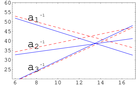
FIG. 2.: $\alpha^{-1}$ as a function of $\log_{10}(M_{G}/M_{Z})$. Unification of couplings for $\Lambda=k$ (solid lines). The standard model is shown for comparison (dashed lines).

VI Conclusions

Unlike in flat extra dimensions, in warped extra dimensions, parameters run logarithmically. This is because one only sees a few KK modes; one does not get the sum of all KK contributions that adds up to power law running [7]. In theories with a cutoff that is high compared to the curvature scale, this running is faster than the standard model; if the cutoff is low, unification is very similar to a four-dimensional model. In this paper, we have presented a procedure for running couplings in AdS₅, and relating high energy parameters to their value at the infrared scale (e.g. $\approx$ TeV). This involved a regularization scheme motivated by AdS/CFT duality and the Wilsonian effective action.

The original Randall-Sundrum scenario was presented as a solution to the hierarchy problem. With bulk gauge bosons, it is now clear that it can also be consistent with coupling constant unification. The key is that even though gauge bosons are in the bulk, running is logarithmic, as in four dimensions. Further details and results are presented in [2].

One might argue that the supersymmetry looks better from the point of view of unification. However, additional threshold corrections are required even in that case for unification, so the net result is also model-dependent, especially when one accounts for the absence of a definite model due to the doublet-triplet splitting problem. It seems fair to say that both scenarios are possibilities at this point and that it is premature to deduce knowledge of physics up to very high energy scales based on unification.

It is clear that there are many possibilities in terms of models and parameters, and the detailed predictions for the high energy couplings from the low energy ones will vary. One can for example consider the supersymmetric version of this theory or alternative GUT groups. Furthermore, we only include the logarithmically enhanced contribution. There are further threshold corrections arising from power law running between $k$ and $\Lambda$, as well as higher order terms in the expansion of $I(\Lambda,q)$. These are of course in addition to the standard subleading corrections. We therefore view this work (and that of [2]) as a first step towards a more detailed and more general analysis.

VII Acknowledgements

We thank Neal Weiner for conversations about GUTs that inspired much of this work. We also wish to thank Nima Arkani-Hamed, Andreas Karch, Emmanuel Katz, Witek Skiba, Yasunori Nomura, Massimo Porrati, and Frank Wilczek for valuable discussions. We also thank Frank for motivation.

REFERENCES

- [1]
- [2] L. Randall and M. D. Schwartz hep-ph/0108114.
- [3] L. Randall and R. Sundrum, Phys. Rev. Lett. 83, 3370 (1999) [hep-ph/9905221].
- [4] I. Antoniadis, N. Arkani-Hamed, S. Dimopoulos and G. Dvali, Phys. Lett. B 436, 257 (1998) [hep-ph/9804398].
- [5] N. Arkani-Hamed, S. Dimopoulos and G. Dvali, Phys. Rev. D 59, 086004 (1999) [hep-ph/9807344].
- [6] N. Arkani-Hamed and S. Dimopoulos, hep-ph/9811353.
- [7] K. R. Dienes, E. Dudas and T. Gherghetta, Nucl. Phys. B 537, 47 (1999) [hep-ph/9806292].
- [8] Y. Nomura, D. Smith and N. Weiner, hep-ph/0104041.
- [9] H. Georgi and S. L. Glashow, Phys. Rev. Lett. 32, 438 (1974).
- [10] A. Pomarol, Phys. Rev. Lett. 85, 4004 (2000) [hep-ph/0005293].
- [11] S. Chang, J. Hisano, H. Nakano, N. Okada and M. Yamaguchi, Phys. Rev. D 62, 084025 (2000) [hep-ph/9912498].
- [12] S. J. Huber and Q. Shafi, Phys. Rev. D 63, 045010 (2001) [hep-ph/0005286].
- [13] T. Gherghetta and A. Pomarol, Nucl. Phys. B 586, 141 (2000) [hep-ph/0003129].
- [14] A. Pomarol, Phys. Lett. B 486, 153 (2000) [hep-ph/9911294].
- [15] H. Davoudiasl, J. L. Hewett and T. G. Rizzo, Phys. Lett. B 473, 43 (2000) [hep-ph/9911262].
- [16] J. Maldacena, Adv. Theor. Math. Phys. 2, 231 (1998) [Int. J. Theor. Phys. 38, 1113 (1998)] [hep-th/9711200].
- [17] E. Witten, Adv. Theor. Math. Phys. 2, 253 (1998) [hep-th/9802150].
- [18] S. S. Gubser, I. R. Klebanov and A. M. Polyakov, Phys. Lett. B 428, 105 (1998) [hep-th/9802109].
- [19] N. Arkani-Hamed, M. Porrati and L. Randall, hep-th/0012148.
- [20] R. Rattazzi and A. Zaffaroni, JHEP 0104, 021 (2001) [hep-th/0012248].
- [21] S. B. Giddings, E. Katz and L. Randall, JHEP 0003, 023 (2000) [hep-th/0002091].
- [22] S. B. Giddings and E. Katz, hep-th/0009176.
- [23] H. Verlinde, Nucl. Phys. B 580, 264 (2000) [hep-th/9906182].
- [24] V. Balasubramanian and P. Kraus, Phys. Rev. Lett. 83, 3605 (1999) [hep-th/9903190].
- [25] H. Cheng, Phys. Rev. D 60, 075015 (1999) [hep-ph/9904252].
- [26] Y. Kawamura, hep-ph/0012125.
- [27] L. Hall and Y. Nomura, hep-ph/0103125.
- [28] P. Langacker, hep-ph/0102085.
- [29] N. Arkani-Hamed, A. Cohen and H. Georgi, hep-th/0108089.
- [30] N. Arkani-Hamed, S. Dimopoulos and J. March-Russell, hep-th/9908146.