Quantum field theory and unification in AdS5
Abstract:
We consider gauge bosons in the bulk of AdS5 in a two-brane theory that addresses the hierarchy problem. We demonstrate that one can do a perturbative calculation above the IR scale associated with the second brane. We show such a theory can be consistent with gauge coupling unification at a high scale. We discuss subtleties in this calculation and show how to regulate consistently in a bounded AdS5 background. Our regularization is guided by the holographic dual of the calculation.
1 Introduction
In AdS5, the coupling for bulk gauge bosons runs logarithmically, not as a power law. For this reason, one can preserve perturbative unification of couplings. Depending on the cutoff, this can occur at a high scale. We show that although it is difficult to do this calculation in a four-dimensional field theory, one can do it in the full five-dimensional context. In this paper, we consider the running of bulk gauge bosons with energy. We discuss several subtleties in the quantity to be calculated, and in the regularization scheme. Our scheme is based on consistency with the holographic correspondence. We will find that generically, as in the standard model, the couplings almost unify, if the is normalized consistently with a GUT group as in [1], as might be the case under various assumptions for the fundamental physics. For specific choices of cutoff and number of scalar multiplets, there is good agreement with the measured couplings and the assumption of high scale unification.
This addresses one of the apparent weaknesses of the warped extra-dimensional theory that addresses the hierarchy problem, that it appears that one must abandon unification of couplings. This problem has been addressed in the context of large extra dimensions in [2] and [3]. However, even if these mechanisms were to work, one would never have high scale unification. In this paper, we show that the warped scenario that naturally generates the hierarchy [4] also naturally accommodates unification, due to the logarithmic running of the couplings. The scale at which unification occurs depends strongly on the cutoff however; fortunately this is connected to a potentially observable quantity, the number of KK modes.
The calculation we do is similar in some respects to that in [5], in which Pomarol considered bulk gauge boson running but with the assumption that the quarks and leptons live on the Planck brane. He made the nice observation that unification can occur in this scenario. Here, we consider theories that address the hierarchy through the warped geometry. We also assme the existence of a Higgs on the TeV brane to generate weak scale symmetry breaking. Another essential difference in our calculation is in the regularization scheme. We will discuss problems with the effective theory calculation and Pauli Villars regularization. In fact, we will argue that a specific regularization scheme is dictated by the holographic correspondence to four-dimensional field theory.
Our analysis also differs from that suggested in [6]. As we will discuss, the particular quantity we are interested in, the running of the coupling of the massless four-dimensional mode, can only be calculated explicitly from the holographic perspective in a theory in which the TeV brane is explicit. The large tree level logarithmic running does not apply to the running of the zero mode coupling.
The organization of this paper is as follows: first, we introduce the theory and review some of the results of the effective 4D picture. We explore some difficulties with the KK picture for the high scale calculation required for running the couplings. In section 4, we derive the position/momentum space propagators in the gauges. We then present some of the Feynman rules and in section 6 we explore the position/momentum space Green’s functions in various limits. We introduce and motivate our regularization scheme in section 7. Through some toy calculations we show that it is necessary to modify the boundary conditions and renormalize the Green’s functions for energies greater than in addition to introducing a position dependent cutoff. We then set up an illustrative calculaton, the contribution of a scalar field to the vacuum energy. In section 9, we calculate the 1-loop -functions. We use the background field method, where the Ward identities are manifest. Finally, section 10 explores unification in two specific examples. We conclude that coupling constant unification is entirely feasible in a warped 2-brane model.
2 Setup
As in [4], we postulate the presence of a fifth dimension, and an anti-deSitter space metric:
| (1) |
We will generally keep the -dependence explicit and contract 4D fields with . We include two branes: the Planck brane at and the TeV brane at . is related to the size of the extra dimension by , and defines the energy scale on the TeV brane. If we take TeV, we can naturally explain the weak scale in the standard model. The fifth dimension can be integrated out to get an effective four-dimensional theory, valid at energies below . The effective 4D Planck scale is given by
| (2) |
It is generally assumed that and .
Now we put gauge bosons in the bulk. The first question is what is the quantity we wish to calculate. We know we cannot run the coupling on the TeV brane above the strong gravity scale, which is roughly TeV. Furthermore, we are ultimately looking at the zero mode, the only light mode in the theory at energies of order TeV or below. This is important; it means the logarithmic running of the coupling considered in [6, 7] does not apply; it is a result of the sum of all the excited gauge modes, all but one of which are heavy from a low-energy perspective. Therefore, the holographic computation of large threshold corrections does not apply. We are ultimately interested only in the relation of the zero-mode coupling of the four-dimensional theory to the high energy five-dimensional coupling.
3 Effective four-dimensional theory
It is of interest to consider the four-dimensional effective theory. As mentioned above, we will abandon this in favor of the full five-dimensional calculation, but here we discuss the theory and why it is problematic.
The action for a 5D gauge boson is:
| (3) |
Here is a mass term on
the TeV-brane, is a mass term on the Planck brane,
and is the bulk mass. The signs are consistent with our metric
convention (1).
To begin with, we take the bulk boson to be massless, and set . We expand the 5D bosons in terms of an orthonormal set of KK modes [8]–[12]:
| (4) | |||||
| (5) |
The expansion of is chosen to diagonalize the couplings between and (see below). Keep in mind that the mass dimensions are , , , , and . The eigenfunctions satisfy:
| (6) |
and therefore have the form:
| (7) |
We assume that the 5D boson, and all the KK modes, have even parity under the orbifold transformation. Consequently their derivatives must vanish on both boundaries. That is, even parity leads to Neumann boundary conditions. Similarly, odd parity leads to Dirichlet boundary conditions, which we will discuss in more detail later on. This leads to the quantization condition:
| (8) |
For , blows up, and so the masses are basically determined by the zeros of . Therefore, they are spaced in energy by approximately . This spacing is quite general: it is independent of bulk or boundary mass terms, and of the spin of the bulk field; because oscillates with the same period for any , bulk fields will always have excitations of order .
We chose the conditions (4), (5) and (6) to normalize the kinetic terms and diagonalize the couplings in the effective 4D action:
| (9) |
This action is explicitly gauge invariant. Indeed, the 5D gauge invariance
| (10) |
has its own KK decomposition (we expand ):
We can plug this back into the action to see that each mode of the 5D gauge field has an independent gauge freedom.
At this point, it is standard to set . We see immediately that this breaks all but the zero mode of the gauge invariance (there is no since ). All modes of are eaten by the corresponding excited modes of the gauge boson. This is the unitary gauge. The Goldstone boson () is eliminated and the massive gauge boson propagators must take the form:
| (11) |
Although this makes the 4D action look very simple, it is problematic for evaluating loop diagrams. When we do the full 5D calculation later on, we will use the Feynman-’t Hooft gauge, in which is included as a physical particle.
Because it will be useful for interpreting our results, we present the mass of the lightest KK modes for states of various spin and mass. For the general lagrangian (3), with arbitrary mass parameters, the spectrum of a bulk gauge boson is determined by:
| (12) |
where . If or is nonzero, the lowest mass is of order . It cannot be lowered below unless or are of the order . For the WZ bosons to pick up a weak scale mass without fine tuning, it must come from the TeV brane. It is not hard to show that for but , the lowest mass is given by [9]:
| (13) |
If TeV, then we can get the weak scale with .
To get a feel for how the spectrum depends on various parameters, we present in table 1 the exact numerical KK spectrum with .
| massless | massive | massive | massive | massless | massless | massive | massless | Dirichlet | |
| vector | vector | vector | vector | Dirichlet | scalar | scalar | Dirichlet | scalar | |
| vector | scalar | ||||||||
| 0 | 2.869 | 6.873 | 1.297 | 3.832 | 0 | 4.088 | 5.136 | 5.434 | |
| 2.458 | 6.086 | 10.762 | 4.134 | 7.016 | 3.832 | 7.321 | 8.417 | 8.739 | |
| 5.575 | 9.249 | 14.196 | 7.213 | 10.174 | 7.016 | 10.498 | 11.620 | 11.953 |
The lagrangian for a massive scalar is .
Next, we look the couplings between the KK modes in a non-abelian theory.
| (14) |
where the coupling constants are given by overlap integrals.
| (15) |
In flat space, momentum conservation in the fifth dimension implies that KK number is conserved. For example, would have to vanish, but would not. In curved space this is not true: in general. We can say something for the zero mode, however. Since we have included no masses, its profile is constant and equal to:
| (16) |
Because the ’s are orthonormal and is constant:
| (17) |
If we set , then the effective theory with just the zero mode looks identical to a 4D system. Moreover, the zero mode couples with equal strength to all the KK modes.
It’s easy to get a rough idea of how the coupling would run if we took the effective theory at face value. That is, we assume all the KK modes are separate particles, and we use a 4D regularization scheme. At low energy, below , only the zero mode can run around the loops. As the energy is increased to , modes are visible. The result is power law running, similar to what has been observed in [2] . This is not the correct result.
One possible improvement, suggested by Pomarol in [5], is to regulate with a Pauli-Villars field with a 5 dimensional mass. This field will have a KK spectrum roughly matching the KK spectrum of the gauge boson, except that it will have a heavy mode near its 5D mass instead of a massless zero mode. Thus all the propagators for the KK modes will roughly cancel and only the zero mode will contribute to running. It will turn out that this is superficially similar to the result we will end up getting from the 5D calculation. However, Pauli-Villars requires that we take the mass of the regulator to infinity, in order to decouple the negative norm states. But an infinitely massive field no longer has a TeV scale KK masses, so it no longer is effective as a regulator. Moreover, it has no hope of telling us threshold corrections, as unitary is violated in the regime where the regulator works.
The root of the problem is that the effective theory breaks down at about a TeV, and so the KK picture is not trustworthy at the high energy scales necessary to probe unification. One can calculate on the Planck brane, but one still has to deal with bulk gauge bosons. The holographic calculation would be at strong coupling. A rigorous perturbative approach is to explore the 5D theory directly.
4 5D Position/momentum space propagators
To study the 5D theory, we will work in position space for the fifth dimension, but momentum space for the other four.
4.1 Gauges
Before gauge fixing, the quadratic terms in the 5D lagrangian are:
| (18) |
We would like to set and then choose the Lorentz gauge . But these conditions are incompatible. Instead, we will use the following gauge-fixing functional:
| (19) |
This produces:
| (20) | |||||
We can then read off the equation that the propagator must satisfy:
| (21) |
where is the four-momentum, and
| (22) |
We define ’s propagator as , where
| (23) |
We choose this notation for the following reason. If we had included a bulk mass in , (22) would have been
| (24) |
Then we can interpret (23) as saying that has the Green’s function of a vector boson with bulk mass . For simplicity we will continue to write for the gauge boson.
We can also work out the ghost lagrangian by varying the gauge fixing functional.
| (25) |
Which makes the ghost propagator:
| (26) |
Note that the ghosts do not couple to directly, as they would not couple directly to Goldstone bosons in a conventional spontaneously broken gauge theory.
If we take , we get the unitary gauge. The gauge boson propagator looks like:
| (27) |
The first term is the transverse polarization states of all the KK modes. We can think of the second term as subtracting off the longitudinal form of the zero mode, Then the zero mode’s contribution has just the regular tensor structure. In this gauge, the and ghost propagators are zero. It is easy to imagine how this gauge would make loop calculations very problematic.
is the Lorentz gauge. Here the propagator is purely transverse, and and the ghosts have 4-dimensional propagators:
| (28) |
Finally, is the Feynman-’t Hooft gauge. The propagators are:
| (29) |
This is the most intuitive gauge. The supplies the longitudinal polarizations to the excited modes of .
4.2 Solving the Green’s functions
To solve (22), we first find the homogeneous solution. Defining and , this is:
| (30) |
and are Bessel functions. For positive parity under the orbifold , we must impose Neumann boundary conditions at both branes:
| (31) |
Finally, matching the two solutions over the delta function leads to the fully normalized Green’s function:
| (32) |
where
| (33) |
If the gauge boson has negative parity under the orbifold , then it must satisfy Dirichlet boundary conditions at both branes (hence we will call it a Dirichlet boson). Its Green’s function will have the same form as (32) but with:
| (34) |
Fields of other spin can be derived analogously. For example, the Green’s function for a massless scalar is:
| (35) |
with
| (36) |
In general, for scalars (), fermions () or vectors () and with bulk mass , as in , the Green’s functions are:
| (37) | |||||
where and
| (38) |
Similar results for KK decompositions can be found in [10]. Keep in mind that although and the ghosts are scalars, their propagators involve the spin-1 Green’s function. Intuitively, this is expected because they are necessary for gauge invariance.
We will eventually have to perform a Wick rotation, so that a euclidean momentum cutoff can be imposed on all the components of . To this end, we will need the Green’s functions with . These functions are still real. It is easiest to get them by re-solving equations like (22) with . The result is:
| (39) | |||||
where as before and
| (40) |
5 Feynman rules
It is fairly straightforward to derive the Feynman rules in these coordinates. External particles are specified by their 4-momentum and their position in the fifth dimension. The vertices have additional factors of the metric which can be read off the lagrangian. Both loop 4-momenta and internal positions must be integrated over. The Feynman rules for a non-abelian gauge theory are (in the Feynman-’t Hooft gauge):
| (41) | |||||
| (42) | |||||
| (43) |
where is the standard 4-boson vertex tensor and group structure. Then there are the contributions:
| (44) | |||||
| (45) | |||||
| (46) | |||||
| (47) |
The derivatives and in (45) are to be contracted with the gauge boson lines, while and in (46) are the momenta of the lines. There are no 3 or 4 vertices because of the antisymmetry of . The Feynman rules for other bulk fields can be derived analogously, with due regard for the factors of metric at the vertices. For example, a vertex would have a factor of , while a vertex would go like . Ghosts, which are scalars, technically come from terms compensating for the gauge invariance of , so they have vertices.
6 Limits of the Green’s functions
Before we evaluate the quantum effects, we will study the propagator in various limits. To do this, we find it convenient to work with euclidean momentum. Recall that the Green’s function for the massless vector boson is:
| (48) |
One advantage of this form is that the modified Bessel functions, and , have limits which are exponentials, while the ordinary Bessel functions oscillate.
The first regime we consider is :
| (49) |
This is what we expect; at low energy, only the zero mode of the gauge boson is accessible. Its profile is constant so is naturally independent of and . The factor of is absorbed in the conversion from 5D to 4D couplings.
It is also useful to consider the next term in the small expansion of at a point in the bulk. This will tell us the size of the 4-Fermi operator which comes from integrating out the excited KK modes.
| (50) |
On the Planck brane and TeV branes respectively, it is:
| (51) | |||||
| (52) |
The additional suppression on the Planck brane over the TeV brane can be understood from the KK picture. The light modes have greater amplitude near their masses, which are near the TeV brane. While there are the same number of heavier modes, localized near the Planck brane, these are additionally suppressed by the square of their larger masses. This has been made quantitative by Davoudiasl et al. in [12]. They calculated the equivalent of using the KK mode propagators:
| (53) |
and showed how this number is constrained by precision tests of the standard model:
| (54) |
Using our formula, this forces TeV if fermions are on the TeV brane and GeV if fermions are on the Planck brane (for ).
With mass terms, the Green’s function satisfies:
| (55) |
We can work through the same analysis as in the massless case. We find that if or is not zero, or if is very large, then the propagator is constant at low momentum. For a non-zero bulk mass:
| (56) |
This tells us the strength of the 4-Fermi operators generated by integrating out heavy fields. For example, if we have a unified model where the and bosons get a bulk mass of order , then on the Planck and TeV branes ():
| (57) | |||||
| (58) |
We know that constraints from proton decay force this number to be smaller than . In particular, we are safe on the Planck brane if GeV for any non-zero bulk mass . On the TeV brane, however, there is no value of the bulk mass which will sufficiently suppress proton decay; it is suppressed by at most . We clearly need to prevent this contribution. We discuss this later in the unification section.
Increasing , we find that for , but and :
| (59) |
where is the Euler-Mascheroni constant. This is valid on the Planck brane at for . In particular, it confirms results of [6, 5] that there is a tree level running of the coupling with . For on the TeV brane,
| (60) |
That the propagator goes as instead of in this regime is evidence of what we noted in the effective theory: there are effectively massless modes which contribute at energy . It is also evidence that this propagator is not valid for on the TeV brane.
Next, we look at and . Here the propagator looks like:
| (61) |
The dependence has the same explanation as (60). Note that the propagator vanishes unless and are nearly coincident in the fifth dimension. Finally, we can consider very large energy, :
| (62) |
Since we are at energies much higher than the curvature scale, , we get a result very similar to the propagator in flat space with the fifth dimension bounded at and :
| (63) |
7 Regulating 5D loops
From studying the 5D propagator in the previous section, we have learned that it cannot be trusted for . This is to be expected if the physical cutoff is around , since the cutoff on the momentum integral will scale with position in the fifth dimension. So we understand that we need a position-dependent cutoff on four-dimensional momentum. The obvious way to implement this cutoff is to integrate up to momentum at a point in the bulk. But we will now show that the Green’s function must also be renormalized. The correct procedure is to recompute the Green’s function at an energy with boundary conditions from an effective IR brane at , and then perform the integral.
Consider the following diagram, which contributes to the gauge boson self energy:
| (64) |
We will eventually be concerned with the correction to the zero mode propagator, so we set the external momentum . The low energy propagator is given by (49) which is independent of and . Since the tree level potential is proportional to we make the identification as before. Also, we will assume the Ward identities are still satisfied and pull out a factor of . Then the integral reduces to:
| (65) |
The in front corresponds to the tree level propagator we are modifying. That factor of gets absorbed when we cap the ends with a in a full S-matrix calculation.
Later on, we will calculate this integral exactly, but for now, we only which to elucidate the regularization scheme. So for a toy calculation, we will pretend that there is only a zero mode, and so has the form (49) at all energies. First, suppose we have a flat cutoff, at . We know this is wrong, but if we just have the zero mode, it should give precisely the 4D result. Indeed,
| (66) |
which is just what we want. Now, suppose we cut off at , with this Green’s function. Then we have:
| (67) |
where we have taken in the last step. Only half the contribution of the zero mode shows up because at an energy , we are only including of it.
Now suppose the IR brane were at instead of . Then, at any energy, there would always be an entire zero mode present. The Green’s function would not have a sharp cutoff, but would get renormalized with Neumann boundary conditions appropriate to its energy scale. Of course, the physical brane is still at , but the Green’s function sees the cutoff as an effective brane. With this regularization, our integral is:
| (68) |
For further illustration, we can work with the full propagator, instead of just the zero-mode approximation, using our new regularization scheme. It is natural to split the integral into two regions, where the propagator can be well-approximated. We can use (59) for small and (61) for large . The small region gives, cutting off at :
| (69) |
This is the contribution of one gauge boson, although it is not exactly the ground state. The large region gives:
| (70) |
This represents, roughly, the additional contribution from the excited modes. In total, there is a log piece, similar to the 4D log but enhanced by a factor of . and a constant piece proportional to . For relatively low values of , the logarithm will dominate, and theory looks four-dimensional. The constant piece contributes to threshold corrections. Later on, when we calculate the -function exactly in section 10, we will find similar qualitative understanding to this rough analytic approximation.
Our regularization scheme applies just as well to higher-loop diagrams. We can define the Green’s function as normalized with a brane at , and zero for . This automatically implements the cutoff, and we don’t have to worry about how to associate the of a vertex with the momentum of a line.
As a final justification of our regularization scheme, we can look at a renormalization group interpretation through AdS/CFT [13, 14]. It is well known that scale transformations in the CFT correspond to translations in . But a scale transformation in a quantum field theory is implemented by a renormalization group flow. It follows that integrating out the high-momentum degrees of freedom in the 4D theory should correspond to integrating out the small region of the 5D theory. Suppose our 5D lagrangian is defined at some scale . This scale is associated not only with the explicit couplings in the lagrangian, but also the boundary conditions with which we define the propagators. The high energy degrees of freedom are not aware of the region with , which includes the TeV brane. Therefore, we are forced to normalize the propagators with an effective virtual brane at . In this way, we derive the low-energy wilsonian effective action in five dimensions. If we follow this procedure down to energies of order TeV, we can then integrate over the fifth dimension to derive the four-dimensional effective theory.
8 Corrections to the radion potential
As a sample calculation, we compute a two-loop contribution to the vacuum energy that determines the radion potential [15, 16]. Consider the following diagram contributing to the vacuum energy of a scalar:
Here is the 5D coupling. which has dimensions of length. It is related to the 4D coupling by . We have cut off the momenta at . The region of integration with or greater than has no dependence, and hence cannot contribute to stabilizing the extra dimension. At low energies,
| (71) |
Note the enhanced dependence of the scalar over the vector propagator (compare (50)). This expansion, which is quite a good approximation of the full propagator in the region of integration we are considering, gives a vacuum energy (ignoring the numerical constants):
| (72) |
This expression has the same -dependence as zero point energy presented in [17].
9 Gauge boson self-energy
In order to address the question of unification, we will now look at how various bulk fields contribute to the 1-loop -functions. There are 6 diagrams that contribute at 1-loop: 2 gauge boson, 1 ghost, and 3 involving . One of these diagrams is particularly ugly, involving acting on the propagator. After fixing the gauge, evaluating, and summing all these diagrams, we should get a correction to the gauge boson propagator which is transverse. But there is an easier way: the background field method. The idea is to compute the effective action directly, which at 1-loop only involves evaluating functional determinants. Furthermore, we have the freedom to choose the external field to be whatever we like. In particular, we can choose it to be the piece of which is independent of . We will see that the quantum fields for , and ghosts effectively decouple. The Ward identities will be explicitly satisfied, as the diagrams containing each type of particle will separately produce a transverse correction to the propagator.
9.1 Background field lagrangian
First, we separate the gauge field into a constant external piece and a fluctuating quantum piece:
| (73) |
We have also renormalized out the coupling. Note that now has mass dimension as in four-dimensions. If we let be the covariant derivative with respect to only then
| (74) |
We also must take our gauge fixing functional to be -covariant:
| (75) |
The lagrangian is then:
| (76) | |||||
At 1-loop, we only need to look at terms quadratic in the quantum fields . After an integration by parts, the quadratic lagrangian is:
| (77) | |||||
We derive the ghost lagrangian from variations of :
| (78) |
Combining (77) with the ghost lagrangian, using the relation
| (79) |
the final quadratic lagrangian for the pure non-abelian gauge theory in is:
| (80) | |||||
Observe that the cross terms between and vanish, as expected. At this point, we will specialize to the function calculation we are interested in. It involves an external zero mode of , whose profile is constant in the fifth dimension. We simply the external field to be the piece of the original field which is independent of . We also set . as there is no external component. This lets us write instead of . Then in the Feynman gauge, , the lagrangian is:
| (81) | |||||
We see immediately that the fields have the propagators we derived before (29), in the Feynman-’t Hooft gauge. There are no cross terms between and and we can evaluate the functional determinant for each field independently. In particular, is seen as a scalar field transforming in the adjoint representation of the gauge group, with the same Green’s function as a vector with bulk mass .
9.2 Functional determinants
We can now evaluate the functional determinants using standard textbook techniques [18]. There are two diagrams which contribute, one is spin-dependent (from the vertex in (81)) and vanishes for scalars, and the other is spin-independent. (The third diagram from the quartic interaction does not contribute as in dimensional regularization, so we will ignore it for simplicity.) Both diagrams are independently transverse in the external momentum. This is evidence that the Ward identity for the 5D gauge invariance is working.
The spin-dependent diagram gives:
| (82) | |||||
where for vectors and zero for scalars and is Dynkin index for the appropriate representation. Since we are interested in the vacuum polarization in the limit, and the transverse projector is already manifest, we can simply set in the integrals. Now change variables to and and set . Then the second line above becomes
| (83) |
The point of doing this is that the integrand now contains the square of:
| (84) |
The in cancels the prefactor in (83), leaving a dimensionless number multiplying the standard 4D integral. This is not strictly true, as still has a weak dependence on . But quite generally, we can write , so for is a fine approximation. Anyway, the background field method at 1-loop cannot give us reliable information about additional divergences, or threshold corrections. The best we can do is to use the degree to which is not constant as a rough measure of the size of the additional corrections.
The other diagram, which is spin-independent. contributes:
| (85) |
where is the number of spin components. The second line is exactly the same integral expression, , as before. While the tensor structure of the first line is not explicitly transverse in the external momentum, it is in fact transverse after the integral is performed (in dimension regularization as ).
Each particle will have a different value for . We must replace with the appropriate propagator (cf. section 4.2) for each particle and redo the integrals in each case. We shall call the result , corresponding to from section 4.2. Observe that as with the gauges, and the ghosts have kinetic terms corresponding to spin 1, so they will both have . In particular, for ghosts is identical to for .
The reason these diagrams are relevant is that they directly produce terms in the effective action. Indeed, the Fourier transform of the quadratic terms in is:
| (86) |
Since is independent of , we have performed the -integral explicitly. So we see that we have calculated a correction to the dimensionless coupling . Equivalently, we have calculated the running of itself, once we absorb the factor of into the coefficient of the logarithm. The result for the 1-loop -function is:
| (87) |
It may appear that we have calculated the running for only the zero mode of the 5D gauge boson. But gauge invariance implies that there can only be one 5D coupling, at any energy scale. So we have in fact calculated the function of every mode. If we define , then the 4D -function is:
| (88) |
Note that the sign of the contribution is opposite to that of the ghosts (which contribute to the above expression). This is because they have opposite statistics which changes the sign of the exponent of the functional determinant. It is easy to understand this result; the ghosts remove the two unphysical polarizations of , and adds back one of them.
9.3 Numerical results for

The function is shown in figure (1), and is shown in figures 2 and 3. Since we need need to perform a Wick rotation to evaluate the 4D integrals, we used the euclidean propagators in calculating . Of course, the constant piece, , is independent of , and we have confirmed this numerically. It turns out that the integrals converge faster in euclidean space. We can see from figure 1 that is roughly proportional to the number of KK modes running around the loop. Because of our boundary conditions, the effective spacing between the KK modes at an energy is . For the massless 5D vector, at energy there is a massless mode, plus approximately other modes visible. This fits roughly with figure 1. The discrepancy is due to the fact that the spacing is not precisely for the lowest modes, and that the sum of the higher modes is not completely negligible. Notice that the ’s of massive and Dirichlet cases, which have no massless zero mode, are about 1 less than for the massless vector. When is bigger than , and the -function is correspondingly higher, the unification scale will be lower. A theory of accelerated unification was also considered in ref. [19] in a different scenario.


Figures 2 and 3 can be understood similarly. As , the branes approach each other. For the massless case, there is always one complete mode, the zero mode. In this limit the theory looks 4-dimensional. For the massive case, the zero mode exists as well, and so it approximates the massless case. With Dirichlet conditions, the zero mode is eliminated, so the function goes to zero. Note that if we had left the boundary conditions at , this function would have gone to zero as for any of the cases. We list the values of for various cases in table 2.
Recall that in the Feynman gauge, ghosts and get the of vectors and has an effective mass . The numbers in this table can be predicted approximately from the KK masses in table 1. We can see that is approximately the number of modes with mass less than . This gives us a very useful intuition for seeing how changing the field content affects unification, as we will now illustrate.
| massless | massive | massive | massive | massless | massless | massive | massless | Dirichlet | |
| vector | vector | vector | vector | Dirichlet | scalar | scalar | Dirichlet | scalar | |
| vector | scalar | ||||||||
| 1.007 | 0.001 | 0.000 | 0.018 | 0.000 | 1.000 | 0.000 | 0.000 | 0.000 | |
| 1.024 | 0.013 | 0.001 | 0.147 | 0.005 | 1.005 | 0.004 | 0.002 | 0.001 | |
| 1.954 | 0.820 | 0.178 | 1.411 | 0.581 | 1.581 | 0.525 | 0.353 | 0.315 |
10 Coupling constant unification
In order to study coupling constant unification, we need to choose a particular model. Because the main motivation of this work is to solve the hierarchy problem using the warp factor, all weak-scale masses should generated from Higgs scalars confined to the TeV brane. We will consider three possible scenarios. The first is that there is no unified group. Indeed, the generic prediction of fundamental theories is only that there should be one coupling constant at high energy, not that there should be a unified group. We put the 3-2-1 gauge bosons in the bulk, and the Higgs and fermions on the TeV brane. From the CFT point of view, the TeV brane fields are to be viewed as condensates. So we can expect there to be a number of bulk fermions or scalars transforming as electroweak doublets, which condense to form the Higgs. In this case, We have to assume there is at a fundamental level a reason to assume the is normalized in a way consistent with a GUT model. For this, additional physics assumptions are necessary.
A second possibility is that there is a unified group, such as . If the doublet Higgs is part of a larger multiplet, such as a vector , then the triplet will necessarily have TeV scale excitations, leading to proton decay. This is the standard doublet-triplet problem [20]. One 4D solution is to couple the triplet to a missing partner, which gives it a large mass and decouples it from the standard model. However, this solution will not work with a TeV brane triplet, because its mass can be at most TeV. Instead, one can for example implement the pseudoGoldstone boson method, as in [20, 21]. Briefly, the idea is to postulate a weakly gauged global symmetry, such as . This is broken by an adjoint and two fundamentals and . The doublet Higgs arises as a pseudoGoldstone boson, and there is no triplet at all. This sort of condensation also seems likely from the CFT point of view, where all TeV brane fields are composites.
Dimension 6 operators that violate baryon number pose a potential problem. As mentioned before, the and bosons should not couple on the TeV brane. This can be done by having the gauge symmetry not commute with the orbifold transformation [22, 23] so that the have positive parity under , but the have negative parity and have vanishing amplitude on the TeV brane. An additional baryon number symmetry should be imposed on the brane to forbid dangerous operators. Notice that the on the brane might have a kinetic term, and therefore a coupling, not determined by unification. If this is the case, one would hope the brane couplings for , , and are all big so that a mechanism such as the one in [24] would apply.
A third possibility is that we don’t use the TeV brane to generate the weak scale, as in [5]. The hierarchy problem must be solved some other way, such as using supersymmetry.
Now return to the first scenario, with no unified group. The TeV-brane particles will contribute to running only up to . After this, they contribute like the bulk fields which represent their preonic constituents in the CFT. There are many possibilities for what these can be, but for the sake of illustration, we will assume they are either fermions or scalars which have the 3-2-1 quantum numbers of the standard model Higgs. Then the 1-loop -functions lead to the following running:
| (89) | |||||
| (91) |
The terms come from the contribution of which has an effective bulk mass . is roughly equal to the number of KK modes with mass below . It is defined exactly in the previous section. There are additional terms in the above equations proportional to , which we will assume to be small. For (which occurs as ), these are just the standard equations for 4 dimensional running. For bulk scalars, the effect is . If the bulk preons are majorana fermions, which would prevent them from picking up a large bulk mass, then this term should be , where comes from 5D massless fermion loops, and the factor of 2 is because fermions contribute twice as much as complex scalars to the gauge boson self-energy. The same modifications should be made for the term, but these do not affect unification, so we will ignore them.
To show that unification can be improved, we pick a specific model. We choose and put 4 majorana fermions in the bulk. We leave , to facilitate the comparison with the standard model. Then we use the numerical values: , , . We will use the observed values [25] of , , and at the Z-boson mass GeV. The couplings are shown for this case in figure 4. The standard model is shown for comparison.
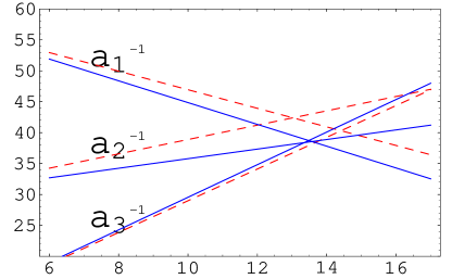
As is increased, and grow at roughly the same rate. The net effect is that the -functions basically scale uniformly with . This will not have much of an effect on whether unification occurs, but it can drastically change the scale, For example, if we take , the scale drops from to . So, if we expect unification near the string scale, we must have . We assumed that was constant. As we mentioned before, the additional effect from the first order term, is suppressed by . So if it is negligible, but if , it can be significant. Even though our regularization scheme cannot tell us the precise effect from the 1-loop calculations, we can easily determine the sign. is the the slope of the curves in figure 2, and is always negative. So for , these corrections will lower the unification scale.
Now consider the second scenario, where the bosons are decoupled from the standard model by changing their parity. Then the coefficient of the log picks up an additional piece, proportional to , as listed in the massless Dirichlet vector column of table 2. Since complete multiplets do not contribute to unification, we can simplify equations (89)–(91) by substituting:
| (92) |
The main effect of this is that it allows us to go to higher values of without lowering the unification scale too much. For example, , but . This makes rather than as it would be without these additional states. We can also put in fields transforming as adjoints or fundamentals under the GUT group with Dirichlet or Neumann components. There are too many possibilities for us to examine them here, but it is fairly straightforward to work out how they affect unification.
Finally consider the third scenario, where matter is on the Planck brane. Here might be broken by a massive adjoint in the standard way, and the triplet might be coupled to some heavy missing partners. Proton decay is suppressed by at least , as we can see from (57). Unification is similar to the second scenario, but we must make the replacement in equations (89)–(91). From table 2, we can see that if the bulk mass is , the relevant value is . This yields even for as big as . However, if the bulk mass of and is too large, for example , then , which leads to . It is clear that there is a lot of room for detailed model building, which we leave for future work.
11 Conclusions
We have shown how to consistently perform Feynman diagram calculations in five-dimensional anti-de Sitter space. Our regularization scheme is inspired by AdS/CFT duality [26, 27, 28]. There we see that scale transformations in the 4D theory are equivalent to z-translations in the 5D theory. Therefore, we can understand how following the renormalization group flow down to the scale corresponds to integrating out the fifth dimension from up to . The correct implementation of this is to renormalize 5D propagators as if the IR brane were at the relevant energy scale for the computation. Not only does this ensure that at a position the UV cutoff is mediated by the warp factor, but also that a complete 4D mode of the bulk field is always present.
The original Randall-Sundrum scenario was presented as a solution to the hierarchy problem. It is now clear that it is also consistent with coupling constant unification. With standard model matter confined to the TeV brane, the maximum unification scale is naively seen to be . From the CFT picture, we know this cannot be true. Now we understand how higher scales are reached in 5D as well. We have briefly described some possible unification scenarios. None of them are perfect, and more detailed model building is called for, but it is clear that unification can be improved from the standard model. The key is that even though gauge bosons are in the bulk, running is effectively four dimensional.
Although we originally intended to tie up a loose end of the AdS/CFT picture, it seems like we have revealed a whole new tangle. There are many directions to go from here, and the work is to a large degree unfinished. There are many threshold corrections that we have not yet included. These include subleading terms in the background field calculation, subleading terms in , and a higher loop calculation. Furthermore, the answer depends on the details of the model; here it is not only a question of the GUT group, but also the bulk fields that yield the TeV brane matter. It is well known that while supersymmetric GUTs appear to unify beautifully at 1-loop, at 2-loops unification does not occur within experimental bounds (without involved model building). It is important to see in more detail how well unification works in this model. Finally, we have been somewhat lax about the relationships among the various scales in the theory, namely and the string scale. These should ultimately be incorporated. Of course, we would also want to motivate in a particular model, and furthermore understand the origin of unification and its scale at a fundamental level.
Acknowledgments.
We would like to thank N. Arkani-Hamed, A. Karch, E. Katz, M. Porrati, and F. Wilczek for useful conversations. We especially thank N. Weiner for helping to initiate this work.References
- [1] H. Georgi and S.L. Glashow, Unity of all elementary particle forces, Phys. Rev. Lett. 32 (1974) 438.
- [2] K.R. Dienes, E. Dudas and T. Gherghetta, Grand unification at intermediate mass scales through extra dimensions, Nucl. Phys. B 537 (1999) 47 [hep-ph/9806292].
- [3] N. Arkani-Hamed, S. Dimopoulos and J. March-Russell, Logarithmic unification from symmetries enhanced in the sub-millimeter infrared, hep-th/9908146.
- [4] L. Randall and R. Sundrum, A large mass hierarchy from a small extra dimension, Phys. Rev. Lett. 83 (1999) 3370 [hep-ph/9905221].
- [5] A. Pomarol, Grand unified theories without the desert, Phys. Rev. Lett. 85 (2000) 4004 [hep-ph/0005293].
- [6] N. Arkani-Hamed, M. Porrati and L. Randall, Holography and phenomenology, J. High Energy Phys. 08 (2001) 017 [hep-th/0012148].
- [7] S. Dimopoulos, S. Kachru, N. Kaloper, A.E. Lawrence and E. Silverstein, Small numbers from tunneling between brane throats, hep-th/0104239.
- [8] S. Chang, J. Hisano, H. Nakano, N. Okada and M. Yamaguchi, Bulk standard model in the Randall-Sundrum background, Phys. Rev. D 62 (2000) 084025 [hep-ph/9912498].
- [9] S.J. Huber and Q. Shafi, Higgs mechanism and bulk gauge boson masses in the Randall-Sundrum model, Phys. Rev. D 63 (2001) 045010 [hep-ph/0005286].
- [10] T. Gherghetta and A. Pomarol, Bulk fields and supersymmetry in a slice of AdS, Nucl. Phys. B 586 (2000) 141 [hep-ph/0003129].
- [11] A. Pomarol, Gauge bosons in a five-dimensional theory with localized gravity, Phys. Lett. B 486 (2000) 153 [hep-ph/9911294].
- [12] H. Davoudiasl, J.L. Hewett and T.G. Rizzo, Bulk gauge fields in the Randall-Sundrum model, Phys. Lett. B 473 (2000) 43 [hep-ph/9911262].
- [13] H. Verlinde, Holography and compactification, Nucl. Phys. B 580 (2000) 264 [hep-th/9906182].
- [14] V. Balasubramanian and P. Kraus, Spacetime and the holographic renormalization group, Phys. Rev. Lett. 83 (1999) 3605 [hep-th/9903190].
- [15] W.D. Goldberger and M.B. Wise, Modulus stabilization with bulk fields, Phys. Rev. Lett. 83 (1999) 4922 [hep-ph/9907447].
- [16] C. Csáki, M.L. Graesser and G.D. Kribs, Radion dynamics and electroweak physics, Phys. Rev. D 63 (2001) 065002 [hep-th/0008151].
- [17] W.D. Goldberger and I.Z. Rothstein, Quantum stabilization of compactified , Phys. Lett. B 491 (2000) 339 [hep-th/0007065].
- [18] We follow the approach and notation of section 16.6 of M. Peskin and D. Schroeder An introduction to quantum field theory Addison-Wesley, 1995.
- [19] N. Arkani-Hamed, A.G. Cohen and H. Georgi, Accelerated unification, hep-th/0108089.
- [20] L. Randall and C. Csáki, The doublet-triplet splitting problem and higgses as pseudogoldstone bosons, hep-ph/9508208.
- [21] H.-C. Cheng, Doublet-triplet splitting and fermion masses with extra dimensions, Phys. Rev. D 60 (1999) 075015 [hep-ph/9904252].
- [22] Y. Kawamura, Triplet-doublet splitting, proton stability and extra dimension, Prog. Theor. Phys. 105 (2001) 999 [hep-ph/0012125].
- [23] L.J. Hall and Y. Nomura, Gauge unification in higher dimensions, Phys. Rev. D 64 (2001) 055003 [hep-ph/0103125].
- [24] N. Weiner, Unification without unification, hep-ph/0106097.
- [25] P. Langacker, Physics implications of precision electroweak experiments, hep-ph/0102085.
- [26] J. Maldacena, The large- limit of superconformal field theories and supergravity, Adv. Theor. Math. Phys. 2 (1998) 231 [hep-th/9711200].
- [27] E. Witten, Anti-de Sitter space and holography, Adv. Theor. Math. Phys. 2 (1998) 253 [hep-th/9802150].
- [28] S.S. Gubser, I.R. Klebanov and A.M. Polyakov, Gauge theory correlators from non-critical string theory, Phys. Lett. B 428 (1998) 105 [hep-th/9802109].
- [29] M.J. Duff and J.T. Liu, Complementarity of the Maldacena and Randall-Sundrum pictures, Phys. Rev. Lett. 85 (2000) 2052 [hep-th/0003237].
- [30] R. Rattazzi and A. Zaffaroni, Comments on the holographic picture of the Randall-Sundrum model, J. High Energy Phys. 04 (2001) 021 [hep-th/0012248].
- [31] S.B. Giddings, E. Katz and L. Randall, Linearized gravity in brane backgrounds, J. High Energy Phys. 03 (2000) 023 [hep-th/0002091].
- [32] S.B. Giddings and E. Katz, Effective theories and black hole production in warped compactifications, hep-th/0009176.
- [33] D.J. Toms, Quantized bulk fields in the Randall-Sundrum compactification model, hep-th/0005189.
- [34] J. Garriga, O. Pujolas and T. Tanaka, Radion effective potential in the brane-world, Nucl. Phys. B 605 (2001) 192 [hep-th/0004109].
- [35] I. Antoniadis, N. Arkani-Hamed, S. Dimopoulos and G.R. Dvali, New dimensions at a millimeter to a fermi and superstrings at a TeV, Phys. Lett. B 436 (1998) 257 [hep-ph/9804398].
- [36] N. Arkani-Hamed, S. Dimopoulos and G.R. Dvali, Phenomenology, astrophysics and cosmology of theories with sub-millimeter dimensions and TeV scale quantum gravity, Phys. Rev. D 59 (1999) 086004 [hep-ph/9807344].
- [37] N. Arkani-Hamed and S. Dimopoulos, New origin for approximate symmetries from distant breaking in extra dimensions, hep-ph/9811353.