BROWN-HET-1276

CU-TP-1025

hep-th/0108006

Probing Black Holes in Non-Perturbative Gauge Theory

Norihiro Iizuka¹, Daniel Kabat¹, Gilad Lifschytz² and David A. Lowe³

¹Department of Physics

Columbia University, New York, NY 10027

iizuka, kabat@phys.columbia.edu

²Department of Mathematics and Physics

University of Haifa at Oranim, Tivon 36006, ISRAEL giladl@research.haifa.ac.il

³Department of Physics

Brown University, Providence, RI 02912

lowe@het.brown.edu

We use a 0-brane to probe a ten-dimensional near-extremal black hole with $N$ units of 0-brane charge. We work directly in the dual strongly-coupled quantum mechanics, using mean-field methods to describe the black hole background non-perturbatively. We obtain the distribution of W boson masses, and find a clear separation between light and heavy degrees of freedom. To localize the probe we introduce a resolving time and integrate out the heavy modes. After a non-trivial change of coordinates, the effective potential for the probe agrees with supergravity expectations. We compute the entropy of the probe, and find that the stretched horizon of the black hole arises dynamically in the quantum mechanics, as thermal restoration of unbroken $U(N+1)$ gauge symmetry. Our analysis of the quantum mechanics predicts a correct relation between the horizon radius and entropy of a black hole.

1 Introduction

For many years it has been an outstanding challenge to develop a microscopic understanding of black hole physics. Many properties of black holes can be easily understood using classical or semiclassical gravity. For example the notion of a horizon arises in classical gravity, while semiclassical considerations show that a horizon has an associated thermodynamic entropy. But ultimately we must understand how these semiclassical properties arise from a microscopic theory of quantum gravity.

The development of non-perturbative definitions of string theory [1] has given a new perspective on these problems. In particular string theory in the background of a ten-dimensional non-extremal black hole with $N$ units of 0-brane charge is known to have a dual description in terms of $U(N)$ gauged supersymmetric quantum mechanics with sixteen supercharges [2]. We would like to understand how the semiclassical physics of black holes emerges from the dual quantum mechanics. Can we recover the classical geometry of the black hole? Can we understand the horizon in terms of microscopic physics? Can we account for the Hawking-Bekenstein entropy?

These questions are not easily answered, because the dual quantum mechanics is strongly coupled whenever semiclassical supergravity is valid [2]. In some cases, one can rely on supersymmetric non-renormalization theorems to calculate at strong coupling [3]. But to make progress in a more general setting, we need non-perturbative methods to study the quantum mechanics.

In [4, 5] we developed a mean-field approximation scheme for the quantum mechanics of $N$ D0-branes. Similar techniques have been applied to matrix integrals in [6]. The approximation can be applied at strong coupling, and gives results for thermodynamic quantities which are in good agreement with semiclassical black hole predictions, at least over a certain range of temperatures. This supports the claim that the dual quantum mechanics can account for the Hawking-Bekenstein entropy. But to address the other questions listed above, we need a probe that is sensitive to the geometry of the black hole.

In the present paper, we introduce an additional D0-brane as a probe of the black hole geometry. It is easy to describe the probe in terms of classical supergravity. In the dual quantum mechanics, the description is in terms of a gauge theory spontaneously broken to $U(N)\times U(1)$. We will make use of our mean-field approximation to describe the quantum mechanics of the $U(N)$ black hole background. There are a number of interesting questions that we can address in this setting. Can one describe a localized probe in the quantum mechanics? Can one recover the expected effective potential for the probe? What physics is responsible for the horizon of the black hole?

An outline of this paper is as follows. In section 2 we review the supergravity description of a D0-brane probe of the black hole background. In section 3 we apply mean-field methods to the dual quantum mechanics problem, and show that we can localize the probe by introducing a resolving time in the quantum mechanics. In section 4 we perform a spectral analysis of 2-point functions in the quantum mechanics, to obtain the microscopic density of single-string excitations. We show that light states are present at the horizon; thus the horizon can be understood as thermal restoration of unbroken $U(N+1)$ gauge symmetry in the quantum mechanics. In section 5 we show that the effective potential for the probe agrees with supergravity expectations. The microcanonical entropy of the probe is computed in section 6. In section 7 we show that our results imply a correct relation between the horizon radius and entropy of a black hole. Section 8 gives some conclusions and directions for future work.

2 Supergravity predictions

We begin with a review of the supergravity description of the probe / black hole system. We will be able to extract a number of useful predictions about the behavior of the dual quantum mechanics.

Our focus will be on the near-horizon region of a ten-dimensional non-extremal black hole in type IIA supergravity. The black hole is taken to have $N$ units of D0-brane charge, so that the dual quantum mechanics is $U(N)$ gauged supersymmetric quantum mechanics with sixteen supercharges [2]. In the near-horizon region the string-frame metric of the black hole is given by

$$ds^{2} = \alpha^{\prime}\left[-h(U)dt^{2}+h^{-1}(U)dU^{2}+{c^{1/2}(g_{YM}^{2}N)^{1/2}\over U^{3/2}}d\Omega_{8}^{2}\right]$$

$$h(U) = \frac{U^{7/2}}{c^{1/2}(g_{YM}^{2}N)^{1/2}}\left(1-\frac{U_{0}^{7}}{U^{7}}\right)$$ (1)

where $c=2^{7}\pi^{9/2}\Gamma(7/2)$ and $g^{2}_{YM}=g_{s}/4\pi^{2}(\alpha^{\prime})^{3/2}$ is the coupling constant of the dual gauge theory. The dilaton profile is given by

$$e^{\phi}={1\over(\alpha^{\prime})^{3/2}}\left({cg^{2}_{YM}N\over U^{7}}\right)^{3/4}$$ (2)

and there is a R-R 1-form potential [8]

$$A_{0}=1+\frac{(\alpha^{\prime})^{2}U^{7}}{cg^{2}_{YM}N}\left(-1+{U_{0}^{7}\over 2U^{7}}\right)+{\cal O}(\alpha^{\prime}{}^{4})\,.$$ (3)

The horizon of the black hole is located at $U=U_{0}$, which corresponds to a Hawking temperature

$$T={7\over 2\pi\sqrt{30}}~{}(g^{2}_{YM}N)^{-1/2}\left(U_{0}\over 2\pi\right)^{5/2}=0.2034~{}(g^{2}_{YM}N)^{-1/2}\left(U_{0}\over 2\pi\right)^{5/2}\,.$$ (4)

This is the temperature measured with respect to the Schwarzschild time coordinate $t$. Since $t$ is identified with the time coordinate of the dual gauge theory, the dual quantum mechanics is to be studied at the same finite temperature. The black hole has a free energy [9]

$$\beta F=-\left({2^{21}3^{2}5^{7}\pi^{14}\over 7^{19}}\right)^{1/5}\!\!N^{2}\left({T\over(g_{YM}^{2}N)^{1/3}}\right)^{9/5}=-4.115~{}N^{2}\left({T\over(g_{YM}^{2}N)^{1/3}}\right)^{1.8}\,.$$ (5)

Duality predicts that the quantum mechanics should have the same free energy. The supergravity description is expected to be valid when the curvature and the dilaton are small near the black hole horizon. This regime corresponds to the ’t Hooft large-$N$ limit of the quantum mechanics, together with the requirement that the effective ’t Hooft coupling in the quantum mechanics

$$g_{\rm eff}^{2}=g^{2}_{YM}N/T^{3}$$ (6)

lies in the range

$$1\ll g_{\rm eff}^{2}\ll N^{10/7}\,.$$ (7)

Note that the quantum mechanics is strongly coupled whenever semiclassical supergravity is valid [2].

A 0-brane probe of this supergravity background is described by the action

$$S=-T_{0}\int dt\,e^{-\phi}\sqrt{-\det G}-T_{0}\int dtA_{0}$$ (8)

where the tension of a 0-brane is $T_{0}=1/g_{s}\sqrt{\alpha^{\prime}}$. Evaluating this on the black hole background (1) – (3) gives the effective action for the probe in the decoupling limit [7, 8]

$$S = -{1\over 4\pi^{2}g^{2}_{YM}}\int dt\,\mathopen{{\hbox{$\left missing\vbox to25.0pt{}\right.$}}}[{U^{7}\over cg^{2}_{YM}N}\left(-1+{U_{0}^{7}\over 2U^{7}}\right)$$

$$+\left({U^{7}\over cg^{2}_{YM}N}\right)^{3/4}\sqrt{h(U)-{1\over h(U)}\dot{U}^{2}-{c^{1/2}(g^{2}_{YM}N)^{1/2}\over U^{3/2}}\dot{\Omega}^{2}}\mathclose{{\hbox{$\left missing\vbox to25.0pt{}\right.$}}}]$$

(we dropped a constant term, the rest energy of the probe at infinity). From the action we can read off the effective potential for a static probe,

$$V_{\rm eff}=-\frac{N}{15(g_{YM}^{2}N)^{2}}\left({U\over 2\pi}\right)^{7}\left(\sqrt{1-{U_{0}^{7}\over U^{7}}}-1\right)^{2}\,.$$ (10)

Note that the effective potential (10) is singular at the horizon of the black hole. A singularity in a low-energy effective action suggests that massless degrees of freedom have been improperly integrated out. To see that this is indeed the case, consider ‘W-bosons’: open strings which can stretch between the probe 0-brane and the black hole. The energy of these strings can be computed by evaluating the Nambu-Goto action

$$S_{NG}=-{1\over 2\pi\alpha^{\prime}}\int d^{2}\sigma\sqrt{-\det G}$$

on a string worldsheet which starts at the horizon and ends on the probe. A straightforward calculation gives an energy, measured with respect to the Schwarzschild time coordinate $t$, equal to

$$m_{W}={1\over 2\pi}\left(U-U_{0}\right)\,.$$ (11)

This is identical to the calculations of [10], performed in the context of studying Wilson lines at finite temperature.

The energy of these strings indeed goes to zero as the probe approaches the horizon. In [11] it was argued that these massless degrees of freedom are responsible for the singularity of the supergravity effective potential (10). We conclude that the supergravity description of the probe breaks down when the probe gets too close to the horizon, at least according to a Schwarzschild observer. In the full string theory (or dual quantum mechanics), which takes these light degrees of freedom into account, the W-bosons will become thermally excited as the probe approaches the horizon.

To estimate the radius of the ‘stretched horizon’ at which this thermalization starts to occur, we compare the energy of a W-boson (11) to the temperature of the black hole (4) (the comparison is meaningful, since both energies are measured with respect to the same Schwarzschild time coordinate $t$). Setting $m_{W}=T$ gives the radius of the stretched horizon

$$U_{\rm stretched}=U_{0}\left(1+{7\over\sqrt{30}(2\pi)^{5/2}}\biggl{(}{U_{0}\over(g^{2}_{YM}N)^{1/3}}\biggr{)}^{3/2}\right)\,.$$ (12)

At this radius stringy degrees of freedom start to become thermally excited, so the supergravity description of the probe breaks down, and the classical black hole geometry (1) is no longer reliable.

For an accurate description of physics inside the stretched horizon, we must turn to the dual quantum mechanics (or full string theory). There we see that light W-bosons are rapidly created, so the probe quickly thermalizes with the black hole. Once the probe 0-brane has come to thermal equilibrium, it can no longer be distinguished from the other 0-branes that make up the black hole.

This makes it easy to compute the energy and entropy of the probe once it has been absorbed by the black hole and come to equilibrium. The effect of the probe is simply to shift $N\rightarrow N+1$ in the semiclassical free energy of the black hole (5). We shift $N$ holding both $g_{YM}$ and the temperature fixed. Thus the free energy of a probe in equilibrium is given by

$$\beta F_{\rm probe}=-5.76N\left(T\over(g^{2}_{YM}N)^{1/3}\right)^{9/5}\,.$$ (13)

This agrees precisely with the free energy one obtains by evaluating the DBI effective potential (10) at the horizon of the black hole, $\beta F_{\rm probe}=\beta V_{\rm eff}|_{U=U_{0}}$. This rather surprising coincidence was noted and explained in [12].

To better understand the absorption process, note that the energy and entropy of a probe in equilibrium can be obtained from the corresponding black hole quantities by shifting $N\rightarrow N+1$. That is, they are given by

$$E_{\rm probe} = \left({2^{21}3^{12}\pi^{14}\over 5^{3}7^{14}}\right)^{1/5}\!\!N(g_{YM}^{2}N)^{1/3}\left({T\over(g_{YM}^{2}N)^{1/3}}\right)^{14/5}$$

$$S_{\rm probe} = \left({2^{26}3^{2}\pi^{14}\over 5^{3}7^{9}}\right)^{1/5}\!\!N\left({T\over(g_{YM}^{2}N)^{1/3}}\right)^{9/5}\!\!\!.$$ (14)

Note that the probe acquires positive energy as it comes to equilibrium with the black hole. This is in sharp contrast to the negative attractive potential (10) which is present outside the stretched horizon. Moreover the probe acquires entropy once it is inside the stretched horizon, associated with the excited W-boson degrees of freedom. By contrast, outside the stretched horizon the probe entropy is very small (according to classical supergravity, it is exactly zero). Thus absorption of the probe by the black hole is driven by the increase in entropy, which more than makes up for the cost in energy.

3 Gauge theory calculations

We now turn to the dual gauge theory description of the probe / black hole system, and apply mean-field methods [5] to study the quantum mechanics at strong coupling.

Our starting point is $U(N+1)$ gauged supersymmetric quantum mechanics with sixteen supercharges [13]. As in our previous work, we will describe the quantum mechanics using the language of ${\cal N}=2$ superspace. This formalism makes ${\cal N}=2$ supersymmetry manifest (out of the underlying ${\cal N}=16$). It also makes manifest a $G_{2}\times SO(2)$ subgroup of the underlying $SO(9)$ rotational invariance.

In terms of ${\cal N}=2$ superfields, the action for 0-brane quantum mechanics reads

$$S={1\over g^{2}_{YM}}\int dtd^{2}\theta\,{\rm Tr}\biggl{(}-{1\over 4}\nabla^{\alpha}{\cal F}_{i}\nabla_{\alpha}{\cal F}_{i}-\frac{1}{2}\nabla^{\alpha}\Phi_{A}\nabla_{\alpha}\Phi_{A}-\frac{i}{3}f_{ABC}\Phi_{A}[\Phi_{B},\Phi_{C}]\biggr{)}\,.$$ (15)

Here $\nabla_{\alpha}$ is a $U(N+1)$ gauge superconnection, and ${\cal F}_{i}$ is the corresponding field strength. The fields

$$\Phi_{A}=\phi_{A}+i\psi_{A\alpha}\theta_{\alpha}+f_{A}\theta^{2}$$

are a collection of seven adjoint scalar multiplets, with $A,\,B=1,\ldots,7$ an index in the ${\bf 7}$ of $G_{2}$, and $f_{ABC}$ is a suitably normalized totally antisymmetric $G_{2}$-invariant tensor. For more details on our notation see appendix A.

3.1 Introducing a localized probe

We wish to use a single 0-brane to probe a black hole with $N$ units of 0-brane charge. To do this we separate the probe from the black hole, by giving an expectation value to one of the scalar fields, say

$$\langle\Phi_{7}\rangle=\left(\begin{array}[]{cc}0&0\\ 0&R\end{array}\right)\,.$$ (16)

Classically this breaks the gauge symmetry from $U(N+1)$ down to $U(N)\times U(1)$, and gives the off-diagonal fields a mass $m_{W}=R$.

Before continuing, there is an important question we must address: is the expectation value (16) meaningful at strong coupling? The issue is that at strong coupling the eigenvalues of $\phi_{A}$ have large quantum fluctuations. These fluctuations can be measured by computing the connected equal-time correlation function ${1\over N}\langle{\rm Tr}(\phi_{A})^{2}\rangle_{C}$. For example in our approximation the eigenvalues obey a Wigner semicircle distribution, with maximum eigenvalue

$$\lambda_{\rm max}=2\sqrt{\langle{\rm Tr}(\phi_{A})^{2}\rangle_{C}/N}\,.$$ (17)

On general grounds one can argue that [14, 15]

$${1\over N}\langle\,{\rm Tr}(\phi_{A})^{2}\,\rangle_{C}\,\sim\,\left(g^{2}_{YM}N\right)^{2/3}\,,$$ (18)

and this behavior is indeed seen in our mean-field approximation [5]. Thus the eigenvalues of $\phi_{A}$ fluctuate over the entire region, of size $\sim(g^{2}_{YM}N)^{1/3}$ [2], in which supergravity is valid. We want to place the probe well inside the supergravity region, at some value of $R\ll(g^{2}_{YM}N)^{1/3}$. But can we really claim to have a well-localized probe, given the large fluctuations (18)?

The answer is that the probe can be well-localized, as long as it is outside the stretched horizon. To see this, note that supergravity only emerges as a low energy approximation to the quantum mechanics. To discuss the position of the probe we must introduce a resolving time, and integrate out the high-frequency degrees of freedom in the quantum mechanics. These high-frequency modes are responsible for the large fluctuations (18), and by integrating them out, we can construct a sharply-defined position operator for the probe.

Following [15], a suitable position operator can be obtained by smearing the Heisenberg picture fields over a Lorentzian time interval $\epsilon$.

$$\bar{\phi}_{A}=\int_{-\infty}^{\infty}{dt\over\epsilon\sqrt{\pi}}e^{-t^{2}/\epsilon^{2}}\phi_{A}(t)$$ (19)

The effect of the resolving time $\epsilon$ is to integrate out modes with frequency larger than $1/\epsilon$. We can only integrate out modes which are not thermally excited, so an appropriate choice of resolving time is $\epsilon\sim\beta$. Then the operators $\bar{\phi}_{A}$ provide sharply-defined position operators for the probe, at least as long as the probe is outside the stretched horizon. As we shall see, as the probe enters the stretched horizon, W-bosons with a mass of order $1/\beta$ start to become thermally excited. These light W-bosons contribute to the fluctuations in $\bar{\phi}_{A}$, so once the probe enters the stretched horizon it cannot be localized to less than the size of the stretched horizon.

Although the probe can be well-localized outside the stretched horizon, one subtle question remains: what is the precise relationship between the Higgs vev $R$ appearing in (16) and the supergravity radial coordinate $U$ appearing in (1)? At zero temperature one can rely on supersymmetry to make a precise identification. The mass of a BPS stretched string in the gauge theory is given exactly by the tree-level formula $m_{W}=R$, while in supergravity the classical formula $m_{W}=U/2\pi$ (11) is not corrected. Therefore one can identify $R=U/2\pi$ at zero temperature. However, this identification is not appropriate at finite temperature. We will work out the correct identification in section 5.

3.2 Mean-field approximation

Having understood the description of a localized probe at strong coupling, we proceed to apply mean-field methods [4, 5] to the quantum mechanics.

The 0-brane action (15) has a manifest $G_{2}$ global symmetry, but the expectation value (16) breaks this to $SU(3)$, so we begin by rewriting the action in form with manifest $SU(3)$ invariance. Under $SU(3)\subset G_{2}$ the ${\bf 7}$ decomposes into ${\bf 3}\oplus\bar{\bf 3}\oplus{\bf 1}$. Thus in place of the seven real scalar multiplets $\Phi_{A}$ we have a set of three complex scalar multiplets $\Phi_{a}$ transforming in the ${\bf 3}$, their adjoints $\Phi_{\bar{a}}^{\dagger}$ in the $\bar{\bf 3}$, and a single real scalar multiplet $\Phi_{7}$. The 0-brane action reads

$$S = {1\over g^{2}_{YM}}\int dtd^{2}\theta\,{\rm Tr}\biggl{\{}-D^{\alpha}\Phi_{\bar{a}}^{\dagger}D_{\alpha}\Phi_{a}-{1\over 2}D^{\alpha}\Phi_{7}D_{\alpha}\Phi_{7}$$

$$\qquad+{1\over 3\sqrt{2}}\epsilon_{abc}\Phi_{a}[\Phi_{b},\Phi_{c}]-{1\over 3\sqrt{2}}\epsilon_{{\bar{a}}{\bar{b}}{\bar{c}}}\Phi_{\bar{a}}^{\dagger}[\Phi_{\bar{b}}^{\dagger},\Phi_{\bar{c}}^{\dagger}]+\Phi_{7}[\Phi_{a},\Phi_{\bar{a}}^{\dagger}]$$

$$\qquad+\,\,\,\hbox{\rm terms involving the gauge connection}\biggr{\}}~{}.$$

We expand about the background (16), setting

$$\Phi_{a} = \left(\begin{array}[]{cc}\hat{\Phi}_{a}&\delta\Phi_{a}\\ \delta\tilde{\Phi}_{a}^{\dagger}&0\end{array}\right)$$ (23)

$$\Phi_{\bar{a}}^{\dagger} = \left(\begin{array}[]{cc}\hat{\Phi}_{\bar{a}}^{\dagger}&\delta\tilde{\Phi}_{\bar{a}}\\ \delta\Phi_{\bar{a}}^{\dagger}&0\end{array}\right)$$ (26)

$$\Phi_{7} = \left(\begin{array}[]{cc}\hat{\Phi}_{7}&\delta\Phi_{7}\\ \delta\Phi_{7}^{\dagger}&R\end{array}\right)$$ (29)

with a similar expansion for the gauge connection. The hatted fields are $N\times N$ matrices describing the black hole background, while the off-diagonal fields describe W-bosons in the fundamental of $U(N)$, and $R$ is the Higgs vev which parameterizes the position of the probe.

Expanding the action in powers of the off-diagonal fields, we have (with $\hat{\Phi}$ referring to all of the scalar multiplets as well as the gauge connection)

$$S=S_{\rm background}(\hat{\Phi})+S_{\rm quadratic}(\hat{\Phi},\delta\Phi)+\ldots\,.$$ (30)

The zeroth order terms describe the black hole background. All first order terms automatically vanish, given the matrix structure (26) and the fact that the action (3.2) involves a single overall trace. We can stop with the quadratic terms in (30), since the off-diagonal fields transform in the fundamental of $U(N)$, which means the higher-order terms make contributions that are suppressed by $1/N$ in the large-$N$ limit.

To get a tractable description of the black hole background, we use our mean-field approximation scheme [5]. In this approximation one constructs a trial action $S_{0}(\hat{\Phi})$, which can be thought of as a variational approximation to the full action $S_{\rm background}(\hat{\Phi})$. We took $S_{0}$ to essentially be the most general quadratic action that one can write in terms of the fundamental background fields. The trial action is therefore characterized by a set of 2-point functions, which were obtained by solving a set of truncated Schwinger-Dyson equations.

To make a mean-field approximation for the background, we replace $S_{\rm background}\rightarrow S_{0}$ in (30). This gives us an effective description of the probe, in terms of the action

$$S=S_{0}(\hat{\Phi})+S_{\rm quadratic}(\hat{\Phi},\delta\Phi)\,.$$ (31)

In principle this action can be solved by standard large-$N$ techniques, since $S_{0}$ is a known quadratic action and the fields $\delta\Phi$ are in the fundamental of $U(N)$. However, for simplicity, we wish to make a further approximation: we will only keep fields which transform in the ${\bf 3}$ or $\bar{\bf 3}$ of $SU(3)$. We will say more about the validity of this truncation in section 5. Given these approximations, the action of interest is explicitly given by

$$S = S_{0}(\hat{\Phi}_{a},\hat{\Phi}^{\dagger}_{\bar{a}})+{1\over g^{2}_{YM}}\int dtd^{2}\theta\,\biggl{\{}-D^{\alpha}\delta\Phi_{\bar{a}}^{\dagger}D_{\alpha}\delta\Phi_{a}-R\delta\Phi_{\bar{a}}^{\dagger}\delta\Phi_{a}$$

$$\quad-D^{\alpha}\delta\tilde{\Phi}_{a}^{\dagger}D_{\alpha}\delta\tilde{\Phi}_{\bar{a}}+R\delta\tilde{\Phi}_{a}^{\dagger}\delta\tilde{\Phi}_{\bar{a}}+\sqrt{2}\epsilon_{abc}\delta\tilde{\Phi}_{a}^{\dagger}\hat{\Phi}_{b}\delta\Phi_{c}-\sqrt{2}\epsilon_{{\bar{a}}{\bar{b}}{\bar{c}}}\delta\Phi_{\bar{a}}^{\dagger}\hat{\Phi}_{\bar{b}}^{\dagger}\delta\tilde{\Phi}_{\bar{c}}\biggr{\}}\,.$$

We are interested in studying this theory at finite temperature. To do this we use an imaginary-time formalism. We adopt the component expansions discussed in appendix A

$$\delta\Phi_{a} = \delta\phi_{a}+i\delta\psi_{\alpha a}\theta_{\alpha}+\delta f_{a}\theta^{2}$$

$$\delta\Phi_{\bar{a}}^{\dagger} = \delta\phi_{\bar{a}}^{\dagger}+i\delta\psi_{\alpha{\bar{a}}}^{\dagger}\theta_{\alpha}+\delta f_{\bar{a}}^{\dagger}\theta^{2}$$

(same for tilded fields). We continue to Euclidean space by setting

$$S_{E}=-iS_{M}\qquad\tau=it_{M}\qquad f_{E}=-if_{M}\,.$$

Note that the auxiliary fields must be Wick rotated to obtain a Euclidean action that is bounded below. (The rotation is somewhat subtle; we need both $\delta f_{aE}=-i\delta f_{aM}$ and $\delta f_{{\bar{a}}E}^{\dagger}=-i\delta f_{{\bar{a}}M}^{\dagger}$). We then compactify Euclidean time on a circle of circumference $\beta$, and expand the fields in Matsubara modes. For example we write

$$\delta\phi_{a}(\tau) = {1\over\sqrt{\beta}}\sum_{l\in{\mathbb{Z}}}\delta\phi_{al}e^{i2\pi l\tau/\beta}$$

$$\delta\psi_{\alpha a}(\tau) = {1\over\sqrt{\beta}}\sum_{r\in{\mathbb{Z}}+1/2}\delta\psi_{\alpha ar}e^{i2\pi r\tau/\beta}\,.$$

The model (3.2) can be solved by standard large-$N$ methods. The leading contribution to the free energy is ${\cal O}(N^{2})$, and comes from the black hole background. The leading contribution to the free energy of the probe is ${\cal O}(N)$, and comes from a single loop of W-bosons. Since the action (3.2) only has 3-point couplings involving two W-bosons and one background field, the W propagator is given exactly by summing rainbow diagrams, just as in the ’t Hooft model of two-dimensional chromodynamics [16]. The mean-field methods used in [4, 5] therefore provide an exact description of the probe, and we shall state the solution to the model using the language of mean-field theory.

At leading order in $1/N$ the properties of the probe are completely characterized by the W propagators. We denote these propagators

$$\langle\delta\phi^{\dagger}_{{\bar{a}}lI}\delta\phi_{bmJ}\rangle_{0} = \Delta_{l}^{2}\delta_{{\bar{a}}b}\delta_{lm}\delta_{IJ}$$

$$\langle\delta f^{\dagger}_{{\bar{a}}lI}\delta\phi_{bmJ}\rangle_{0} = \langle\delta\phi^{\dagger}_{{\bar{a}}lI}\delta f_{bmJ}\rangle_{0}=i\gamma_{l}\delta_{{\bar{a}}b}\delta_{lm}\delta_{IJ}$$ (33)

$$\langle\delta f^{\dagger}_{{\bar{a}}lI}\delta f_{bmJ}\rangle_{0} = \epsilon_{l}^{2}\delta_{{\bar{a}}b}\delta_{lm}\delta_{IJ}$$

$$\langle\delta\psi^{\dagger}_{\alpha{\bar{a}}rI}\delta\psi_{\beta bsJ}\rangle_{0} = ig_{r}\delta_{\alpha\beta}\delta_{{\bar{a}}b}\delta_{rs}\delta_{IJ}+ih_{r}\epsilon_{\alpha\beta}\delta_{{\bar{a}}b}\delta_{rs}\delta_{IJ}$$

(same for tilded fields and propagators) where $I,J$ are indices in the fundamental of $U(N)$. These propagators are to be determined by solving a set of one-loop gap equations, which we give below. The background action $S_{0}(\hat{\Phi})$ is also characterized by a set of 2-point functions, which we denote

$$\langle\hat{\phi}^{\dagger}_{{\bar{a}}lIJ}\hat{\phi}_{bmKL}\rangle_{0} = \hat{\Delta}_{l}^{2}\delta_{{\bar{a}}b}\delta_{lm}\delta_{IL}\delta_{JK}$$

$$\langle\hat{f}^{\dagger}_{{\bar{a}}lIJ}\hat{f}_{bmKL}\rangle_{0} = \hat{\epsilon}_{l}^{2}\delta_{{\bar{a}}b}\delta_{lm}\delta_{IL}\delta_{JK}$$

$$\langle\hat{\psi}^{\dagger}_{\alpha{\bar{a}}rIJ}\hat{\psi}_{\beta bsKL}\rangle_{0} = i\hat{g}_{r}\delta_{\alpha\beta}\delta_{{\bar{a}}b}\delta_{rs}\delta_{IL}\delta_{JK}\,.$$

The action (3.2) has a ${\mathbb{Z}}_{2}$ symmetry which exchanges $\delta\Phi$ and $\delta\tilde{\Phi}$, and takes $R\rightarrow-R$, $\hat{\Phi}\rightarrow-\hat{\Phi}$. This symmetry implies that

$$\Delta_{l}^{2}=\tilde{\Delta}_{l}^{2}\qquad\gamma_{l}=-\tilde{\gamma}_{l}\qquad\epsilon_{l}^{2}=\tilde{\epsilon}_{l}^{2}\qquad g_{r}=\tilde{g}_{r}\qquad h_{r}=-\tilde{h}_{r}\,.$$ (34)

From now on we will use this relation to eliminate the tilded propagators.

The propagators appearing in (33) are to be determined by solving a set of one-loop gap equations. The gap equations can be obtained by demanding that the two-loop 2PI effective action discussed in [4, 5] is stationary with respect to infinitesimal variations of the propagators. The free energy of the probe can then be obtained by evaluating the effective action at the critical point. In the present case, after a rescaling discussed below, the effective action $\beta F$ is given by

$$\beta F=-6\sum_{l}\log\left(\Delta_{l}^{2}\epsilon_{l}^{2}+(\gamma_{l})^{2}\right)+6\sum_{r}\log\left((g_{r})^{2}+(h_{r})^{2}\right)$$ (35)

$$+6\sum_{l}\left(({2\pi l\over\beta})^{2}\Delta_{l}^{2}-2R\gamma_{l}+\epsilon_{l}^{2}-2\right)-12\sum_{r}\left({2\pi r\over\beta}g_{r}-Rh_{r}-1\right)$$

$$+{24\over\beta}\sum_{l+m+n=0}\Delta_{l}^{2}\hat{\Delta}_{m}^{2}\epsilon_{n}^{2}+{12\over\beta}\sum_{l+m+n=0}\Delta_{l}^{2}\hat{\epsilon}_{m}^{2}\Delta_{n}^{2}+{24\over\beta}\sum_{l+m+n=0}\gamma_{l}\hat{\Delta}_{m}^{2}\gamma_{n}$$

$$+{48\over\beta}\sum_{l+r+s=0}g_{r}\hat{g}_{s}\Delta_{l}^{2}+{24\over\beta}\sum_{l+r+s=0}g_{r}\hat{\Delta}_{l}^{2}g_{s}-{24\over\beta}\sum_{l+r+s=0}h_{r}\hat{\Delta}_{l}^{2}h_{s}~{}.$$

The gap equations and effective action are discussed in more detail in appendix B.

Let us briefly note an important feature of our solution. In evaluating the effective action, we only kept planar diagrams. This makes ’t Hooft large-$N$ counting automatic, so the free energy of the probe is guaranteed to be ${\cal O}(N)$. Moreover, the Yang-Mills coupling constant can only appear in the combination $g^{2}_{YM}N$. In (35), and in the rest of this paper, we suppress the overall factor of $N$ in the probe free energy. Also, by rescaling all dimensionful quantities as in appendix B, we effectively adopt units which set $g^{2}_{YM}N=1$.

To solve the gap equations we used the numerical methods described in [5], which we will not review here. The basic idea is to start by solving the gap equations at large $R$, where the theory is weakly coupled, and then use the Newton-Raphson method to solve the gap equations at a sequence of successively smaller radii.

4 Spectral analysis

At leading order in $1/N$ the properties of the probe are completely characterized by the W propagators. In the previous section we described how these are computed numerically, as functions of imaginary time. There are a number of interesting questions that are difficult to address, however, simply given the imaginary time propagators. For example, we would like to determine the masses of the W-bosons, to see if supergravity predictions for the behavior of strings that stretch between the probe and horizon are borne out, and to fix the relation between the supergravity radial coordinate $U$ and the Higgs expectation value $R$. We would also like to determine the entropy of the probe in a fixed black hole background. These things are not easily done in imaginary time.

To address these questions, it is useful to introduce a spectral representation for the W propagators. By inserting complete sets of states one can derive the following analog of the Lehmann-Källen spectral representation for a scalar propagator

$$\langle\phi(\tau)\phi(0)\rangle_{\beta}=\int_{0}^{\infty}d\omega\rho(\omega){\cosh\omega(\tau-\beta/2)\over 2\omega\sinh(\beta\omega/2)}\qquad\quad\hbox{\rm$0\leq\tau\leq\beta$}~{}.$$ (36)

Here the spectral density is given by

$$\rho(\omega)={1\over Z}\sum_{m}e^{-\beta E_{m}}\sum_{n>m}|\langle n|\phi|m\rangle|^{2}\,\,2\omega\left(1-e^{-\beta\omega}\right)\delta(\omega-E_{n}+E_{m})\,.$$

We will apply this spectral decomposition to the fields $\delta\phi_{a}$, writing their momentum-space propagator as

$$\Delta_{l}^{2}=\int_{0}^{\infty}d\omega\rho(\omega){1\over(2\pi l/\beta)^{2}+\omega^{2}}\,.$$ (37)

We can regard $\rho(\omega)d\omega$ as the number of single-string microstates having an energy between $\omega$ and $\omega+d\omega$. By expanding the propagator at large momentum as discussed in appendix B, note that the spectral density should satisfy

$$\int d\omega\rho(\omega)=1\qquad\int d\omega\rho(\omega)\omega^{2}=m_{\Delta}^{2}$$ (38)

where $m_{\Delta}^{2}$ is the asymptotic mass (76).

An interesting problem, motivated by our discussion of supergravity in section 2, is to determine the energies of the lightest and heaviest string states $\omega_{\rm min}$ and $\omega_{\rm max}$. It is easy to put bounds on these quantities, as follows. From (38) we have

$$m_{\Delta}^{2}=\int d\omega\rho(\omega)\omega^{2}\leq\omega_{\rm max}^{2}\,.$$

Also one can use (36) to show that

$$\cosh(\beta\omega_{\rm min}/2)\leq{\langle\phi(0)\phi(0)\rangle_{\beta}\over\langle\phi(\beta/2)\phi(0)\rangle_{\beta}}\,.$$ (39)

Thus we have an upper bound on $\omega_{\rm min}$, and a lower bound on $\omega_{\rm max}$. These bounds are shown in Fig. 1. Note that as the temperature decreases, $\omega_{\rm min}$ develops a rather sharp plateau at small radius. We take this to indicate that the probe has started to come to equilibrium with the black hole, in the range of Higgs vevs corresponding to the plateau.

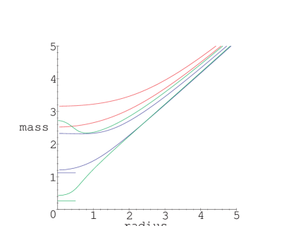
Figure 1: Bounds on $\omega_{\rm min}$ and $\omega_{\rm max}$ vs. $R$. Red: $\beta=0.1$ (perturbative regime), blue: $\beta=0.9$, green: $\beta=3.8$. The short horizontal lines mark the corresponding temperatures.

Let us point out a few features of these results, assuming that the actual values of $\omega_{\rm min}$ and $\omega_{\rm max}$ are close to saturating the bounds we have derived. At large radius the masses are roughly given by the classical formula $m_{W}=R$. But at small radius and low temperature, we see clear evidence both for very light states, with a mass of order the temperature, and for heavy states, with a mass of order the ’t Hooft scale $(g^{2}_{YM}N)^{1/3}$. The light states are expected, based on our discussion of supergravity in section 2. The heavy states are the degrees of freedom which must be integrated out, as in section 3.1, in order to recover a local supergravity description.

We now turn to the problem of directly determining the spectral density. In principle $\rho(\omega)$ is uniquely determined, given the momentum-space propagators evaluated at an infinite number of Matsubara frequencies and some assumptions about the behavior of the propagators at infinity. In practice, however, it is difficult to determine $\rho(\omega)$ by inverting (37). The integration over frequency smooths out features present in $\rho(\omega)$. Consequently the inversion process has the opposite effect, and suffers from numerical instability.

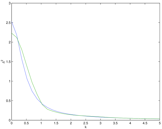
Figure 2: The propagator $\Delta^{2}(k)$, obtained by solving (40) at $\beta=3.0$ and $R=0.25$. The blue curve is the continued propagator. The green curve is reconstructed from the spectral density.

To obtain results for the spectral density we used the following prescription. First we continued the gap equations (70) – (74) to general Euclidean momenta, by writing, for example

$${\epsilon^{2}(k)\over\Delta^{2}(k)\epsilon^{2}(k)+\bigl{(}\gamma(k)\bigr{)}^{2}}=k^{2}+{4\over\beta}\sum_{l}\hat{\Delta}_{l}^{2}\epsilon^{2}\bigl{(}-k-{2\pi l\over\beta}\bigr{)}$$ (40)

$$\qquad\qquad\qquad\qquad+{4\over\beta}\sum_{l}\hat{\epsilon}_{l}^{2}\Delta^{2}\bigl{(}-k-{2\pi l\over\beta}\bigr{)}+{8\over\beta}\sum_{r}\hat{g}_{r}g\bigl{(}-k-{2\pi r\over\beta}\bigr{)}\,.$$

Then we obtained solutions to these equations for $R\geq 0.25$ at $\beta=2.0$, $3.0$, $4.0$. Below this value of $R$, and for larger values of $\beta$, it became difficult to obtain physical solutions to these equations. Fig. 2 shows the results of this procedure. By obtaining the propagators at frequencies intermediate to the Matsubara frequencies, we are able to obtain $\rho(\omega)$ with a much finer resolution than the spacing between Matsubara frequencies $2\pi/\beta$.

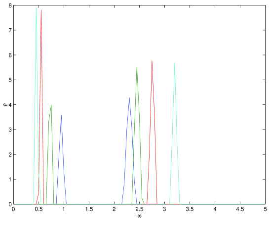
Figure 3: The spectral density $\rho(\omega)$ at $\beta=3.0$. Dark blue: $R=1.0$, green: $R=0.75$, red: $R=0.5$, light blue: $R=0.25$.

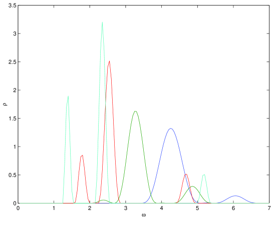
Figure 4: The spectral density $\rho(\omega)$ at $\beta=3.0$. Dark blue: $R=4.0$, green: $R=3.0$, red: $R=2.0$, light blue: $R=1.5$.

Finally, to reconstruct the spectral densities, we used a constrained Tikhonov regularization [17]. The essential idea is to numerically minimize a discretization of

$$\sum_{l}\left|\Delta^{2}_{l}-\int_{0}^{\infty}d\omega~{}\frac{\rho(\omega)}{(2\pi l/\beta)^{2}+\omega^{2}}\right|+\lambda^{2}\int d\omega\left|\frac{d\rho}{d\omega}\right|\,.$$ (41)

The minimization is performed subject to the constraint that $\rho\geq 0$. We also add terms corresponding to the constraints (38). The extra term dependent on the parameter $\lambda$ makes the matrices that appear in the inversion process well-conditioned. By choosing this extra term proportional to the norm of the derivative of $\rho$ we enforce smoothness of the solution, which helps to suppress numerical instabilities. We can actually choose this term to be quite small $\lambda=10^{-4}$, so that the contribution of the regulator to (41) is negligible. We should emphasize that no starting ansatz is needed to perform the minimization, so no prior knowledge about the final form of the solution is used as input, other than the features already mentioned. The spectral densities that result are shown in Figs. 3 and 4.

With this prescription, we believe we have obtained reliable results for the spectral density. The prescription seems to work best if the radius is not too large; the small peaks seen at large $\omega$ ($\omega\gtrsim 5$) in Fig. 4 may be numerical artifacts, since perturbative quantum mechanics predicts a single peak at large $R$. However the relative weight of these small high frequency peaks decreases as $R$ increases, consistent with perturbative expectations. More disturbing is the fact that the dominant peak appears to get wider at large $R$, in contrast to the perturbative result that there is a single peak which becomes sharper as $R$ increases. This behavior appears to be an artifact of the Tikhonov regularization. We have checked that the large $R$ propagators can be well-fit by a single Lorentzian spectral peak which becomes narrower as $R$ increases. As a check of our results, a comparison of the propagator reconstructed from the spectral density and the original mean-field propagator is shown in Fig. 2. The reason these do not agree more precisely is that we have imposed a positivity constraint on the spectral density. By only partially summing Feynman diagrams, we have preserved unitarity only approximately, so the spectral weight which would exactly reproduce the mean field propagator need not be positive. The reasonable agreement seen in Fig. 2 provides us with a good indicator for how well the mean field approximation is working.

Let us make some comments on the spectral densities we have obtained, neglecting the numerical artifacts which seem to be present for $\omega\gtrsim 5$. A striking feature of our results for the spectral density is a bimodal distribution of W masses at sufficiently small radii. The results of [5] indicate that the supergravity regime should correspond to approximately $R\leq 2$. At $R>2$ we find a single dominant peak in the spectral density, consistent with what is expected from the perturbative quantum mechanics. However as $R$ decreases below the scale where supergravity becomes a good approximation we find two peaks in the spectral density. This suggests that once we enter this regime, two different types of fundamental strings are contributing to the spectral weight. One set run between the probe brane and the black hole horizon. These become light as $R$ decreases, and account for the entropy of the black hole in the limit $R\to 0$. Another set of fundamental strings appear to run off to the strongly curved asymptotic region of the supergravity background. As can be seen from Fig. 3 the sum of the positions of the two peaks at a given $R$ is roughly $3.5$, independent of $R$. This is consistent with the above interpretation.

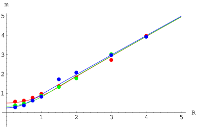
Figure 5: The lightest $W$ mass as a function of $R$ at $\beta=2.0$ (red), $\beta=3.0$ (green) and $\beta=4.0$ (blue).

A key feature of the spectral density is that a large number of light $W$ boson states are present when $R$ is small. We plot the lightest $W$ mass as a function of $R$ in Fig. 5 (we define this as the frequency $m_{W}$ which satisfies $\int_{0}^{m_{W}}d\omega\rho(\omega)=0.1$). At large $R$ we find $m_{W}\approx R$. As $R$ decreases $m_{W}$ also decreases. At some radius $m_{W}$ becomes of order the temperature and thermalization starts to occur. We identify this radius with the stretched horizon of the black hole. Note that the radius of the stretched horizon decreases with temperature, as expected.

Our reconstruction of the spectral density shows that the energy of the lightest W is approximately constant at small radius, for example at $\beta=3.0$ we find $m_{W}\approx 0.4$ for $R\lesssim 0.5$. This is compatible with the bound (39), which requires $m_{W}<0.51$ at $R=0$. This energy scale $m_{W}$ is indeed comparable to the temperature $1/\beta=0.33$. Thus absorption of the probe by the black hole can be understood as thermal restoration of $U(N+1)$ gauge symmetry.

5 Probe potential: reconstructing the spacetime metric from quantum mechanics

We wish to compare the probe free energy to the supergravity potential. To do this in a meaningful way, we must first determine how the supergravity radial coordinate $U$ is related to the Higgs expectation value $R$. The precise relationship can be obtained by comparing W masses, as follows.

Consider the mass of the lightest W boson in the quantum mechanics. At large $R$, where supersymmetry is restored and the quantum mechanics is weakly coupled, we can determine W masses perturbatively; a perturbative calculation gives $m_{W}=R+{\cal O}(1/R)$. As $R$ becomes small, however, the spectral analysis of the previous section indicates that the mass of the lightest W goes to a constant of order the Hawking temperature $T$. To find a useful analytic form that captures both these limits, we fit the lightest W mass to the following ansatz.

$$m_{W}=\left\{\begin{array}[]{ll}T+aR^{2}&\quad R<R_{0}\\ \vspace{2mm}\cr R+b/R&\quad R>R_{0}\end{array}\right.$$ (42)

Here $R_{0}$ is an adjustable parameter, while the constants $a$ and $b$ are fixed by demanding continuity of $m_{W}(R)$ and its first derivative at $R=R_{0}$. Fitting the ansatz to the data points shown in Fig. 5 yields the interpolating curves also shown there, with $R_{0}=1.5$ at $\beta=2.0$, $R_{0}=1.2$ at $\beta=3.0$, and $R_{0}=1.0$ at $\beta=4.0$.

On the other hand a supergravity computation of the W mass gives $m_{W}=(U-U_{0})/2\pi$ (11). This is the mass of a string which stretches from the probe to the horizon of the black hole. It seems appropriate to identify the mass of this string with the mass of the lightest W boson in the quantum mechanics. Thus we take the relation between $U$ and $R$ to be

$${U-U_{0}\over 2\pi}=\left\{\begin{array}[]{ll}T+aR^{2}&\quad R<R_{0}\\ \vspace{2mm}\cr R+b/R&\quad R>R_{0}\end{array}\right.$$ (43)

where $U_{0}$ is given by the supergravity relation (4). Of course this relation is only trustworthy in the region where supergravity makes sense, i.e. between the stretched horizon of the black hole and the region of large curvature $U\sim(g^{2}_{YM}N)^{1/3}$.

Let us make a few comments on this change of coordinates. Our results for the potential will not require the ansatz (43); we could invert the relation between $m_{W}$ and $R$ given by the data in Fig. 5, and express everything in terms of $m_{W}$. However one may wonder whether the ansatz (43) captures the correct functional relation between $U$ and $R$. Another functional form has been proposed in the literature [7, 18],

$$R^{7/2}={1\over 2}\left(\biggl{(}{U\over 2\pi}\biggr{)}^{7/2}+\sqrt{\biggl{(}{U\over 2\pi}\biggr{)}^{7}-\biggl{(}{U_{0}\over 2\pi}\biggr{)}^{7}}\right)\,.$$ (44)

This predicts that the relation

$$m_{W}={U-U_{0}\over 2\pi}={1\over R}\left(R^{7}+{1\over 4}\biggl{(}{U_{0}\over 2\pi}\biggr{)}^{7}\right)^{2/7}-{U_{0}\over 2\pi}$$

should hold in the supergravity regime. Suppose one makes an ${\cal O}(T)$ correction to this formula, and takes

$$m_{W}={1\over R}\left(R^{7}+{1\over 4}\biggl{(}{U_{0}\over 2\pi}\biggr{)}^{7}\right)^{2/7}-{U_{0}\over 2\pi}+T\,.$$ (45)

With $U_{0}$ regarded as an adjustable parameter, one can get a quite good fit to the data shown in Fig. 5. Within our numerical accuracy, we cannot claim to distinguish between the two proposals (43) and (45).

In Fig. 6 we show a plot of the probe free energy as a function of $R$, obtained by evaluating (35) at $\beta=3.0$. The continuous curve is the supergravity prediction for the effective potential (10). The $U$ coordinate is fixed using the relation (43) and the overall tension in the DBI action (8) is adjusted to fit the data. Note that we do not expect the overall coefficient to be accurately reproduced by the mean field approximation – in [5], where a complete mean-field calculation of the free energy of the background was performed, there was a $50\%$ discrepancy between the predicted coefficient and mean field, although the scaling exponent with temperature was reproduced to within a few percent. In our probe mean-field calculations we have not included the gauge multiplet or the 7^th scalar multiplet, and these fields are expected to make a substantial contribution to the overall coefficient.

Fig. 6 shows remarkable agreement for the shape of the potential. The $U$ vs. $R$ relation (43) is crucial in obtaining such good agreement. Because the supergravity effective potential depends in such a detailed way on the form of the black hole metric, we see that the mean field approximation in the quantum mechanics is accurately reproducing the spacetime physics of the black hole geometry.

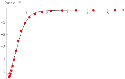
Figure 6: The probe free energy $\beta F$ vs. $R$, at $\beta=3.0$. The curve shows the Born-Infeld action (10) with the overall tension fit to the data.

One caveat is worth mentioning. The free energy of the probe (35) falls off like $1/R^{3}$ at large radius. This behavior is a consequence of the ${\cal N}=2$ supersymmetry of the truncated action (3.2). Note that supergravity has a potential (10) which falls off like $1/U^{7}$ far outside the horizon (at $U\gg U_{0}$). Thus with the truncation (3.2) we could not hope to see agreement with the long-distance behavior of supergravity. Fortunately, in the temperature range we are studying, the horizon radius $U_{0}$ is large enough that the shape of the supergravity effective potential is dominated by the square root singularity as $U\to U_{0}$. It is not particularly sensitive to whether $U^{7}$ appears or some other power of $U$ appears in the potential. This makes it possible for the truncated probe theory to reproduce well the shape of the potential.

Finally, let us discuss the behavior at small radius. The gauge theory has the property that as $R\rightarrow 0$ the probe 0-brane becomes indistinguishable from the $N$ 0-branes that make up the black hole background. This is clear from the form of the expectation value (16). This behavior is compatible with the properties of supergravity discussed at the end of section 2: the free energy of a probe that has come to equilibrium with the black hole can be obtained from the free energy of the background, simply by shifting $N\rightarrow N+1$.

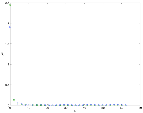
Figure 7: Comparison of the scalar propagators at small $R$ in the full mean field approximation (blue circles) and the truncated mean field approximation (green x’s), at $\beta=3.0$.

This behavior is respected by our approximation, in the sense that as $R\rightarrow 0$ the gap equations for the W propagators in the theory (31) become identical to the one-loop gap equations which we used to describe the black hole background in [5]. When we truncated the action, going from (31) to (3.2), we slightly violated the property that the background and W propagators agree at $R=0$. We can use this to test the validity of the truncation. A comparison of the scalar propagator at $R=0.1$ in our truncation, and the corresponding propagator for the background, is shown in Fig. 7. The zero frequency modes differ by about $20\%$, however this discrepancy rapidly decreases for the higher Matsubara modes: at $k=2\pi/\beta$ the difference is $9\%$, and becomes less than $1\%$ for $k\geq 14\pi/\beta$.

The free energy is rather more sensitive to the truncation than the propagators themselves. In the truncated probe mean field approximation we find $\beta F_{\rm probe}=-5.7$ as $R\rightarrow 0$ at $\beta=3.0$, whereas a complete mean-field calculation would give $\beta F_{\rm probe}=-2.0$ at $R=0$ (this follows from shifting $N\rightarrow N+1$ in the results of [5]). These free energies should be compared to the supergravity prediction $\beta F_{\rm probe}=-0.80$ for a probe in equilibrium with the black hole (13). We see that the full mean field is off by a factor of 2.5 from the supergravity prediction, while the truncated probe mean field is off by a factor of 7. The dominant source of the discrepancy between the two mean field results is the zero mode of the gauge field. The fact that the shape of the curves in Fig. 6 match so well suggests that the extra contribution due to the gauge zero mode leads only to a renormalization of the probe mass, and does not alter the overall shape of the potential. We plan to extend the probe mean field approximation to include the gauge multiplet, as well as the 7^th scalar multiplet, in future work. This will be important for seeing a more detailed matching of the probe mass, and also to resolve finer features of the probe effective potential.

6 Probe Entropy

We now turn to computing the entropy of the probe as a function of radius. Our expectation is that outside the stretched horizon, where supergravity is valid, the entropy of the probe should be very small. (In fact, according to classical supergravity, the entropy of the probe is exactly zero.) However as the probe reaches the stretched horizon light W’s become thermally excited, and the probe acquires a non-zero entropy. This should provide a clear signal for the breakdown of supergravity at the stretched horizon of the black hole.

We wish to compute the entropy of the probe while holding the mass of the black hole (and the radius of the probe) fixed. In the imaginary time formalism, the temperature of the probe is tied to the temperature of the black hole. This means we cannot compute the entropy using the canonical ensemble. Rather we have to define the probe entropy microcanonically. This is easily done, given the spectral representation (37). We merely have to integrate the spectral density against the entropy of a harmonic oscillator with frequency $\omega$ and temperature $1/\beta$

$$S_{\rm probe}=N\int d\omega\rho(\omega)\left({\beta\omega\over 2\tanh(\beta\omega/2)}-\log\bigl{(}2\sinh(\beta\omega/2)\bigr{)}\right)~{}.$$ (46)

The resulting entropy is shown in Fig. 8. (This is the entropy of a single W boson; to get the bosonic entropy of the full theory (3.2) one should multiply by 6). Of course there are also fermionic strings, which make an (additive) contribution to the total entropy, but the bulk of the entropy comes from the bosons.

We can see that the probe entropy is small at the edge of the eigenvalue cloud. For a spectral density of the sort we obtained in section 4, (46) predicts that the probe entropy is exponentially small outside the stretched horizon, roughly $S_{\rm probe}\sim e^{-\beta m_{W}}\sim e^{-\beta R}$. It only begins to increase dramatically at a considerably smaller radius, which we identify with the stretched horizon of the black hole. As can be seen in Fig. 8, the stretched horizon moves to smaller values of $R$ as the temperature decreases. Also note that the entropy increases more suddenly at lower temperatures. Both these features are in accord with the supergravity expectation (12).

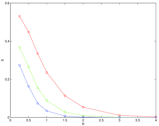
Figure 8: Bosonic contribution to the probe entropy vs. $R$ at $\beta=2.0$ (red), $\beta=3.0$ (green) and $\beta=4.0$ (blue). The edge of the eigenvalue distribution (17) lies at about $R=1.8$. Numerical calculations were performed at the indicated points.

7 An entropy – radius relation

As a final topic, we discuss an interesting relation between the entropy of a black hole and the radius of the black hole horizon. In this section we do not use a 0-brane probe, although much of what we will say is motivated by the results of the previous sections.

Within the context of our mean-field approximation [5], the black hole is modeled as a collection of $N^{2}$ independent degrees of freedom. Let $\rho(\omega)$ be the corresponding spectral density for the bosons. Then the entropy of the black hole is given by a formula analogous to (46),

$$S_{\rm bh}\sim N^{2}\int d\omega\rho(\omega)\left({\beta\omega\over 2\tanh(\beta\omega/2)}-\log\bigl{(}2\sinh(\beta\omega/2)\bigr{)}\right)$$ (47)

where we have neglected a small contribution from the fermions. The spectral density of the black hole background should be identical to the spectral density of a probe at very small radius. Having analyzed the probe spectral density, we expect that $\rho(\omega)$ has two peaks, one centered around $\omega\sim T$ and one centered around much higher frequencies. Moreover these peaks are very narrow. So up to a coefficient, the black hole entropy is just given by the area of the first low-frequency peak

$$S_{\rm bh}\sim N^{2}\int_{\hbox{\rm first peak}}d\omega\rho(\omega)~{}.$$ (48)

Now let us obtain an expression for the radius of the black hole horizon $R_{h}$. We will define this, not in terms of a probe brane, but rather as in section 5 of [5], in terms of the 2-point function of the time-averaged scalar fields (19). In terms of the spectral representation (36) we have

$$R_{h}^{2}\equiv\langle\bar{\phi}^{2}\rangle=\int_{0}^{\Lambda}d\omega\rho(\omega){1\over 2\omega\tanh(\beta\omega/2)}$$ (49)

where $\Lambda$ is a high-frequency cutoff, corresponding to a choice of resolving time used to define the size of the black hole. $\Lambda$ should be chosen to keep only the light modes, the modes which are described by supergravity. Since $\rho(\omega)$ has a bimodal distribution, there is a natural set of frequencies to exclude; we take the horizon size to be given by just integrating over the first low-frequency peak. As the peak is narrow and concentrated around $\omega\sim T$ we get (up to a numerical factor)

$$R_{h}^{2}\sim\beta\int_{\hbox{\rm first peak}}d\omega\rho(\omega)\,.$$ (50)

Combining (48) and (50) we get a non-trivial relationship between the horizon radius and entropy of the black hole. Restoring units

$$S_{\rm bh}\sim{N^{2}TR_{h}^{2}\over g^{2}_{YM}N}\,.$$ (51)

Note that we have obtained this relationship strictly within the gauge theory.

Remarkably, however, a supergravity relationship of this form is valid for all black holes that arise as the near-horizon geometry of black p-branes. The supergravity relationship is

$$S_{\rm bh}\sim{N^{2}TU_{0}^{2}\over g^{2}_{YM}N}$$ (52)

where the constant of proportionality depends on the dimension of the brane. This relationship was noticed in appendix C.2 of [4].

There are a few points worth mentioning about this derivation.

1. The gauge theory measures the horizon radius $R_{h}$ in terms of a Higgs field, while supergravity measures the horizon radius $U_{0}$ in terms of the radial coordinate $U$. The two coordinates are not the same. However in the range of temperatures we have studied, the two coordinates do not differ significantly. Also the considerations of [7, 18] suggest that $R_{h}$ is always proportional to $U_{0}$.

2. The expression (47) is only the leading expression for the entropy in the mean-field approximation. There is an infinite series of perturbative corrections to the leading mean-field result. As suggested in [4], these higher corrections may only change numerical coefficients, which we have anyways ignored.

We take the agreement between (51) and (52) to mean that the assumptions which went in to deriving (51) are qualitatively correct. In particular, this supports our claim that the spectral distribution has a clear separation of light and heavy degrees of freedom, and has a narrow peak at frequencies $\omega\sim T$.

8 Conclusions

In this paper we studied a 0-brane probe of a ten-dimensional non-extremal black hole, directly in terms of the dual strongly-coupled quantum mechanics. We described the black hole background using the mean-field methods of [5]. Following Susskind [15], we showed that a localized probe could be described in the quantum mechanics, once a suitable resolving time has been introduced. We studied the spectral representation of the W propagators, and found that light states are present in the quantum mechanics whenever the probe is inside the stretched horizon. These light states provide a mechanism for the black hole to absorb infalling matter, along the lines suggested in [11]. It would be quite interesting if these light states could be related to the light fractionated monopoles which Mathur proposed as an absorption mechanism for certain black holes [19].

Given the W propagators, it was straightforward to compute the free energy of the probe. We showed that outside the stretched horizon the probe potential was in accord with supergravity expectations. However the probe acquires a non-zero entropy once it enters the stretched horizon, as the light W states become thermally excited. This provides a clear signal that supergravity breaks down at the stretched horizon of a black hole, at least according to a Schwarzschild observer.

There are several interesting directions in which one could extend the results of this paper. For example, for simplicity we studied a truncated model for the probe (3.2), in which several fields were suppressed. But one can solve the full model (31), using essentially the same techniques. This should lead to improved results, in particular for the probe effective potential. Another interesting problem would be to study a probe with non-zero velocity. One could then compute, not only the probe potential, but also the probe kinetic terms. One could then hope to identify the non-trivial causal structure of the black hole metric (1), as reflected in the probe effective action (2).

Acknowledgements

We are grateful to Mike Douglas, Emil Martinec and Lenny Susskind for valuable discussions. NI and DK are supported by the DOE under contract DE-FG02-92ER40699. GL would like to thank Columbia University and Tel-Aviv University for hospitality. GL is supported in part by US–Israel binational science foundation grant 2000359. The research of DL is supported in part by DOE grant DE-FE0291ER40688 Task A.

Appendix A ${\cal N}=2$ superspace

With ${\cal N}=2$ supersymmetry we have an $SO(2)$ R-symmetry, with spinor indices $\alpha,\beta=1,2$ and vector indices $i,j=1,2$. The $SO(2)_{R}$ Dirac matrices $\gamma^{i}_{\alpha\beta}$ are real, symmetric, and traceless. Given two spinors $\psi$ and $\chi$, there are two invariants one can make, which we denote by

$$\psi_{\alpha}\chi_{\alpha}\qquad{\rm and}\qquad\psi^{\alpha}\chi_{\alpha}\equiv{i\over 2}\epsilon_{\alpha\beta}\psi_{\alpha}\chi_{\beta}\,.$$

${\cal N}=2$ superspace has coordinates $(t,\theta_{\alpha})$, where $\theta_{\alpha}$ is a collection of real Grassmann variables that transform as a spinor of $SO(2)_{R}$. The simplest representation of supersymmetry is a real scalar superfield (complex conjugation reverses the order of Grassmann variables)

$$\Phi=\phi+i\psi_{\alpha}\theta_{\alpha}+f\theta^{2}\,.$$

It contains a physical real boson $\phi$ and a physical real fermion $\psi_{\alpha}$, along with a real auxiliary field $f$. To describe gauge theory we introduce a real spinor connection on superspace $\Gamma_{\alpha}$, with component expansion

$$\Gamma_{\alpha}=\chi_{\alpha}+A_{0}\theta_{\alpha}+X^{i}\gamma^{i}_{\alpha\beta}\theta_{\beta}+d\epsilon_{\alpha\beta}\theta_{\beta}+2\epsilon_{\alpha\beta}\lambda_{\beta}\theta^{2}\,.$$

The fields $X^{i}$ are physical scalars, while $\lambda_{\alpha}$ are their superpartners, $d$ is an auxiliary boson, $\chi_{\alpha}$ are auxiliary fermions, and $A_{0}$ is the 0+1 dimensional gauge field.

To write a Lagrangian we introduce a supercovariant derivative

$$D_{\alpha}={\partial\over\partial\theta_{\alpha}}-i\theta_{\alpha}{\partial\over\partial t}$$ (53)

and its gauge-covariant extension

$$\nabla_{\alpha}=D_{\alpha}+\Gamma_{\alpha}\,.$$ (54)

The action for $N$ 0-branes is built from a collection of seven adjoint scalar multiplets $\Phi_{A}$ that transform in the ${\bf 7}$ of a $G_{2}\subset SO(9)$ global symmetry, coupled to a $U(N)$ gauge multiplet $\Gamma_{\alpha}$. The action reads

$$S={1\over g^{2}_{YM}}\int dtd^{2}\theta\,{\rm Tr}\biggl{(}-{1\over 4}\nabla^{\alpha}{\cal F}_{i}\nabla_{\alpha}{\cal F}_{i}-\frac{1}{2}\nabla^{\alpha}\Phi_{A}\nabla_{\alpha}\Phi_{A}-\frac{i}{3}f_{ABC}\Phi_{A}[\Phi_{B},\Phi_{C}]\biggr{)}\,.$$ (55)

Here ${\cal F}_{i}={1\over 4}\gamma^{i}_{\alpha\beta}\{\nabla_{\alpha},\nabla_{\beta}\}$ is the field strength constructed from $\Gamma_{\alpha}$, and $f_{ABC}$ is a totally antisymmetric $G_{2}$-invariant tensor, normalized to satisfy

$$f_{ABC}f_{ABD}={3\over 2}\delta_{CD}\,.$$ (56)

Appendix B Effective action and gap equations

The propagators (33) correspond to a Gaussian trial action for the off-diagonal fields (with a similar action for tilded fields)

$$S_{0}(\delta\Phi,\delta\Phi^{\dagger}) = \sum_{a,l}\left(\begin{array}[]{cc}\delta\phi_{{\bar{a}}l}^{\dagger}&\delta f_{{\bar{a}}l}^{\dagger}\end{array}\right)\left(\begin{array}[]{cc}\Delta_{l}^{2}&i\gamma_{l}\\ i\gamma_{l}&\epsilon_{l}^{2}\end{array}\right)^{-1}\left(\begin{array}[]{c}\delta\phi_{al}\\ \delta f_{al}\end{array}\right)$$ (68)

$$+i\sum_{a,r}\left(\begin{array}[]{cc}\delta\psi_{1{\bar{a}}r}^{\dagger}&\delta\psi_{2{\bar{a}}r}^{\dagger}\end{array}\right)\left(\begin{array}[]{cc}g_{r}&-h_{r}\\ h_{r}&g_{r}\end{array}\right)^{-1}\left(\begin{array}[]{c}\delta\psi_{1ar}\\ \delta\psi_{2ar}\end{array}\right)\,.$$

The 2-loop 2PI effective action discussed in [4, 5] is defined by

$$\beta F=\beta F_{0}+\langle S-S_{0}\rangle_{0}-{1\over 2}\langle(S_{III}^{2})\rangle_{{\hbox{\cmsss C}},0}$$

where $\beta F_{0}$ is the free energy of the trial action (68), $S-S_{0}$ is the difference between the full action (3.2) and the trial action (68), and $S_{III}$ refers to cubic terms in the full action. A subscript ${\hbox{\cmss C}},0$ denotes a connected expectation value computed using the trial action. In the present case, the effective action is given by

$$\beta F=-6N\sum_{l}\log\left(\Delta_{l}^{2}\epsilon_{l}^{2}+(\gamma_{l})^{2}\right)+6N\sum_{r}\log\left((g_{r})^{2}+(h_{r})^{2}\right)$$ (69)

$$+{6N\over g^{2}_{YM}}\sum_{l}\left(({2\pi l\over\beta})^{2}\Delta_{l}^{2}-2R\gamma_{l}+\epsilon_{l}^{2}-2g^{2}_{YM}\right)-{12N\over g^{2}_{YM}}\sum_{r}\left({2\pi r\over\beta}g_{r}-Rh_{r}-g^{2}_{YM}\right)$$

$$+{24N^{2}\over g^{4}_{YM}\beta}\sum_{l+m+n=0}\Delta_{l}^{2}\hat{\Delta}_{m}^{2}\epsilon_{n}^{2}+{12N^{2}\over g^{4}_{YM}\beta}\sum_{l+m+n=0}\Delta_{l}^{2}\hat{\epsilon}_{m}^{2}\Delta_{n}^{2}+{24N^{2}\over g^{4}_{YM}\beta}\sum_{l+m+n=0}\gamma_{l}\hat{\Delta}_{m}^{2}\gamma_{n}$$

$$+{48N^{2}\over g^{4}_{YM}\beta}\sum_{l+r+s=0}g_{r}\hat{g}_{s}\Delta_{l}^{2}+{24N^{2}\over g^{4}_{YM}\beta}\sum_{l+r+s=0}g_{r}\hat{\Delta}_{l}^{2}g_{s}-{24N^{2}\over g^{4}_{YM}\beta}\sum_{l+r+s=0}h_{r}\hat{\Delta}_{l}^{2}h_{s}~{}.$$

The effective action respects ’t Hooft large-$N$ scaling, so all factors of $g^{2}_{YM}N$ can be eliminated from (69) by appropriate rescalings of dimensionful quantities. For example, one sets

$$\beta=\beta^{\prime}/(g^{2}_{YM}N)^{1/3}\quad R=R^{\prime}(g^{2}_{YM}N)^{1/3}\quad\Delta_{l}^{2}=(g^{2}_{YM}N)^{1/3}\Delta^{\prime}_{l}{}^{2}/N\,.$$

The rescaled effective action, with the overall factor of $N$ suppressed, is given in (35). Requiring that the rescaled effective action is stationary with respect to variation of the propagators gives rise to the following set of gap equations

$${\epsilon_{l}^{2}\over\Delta_{l}^{2}\epsilon_{l}^{2}+(\gamma_{l})^{2}}=({\frac{2\pi l}{\beta}})^{2}+{4\over\beta}\sum_{m+n=-l}\hat{\Delta}_{m}^{2}\epsilon_{n}^{2}+{4\over\beta}\sum_{m+n=-l}\hat{\epsilon}_{m}^{2}\Delta_{n}^{2}+{8\over\beta}\sum_{r+s=-l}\hat{g}_{r}g_{s}$$

(70)

$${\Delta_{l}^{2}\over\Delta_{l}^{2}\epsilon_{l}^{2}+(\gamma_{l})^{2}}=1+{4\over\beta}\sum_{m+n=-l}\hat{\Delta}_{m}^{2}\Delta_{n}^{2}$$ (71)

$${\gamma_{l}\over\Delta_{l}^{2}\epsilon_{l}^{2}+(\gamma_{l})^{2}}=-R+{4\over\beta}\sum_{m+n=-l}\hat{\Delta}_{m}^{2}\gamma_{n}$$ (72)

$${g_{r}\over(g_{r})^{2}+(h_{r})^{2}}={\frac{2\pi r}{\beta}}-{4\over\beta}\sum_{l+s=-r}\hat{g}_{s}\Delta_{l}^{2}-{4\over\beta}\sum_{l+s=-r}\hat{\Delta}_{l}^{2}g_{s}$$ (73)

$${h_{r}\over(g_{r})^{2}+(h_{r})^{2}}=-R+{4\over\beta}\sum_{l+s=-r}\hat{\Delta}_{l}^{2}h_{s}~{}.$$ (74)

By comparing (71) and (72), note that $\gamma_{l}=-R\Delta_{l}^{2}$.

An important aid in finding numerical solutions to the gap equations is to solve for the large-momentum behavior of the propagators analytically [5]. At large momentum we find that the propagators have the behavior

$$\Delta_{l}^{2}\approx{1\over(2\pi l/\beta)^{2}+m_{\Delta}^{2}}\qquad\gamma_{l}\approx{-R\over(2\pi l/\beta)^{2}+m_{\gamma}^{2}}\qquad\epsilon_{l}^{2}\approx{(2\pi l/\beta)^{2}\over(2\pi l/\beta)^{2}+m_{\Delta}^{2}}$$

$$g_{r}\approx{2\pi r/\beta\over(2\pi r/\beta)^{2}+m_{\Delta}^{2}}\qquad h_{r}\approx{-R\over(2\pi r/\beta)^{2}+m_{h}^{2}}$$ (75)

where the asymptotic masses are given by

$$m_{\Delta}^{2} = R^{2}+{4\over\beta}\sum_{l}\hat{\Delta}_{l}^{2}+{4\over\beta}\sum_{l}\Delta_{l}^{2}$$ (76)

$$m_{\gamma}^{2} = R^{2}+{4\over\beta}\sum_{l}\hat{\Delta}_{l}^{2}+{8\over\beta}\sum_{l}\Delta_{l}^{2}+{4\over\beta R}\sum_{l}\gamma_{l}$$

$$m_{h}^{2} = R^{2}+{4\over\beta}\sum_{l}\hat{\Delta}_{l}^{2}+{8\over\beta}\sum_{l}\Delta_{l}^{2}+{4\over\beta R}\sum_{r}h_{r}\,.$$

References

-
[1]
O. Aharony, S. S. Gubser, J. Maldacena, H. Ooguri and Y. Oz,
Large N field theories, string theory and gravity,
Phys. Rept. 323, 183 (2000)
[hep-th/9905111];
T. Banks, TASI lectures on matrix theory, hep-th/9911068;
W. Taylor, M(atrix) theory: Matrix quantum mechanics as a fundamental theory, hep-th/0101126. - [2] N. Itzhaki, J. M. Maldacena, J. Sonnenschein and S. Yankielowicz, Supergravity and the large N limit of theories with sixteen supercharges, Phys. Rev. D 58, 046004 (1998) [hep-th/9802042].
-
[3]
S. Paban, S. Sethi and M. Stern,
Constraints from extended supersymmetry in quantum mechanics,
Nucl. Phys. B 534, 137 (1998)
[hep-th/9805018];
S. Paban, S. Sethi and M. Stern, Supersymmetry and higher derivative terms in the effective action of Yang-Mills theories, JHEP 9806, 012 (1998) [hep-th/9806028];
D.A. Lowe, Constraints on higher derivative operators in the matrix theory effective Lagrangian, [hep-th/9810075]. - [4] D. Kabat and G. Lifschytz, Approximations for strongly-coupled supersymmetric quantum mechanics, Nucl. Phys. B 571, 419 (2000) [hep-th/9910001].
-
[5]
D. Kabat, G. Lifschytz and D. A. Lowe,
Black hole thermodynamics from calculations in strongly-coupled gauge theory,
Phys. Rev. Lett. 86, 1426 (2001)
[hep-th/0007051];
D. Kabat, G. Lifschytz and D. A. Lowe, Black hole entropy from non-perturbative gauge theory, hep-th/0105171. -
[6]
S. Oda and F. Sugino,
Gaussian and mean field approximations for reduced Yang-Mills integrals,
JHEP 0103, 026 (2001)
[hep-th/0011175];
F. Sugino, Gaussian and mean field approximations for reduced 4D supersymmetric Yang-Mills integral, hep-th/0105284. - [7] J. Maldacena, Probing near extremal black holes with D-branes, Phys. Rev. D 57, 3736 (1998) [hep-th/9705053].
- [8] E. Kiritsis, Supergravity, D-brane probes and thermal super Yang-Mills: A comparison, JHEP 9910, 010 (1999) [hep-th/9906206].
- [9] I. R. Klebanov and A. A. Tseytlin, Entropy of Near-Extremal Black p-branes, Nucl. Phys. B 475, 164 (1996) [hep-th/9604089].
-
[10]
S. Rey, S. Theisen and J. Yee,
Wilson-Polyakov loop at finite temperature in large N gauge theory and anti-de Sitter supergravity,
Nucl. Phys. B 527, 171 (1998)
[hep-th/9803135];
A. Brandhuber, N. Itzhaki, J. Sonnenschein and S. Yankielowicz, Wilson loops in the large N limit at finite temperature, Phys. Lett. B 434, 36 (1998) [hep-th/9803137];
A. Brandhuber, N. Itzhaki, J. Sonnenschein and S. Yankielowicz, Wilson loops, confinement, and phase transitions in large N gauge theories from supergravity, JHEP 9806, 001 (1998) [hep-th/9803263]. -
[11]
D. Kabat and G. Lifschytz,
Tachyons and black hole horizons in gauge theory,
JHEP9812, 002 (1998)
[hep-th/9806214];
D. Kabat and G. Lifschytz, Gauge theory origins of supergravity causal structure, JHEP9905, 005 (1999) [hep-th/9902073]. - [12] E. Kiritsis and T. R. Taylor, Thermodynamics of D-brane probes, arXiv:hep-th/9906048.
- [13] M. Claudson and M. B. Halpern, Supersymmetric Ground State Wave Functions, Nucl. Phys. B 250, 689 (1985).
- [14] J. Polchinski, M-theory and the light cone, Prog. Theor. Phys. Suppl. 134, 158 (1999) [hep-th/9903165].
- [15] L. Susskind, Holography in the flat space limit, hep-th/9901079.
-
[16]
G. ’t Hooft,
A Two-Dimensional Model For Mesons,
Nucl. Phys. B 75, 461 (1974);
S. Coleman, Aspects of symmetry (Cambridge, 1985), chapter 8. - [17] A. N. Tikhonov and V. Y. Arsenin, Solutions of Ill-Posed Problems, Winston and Sons, Washington, D.C. 1977.
- [18] A. A. Tseytlin and S. Yankielowicz, Free energy of N = 4 super Yang-Mills in Higgs phase and non-extremal D3-brane interactions, Nucl. Phys. B 541, 145 (1999) [hep-th/9809032].
- [19] S. D. Mathur, Emission rates, the correspondence principle and the information paradox, Nucl. Phys. B 529, 295 (1998) [arXiv:hep-th/9706151].