ETH-TH/01-10 IEM-FT-217/01 CERN-TH/2001-202 hep-th/0108005
Finite Higgs mass without Supersymmetry

Abstract

We identify a class of chiral models where the one-loop effective potential for Higgs scalar fields is finite without any requirement of supersymmetry. It corresponds to the case where the Higgs fields are identified with the components of a gauge field along compactified extra dimensions. We present a six dimensional model with gauge group $U(3)\times U(3)$ and quarks and leptons accomodated in fundamental and bi-fundamental representations. The model can be embedded in a D-brane configuration of type I string theory and, upon compactification on a $T^{2}/{\mathbb{Z}}_{2}$ orbifold, it gives rise to the standard model with two Higgs doublets.

1 Introduction

In generic non-supersymmetric four-dimensional theories, the mass parameters of scalar fields receive quadratically divergent one-loop corrections. These divergences imply that the low-energy parameters are sensitive to contributions of heavy states with masses lying at the cut-off scale. Such expectations were confirmed by explicit computations in a string model in [1]. In fact, in the case where the theory remains four-dimensional up to the string scale $M_{s}\equiv l_{s}^{-1}$, we found that the string scale acts as a natural cut-off: the scalar squared masses are given by a loop factor times $M_{s}^{2}$ and the precise coefficient depends on the details of the string model.

However, in the case where some compactification radii are larger than the string length, which corresponds to the situation where, as energy increases, the theory becomes higher dimensional before the string scale is reached, we found a qualitatively different result. There, the one-loop effective potential was found to be finite and calculable from the only knowledge of the low energy effective field theory! For instance, in the five-dimensional case with compactification radius $R>l_{s}$, we found the scalar squared mass to be given by a loop factor times $1/R^{2}$, with exponentially small corrections. The precise factor is now completely determined by the low energy field theory.

The above behaviour can easily be understood from the fact that the scalar field considered in [1] corresponds to the component along the fifth dimension of a higher-dimensional gauge field [2]. The associated five-dimensional gauge symmetry protecting the scalar field from getting a five-dimensional mass is spontaneously broken by the compactification. As a result a four-dimensional mass term of order $1/R$ is allowed and gets naturally generated at one-loop.

In this work we would like to propose a scenario where the Higgs fields are identified with the internal components of a gauge field along TeV-scale extra-dimensions where the standard model gauge degrees of freedom can propagate [3, 4]. We will not present here a realistic model for fermion masses; instead, we would like to concentrate on the main properties of the electroweak symmetry breaking in an example and postpone a more realistic realization for a future work.

The adjoint representation of a gauge group containing the standard model Higgs, which is an electroweak doublet, should extend the electroweak gauge symmetry. The minimal extension compatible with the quantum numbers of the standard model fermion generations is $SU(3)\times SU(3)\times U(1)$. In this work, we construct a six-dimensional (6D) model with gauge group $U(3)\times U(3)$, which can be embedded in a D-brane configuration of type I string theory. It accomodates all quantum numbers of quarks and leptons in appropriate fundamental and bi-fundamental representations. The gauge group is broken to the standard model upon compactification on a $T^{2}/\mathbb{Z}_{2}$ orbifold, leaving as low energy spectrum the observable world with two Higgs doublets.

We would like to remind that many ingredients were already present in the literature. For instance, the identification of the Higgs field with an internal component of a gauge field is not new but a common feature of many string models. The use of this possibility in the case of large extra-dimension scenarios was already suggested in [4], where two standard model Higgs doublets were expected to arise from the orbifold action in six dimensions on $SU(3)$, in a way similar to the model we consider here. Moreover, there have been some proposals in various contexts of field theory where the Higgs field is identified with a gauge field component along extra dimensions, leading to finite one-loop mass in the case of smooth compactifications [2]. However, a further essential step was made in [1] as it was shown that embedding the higher dimensional theory in a string framework allows us to get a result for one-loop corrections that is calculable in the effective field theory. In order to obtain such a result from a field theory description it is necessary to assume that the theory contains an infinite tower of KK states and not a finite number truncated at the cut-off. The absence of ultraviolet divergences in the one-loop contribution to the Higgs mass when the whole tower of Kaluza-Klein (KK) excitations is taken into account has also been discussed by [5, 6, 7, 8]. However, in these cases supersymmetry was necessary in order to cancel the ultraviolet divergences in the loop contributions from bosonic (scalar and vector) and fermionic fields.

The content of this paper is as follows. In section 2 we derive the one-loop effective potential for a Higgs scalar identified with a continuous Wilson line. We show that the effective potential is insensitive to the ultraviolet cut-off in the case of toroidal compactification, and discuss the requirements in order to remain as such when performing an orbifold projection. In section 3 we study the minimization of this potential in the case of two extra dimensions. In section 4 we build a model with the representation content of the standard model from a compactification on a $T^{2}/\mathbb{Z}_{2}$ orbifold of a six-dimensional gauge theory. In section 5 we compute the one-loop Higgs mass terms for this model reproducing the results of sections 2 and 3. In section 6 we study the cancellation of anomalies in our model and obtain the induced corrections on the effective potential for the Higgs fields. Section 7 summarizes our results and discuss the requirements for more realistic models.

2 The one-loop effective potential

The four-dimensional effective potential for a scalar field $\phi$ is given by:

$$V_{eff}(\Phi)=\frac{1}{2}\sum_{I}(-)^{F_{I}}\int\frac{d^{4}p}{(2\pi)^{4}}\log\left[p^{2}+M_{I}^{2}(\phi)\right]\ .$$ (2.1)

where the sum is over all bosonic ($F_{I}=0$) and fermionic ($F_{I}=1$) degrees of freedom with $\phi$-dependent masses $M_{I}(\Phi)$. In the Schwinger representation, it can be rewritten as:

$$V_{eff}(\Phi) = -\frac{1}{2}\sum_{I}(-)^{F_{I}}\int_{0}^{\infty}\frac{dt}{t}\int\frac{d^{4}p}{(2\pi)^{4}}\,e^{-t\left[p^{2}+M_{I}^{2}(\phi)\right]}$$ (2.2)

$$= -\frac{1}{32\pi^{2}}\sum_{I}(-)^{F_{I}}\int_{0}^{\infty}\frac{dt}{t^{3}}\,\,e^{-tM_{I}^{2}(\phi)}$$ (2.3)

$$= -\frac{1}{32\pi^{2}}\sum_{I}(-)^{F_{I}}\int_{0}^{\infty}dl\,\,l\,\,e^{-{M_{I}^{2}(\phi)}/{l}}$$ (2.4)

where we have made the change of variables $t=1/l$. The integration regions $t\rightarrow 0$ ($l\rightarrow\infty$) and $t\rightarrow\infty$ ($l\rightarrow 0$) correspond to the ultraviolet (UV) and infrared (IR) limits, respectively.

We consider now the presence of $d$ (large) extra dimensions compactified on orthogonal circles with radii $R_{i}>1$ (in units of $l_{s}$) with $i=1,\dots,d$. The states propagating in this space appear in the four-dimensional theory as towers of KK modes of the $(4+d)$-dimensional states labeled by $I$ with masses given by:

$$M^{2}_{\vec{m},I}=M^{2}_{I}(\phi)+\sum_{i=1}^{d}\left[\frac{m_{i}+a^{I}_{i}(\phi)}{R_{i}}\right]^{2}$$ (2.5)

where ${\vec{m}}=\{m_{1},\cdots,m_{d}\}$ with $m_{i}$ integers. In (2.5) the term $M^{2}_{I}(\phi)$ is a $(4+d)$-dimensional mass which remains in the limit $R_{i}\rightarrow\infty$. The $(4+d)$-dimensional fields $\Psi_{I}$, whose Fourier modes decomposition along the $d$ compact dimensions have masses given by (2.5), satisfy the following periodicity conditions:

$$\Psi_{I}(x^{\mu},y^{i}+2\pi k_{i}R_{i})=e^{i2\pi\sum_{i}k_{i}a^{I}_{i}}\Psi_{I}(x^{\mu},y^{i})$$ (2.6)

where the $y^{i}$ coordinates parametrize the $d$-dimensional torus and $k_{i}$ are integer numbers. There are different cases where such a failure of periodicity appears and generates shifts $a^{I}_{i}$ for internal momenta. For instance, in the case of a Wilson line, $a^{I}_{i}=q^{I}\oint\frac{dy^{i}}{2\pi}gA_{i}$, where $A_{i}$ is the internal component of a gauge field with gauge coupling $g$ and $q^{I}$ is the charge of the $I$ field under the corresponding generator. Another case is when (2.6) appears as a junction condition, i.e. as a continuity condition of the wave function, in the presence of localized potential at $y^{i}=0$. In this work we will focus on the first situation.

The cases where $M^{2}_{I}(\phi)$ are independent of $\phi$ are of special interest. Such models, as we shall see shortly, lead to a finite one-loop effective potential for $\phi$. Here, we will consider for simplicity $M^{2}_{I}=0$, as a non-vanishing finite value would otherwise play the role of an infrared cut-off but does not introduce new UV divergences.

The effective potential obtained from (2.4) for the spectrum in (2.5) with $M^{2}_{I}=0$ is given by:

$$V_{eff}(\phi)|_{\rm torus}=-\sum_{I}\sum_{\vec{m}}(-)^{F_{I}}\frac{1}{32\pi^{2}}\int_{0}^{\infty}dl\,\,l\,\,e^{-\sum_{i}\frac{\left(m_{i}+a^{I}_{i}\right)^{2}}{R_{i}^{2}\,l}}$$ (2.7)

By commuting the integral with the sum over the KK states, and performing a Poisson resummation, the effective potential can be written as:

$$V_{eff}(\phi)|_{\rm torus}=-\sum_{I}(-)^{F_{I}}\,\frac{\prod_{i=1}^{d}R_{i}}{32\,\pi^{\frac{4-d}{2}}}\sum_{\vec{n}}e^{2\pi i\sum_{i}n_{i}a^{I}_{i}}\,\,\int_{0}^{\infty}dl\,\,l^{\frac{2+d}{2}}\,\,e^{-\pi^{2}l\sum_{i}n_{i}^{2}R_{i}^{2}}$$ (2.8)

The term with $\vec{n}=\vec{0}$ gives rise to a (divergent) contribution to the cosmological constant that needs to be dealt with in the framework of a full fledged string theory. This $\phi$-independent part is irrelevant for our discussion and can be forgotten. For all other (non-vanishing) vectors $\vec{n}\neq\vec{0}$ in (2.8), we make the change of variables: $l^{\prime}=\pi^{2}\,l\,\sum_{i}n_{i}^{2}R_{i}^{2}$ and perform the integration over $l^{\prime}$ explicitly. This leads to a finite result for the $\phi$-dependent part of the effective potential:

$$V_{eff}(\phi)|_{\rm torus}=-\sum_{I}(-)^{F_{I}}\,\,\frac{\Gamma(\frac{4+d}{2})}{32\pi^{\frac{12+d}{2}}}\,\,\prod_{i=1}^{d}R_{i}\,\,\sum_{\vec{n}\neq\vec{0}}\frac{e^{2\pi i\sum_{i}n_{i}a^{I}_{i}(\phi)}}{\left[\sum_{i}n_{i}^{2}R_{i}^{2}\right]^{\frac{4+d}{2}}}$$ (2.9)

These results call for a few remarks. A generic $(4+d)$-dimensional gauge theory is not expected to be consistent and its UV completion (the embedding in a consistent higher dimensional theory, as string theory) is needed. However we found that some one-loop effective potentials can be finite, computable in the field theory limit and insensitive to most of the details of the UV completion under the following conditions:

• One of the properties of the UV theory, we made use of, is to allow to sum over the whole infinite tower of KK modes. This was necessary in order to perform the Poisson resummation in (2.8). String theory provides an example with such a property. In the string embedding the effective potential (2.8) becomes:

  $$V_{eff}(\phi)|_{\rm torus}=-\sum_{I}(-)^{F_{I}}\,\frac{\prod_{i=1}^{d}\,R_{i}}{32\,\pi^{\frac{4-d}{2}}}\,\,\sum_{\vec{n}}e^{2\pi i\sum_{i}n_{i}a^{I}_{i}}\,\,\int_{0}^{\infty}dl\,\,l^{\frac{2+d}{2}}f_{s}(l)\,\,e^{-\pi^{2}l\sum_{i}n_{i}^{2}R_{i}^{2}}$$ (2.10)

  where $f_{s}(l)$ contains the effects of string oscillators. In the case of large radii $R_{i}>1$, only the $l\rightarrow 0$ region contributes. This means that the effective potential receives sizable contributions only from the IR (field theory) degrees of freedom. In this limit we should have $f_{s}(l)\rightarrow 1$. For example, in the model considered in [1]:

  $$f_{s}(l)=\left[\frac{1}{4l}\frac{\theta_{2}}{\eta^{3}}(il+{\frac{1}{2}})\right]^{4}\rightarrow 1\qquad{\rm for}\qquad l\rightarrow 0,$$ (2.11)

  and the field theory result (2.9) is recovered .

• A second, important, ingredient was the absence of a $(4+d)$-dimensional mass $M^{2}_{I}(\phi)$. The effective potential contains, for instance, a divergent contribution:

  $$V^{(\infty)}=\frac{1}{2}\sum_{I}(-)^{F_{I}}\,\int\frac{d^{4+d}p}{(2\pi)^{4+d}}\log\left[p^{2}+M^{2}_{I}(\phi)\right]\ .$$ (2.12)

  While this part identically cancels in the presence of supersymmetry, in a non-supersymmetric theory it usually gives a contribution to the $\phi$-dependent part of the effective potential which is sensitive to the UV physics introduced to regularize it. We will consider below the case where $\phi$ arises as a $(4+d)$-dimensional gauge field. The higher dimensional gauge symmetry will then enforce $M^{2}_{I}(\phi)=0$.

• Another issue is related with chirality. Compactification on tori is known to provide a non-chiral spectrum. Chiral fermions arise in more generic compactifications as orbifolds. These can be obtained from the above toroidal compactification by dividing by a discrete symmetry group. The orbifolding procedure introduces singular points, fixed under the action of the discrete symmetry, where new localized (twisted) matter can appear. These new states have no KK excitations along the directions where they are localized and they generically introduce, at one-loop, divergences regularized by the UV physics. To keep the one-loop effective potential finite, we need to impose that such localized states with couplings to $\phi$ are either absent or that they appear degenerate between bosons and fermions (supersymmetric representations).

The model of [1] discusses an explicit string example with the above properties.

Finally, we would like to comment on higher loop corrections. UV divergences are expected to appear at two loops, but they must be absorbed in one-loop sub-diagrams involving wave function renormalization counterterms. In other words the effect of two-loop divergences can be encoded in the running of gauge couplings [5, 8]. Then, requirement of perturbativity imposes that the string scale should not be hierarchically separated from the inverse compactification radius (not more than $\sim$ two orders of magnitude). An UV sensitive Higgs mass counterterm is not expected to appear at any order in perturbation theory because it is protected by the higher dimensional gauge invariance. On the other hand, in the presence of extra massless localized fields, there are two-loop diagrams depending logarithmically on the cutoff and leading to corrections to the Higgs mass proportional to $\log(M_{s}R)$ [9].

3 The six-dimensional case

In this section we would like to study in greater detail the case of two extra dimensions compactified on a torus.

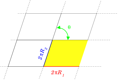
Figure 1: The two-dimensional torus

The torus is parametrized by the radii of the two non-contractible cycles $R_{1}$ and $R_{2}$ and the angle $\theta$ between the directions $x^{5}$ and $x^{6}$ (see Fig. 1). We will use the notation $\cos{\theta}=c$, $\sin{\theta}=s>0$. These parameters appear in the internal metric $G_{MN}$, $M,N=5,6$, the torus area $\sqrt{G}$ and the complex structure modulus $U$ given by:

$$G_{MN}=\left(\begin{array}[]{cc}R_{1}^{2}&R_{1}R_{2}c\\ R_{1}R_{2}c&R_{2}^{2}\end{array}\right);\qquad\sqrt{G}=R_{1}R_{2}s;\qquad U=\frac{R_{2}}{R_{1}}(c+is)$$ (3.3)

With this notation, the case of orthogonal circles corresponds to $\theta=\frac{\pi}{2}$, thus $c=0$. Instead of (2.5), the squared mass of the KK excitations now becomes:

$$M^{2}_{\vec{m},I} =\left|\frac{m_{2}+a_{2}-(m_{1}+a_{1})U}{\sqrt{Im\,U}G^{1/4}}\right|^{2}$$

$$=\frac{1}{s^{2}}\left[\frac{(m_{1}+a_{1})^{2}}{R_{1}^{2}}+\frac{(m_{2}+a_{2})^{2}}{R_{2}^{2}}-2\frac{(m_{1}+a_{1})(m_{2}+a_{2})c}{R_{1}R_{2}}\right]$$ (3.4)

where we assumed a vanishing six-dimensional mass $M^{2}_{I}(\phi)=0$.

Plugging the form (3.4) in the effective potential and performing a Poisson resummation, one can extract the part of the effective potential dependent on $a_{1}$ and/or on $a_{2}$ that takes the form:

$$V_{eff}(\phi)=-\sum_{I}(-)^{F_{I}}\,\,\frac{R_{1}R_{2}s}{16\pi^{7}}\,\,\sum_{\vec{n}\neq\vec{0}}\frac{\cos{[2\pi(n_{1}a_{1}+n_{2}a_{2})}]}{\left[n_{1}^{2}R_{1}^{2}+n_{2}^{2}R_{2}^{2}+2cn_{1}R_{1}n_{2}R_{2}\right]^{3}}$$ (3.5)

We consider here only the case where $a_{1}$ and $a_{2}$ are identified with Wilson lines:

$$a_{1}=\frac{1}{2\pi}q\oint gA_{5}dx^{5}\qquad a_{2}=\frac{1}{2\pi}q\oint gA_{6}dx^{6}$$ (3.6)

where the internal components $A_{5}$ and $A_{6}$ of a gauge field have constant expectations values in commuting directions of the associated gauge groups. Here $g$ is the gauge coupling and $q$ is the charge of the field circulating in the loop. In such a case the fields $a_{1}$ and $a_{2}$ have no tree-level potential and the one-loop contribution (3.5) represents the leading order potential for these fields.

The structure of the minima of the potential (3.5) determines the value of the compactification radii and torus angle $\cos\theta$ by imposing the correct EWSB scale at the minimum. For instance, in the case of one extra dimension the vacuum expectation value (VEV) at the minimum uniquely determines the compactification radius. It can be easily seen from (2.9) for $d=1$ that the minimum of the potential is at $a=1/2$ [1]. In any realistic model $a=m_{t}R$ where $m_{t}$ is the mass of the fermion which drives EWSB, i.e. the top in the case of standard model; thus it follows that $1/R=2m_{t}$ which is the result that was obtained in Ref. [7].

For the case we are considering here, $d=2$, the VEV at the minimum fixes one of the torus parameters while we have the freedom to fix the other two. In particular, if we restrict ourselves to the case of equal radii, i.e. $R_{1}=R_{2}\equiv R$, we can still consider the torus angle as a free parameter. Using torus periodicity and invariance under the orbifold action we can restrict the potential to the region $-1/2\leq a_{1},\,a_{2}\leq 1/2$. In fact the structure of the potential (3.5), symmetric with respect to $|a_{2}|\leftrightarrow|a_{1}|$, determines that, at the minimum $|a_{2}|=|a_{1}|\equiv a$.

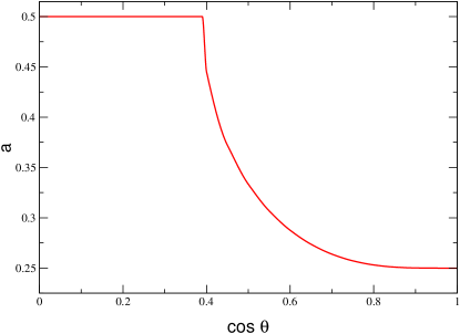
The minimum is plotted in Fig. 2 as a function of $\cos\theta$. We can see that for $\cos\theta<0.4$ the minimum is at $a=1/2$, which corresponds to $1/R=2m_{t}$. For $\cos\theta>0.4$ the minimum goes from $a=1/2$ to $a=1/4$, that would correspond to $1/R=4m_{t}\simeq 0.7$ TeV. Of course in the absence of a tree-level quartic term the corresponding Higgs mass would be below the experimental bounds and the model becomes non-realistic. We will discuss this issue in detail in section 6.

Figure 2: The minima of the effective potential (3.5), for $R_{1}=R_{2}$, as a function of $\cos\theta$.

4 A six-dimensional model

The $(4+d)$-dimensional Lagrangian for a Yang-Mills gauge field $A_{\hat{\mu}}$ coupled to a fermion $\Psi_{(4+d)}$ is given by :

$${\cal L}=-\frac{1}{2}\mathop{\rm Tr}F_{\hat{\mu}\hat{\nu}}F^{\hat{\mu}\hat{\nu}}-i\bar{\Psi}_{(4+d)}\Gamma^{\hat{\mu}}D_{\hat{\mu}}\Psi_{(4+d)}$$ (4.1)

where $\Gamma^{\hat{\mu}}$ represent the gamma matrices in $(4+d)$-dimensions. We use the metric: $\eta_{\hat{\mu}\hat{\nu}}={\rm diag}(-1,+1,\cdots,+1)$ and the notation $F_{\hat{\mu}\hat{\nu}}=\sum_{a}F^{(a)}_{\hat{\mu}\hat{\nu}}t_{a}$ and $A_{\hat{\mu}}=\sum_{a}A^{(a)}_{\hat{\mu}}t_{a}$ where the generators $t_{a}$ are normalised such that $\mathop{\rm Tr}\left(t_{a}t_{b}\right)=\delta_{ab}/2$. With this convention:

$$F_{\hat{\mu}\hat{\nu}} = \partial_{\hat{\mu}}A_{\hat{\nu}}-\partial_{\hat{\nu}}A_{\hat{\mu}}-ig\left[A_{\hat{\mu}}\,,\,A_{\hat{\nu}}\right]$$ (4.2)

$$D_{\hat{\mu}} = \partial_{\hat{\mu}}+igA_{\hat{\mu}}$$ (4.3)

where $g$ is the tree-level gauge coupling. Upon toroidal compactification the internal components $A_{M}$ of the gauge fields give rise to scalar fields. Some of them will be later identified with the standard model Higgs field so that the mass structure given in (2.5) is generated naturally. Furthermore, when the scalar fields are identified with the internal components $A_{M}$ of gauge fields, the higher dimensional gauge symmetry forbids the appearance of a $(4+d)$-dimensional mass term, i.e. $M^{2}_{I}(\phi)=0$.

Quartic couplings for the scalar fields are generated from the reduction to 4D of the quartic interaction among gauge bosons in 6D and takes the form:

$$V_{0}=\frac{g^{2}}{2}\sum_{M,N=5}^{d+4}Tr\left[A_{M},A_{N}\right]^{2}$$ (4.4)

The tree-level quartic interaction term is absent in the case of five-dimensional theory ($d=1$), leading to an unacceptably small Higgs mass ($\sim 50$ GeV). Therefore, a realistic model seems to require $d>1$. We discuss below the simplest example of $d=2$ extra dimensions.

We make the following choice of 6D $\Gamma$-matrices [10] satisfying the 6D Clifford algebra $\left\{\Gamma^{\hat{\mu}},\Gamma^{\hat{\nu}}\right\}=\,\eta^{\hat{\mu}\hat{\nu}}$:

$$\Gamma^{\mu}=\left[\begin{array}[]{ll}\gamma^{\mu}&0\\ 0&\gamma^{\mu}\end{array}\right];\qquad\Gamma^{5}=\left[\begin{array}[]{ll}0&-\gamma_{5}\\ \gamma^{5}&0\end{array}\right];\qquad\Gamma^{6}=\left[\begin{array}[]{ll}0&i\gamma_{5}\\ i\gamma_{5}&0\end{array}\right]$$ (4.11)

where $\gamma_{5}$ is the 4D gamma matrix satisfying $(\gamma_{5})^{2}=-1$. We can define the corresponding 6D Weyl projector:

$${\cal P}_{\pm}=\frac{1}{2}(1\pm i\Gamma^{7})=\left[\begin{array}[]{cc}\frac{1}{2}(1\mp i\gamma_{5})&0\\ 0&\frac{1}{2}(1\pm i\gamma_{5})\end{array}\right]$$ (4.14)

so that ${\cal P}_{+}$ and ${\cal P}_{-}$ leave invariant the positive and negative chiralities respectively. The 6D spinor $\Psi_{(6)}$ and the projectors can be written as:

$$\Psi_{(6)}=\left[\begin{array}[]{l}\psi_{+}\\ \psi_{-}\\ \Psi_{-}\\ \Psi_{+}\end{array}\right];\qquad{\cal P}_{+}=\left[\begin{array}[]{llll}1&0&0&0\\ 0&0&0&0\\ 0&0&0&0\\ 0&0&0&1\end{array}\right];\qquad{\cal P}_{-}=\left[\begin{array}[]{llll}0&0&0&0\\ 0&1&0&0\\ 0&0&1&0\\ 0&0&0&0\end{array}\right]$$ (4.27)

where $\psi_{\pm}$ and their mirrors $\Psi_{\pm}$ are (4D Weyl) two-component spinors. The eigenstates of ${\cal P}_{+}$ and ${\cal P}_{-}$ can be written as:

$$\Psi_{(6)+}=\left[\begin{array}[]{l}\psi_{+}\\ 0\\ 0\\ \Psi_{+}\end{array}\right]=\left[\begin{array}[]{l}\psi_{L}\\ 0\\ 0\\ \Psi_{R}\end{array}\right]\qquad\Psi_{(6)-}=\left[\begin{array}[]{l}0\\ \psi_{-}\\ \Psi_{-}\\ 0\end{array}\right]=\left[\begin{array}[]{l}0\\ \psi_{R}\\ \Psi_{L}\\ 0\end{array}\right]$$ (4.44)

where in the second equality we have dropped the 6D chirality indices and used the 4D chirality left (L) and right (R) indices.

We consider now a six-dimensional theory with gauge group $U(3)_{3}\times U(3)_{2}$ associated to two different gauge couplings $g_{3}$ and $g_{2}\equiv g$ respectively. This model can be embedded in a D-brane configuration of type I string theory containing two sets of three coincident D5-branes. The “color” branes give rise to $U(3)_{3}=SU(3)_{c}\times U(1)_{3}$ and contains the $SU(3)_{c}$ of strong interactions. Similarly, the “weak” branes give rise to $U(3)_{2}=SU(3)_{w}\times U(1)_{2}$ where $SU(3)_{w}$ contains the weak interactions. This is the smallest gauge group that allows to identify the Higgs doublet as component of the gauge field. Indeed, the adjoint representation of $SU(3)_{w}$ can be decomposed under $SU(2)_{w}\times U(1)_{1}$ as

$${\bf 8}={\bf 3}_{0}+{\bf 1}_{0}+{\bf 2}_{3}+{\bf{\bar{2}}}_{-3}\,,$$ (4.45)

where the subscripts are the charges under the $U(1)_{1}$ generator ${\cal Q}_{1}=\sqrt{3}\lambda_{8}$ with gauge coupling $g/\sqrt{12}$. We chose the normalization of the generators ${\cal Q}_{2}$ and ${\cal Q}_{3}$ of $U(1)_{2}$ and $U(1)_{3}$ such that the fundamental representation of $SU(3)_{i}$ has $U(1)_{i}$ charge unity [11]. The corresponding gauge couplings are then given by $g/\sqrt{6}$ and $g_{3}/\sqrt{6}$, respectively.

In addition to the gauge fields, the model contains three families of matter fermions in the representations

$$L_{1,2,3}=({\bf 1},{\bf 3})^{+}_{(0,1)},\qquad D^{\,c}_{1,2,3}=({\bf{\bar{3}}},{\bf 1})^{+}_{(-1,0)},$$ (4.46)

$$Q_{1}=({\bf 3},{\bf{\bar{3}}})^{+}_{(1,-1)}\qquad Q_{2}=({\bf 3},{\bf{\bar{3}}})^{-}_{(1,-1)}\qquad Q_{3}=({\bf{\bar{3}}},{\bf 3})^{-}_{(-1,1)}$$ (4.47)

where the notation $({\bf r_{3}},{\bf r_{2}})^{\epsilon}_{(q_{3},q_{2})}$ represents a six-dimensional Weyl fermion with chirality $\epsilon=\pm$ in the representations ${\bf r_{3}}$ and ${\bf r_{2}}$ of $SU(3)_{c}$ and $SU(3)_{w}$, respectively, and $U(1)$ charges $q_{3}$ and $q_{2}$ under the generators ${\cal Q}_{3}$ and ${\cal Q}_{2}$. The choice of the quantum numbers ensures the absence of all irreducible anomalies in six dimensions (see section 6).

In a D-brane configuration, the states $Q_{i}$ arise as fluctuations of open strings stretched between the color and weak branes. In contrast, the open strings giving rise to $L$ and $d^{\,c}$ need to have one end elsewhere as $L$ and $d^{\,c}$ carry charges only under one of the $U(3)$ factors. This requires the presence of another brane in the bulk, where we assume that the associated gauge group is broken at the string scale and is not relevant for our discussion. The details of the derivation of this model are presented in appendix A, along with two alternative possibilities of quantum number assignments that we do not use in this work.

As the six-dimensional chiral spinors contain pairs of left and right 4D Weyl fermions, the 6D model contains, besides the standard model states, their mirrors. Thus, the leptons appear as:

$$L_{L}=\left(\begin{array}[]{l}l\\ {\tilde{e}}\end{array}\right)_{L}\qquad\qquad{\rm and\,}\qquad\qquad L_{R}=\left(\begin{array}[]{l}{\tilde{l}}\\ e\end{array}\right)_{R}$$ (4.52)

while the quark representations are:

$$Q_{1,2L}=\left(\begin{array}[]{l}q\\ {\tilde{u}}\end{array}\right)_{L}\quad Q_{1,2R}=\left(\begin{array}[]{l}{\tilde{q}}\\ u\end{array}\right)_{R}\quad Q_{3L}=\left(\begin{array}[]{l}{\tilde{q}}^{c}\\ u^{c}\end{array}\right)_{L},\quad Q_{3R}=\left(\begin{array}[]{l}q^{c}\\ {\tilde{u}}^{c}\end{array}\right)_{R}$$ (4.61)

where $q$, $l$ are the quark and lepton doublets, and $u^{c}_{L}$, $d^{c}_{L}$, $e_{R}$ their weak singlet counterparts, while ${\tilde{q}}$, ${\tilde{l}}$, ${\tilde{u}}$ and ${\tilde{e}}$ are their mirror fermions.

To obtain a chiral 4D theory from the six dimensional model, we perform a $\mathbb{Z}_{2}$ orbifold:

$$x^{5}\rightarrow-x^{5}\qquad x^{6}\rightarrow-x^{6}$$ (4.62)

Each state can be represented as $|gauge>\otimes|spacetime>$ where $|gauge>$ represents the gauge quantum numbers (singlet, fundamental or adjoint representation of $U(3)$’s), while $|spacetime>$ represent the spacetime ones (scalar, vector or fermion). The orbifold acts on both of these quantum numbers.

The orbifold action on the spacetime quantum numbers is chosen to be:

$$\begin{array}[]{llll}{\rm even\,:}&A^{\mu}\rightarrow A^{\mu}&\qquad\qquad{\rm odd\,:}&A^{M}\rightarrow-A^{M}\end{array}\qquad M=5,\,6$$ (4.64)

The adjoint of $SU(3)$ is represented by $3\times 3$ matrices $t_{a}=\frac{\lambda_{a}}{2}$, where $\lambda_{a}$ are the well-known Gell-Mann matrices. The orbifold action on the adjoint representation of $U(3)_{2}$ is defined by:

$$t_{a}\rightarrow\Theta^{-1}t_{a}\Theta\,\qquad\qquad{\rm with\,}\qquad\Theta=\left(\begin{array}[]{lll}\,1&\,0&\,0\\ \,0&\,1&\,0\\ \,0&\,0&-1\end{array}\right)$$ (4.68)

As a result of combining the two actions, the invariant states from the adjoint representation of $U(3)_{3}$ are the 4D gauge bosons, while from the adjoint representation of $U(3)_{2}$ we obtain the $U(2)\times U(1)$ gauge bosons $A_{\mu}=\sum_{a=1,2,3,8}A^{(a)}_{\mu}\frac{\lambda_{a}}{2}+A^{(0)}_{\mu}\cdot\frac{\bf 1}{\sqrt{6}}$:

$$A_{\mu}=\frac{1}{2}\left(\begin{array}[]{ccc}\,W_{3}+\frac{1}{\sqrt{3}}\,A^{(8)}+{\sqrt{\frac{2}{3}}}A^{(0)}&\,{\sqrt{2}}{W^{+}}&\,0\\ \,{\sqrt{2}}{W^{-}}&\,-W_{3}+\frac{1}{\sqrt{3}}\,A^{(8)}+{\sqrt{\frac{2}{3}}}A^{(0)}&\,0\\ \,0&\,0&\frac{-2}{\sqrt{3}}\,A^{(8)}+{\sqrt{\frac{2}{3}}}A^{(0)}\end{array}\right)_{\mu}$$ (4.72)

(4.73)

as well as the scalar fields $H_{M}=\sum_{a=4,5,6,7}A^{(a)}_{M}\frac{\lambda_{a}}{2}$ where $M=5,6$. This takes the form:

$$H_{M}=\frac{1}{2}\left(\begin{array}[]{ccc}\,0&\,0&\,A^{(4)}_{M}+iA^{(5)}_{M}\\ \,0&\,0&\,A^{(6)}_{M}+iA^{(7)}_{M}\\ \,A^{(4)}_{M}-iA^{(5)}_{M}&\,A^{(6)}_{M}-iA^{(7)}_{M}&\,0\end{array}\right)=\frac{1}{2}\left(\begin{array}[]{lll}\,0&\,0&\,H_{M}^{+}\\ \,0&\,0&\,H_{M}^{0}\\ \,H_{M}^{-}&\,H_{M}^{0*}&\,0\end{array}\right)$$ (4.80)

It is useful to define $H=H_{5}-\gamma_{5}H_{6}$ :

$$H=\frac{1}{2}\left(\begin{array}[]{ccc}\,0&\,0&\,H_{5}^{+}-\gamma_{5}H_{6}^{+}\\ \,0&\,0&\,H_{5}^{0}-\gamma_{5}H_{6}^{0}\\ \,H_{5}^{-}-\gamma_{5}H_{6}^{-}&\,H_{5}^{0*}-\gamma_{5}H_{6}^{0*}&\,0\end{array}\right)=\left(\begin{array}[]{ccc}\,0&\,0&\,H_{2}^{+}\\ \,0&\,0&\,H_{2}^{0}\\ \,H_{1}^{-}&\,H_{1}^{0}&\,0\end{array}\right)$$ (4.87)

In addition, the orbifold projection acts on the fermions in the representation $r_{f}$ of $U(3)\times U(3)$ as:

$$\begin{array}[]{lllll}r_{f}\rightarrow\Theta r_{f}:&(1,3)_{L}&(3,{\bar{3}})_{L}&({\bar{3}},3)_{R}\\ r_{f}\rightarrow-\Theta r_{f}:&(1,3)_{R}&(3,{\bar{3}})_{R}&({\bar{3}},3)_{L}\\ r_{f}\rightarrow r_{f}:&({\bar{3}},1)_{L}&&&\\ r_{f}\rightarrow-r_{f}:&({\bar{3}},1)_{R}&&&\end{array}$$ (4.89)

leaving invariant, in the massless spectrum, just the standard model fields and projecting the mirrors away.

The model contains three $U(1)$ factors corresponding to the generators ${\cal Q}_{i}$ with $i=1,2,3$. As we will discuss in more details in section 6, there is only one anomaly free linear combination

$${\cal Q}_{Y} = \frac{{\cal Q}_{1}}{{6}}-\frac{2{\cal Q}_{2}}{3}-\frac{{\cal Q}_{3}}{3}$$ (4.90)

identified with the standard model hypercharge. The corresponding gauge coupling is given by:

$$\frac{1}{g_{Y}^{2}}=\frac{3}{g^{2}}+\frac{2}{3}\frac{1}{g_{3}^{2}}$$ (4.91)

which corresponds to a weak mixing angle $\theta_{w}$ (at the string scale) given by:

$$\sin^{2}{\theta_{w}}=\frac{1}{4+\frac{2}{3}\frac{g^{2}}{g_{3}^{2}}}$$ (4.92)

This relation coincides with one of the two cases considered in Ref. [11], which are compatible with a low string scale. Of course, a detailed analysis would need to be repeated in our model to take into account the change of the spectrum above the compactification scale.

The other two $U(1)$’s are anomalous. In a consistent string theory these anomalies are canceled by appropriate shifting of two axions. As a result the two gauge bosons become massive, giving rise to two global symmetries. One of them corresponding to ${\cal Q}_{3}$ is the ordinary baryon number which guarantees proton stability.

The projection on the fermions as chosen above leaves invariant only the standard model representations and projects away the mirror fermions from the massless modes. The low energy spectrum is then the standard model one with two Higgs doublets $H_{1}$ and $H_{2}$ as defined in (4.87).

The Higgs scalars have a quartic potential at tree level given in (4.4). As a function of the neutral components of the fields $H_{1}$ and $H_{2}$ the potential is given by :

$$V_{0}(H_{1}^{0},H_{2}^{0})=\frac{g^{2}}{2}\left(|H_{1}^{0}|^{2}-|H_{2}^{0}|^{2}\right)^{2}$$ (4.93)

which corresponds to the one of the minimal supersymmetric standard model with ${g^{\prime}}^{2}=3g^{2}$ due to the embedding of the hypercharge generator inside $SU(3)_{w}$ as given by (4.90).

The Higgs field coupling to fermions is given by:

$$-i\bar{\Psi}_{(4+d)}\Gamma^{M}D_{M}\Psi_{(4+d)}\rightarrow\bar{\Psi}_{(4+d)}\Gamma^{M}\left[-i\partial_{M}+g\sum_{a=4,5,6,7}A^{(a)}_{M}\frac{\lambda_{a}}{2}\right]\Psi_{(4+d)}$$ (4.94)

and leads to generation of fermion masses when the Higgs fields acquire VEVs.

5 One-loop Higgs mass

The Higgs scalars $H_{5}$ and $H_{6}$, or equivalently $H_{1}$ and $H_{2}$, arise as zero modes in the dimensional reduction of the six-dimensional gauge field on the torus. At tree level they are massless and have no VEV. However, as we will show here, at one-loop a (tachyonic) squared mass term can be generated inducing a spontaneous symmetry breaking. For simplicity, we will denote $H_{M}^{0}=H_{M}$ and $H_{M}^{0*}={\bar{H}}_{M}$ as they are the only components that will obtain a VEV. The generic mass terms for $H_{5}$ and $H_{6}$ are given by the coefficients of quadratic terms in the expansion of the effective Lagrangian around $H_{5}=H_{6}=0$,

$$-{\cal L}_{\rm mass} = M_{5{\bar{5}}}^{2}|H_{5}|^{2}+M_{6{\bar{6}}}^{2}|H_{6}|^{2}+M_{5{\bar{6}}}^{2}H_{5}{\bar{H}}_{6}+M_{{\bar{5}}6}^{2}{\bar{H}}_{5}H_{6}$$

$$= M_{5{\bar{5}}}^{2}|H_{5}|^{2}+M_{6{\bar{6}}}^{2}|H_{6}|^{2}+M_{+}^{2}(H_{5}{\bar{H}}_{6}+{\bar{H}}_{5}H_{6})+M_{-}^{2}(H_{5}{\bar{H}}_{6}-{\bar{H}}_{5}H_{6})\ ,$$

where we have defined:

$$M_{+}^{2}=\frac{1}{2}(M_{5{\bar{6}}}^{2}+M_{{\bar{5}}6}^{2})\qquad M_{-}^{2}=\frac{1}{2}(M_{5{\bar{6}}}^{2}-M_{{\bar{5}}6}^{2})$$ (5.2)

Reality of the Lagrangian (5) implies that $M_{\bar{5}5}$ and $M_{\bar{6}6}$ are real and $M_{\bar{5}6}=M_{\bar{6}5}^{*}$, so that $M_{+}^{2}$ is real, while $M_{-}^{2}$ is purely imaginary.

However, since the fields $H_{5,\,6}$ do not have a well defined hypercharge, we should write the Lagrangian for the standard model Higgs fields $H_{1,\,2}$. Using, from Eq. (4.87), $H_{5}=(\bar{H}_{1}+H_{2})/2$ and $H_{6}=(\bar{H}_{1}-H_{2})/2i$, this part of the Lagrangian can be written as a function of $H_{1}$ and $H_{2}$ as:

$$-{\cal L}_{\rm mass}=\,m_{1}^{2}\ |H_{1}|^{2}+m_{2}^{2}\ |H_{2}|^{2}+\mu_{+}^{2}\ (H_{1}H_{2}+{\bar{H}}_{1}\bar{H}_{2})+\mu_{-}^{2}\ (H_{1}H_{2}-{\bar{H}}_{1}\bar{H}_{2})$$ (5.3)

with

$$m_{1}^{2}=\frac{1}{4}\left[M_{5{\bar{5}}}^{2}+M_{6{\bar{6}}}^{2}\right]+i\ M_{-}^{2} m_{2}^{2}=\frac{1}{4}\left[M_{5{\bar{5}}}^{2}+M_{6{\bar{6}}}^{2}\right]-i\ M_{-}^{2}$$ (5.4)

$$\mu_{+}^{2}=\frac{1}{4}[M_{5{\bar{5}}}^{2}-M_{6{\bar{6}}}^{2}] \mu_{-}^{2}=i\ M_{+}^{2}$$ (5.5)

where $m_{1}^{2}$, $m_{2}^{2}$ and $\mu_{+}^{2}$ are real while $\mu_{-}^{2}$ is purely imaginary. The last two terms in (5.3) can be written in standard notation as $[m_{3}^{2}\,H_{1}H_{2}+h.c.]$ where $m_{3}^{2}=\mu_{+}^{2}+\mu_{-}^{2}$. If $\mu_{-}^{2}\neq 0$, $m_{3}^{2}$ is a complex parameter and there is explicit $CP$-violation if the phase of $m_{3}^{2}$ cannot be absorbed into a redefinition of the Higgs fields.

In general there can be one-loop generated quartic couplings, $\lambda_{5}$, $\lambda_{6}$ and $\lambda_{7}$, in the effective potential that can prevent such field redefinitions. They look like

$$-{\cal L}_{\rm quartic}=\frac{1}{2}\lambda_{5}(H_{1}H_{2})^{2}+(H_{1}\,H_{2})\left[\lambda_{6}\,|H_{1}|^{2}+\lambda_{7}\,|H_{2}|^{2}\right]+h.c.$$ (5.6)

However, in order to prevent tree-level flavor changing neutral currents one usually enforces the discrete $\mathbb{Z}_{2}$ symmetry, $H_{2}\to-H_{2}$, which is only softly violated by dimension-two operators, and prevents the appearance of $\lambda_{6}$ and $\lambda_{7}$-terms, i.e. $\lambda_{6}=\lambda_{7}=0$ [12]. In that case, the phase of $m_{3}^{2}$ cannot be absorbed into a redefinition of the Higgs fields provided that $Im(\lambda_{5}^{*}m_{3}^{4})\neq 0$, which signals $CP$-violation.

5.1 Toroidal compactification

We will first compute the Higgs mass parameters $M_{5{\bar{5}}}^{2}$, $M_{6{\bar{6}}}^{2}$, $M_{+}^{2}$ and $M_{-}^{2}$ induced at one-loop by the fermionic matter fields in the case of a compactification on a torus. We denote by $G_{IJ}$ the torus metric as given in (3.3) and by $G^{IJ}$ its inverse. The interaction Lagrangian between the six-dimensional Weyl fermion $\Psi_{\epsilon}$, satisfying ${\cal P}_{\epsilon}\Psi_{\epsilon}=\Psi_{\epsilon}$ with $\epsilon=\pm$, with the Higgs fields:

$$-g\bar{\Psi}_{\epsilon}\Gamma^{M}H_{M}\Psi_{\epsilon}$$ (5.7)

induces, at one-loop, a quadratic term $H_{I}\bar{H}_{J}$ from the diagram of Fig. 3.

Figure 3: One-loop diagram contributing to $M_{I{\bar{J}}}^{2}$.

Calculation of the diagram of Fig. 3 yields the result:

$$M^{2}_{I\bar{J}} = g^{2}\sum_{{p}^{5},\,{p}^{6}}\int\frac{d^{4}p}{(2\pi)^{4}}{\mbox{\rm Tr}}\left\{\Gamma^{I}\,{\cal P}_{\epsilon}\,\frac{1}{\hbox to0.0pt{$P$\hss}\hskip 1.29167pt/}\,\,\Gamma^{J}\,{\cal P}_{\epsilon}\,\frac{1}{\hbox to0.0pt{$P$\hss}\hskip 1.29167pt/}\,\right\}$$ (5.8)

$$= -4\,g^{2}\,R_{I}R_{J}\sum_{{p}^{5},\,{p}^{6}}\int\frac{d^{4}p}{(2\pi)^{4}}\left\{\frac{G^{IJ}}{p^{2}+p_{M}G^{MN}p_{N}}-\frac{2G^{IK}G^{JL}{p}_{K}{p}_{L}}{(p^{2}+p_{M}G^{MN}p_{N})^{2}}\right\}$$

with $\hbox to0.0pt{$P$\hss}\hskip 1.29167pt/=\Gamma_{\hat{\mu}}P^{\hat{\mu}}=\hbox to0.0pt{$p$\hss}\hskip 1.29167pt/+\Gamma_{5}p^{5}+\Gamma_{6}p^{6}$ where $p$ is the four-dimensional momentum. For simplicity of notations we use here $R_{5}\equiv R_{1}$ and $R_{6}\equiv R_{2}$. The $R_{I}R_{J}$ factors arise because the normalization of the metric is such that the $p^{I}$ are integers. In the last equality of (5.8) we have used the $\Gamma$-matrices property:

$${\mbox{\rm Tr}}\left[\Gamma^{I}{\cal P}_{\epsilon}\Gamma^{\hat{\mu}}\Gamma^{J}{\cal P}_{\epsilon}\Gamma^{\hat{\nu}}\right]=\frac{1}{2}{\mbox{\rm Tr}}\left[\Gamma^{I}\Gamma^{\hat{\mu}}\Gamma^{J}\Gamma^{\hat{\nu}}\right]=4(g^{I\hat{\mu}}g^{J\hat{\nu}}+g^{I\hat{\nu}}g^{J\hat{\mu}}-g^{IJ}g^{\hat{\mu}\hat{\nu}})$$ (5.9)

where $g^{\hat{\mu}\hat{\nu}}$ has elements $\{g^{\mu\nu}=\eta^{\mu\nu},g^{\mu I}=0,g^{IJ}=G^{IJ}R_{I}R_{J}\}$ .

Note that the result of (5.8) is independent of the six-dimensional chirality so we can choose $\epsilon=+$ without loss of generality.

To perform the integration in (5.8) we use the Schwinger representation:

$$\frac{1}{(p^{2}+m^{2})^{n}}=\frac{1}{\Gamma(n)}\int_{0}^{\infty}dt\,\,t^{n-1}\,\,e^{-(p^{2}+m^{2})t}$$ (5.10)

and make the change of variables $t=1/l$. This gives:

$$M^{2}_{I{\bar{J}}}=-\frac{4g^{2}}{16\pi^{2}}R_{I}R_{J}\sum_{p_{5},\,p_{6}}\int_{0}^{\infty}dl\,\,\,\,\left(G^{IJ}-\frac{2\,G^{IK}G^{JL}{p}_{K}{p}_{L}}{l}\right)\,\,e^{-(p_{M}G^{MN}p_{N})/2l}$$ (5.11)

As the momenta $p_{5}$ and $p_{6}$ take integer values, we can perform a Poisson ressumation which gives:

$$M^{2}_{I{\bar{J}}}=-\frac{4g^{2}\pi}{8}\sqrt{G}R_{I}R_{J}\sum_{{\tilde{p}}^{5},\,{\tilde{p}}^{6}}\int_{0}^{\infty}dl\,\,\,l^{2}\,\,\,{\tilde{p}}^{I}{\tilde{p}}^{J}\,\,\,e^{-\pi^{2}({\tilde{p}}^{M}G_{MN}{\tilde{p}}^{N})l}$$ (5.12)

where ${\tilde{p}}_{I}$ are momenta on the dual lattice. ${\tilde{p}}_{I}$ take integer values with our choice for the metric in (3.3). Notice that the integrand dies exponentially when $l\to\infty$ except when ${\tilde{p}}^{5}={\tilde{p}}^{6}=0$. However this term is zero in the summation (5.12) because of the prefactor ${\tilde{p}}^{I}{\tilde{p}}^{J}$ and the integral is well behaved for all values of ${\tilde{p}}^{5},\,{\tilde{p}}^{6}$. We finally make the change of variables $l^{\prime}=\pi^{2}({\tilde{p}}^{M}G_{MN}{\tilde{p}}^{N})l$ and perform the integration on $l^{\prime}$ to obtain:

$$M^{2}_{I\bar{J}}=-\frac{N_{F}g^{2}}{4\pi^{5}}\sqrt{G}\sum_{{\tilde{p}}^{5},\,{\tilde{p}}^{6}}\frac{R_{I}R_{J}{\tilde{p}}^{I}{\tilde{p}}^{J}}{\left[{\tilde{p}}^{M}G_{MN}{\tilde{p}}^{N}\right]^{3}}$$ (5.13)

with $N_{F}=4$ being the number of degrees of freedom of a six-dimensional Weyl spinor.

This corresponds to the mass parameters:

$$M_{5{\bar{5}}}^{2} = -\frac{N_{F}g^{2}}{4\pi^{5}}R_{1}R_{2}s\sum_{n_{1},\,n_{2}}\frac{n_{1}^{2}R_{1}^{2}}{\left[n_{1}^{2}R_{1}^{2}+n_{2}^{2}R_{2}^{2}+2c\,n_{1}n_{2}R_{1}R_{2}\right]^{3}},$$

$$M_{6{\bar{6}}}^{2} = -\frac{N_{F}g^{2}}{4\pi^{5}}R_{1}R_{2}s\sum_{n_{1},\,n_{2}}\frac{n_{2}^{2}R_{2}^{2}}{\left[n_{1}^{2}R_{1}^{2}+n_{2}^{2}R_{2}^{2}+2c\,n_{1}n_{2}R_{1}R_{2}\right]^{3}},$$

$$M_{+}^{2}=M_{5{\bar{6}}}^{2}=M_{{\bar{5}}6}^{2} = -\frac{N_{F}g^{2}}{4\pi^{5}}R_{1}R_{2}s\,\,\,\sum_{n_{1},\,n_{2}}\frac{n_{1}n_{2}\,R_{1}\,R_{2}}{\left[n_{1}^{2}R_{1}^{2}+n_{2}^{2}R_{2}^{2}+2c\,n_{1}n_{2}\,R_{1}R_{2}\right]^{3}}\ ,$$

$$M_{-}^{2} = 0\,$$ (5.14)

which implies that

$$m_{1}^{2}=m_{2}^{2} = -\frac{N_{F}g^{2}}{8\pi^{5}}R_{1}R_{2}s\sum_{n_{1},\,n_{2}}\frac{n_{1}^{2}R_{1}^{2}+n_{2}^{2}R_{2}^{2}}{\left[n_{1}^{2}R_{1}^{2}+n_{2}^{2}R_{2}^{2}+2c\,n_{1}n_{2}R_{1}R_{2}\right]^{3}},$$

$$\mu_{-}^{2} = -i\frac{N_{F}g^{2}}{4\pi^{5}}R_{1}R_{2}s\,\,\,\sum_{n_{1},\,n_{2}}\frac{n_{1}n_{2}\,R_{1}\,R_{2}}{\left[n_{1}^{2}R_{1}^{2}+n_{2}^{2}R_{2}^{2}+2c\,n_{1}n_{2}\,R_{1}R_{2}\right]^{3}}\ ,$$

$$\mu_{+}^{2} = 0\,$$ (5.15)

It is easy to check that the CP-violating term $\mu_{-}^{2}$ vanishes for $c=\cos{\theta}=0$. This yields $m_{3}^{2}$ purely imaginary so that if the quartic coupling $\lambda_{5}(H_{1}\,H_{2})^{2}+h.c.$ is generated with a real coefficient then $Im(m_{3}^{4}\,\lambda_{5}^{*})=0$ and there is no $CP$-violation.

5.2 Orbifold compactification

Let us now turn to the orbifold case of our example. We will carry the computation of the one-loop Higgs mass induced by the fermions originating from a six-dimensional Weyl fermion $\Psi_{+}$:

$$\Psi_{(6)+}=\left[\begin{array}[]{l}\psi_{L}\\ 0\\ 0\\ \Psi_{R}\end{array}\right]\qquad{\rm with\,}\qquad\psi_{L}=\left(\begin{array}[]{l}{\tilde{\phi}_{e}}\\ \phi_{e}\\ \phi_{o}\end{array}\right)\qquad{\rm and\,}\qquad\Psi_{R}=\left(\begin{array}[]{l}{\tilde{\bar{\chi}}_{o}}\\ {\bar{\chi}}_{o}\\ {\bar{\chi}}_{e}\end{array}\right)$$ (5.26)

The $\Gamma$-matrices $\Gamma^{\hat{\mu}}_{\perp}$ as written in (4.11) are given in an orthogonal basis. In order to write the Yukawa interaction with the Higgs fields we need to define the $\Gamma$-matrices in the basis associated to $x^{5},x^{6}$ and forming an angle $\theta$ (see Fig. 1):

$$\Gamma^{5} = \Gamma^{5}_{\perp}-\frac{c}{s}\ \Gamma^{6}_{\perp}$$

$$\Gamma^{6} = \frac{1}{s}\ \Gamma^{6}_{\perp}$$ (5.27)

which satisfy $\{\Gamma^{M},\Gamma^{N}\}=2g^{MN}$. The Yukawa interaction giving rise to masses for the components of the fermions in ${\cal L}$ can be obtained from the expansion of (5.7):

$${{\cal L}_{\rm Yukawa}} = -\,g\,\frac{1}{s}\,\left(H_{6}-e^{-i\theta}H_{5}\right)\,\,\,\bar{\phi_{e}}{\bar{\chi}}_{e}\,\,\,-\,g\,\frac{1}{s}\,\left({\bar{H}}_{6}-e^{i\theta}{\bar{H}}_{5}\right)\,\,\,{\chi}_{e}\phi_{e}$$ (5.28)

$$-\,g\,\frac{1}{s}\,\left({\bar{H}}_{6}-e^{-i\theta}{\bar{H}}_{5}\right)\,\,\,\bar{\phi_{o}}{\bar{\chi}}_{o}\,\,\,-\,g\,\frac{1}{s}\,\left(H_{6}-e^{i\theta}H_{5}\right)\,\,\,{\chi}_{o}\phi_{o}$$

As we are performing the computation in the symmetric phase, i.e. an expansion around $H_{M}=0$, we can use the free fields Kaluza-Klein decomposition of the fermion fields. The $\mathbb{Z}_{2}$-even states $\phi_{e}$ and ${\bar{\chi}}_{e}$ have the following decomposition:

$$\phi_{e} = \frac{1}{\pi\sqrt{R_{1}R_{2}}}\sum_{n_{1}=-\infty}^{\infty}\sum_{n_{2}=-\infty}^{\infty}\cos\left({\frac{n_{1}x^{5}}{R_{1}}}+{\frac{n_{2}x^{6}}{R_{2}}}\right)\phi^{(n_{1},n_{2})}_{e}$$

$${\bar{\chi}}_{e} = \frac{i}{\pi\sqrt{R_{1}R_{2}}}\sum_{n_{1}=-\infty}^{\infty}\sum_{n_{2}=-\infty}^{\infty}\cos\left({\frac{n_{1}x^{5}}{R_{1}}}+{\frac{n_{2}x^{6}}{R_{2}}}\right){\bar{\chi}}^{(n_{1},n_{2})}_{e}$$ (5.29)

while for the $\mathbb{Z}_{2}$-odd states $\phi_{o}$ and ${\bar{\chi}}_{o}$ we have,

$$\phi_{o} = \frac{1}{\pi\sqrt{R_{1}R_{2}}}\sum_{n_{1}=-\infty}^{\infty}\sum_{n_{2}=-\infty}^{\infty}\sin\left({\frac{n_{1}x^{5}}{R_{1}}}+{\frac{n_{2}x^{6}}{R_{2}}}\right)\phi^{(n_{1},n_{2})}_{o}$$

$${\bar{\chi}}_{o} = \frac{i}{\pi\sqrt{R_{1}R_{2}}}\sum_{n_{1}=-\infty}^{\infty}\sum_{n_{2}=-\infty}^{\infty}\sin\left({\frac{n_{1}x^{5}}{R_{1}}}+{\frac{n_{2}x^{6}}{R_{2}}}\right){\bar{\chi}}^{(n_{1},n_{2})}_{o}$$ (5.30)

where the transformation properties under the orbifold group action imply:

$$\phi^{(-n_{1},-n_{2})}_{e}=\phi^{(n_{1},n_{2})}_{e} \phi^{(-n_{1},-n_{2})}_{o}=-\phi^{(n_{1},n_{2})}_{o}$$

$${\bar{\chi}}^{(-n_{1},-n_{2})}_{e}={\bar{\chi}}^{(n_{1},n_{2})}_{e} {\bar{\chi}}^{(-n_{1},-n_{2})}_{o}=-{\bar{\chi}}^{(n_{1},n_{2})}_{o}$$ (5.31)

The Yukawa couplings of $H_{5}$ and $H_{6}$ are given by:

$$\int d^{4}x\int_{0}^{\pi R_{1}}dx^{5}\int_{0}^{\pi R_{2}}dx^{6}\left[gH_{5}\left(e^{-i\theta}\bar{\phi_{e}}{\bar{\chi}}_{e}+e^{i\theta}{\chi}_{e}\phi_{e}\right)-gH_{6}\left(\bar{\phi_{e}}{\bar{\chi}}_{e}+{\chi}_{e}\phi_{e}\right)\right]$$

(5.32)

while those of ${\bar{H}}_{5}$ and ${\bar{H}}_{6}$ can be obtained by complex conjugation. Using the KK-decomposition of (5.30) in (5.28) we obtain the coupling of $H_{6}$ to the KK-excitations of the fermion:

$${{\cal L}_{Y6}}=-\sum_{n_{1},\,n_{2}}\,\!\!\!^{\prime}\ igH_{6}\left({\bar{\phi}}^{(n_{1},n_{2})}_{e}{\bar{\chi}}^{(n_{1},n_{2})}_{e}+{\bar{\phi}}^{(n_{1},n_{2})}_{o}{\bar{\chi}}^{(n_{1},n_{2})}_{o}\right)+h.c.$$ (5.33)

where the summation $\sum\,\!\!^{\prime}$ is defined as,

$$\sum_{n_{1},\,n_{2}}\,\!\!\!^{\prime}\ \ f(n_{1},\,n_{2})=\sum_{n_{1}=1}^{\infty}\ \sum_{n_{2}=-\infty}^{\infty}\ f(n_{1},\,n_{2})+\sum_{n_{2}=0}^{\infty}\ f(0,\,n_{2})$$ (5.34)

Notice that there is no overcounting of states in (5.33) since, from (5.31), $\phi_{o}^{(0,0)}=\chi_{o}^{(0,0)}\equiv 0$. It is also important to note that even for this orbifold case the summation can be made on a full tower of KK-excitations $n_{1},n_{2}\in[-\infty,\infty]$. This can be made explicit by defining $\phi^{(n_{1},n_{2})}$ and $\chi^{(n_{1},n_{2})}$ through:

$$\phi^{(n_{1},n_{2})}=\left\{\begin{array}[]{ll}\phi^{(n_{1},n_{2})}_{e}&{\rm for}\ n_{1}>0\\ \phi^{(n_{1},n_{2})}_{e}&{\rm for}\ n_{1}=0,\,n_{2}>0\\ \phi^{(0,0)}_{e}&{\rm for}\ n_{1}=n_{2}=0\\ \phi^{(n_{1},n_{2})}_{o}&{\rm for}\ n_{1}=0,\,n_{2}<0\\ \phi^{(n_{1},n_{2})}_{o}&{\rm for}\ n_{1}<0\end{array}\right.,\ \chi^{(n_{1},n_{2})}=\left\{\begin{array}[]{ll}\chi^{(n_{1},n_{2})}_{e}&{\rm for}\ n_{1}>0\\ \chi^{(n_{1},n_{2})}_{e}&{\rm for}\ n_{1}=0,\,n_{2}>0\\ \chi^{(0,0)}_{e}&{\rm for}\ n_{1}=n_{2}=0\\ \chi^{(n_{1},n_{2})}_{o}&{\rm for}\ n_{1}=0,\,n_{2}<0\\ \chi^{(n_{1},n_{2})}_{o}&{\rm for}\ n_{1}<0\end{array}\right.$$ (5.45)

The interaction Lagrangian between $H_{6}$ and the fermions takes then the form:

$${\cal L}_{Y6}=-\sum_{n_{1}=-\infty}^{\infty}\sum_{n_{2}=-\infty}^{\infty}ig\left[H_{6}{\bar{\phi}}^{(n_{1},n_{2})}{\bar{\chi}}^{(n_{1},n_{2})}+{\bar{H}}_{6}{{\phi}}^{(n_{1},n_{2})}{{\chi}}^{(n_{1},n_{2})}\right]$$ (5.47)

The diagonal one-loop induced mass term $M_{6{\bar{6}}}^{2}|H_{6}|^{2}$ is then automatically finite, as it is due to a whole tower of KK states. In fact the contribution of a full tower can be computed directly from the toroidal case (5.13) with the replacement $N_{F}\rightarrow N_{F}({\rm orbifold})=\frac{1}{2}N_{F}({\rm torus})$.

In the same way, the Yukawa coupling of $H_{5}$ with fermions of positive six-dimensional chirality is given by:

$${{\cal L}_{Y5}}=\sum_{n_{1},\,n_{2}}\,\!\!\!^{\prime}\ gH_{5}\left[ie^{-i\theta}{\bar{\phi}}^{(n_{1},n_{2})}_{e}{\bar{\chi}}^{(n_{1},n_{2})}_{e}+ie^{i\theta}{\bar{\phi}}^{(n_{1},n_{2})}_{o}{\bar{\chi}}^{(n_{1},n_{2})}_{o}\right]+h.c.$$ (5.48)

When computing the one-loop diagrams of Fig. 3 contributing to $M_{5{\bar{5}}}^{2}$, the product of phases $e^{\pm i\theta}$ at the two vertices cancel to each other and the result also corresponds to the contribution of a whole tower of states. It can be obtained from $M_{6{\bar{6}}}^{2}$ through the exchange of $R_{1}$ with $R_{2}$. In fact, it is possible to write the Lagrangian (5.48) as a Yukawa coupling interaction of $H_{5}$ with a complete tower of KK excitations, as it was done in (5.47) for $H_{6}$, by making phase rotations on the fermions. However, for $\theta\neq\frac{\pi}{2}$ one cannot write simultaneously both (5.48) and (5.47) as interactions with a whole tower. In fact, the phase $e^{\pm i\theta}$ comes from the metric of the torus and for $\theta\neq\frac{\pi}{2}$ it is at the origin of the appearance of a $M_{-}^{2}$ term as we will see now.

The one-loop induced mixing terms between $H_{5}$ and $H_{6}$ can also be computed in a straightforward manner as the sum of the contribution of even states and that from odd states propagating in the loop of Fig. 3. The result of the one-loop mixing diagrams can be written formally as:

$$M_{5{\bar{6}}}^{2} = e^{-i\theta}\left(\begin{array}[]{l}{\rm contributions\,\,of}\\ {\rm\,\,even\,\,states}\end{array}\right)+e^{i\theta}\left(\begin{array}[]{l}{\rm contribution\,\,of}\\ {\rm\,\,odd\,\,states}\end{array}\right)$$ (5.53)

$$M_{{\bar{5}}6}^{2} = \,\,e^{i\theta}\left(\begin{array}[]{l}{\rm contribution\,\,of}\\ {\rm\,\,even\,\,states}\end{array}\right)+e^{-i\theta}\left(\begin{array}[]{l}{\rm contribution\,\,of}\\ {\rm\,\,odd\,\,states}\end{array}\right)$$ (5.58)

which implies:

$$M_{+}^{2}=c\left[\left(\begin{array}[]{l}{\rm contributions\,\,of}\\ {\rm\,\,even\,\,states}\end{array}\right)+\left(\begin{array}[]{l}{\rm contribution\,\,of}\\ {\rm\,\,odd\,\,states}\end{array}\right)\right]$$ (5.63)

$$M_{-}^{2}=-i\,\,s\left[\left(\begin{array}[]{l}{\rm contributions\,\,of}\\ {\rm\,\,even\,\,states}\end{array}\right)-\left(\begin{array}[]{l}{\rm contribution\,\,of}\\ {\rm\,\,odd\,\,states}\end{array}\right)\right]$$ (5.68)

In (5.63) the sum of contributions from even and odd states reproduces the one from a whole tower of states. The overall $c$ is necessary to reproduce the metric factor in the product of the two momenta $p_{5}$ and $p_{6}$ (see the double product in (5.8)). We then reproduce for $M_{+}^{2}$ the result of the torus with, again, $N_{F}\rightarrow N_{F}({\rm orbifold})=\frac{1}{2}N_{F}({\rm torus})$.

Next, we consider the mass parameter $M_{-}^{2}$. Due to the relative sign in (5.68), all the contributions of even and odd massive KK-states cancel to each other and only the divergent contribution of the massless mode remains! While each tower of KK excitations of the massless fermions contributes with a divergent result, the sum of all of these contributions is finite and, in our case, it vanishes. Indeed, the cancellation of irreducible non-abelian anomalies in six-dimensions (see next section) requires the fermions to arise from six-dimensional Weyl spinors that can be paired with opposite six-dimensional chiralities. While the Higgs field interaction with the positive chirality fermions is given by:

$${{\cal L}^{+}_{\rm Yukawa}}=-\,g\,\frac{1}{s}\,\left(H_{6}-e^{-i\theta}H_{5}\right)\,\,\,\bar{\phi_{e}}{\bar{\chi}}_{e}-\,g\,\frac{1}{s}\,\left(H_{6}-e^{i\theta}H_{5}\right)\,\,{\chi}_{o}\phi_{o}\,\,+h.c$$ (5.69)

the ones with negative chirality fermion interaction is given by

$${{\cal L}^{-}_{\rm Yukawa}}=-\,g\,\frac{1}{s}\,\left(H_{6}-e^{i\theta}H_{5}\right)\,\,\,\bar{\phi_{e}}{\bar{\chi}}_{e}-\,g\,\frac{1}{s}\,\left(H_{6}-e^{-i\theta}H_{5}\right)\,\,{\chi}_{o}\phi_{o}\,\,+h.c$$ (5.70)

The contribution of fermions originating from six-dimensional spinors with negative chirality can be obtained from the one due to spinors with positive chirality through the exchange of $e^{i\theta}\rightarrow e^{-i\theta}$. For each pair of such fermions the contribution to $M_{-}^{2}$ cancels. In our model of section 4, we have the leptons $L$ whose contribution is canceled by that of $Q_{3}$, and the quarks $Q_{2}$ that cancel the contributions from $Q_{1}$. The sum of the contributions of all fermions leads then to $M_{-}^{2}=0$.

Our results for the mass parameters are then:

$$N_{F} \rightarrow N_{F}({\rm orbifold})=\frac{1}{2}N_{F}({\rm torus})$$

$$M_{5{\bar{5}}}^{2} = -\frac{N_{F}g^{2}}{4\pi^{5}}R_{1}R_{2}s\sum_{n_{1},\,n_{2}}\frac{n_{1}^{2}R_{1}^{2}}{\left[n_{1}^{2}R_{1}^{2}+n_{2}^{2}R_{2}^{2}+2c\,n_{1}n_{2}R_{1}R_{2}\right]^{3}},$$

$$M_{6{\bar{6}}}^{2} = -\frac{N_{F}g^{2}}{4\pi^{5}}R_{1}R_{2}s\sum_{n_{1},\,n_{2}}\frac{n_{2}^{2}R_{2}^{2}}{\left[n_{1}^{2}R_{1}^{2}+n_{2}^{2}R_{2}^{2}+2c\,n_{1}n_{2}R_{1}R_{2}\right]^{3}},$$

$$M_{+}^{2}=M_{5{\bar{6}}}^{2}=M_{{\bar{5}}6}^{2} = -\frac{N_{F}g^{2}}{4\pi^{5}}R_{1}R_{2}s\,\,\,\sum_{n_{1},\,n_{2}}\frac{n_{1}n_{2}\,R_{1}\,R_{2}}{\left[n_{1}^{2}R_{1}^{2}+n_{2}^{2}R_{2}^{2}+2c\,n_{1}n_{2}\,R_{1}R_{2}\right]^{3}}\ ,$$

$$M_{-}^{2} = 0\,$$ (5.71)

which implies that

$$m_{1}^{2}=m_{2}^{2} = -\frac{N_{F}g^{2}}{8\pi^{5}}R_{1}R_{2}s\sum_{n_{1},\,n_{2}}\frac{n_{1}^{2}R_{1}^{2}+n_{2}^{2}R_{2}^{2}}{\left[n_{1}^{2}R_{1}^{2}+n_{2}^{2}R_{2}^{2}+2c\,n_{1}n_{2}R_{1}R_{2}\right]^{3}},$$

$$\mu_{-}^{2} = -i\frac{N_{F}g^{2}}{4\pi^{5}}R_{1}R_{2}s\,\,\,\sum_{n_{1},\,n_{2}}\frac{n_{1}n_{2}\,R_{1}\,R_{2}}{\left[n_{1}^{2}R_{1}^{2}+n_{2}^{2}R_{2}^{2}+2c\,n_{1}n_{2}\,R_{1}R_{2}\right]^{3}}\ ,$$

$$\mu_{+}^{2} = 0\,$$ (5.72)

It is important to note that results of the diagrammatic one-loop computation exactly reproduce the results of the expansion of the one-loop effective potential in section 3 upon identification: $H_{5}={\bar{H}_{5}}=a_{1}/gR_{1}$ and $H_{6}={\bar{H}_{6}}=a_{2}/gR_{2}$.

The geometrical origin of the mixing terms between $H_{5}$ and $H_{6}$ can be understood easily. Upon toroidal compactification, the six-dimensional Lorentz invariance is broken and one is left with translation invariance along the two internal dimensions. This symmetry is enough to forbid transitions between the components $A^{\prime}_{5}$ and $A^{\prime}_{6}$ of the internal gauge field in an orthogonal basis and thus forbids any mass term of the form $A^{\prime}_{5}A^{\prime}_{6}$. However, due to the presence of the angle $\theta\neq\frac{\pi}{2}$ the new fields $A_{6}$ have a component $cA_{6}$ along the fifth dimension, which implies transitions amplitudes between $A_{6}$ and $A_{5}$, or equivalently between $H_{5}$ and $H_{6}$, $c=\cos{\theta}\neq 0$. On the other hand, the mass terms $M_{-}^{2}$ ($\mu_{-}^{2}$) correspond to transitions between elements of the orthogonal basis which do not receive contributions from the bulk fields $M_{-}^{2}=\mu_{+}^{2}=0$. However, upon orbifolding of the torus, the translation invariance is broken at the boundaries and then terms mixing $A^{\prime}_{5}$ and $A^{\prime}_{6}$ could a priori appear localized on the fixed points through higher loops involving localized states.

6 Higgs potential from $U(1)$ anomaly cancellation

It is easy to show that the six-dimensional model with the spectrum given in (4.47) is free from irreducible anomalies . Indeed the associated anomaly polynomial which describes all mixed non-abelian and gravitational anomalies is factorizable and it is given by:

$$A_{6D}={\mbox{\rm tr}}{F_{c}^{2}}\,{\mbox{\rm tr}}{F_{w}^{2}}$$ (6.1)

where $F_{c}$ and $F_{w}$ are the strength fields of the $SU(3)_{c}$ and $SU(3)_{w}$ gauge fields respectively. The reducible anomaly (6.1) can be canceled by a generalized Green-Schwarz mechanism [13].

The compactification to four dimensions on the $T^{2}/\mathbb{Z}_{2}$ orbifold considered in section 4 does not produce any non-abelian anomalies. The chiral spectrum obtained through the $\mathbb{Z}_{2}$ projection leads however to anomalies for the $U(1)$ factors. The mixed anomalies of the three $U(1)$’s with non-abelian factors are given by the matrix $[{\cal A}_{ai}]$:

$$[{\cal A}_{\alpha i}]=\left(\begin{array}[]{ccc}\,-{6}&-\frac{3}{2}&0\\ -{{3}}&-3&\frac{9}{2}\end{array}\right)$$ (6.4)

where ${\cal A}_{\alpha i}={\mbox{\rm tr}}({\cal Q}_{i}t^{2}_{\alpha})$ with $t_{1}$ and $t_{2}$ the generators of $SU(3)_{c}$ and $SU(2)_{w}$ respectively. It is easy to check that one $U(1)$ combination, corresponding to the hypercharge $U(1)_{Y}$:

$${\cal Q}_{Y}=\frac{1}{3}\left(\frac{1}{2}{\cal Q}_{1}-2{\cal Q}_{2}-{\cal Q}_{3}\right)$$ (6.5)

obtained in (4.90), is anomaly free while the two other orthogonal combinations of $U(1)$ factors

$${\cal Q}^{\prime} = \frac{1}{\sqrt{30}}(2{\cal Q}_{1}+{\cal Q}_{3})$$

$${\cal Q}^{\prime\prime} = \frac{1}{\sqrt{30}}({\cal Q}_{2}-2{\cal Q}_{3})$$ (6.6)

are anomalous. These anomalies can generally be canceled in two possible ways: (i) By the appearance of extra matter localized at the orbifold fixed points with the appropriate quantum numbers to cancel the anomalies; (ii) By a generalized Green-Schwarz mechanism.

Although, for simplicity, we will only consider below the second possibility, the former one could also be easily realized. For instance, if the model originates from D5-(anti)branes in type IIB orientifolds, then D3-(anti)branes should also be introduced because of the $\mathbb{Z}_{2}$ orbifold. Open strings with one end on these branes and the other on the $U(3)\times U(3)$ D5-branes would give rise to extra matter fields needed to cancel the $U(1)$ anomalies. As stated in section 2, a sufficient condition to keep the one-loop Higgs mass finite is that these localized states must appear in supermultiplets. In this case, the results for the one-loop Higgs potential obtained above remain unchanged.

A way to avoid the appearance of extra branes and matter, is by making the $\mathbb{Z}_{2}$ orbifold freely acting, combining for instance its action with a shift by half a compactification lattice vector. Our computation can be easily generalized for this case.

The generalized Green-Schwarz mechanism to cancel the above anomalies rests on the observation that if the model is obtained using a string construction there should exist two (Ramond-Ramond) axion fields $a^{\prime}$ and $a^{\prime\prime}$ which transform non-trivially under the $U(1)^{\prime}$ and $U(1)^{\prime\prime}$ gauge transformations in order to cancel the anomalies [14]. The couplings of these fields to the corresponding gauge fields, $B^{\prime}_{\mu}$ and $B^{\prime\prime}_{\mu}$ is given by the Lagrangian:

$${\cal L} =-\frac{1}{2}(\partial_{\mu}a^{\prime}+\lambda M_{s}B^{\prime}_{\mu})^{2}-\frac{1}{2}\sum_{k}(\partial_{\mu}a^{\prime\prime}+\lambda M_{s}B^{\prime\prime}_{\mu})^{2}$$ (6.7)

$$-\frac{1}{32\pi^{2}}\ \frac{a^{\prime}}{\lambda M_{s}}\ \sum_{a}k^{\prime}_{a}\ F^{(a)}_{\mu\nu}\tilde{F}^{(a)\mu\nu}-\frac{1}{32\pi^{2}}\ \frac{a^{\prime\prime}}{\lambda M_{s}}\ \sum_{a}\ k^{\prime\prime}_{a}\ F^{(a)}_{\mu\nu}\tilde{F}^{(a)\mu\nu}$$

where $\lambda$ is a parameter that depends on the string model and

$$k^{\prime}_{1}={\mbox{\rm tr}}\left({\cal Q}^{\prime}t^{2}_{1}\right)\qquad k^{\prime}_{2}={\mbox{\rm tr}}\left({\cal Q}^{\prime}t^{2}_{2}\right)\qquad k^{\prime\prime}_{1}={\mbox{\rm tr}}\left({\cal Q}^{\prime\prime}t^{2}_{1}\right)\qquad k^{\prime\prime}_{2}={\mbox{\rm tr}}\left({\cal Q}^{\prime\prime}t^{2}_{2}\right)$$ (6.8)

In order to cancel the phase from the fermionic determinant, the axions $a^{\prime}$ and $a^{\prime\prime}$ need to transform as:

$$\delta B^{\prime}_{\mu}=\partial_{\mu}\Lambda^{\prime},\quad\ \delta a^{\prime}=g\lambda M_{s}\Lambda^{\prime}\qquad{\rm and}\qquad\delta B^{\prime\prime}_{\mu}=\partial_{\mu}\Lambda^{\prime\prime},\quad\ \delta a^{\prime\prime}=g\lambda M_{s}\Lambda^{\prime\prime}$$ (6.9)

In the analysis of the modifications of the Higgs potential due to the use of a Green-Schwarz mechanism for cancelling the anomalies, it is necessary to make use of a basis for the $U(1)$ charges. A possible choice is to use $U(1)_{Y}$, $U(1)_{{\cal Q}^{\prime}}$ and $U(1)_{{\cal Q}^{\prime\prime}}$ such that the anomaly free combination ${\cal Q}_{Y}$ is made manifest. Instead, it is more convenient for our discussion to use $U(1)_{1}$ (${\cal Q}_{1}$) since the Higgs fields do not carry charges under the other two $U(1)$’s. In order to obtain the modification to the Higgs potential we assume that the theory is obtained as a truncation of a supersymmetric (“super-parent”) theory projecting away the $R$-symmetry odd gauginos, sleptons, squarks and Higgsinos while keeping the $R$-parity even states: gauge bosons, matter fermions and Higgs scalars. The tree-level Lagrangian can then be obtained by putting to zero the $R$-odd states. This way of describing the model as a truncation allows to obtain the modification for tree level Higgs potential easily. Indeed, this potential given in (4.93) arises in the super-parent model as the $D$-term potential. Its modification due to the cancellation of anomalies through the Green-Schwarz mechanism is well known, and given by:

$$\frac{g^{2}}{8}\left(|H_{1}^{0}|^{2}-|H_{2}^{0}|^{2}\right)^{2}+\frac{3\,g^{2}}{8}\left(|H_{1}^{0}|^{2}-|H_{2}^{0}|^{2}\right)^{2}$$

$$\rightarrow \frac{g^{2}}{8}\left(|H_{1}^{0}|^{2}-|H_{2}^{0}|^{2}\right)^{2}+\frac{3\,g^{2}}{8}\left(|H_{1}^{0}|^{2}-|H_{2}^{0}|^{2}+\xi\frac{\varphi}{\sqrt{G}}\right)^{2}$$ (6.10)

where $\xi$ is proportional to $\lambda$ and $\varphi$ is a scalar modulus blowing up the orbifold singularities; it is complexified with the axion $a^{\prime}$. The first term in (6.10) arises from the $D$ term of the $U(1)$ in the Cartan of $SU(2)_{w}$, which is free of anomalies, while the second one arises from the $D$ term of $U(1)_{1}$, with anomalies canceled by the Green-Schwarz mechanism. The presence of $\frac{1}{\sqrt{G}}$ in (6.10) is due to the absence of the $U(1)$ anomaly in the decompactification limit.

The leading terms in the expansion of the scalar potential in powers of $H_{1}$ and $H_{2}$ are then given by:

$$V_{\rm total}=V_{c}(\varphi,G_{IJ})+V_{0}(H_{1},H_{2},\varphi,G_{IJ})+\Delta V_{1}$$ (6.11)

where $V_{0}$ is the tree-level potential including the $U(1)$-anomaly, Eq. (6.10), and $\Delta V_{1}$ is the one-loop effective potential from bulk field loops, computed in previous sections. We do not minimize with respect to $\varphi$, the internal metric $G_{IJ}$ and other moduli, as their corresponding effective potential $V_{c}$ is unknown. Instead, we consider these moduli as given parameters of the theory and carry the minimization only with respect to $H_{1}$ and $H_{2}$.

We will start by analyzing the structure of $V_{0}$ as a function of the four real fields $A_{1}=A_{5}^{(6)}$, $A_{2}=A_{6}^{(6)}$, $B_{1}=A_{5}^{(7)}$ and $B_{2}=A_{6}^{(7)}$, in terms of which the neutral components of Higgs doublets are defined as,

$$H_{5} =A_{1}+i\,B_{1},\quad H_{1}=\left[A_{1}-B_{2}-i(A_{2}+B_{1})\right]/2$$

$$H_{6} =A_{2}+i\,B_{2},\quad H_{2}=\left[A_{1}+B_{2}-i(A_{2}-B_{1})\right]/2$$ (6.12)

The potential $V_{0}$ reads,

$$V_{0}=\alpha\,(B_{1}\,A_{2}-A_{1}\,B_{2})^{2}+\beta\,(B_{1}\,A_{2}-A_{1}\,B_{2}+\xi\frac{\varphi}{\sqrt{G}})^{2}$$ (6.13)

where $\alpha=g^{2}/8$ and $\beta={g^{\prime}}^{2}/8$. Notice that the VEVs of the $A_{I}$-fields are, after a trivial rescaling by $gR_{I}$, the Wilson line background we introduced in section 3. In that case, i.e. for $B_{I}\equiv 0$, the potential $V_{0}$ is just a constant provided by the anomaly.

Minimization with respect to $A_{I}$ and $B_{I}$ yields the condition for the corresponding VEVs, $\langle A_{I}\rangle=a_{I}$, $\langle B_{I}\rangle=b_{I}$

$$a_{1}\,b_{2}-b_{1}\,a_{2}=\kappa^{2},\quad\kappa^{2}=\frac{{g^{\prime}}^{2}}{g^{2}+{g^{\prime}}^{2}}\ \xi\frac{\varphi}{\sqrt{G}}$$ (6.14)

and the squared mass matrix at the minimum is given by:

$$\mathcal{M}^{2}=2\,(\alpha+\beta)\left[\begin{array}[]{cccc}b_{2}^{2}&-b_{1}\,b_{2}&-b_{2}\,a_{2}&a_{1}\,b_{2}\\ -b_{1}\,b_{2}&b_{1}^{2}&b_{1}\,a_{2}&-b_{1}\,a_{1}\\ -b_{2}\,a_{2}&b_{1}\,a_{2}&a_{2}^{2}&-a_{1}\,a_{2}\\ a_{1}\,b_{2}&-b_{1}\,a_{1}&-a_{1}\,a_{2}&a_{1}^{2}\end{array}\right]$$ (6.15)

where the VEVs $a_{I}$ and $b_{I}$ are subject to the condition (6.14). The matrix (6.15) has one non-vanishing mass eigenvalue, given by

$$M^{2}=\frac{g^{2}+{g^{\prime}}^{2}}{2}\,v^{2}\ ,$$ (6.16)

where $v^{2}\equiv|H_{1}|^{2}+|H_{2}|^{2}$, and three massless eigenvalues corresponding to three flat directions of the potential $V_{0}$. The mass eigenstates are

$$\widetilde{A}_{1}= -\frac{a_{1}}{b_{2}}\,A_{1}+B_{2}$$ (6.17)

$$\widetilde{A}_{2}= \ \frac{a_{2}}{b_{2}}\,A_{1}+B_{1}$$ (6.18)

$$\widetilde{B}_{1}= \ \frac{b_{1}}{b_{2}}\,A_{1}+A_{2}$$ (6.19)

$$\widetilde{B}_{2}= \ \frac{b_{2}}{a_{1}}\,A_{1}-\frac{b_{1}}{a_{1}}\,A_{2}-\frac{a_{2}}{a_{1}}\,B_{1}+B_{2}$$ (6.20)

where $\widetilde{A}_{1}$, $\widetilde{A}_{2}$ and $\widetilde{B}_{1}$ are the flat directions of $V_{0}$.

If we define the $\beta$-angle as $\tan\beta=|H_{2}|/|H_{1}|$, we can use the equation of minimum (6.14) to write,

$$\tan\beta=\sqrt{\frac{v^{2}+\kappa^{2}}{v^{2}-\kappa^{2}}}\ .$$ (6.21)

In particular, in the absence of anomaly $\xi=0$ and $\tan\beta=1$.

Of course, the latter result is based on the tree-level minimization condition (6.14) and radiative corrections, corresponding to the introduction of the potential $\Delta V_{1}$, can provide small corrections to it. In particular we can introduce just the radiative mass terms of (5.72) in the potential $\Delta V_{1}$, neglect the one-loop generated quartic couplings compared to the tree-level quartic potential, and assume that the determination of $\tan\beta$ from (6.14) is a good enough approximation. The effective potential, written as a function of $H_{1}$ and $H_{2}$ contains now a term as $\mu_{-}^{2}\,H_{1}\,H_{2}+h.c.$ where $\mu_{-}^{2}$ is purely imaginary as given in (5.72). In fact, if we define $\mu_{-}^{2}\equiv im_{3}^{2}$ we can absorb the phase $e^{i\pi/2}$ into the Higgs product $H_{1}\,H_{2}$ and, since $\lambda_{6}=\lambda_{7}=0$ in (6.11), our approximated potential does not contain any explicit $CP$-violation. Using now the $SU(2)$ gauge invariance in order to rotate one of the Higgs field VEVs on its real part, the remaining degrees of freedom are $|H_{1}|$, $|H_{2}|$ and a phase, whose VEV would signal spontaneous $CP$ breaking. However, since $\lambda_{5}=\lambda_{6}=\lambda_{7}=0$ in (6.11), it is easy to see that the dynamical phase is driven to zero. Minimization conditions imply now,

$$|H_{1}|^{2}-|H_{2}|^{2}+\kappa^{2}=\frac{4}{g^{2}+g^{\prime\,2}}\,\cot 2\beta\ m_{3}^{2}$$ (6.22)

which generalizes Eq. (6.14). In fact, in the absence of $U(1)$ anomalies, for $\xi=0$, Eq. (6.22) is only consistent for $\tan\beta=1$, in agreement with Eq. (6.21). In a sense Eq. (6.14) can be seen as the limit of (6.22) when $R_{I}\to\infty$. However, for finite radii Eq. (6.22) can be used, if $\tan\beta$ is approximately fixed by (6.21), to relate the compactification radii and the physical VEV of the Higgs fields $v^{2}=|H_{1}|^{2}+|H_{2}|^{2}$. We will do this for the case of equal radii, $R_{1}=R_{2}=R$, and an arbitrary torus angle $c\equiv\cos\theta$. 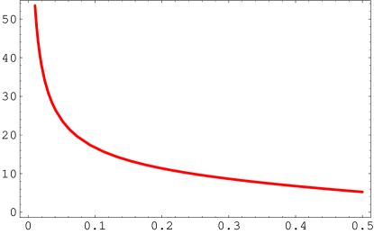Using the relations (6.22) and (5.72) we can write the compactification radius as a function of $c$ and the other parameters of the theory, as $v^{2}$, $\kappa^{2}$ and $\tan\beta$,

$$\frac{1}{R}=f(c)\ \sqrt{(10/N_{F})\left(v^{2}\sin 2\beta+\kappa^{2}\tan 2\beta\right)}\ .$$ (6.23)

We have arbitrarily normalized $N_{F}$ to 10 and the function $f(c)$, that can be easily obtained from (5.72), has been plotted in Fig. 4, where we have chosen $g^{2}=g^{\prime\,2}$.

Figure 4: The function $f(c)$ in (6.23).

From Fig. 4 we can see that, depending on the value of $c$, there is an enhancement factor for the compactification scale $1/R$ with respect to the weak scale $v$. This enhancement factor goes to $\infty$ when $c\to 0$ , which shows that we can obtain compactification scales larger than the weak scale $1/R\gg v$ for a range of torus angles. As we have seen in section 3 this enhancement factor disappears for pure Wilson lines since in that case the background field is along the direction $|H_{1}|=|H_{2}|$ and all quartic (non-radiative) contributions to the effective potential vanish.

7 Discussion

In this work we have studied the possibility that the standard model Higgs boson would be identified with the component of a gauge field along a compact extra dimension. The nice feature in such scenario is that the Higgs mass is expected to be free of one-loop quadratic divergences. Such divergences would introduce a mass to the Higgs field that would not vanish in the decompactification limit, and they are thus forbidden by the higher dimensional local gauge symmetry.

Although higher dimensional gauge theories are non-renormalizable, we have shown that for toroidal compactifications the full one-loop potential of the Higgs field can be explicitly computed without any reference to the underlying fundamental theory. As these toroidal compactifications do not lead to a chiral spectrum, it is necessary to introduce more complicated internal spaces. We considered here compactification on an orbifold obtained from the torus by gauging a discrete $\mathbb{Z}_{2}$ symmetry of the model. The finiteness of the one-loop Higgs mass is no more guaranteed in this case because of the presence of subspaces fixed under the orbifold where the local higher dimensional gauge symmetry is not conserved. Indeed, in existing string examples, one often obtains massless states localized at the orbifold fixed points in representations of the four dimensional (but not the higher dimensional) gauge group. We have shown that the one-loop result remains insensitive to the UV theory if the localized matter appears degenerate between fermions and bosons, forming $N=1$ supersymmetric multiplets. Such a situation appears for instance in the class of non-supersymmetric string models that were studied in [1].

For such orbifold models we have computed the one-loop Higgs mass, both from the analysis of the effective potential and from a diagrammatic one-loop computation, and shown to agree. The former method allows to compute the full one-loop effective potential dependence on tree-level flat directions. Instead, in the second (diagrammatic) approach we are able to compute the quadratic part for all scalar fields, however only as an expansion around the symmetric phase where the VEVs vanish.

In a fully realistic model the fermion flavor should be incorporated from the fundamental theory. In fact, as the Higgs is identified with an internal component of a gauge field, all tree level Yukawa couplings are given by the gauge coupling and all particles interacting with the Higgs field participate equally in generating its mass. This is to be contrasted with the usual case where the one-loop Higgs mass is dominated by the top quark due to the hierarchy of Yukawa couplings. A possible approach would be to identify the two light generations with (supersymmetric) boundary states with no tree level Yukawa couplings. In this work we did not attempt to address the problem of hierarchy of fermion masses. Instead, we tried to build a simple model from compactifications on orbifold in order to illustrate the main features of the scenario. We constructed a model where the massless representations are exactly the ones of the standard model, with two Higgs doublets originating from the internal components of a gauge field. It was obtained as a compactification of a six-dimensional model with gauge group $U(3)\times U(3)$ on a $T^{2}/\mathbb{Z}_{2}$ orbifold.

Appendix A Embedding of the standard model in $U(3)\times U(3)$

We will assume that the model can be embedded in a configuration of D-branes of type I strings. In such a case matter fields arise as massless fluctuations of open strings stretched between two sets of branes. Given $n$ sets of coincident $N_{i}$, $i=1,\cdots n$, D-branes, the associated gauge group is $U(N_{1})\times\cdots\times U(N_{n})\equiv SU(N_{1})\times\cdots\times SU(N_{n})\times U(1)_{N_{1}}\times\cdots\times U(1)_{N_{n}}$, with non-abelian gauge couplings $g_{N_{i}}$ and abelian ones normalized as $g_{N_{i}}/\sqrt{2N_{i}}$. An open string starting on one of the $N_{i}$ and ending on one of the $N_{j}$ branes transforms in the representation $(N_{i},{\bar{N_{j}}})$ of $SU(N_{i})\times SU(N_{j})_{(1,-1)}$ where $(1,-1)$ are the $U(1)_{N_{i}}\times U(1)_{N_{j}}$ charges.

For the purpose of embedding the standard model, we choose $n=2$ and $N_{1}=N_{2}=3$, so that the gauge group is $U(3)_{3}\times U(3)_{2}\equiv SU(3)_{c}\times SU(3)_{w}\times U(1)_{3}\times U(1)_{2}$. We denote by ${\cal Q}_{3}$ and ${\cal Q}_{2}$ the charges associated to $U(1)_{3}$ and $U(1)_{2}$, respectively. The weak $SU(3)_{w}$ contains $SU(2)_{w}\times U(1)_{1}$ as its maximal subgroup, with the generator ${\cal Q}_{1}$ of $U(1)_{1}$ represented in the adjoint of $SU(3)_{w}$ as $\sqrt{3}\lambda_{8}$. Here $\lambda_{8}$ is the diagonal Gell-Mann matrix with entries $\{1/\sqrt{3},1\sqrt{3},-2\sqrt{3}\}$.

The standard model hypercharge is a linear combination of the three $U(1)$ charges ${\cal Q}_{1}$, ${\cal Q}_{2}$ and ${\cal Q}_{3}$:

$${\cal Q}_{Y} = c_{1}{\cal Q}_{1}+c_{2}{\cal Q}_{2}+c_{3}{\cal Q}_{3}$$ (A.1)

where the coefficients $c_{i}$ are such that it reproduces the standard model representation quantum numbers.

First, note that the Higgs doublets arising from the decomposition of the adjoint of $SU(3)_{w}$ in irreducible representations of $SU(2)_{w}\times U(1)_{1}$ are not charged with respect to either ${\cal Q}_{2}$ or ${\cal Q}_{3}$. With their hypercharge normalized as $\pm 1/2$ we obtain $c_{1}=1/6$. Next, we consider the lepton doublets $l$ to arise from the representation $({\bf 1},{\bf 3})_{L}$, while the singlet $e_{R}$ belongs to the mirror representation $({\bf 1},{\bf 3})_{R}$. In order to obtain the correct normalization of the corresponding hypercharges, we are led to $c_{2}=-2/3$. Finally, for the quark representations we find two possible choices, corresponding to put either the $u^{c}$ or the $d^{c}$ quark with the quark doublet in the bifundamental representation of $SU(3)_{c}\times SU(3)_{w}$. The first choice leads to the model described in section 4. The other choice leads to $c_{3}=2/3$ with matter representations:

$$L_{1,2,3}=({\bf 1},{\bf 3})^{+}_{(0,1)},\qquad U_{1,2,3}=({\bf{3}},{\bf 1})^{+}_{(1,0)},$$ (A.2)

$$Q_{1}=({\bf 3},{\bf 3})^{-}_{(1,1)}\qquad Q_{2}=({\bf{3}},{\bf{3}})^{-}_{(1,1)}\qquad Q_{3}=({\bf{3}},{\bf{3}})^{+}_{(1,1)}$$ (A.3)

The standard model representations are obtained through a $\mathbb{Z}_{2}$ orbifold on the representations $r_{f}$ as:

$$\begin{array}[]{lllll}r_{f}\rightarrow\Theta r_{f}:&({\bf 1},{\bf 3})_{L}&({\bf 3},{\bf 3})_{L}\\ r_{f}\rightarrow-\Theta r_{f}:&({\bf 1},{\bf 3})_{R}&({\bf 3},{\bf 3})_{R}\\ r_{f}\rightarrow r_{f}:&({\bf 3},{\bf 1})_{R}&&&\\ r_{f}\rightarrow-r_{f}:&({\bf 3},{\bf 1})_{L}&&&\end{array}$$ (A.5)

which keeps the standard model fermions and projects the mirrors away. Only one linear combination is anomaly free and corresponds to the hypercharge

$${\cal Q}_{Y} = \frac{{\cal Q}_{1}}{{6}}-\frac{2{\cal Q}_{2}}{3}+\frac{2{\cal Q}_{3}}{3}$$ (A.6)

The corresponding tree-level gauge coupling is given by:

$$\frac{1}{g_{Y}^{2}}=\frac{3}{g^{2}}+\frac{8}{3}\frac{1}{g_{3}^{2}}$$ (A.7)

and corresponds to a weak mixing angle $\theta_{w}$ given by:

$$\sin^{2}{\theta_{w}}=\frac{1}{4+\frac{8}{3}\frac{g^{2}}{g_{3}^{2}}}$$ (A.8)

Note that both this model and the one presented in section 4 require the presence of a new brane where the open strings giving rise to $L$ and $D^{c}$ or $U$ will end. One way to avoid the introduction of the new brane is to make use of the fact that the representation ${\bf\bar{3}}$ can be obtained as the antisymmetric product of two ${\bf 3}$’s. $L$ and $D^{c}$ can then be identified with massless exitations of open strings with both ends on the weak and color D-branes, respectively, and corresponding $U(1)$ charges, $L=({\bf 1},{\bf 3})_{(0,2)}$ and $D^{c}=({\bf{\bar{3}}},{\bf 1})_{(-2,0)}$. The hypercharge generator is then:

$${\cal Q}_{Y} = \frac{{\cal Q}_{1}}{{6}}+\frac{{\cal Q}_{2}}{3}-\frac{{\cal Q}_{3}}{3}$$ (A.9)