Quantum Corrections to the Kinetic Term in the Randall-Sundrum model

Abstract:

The effective action of the radion in the Randall-Sundrum model is analysed. Fine tunings are needed to obtain the observed mass hierarchy and an invisible radion. Since the kinetic terms are important for determining the radion mass, the finite quantum corrections from massless conformally coupled fermions are analysed and found to vanish at one loop order.

1 Introduction

Interest in the possibilities of large extra dimensions [1] and the solution to the hierarchy problem for non-factorisable geometries [2], has sparked a renewed effort in Kaluza-Klein theories. In particular, much work has been done on one loop quantum effects in the Randall-Sundrum model [3, 4, 5, 6, 7, 8, 9], with the hope of stabilizing the radion field. In [3] it was shown that massless bulk fermions lead to stability, but the parameters of the model have to be fine tuned to obtain the observed mass hierarchy. It was also argued that the radion mass was smaller than a $TeV$ and ruled out by experiment. This was also confirmed for massive bulk fermions [7]. Consequently, classical or non-perturbative mechanisms have been saught to stablise the radion [10].

In fact, we shall argue below that the radion mass can be consistent with experiment if there is one additional fine tuned parameter in the model. This makes a total of three parameters to be fine tuned, as opposed to just two in this context (the cosmological constant and the TeV Higgs mass) in the standard model. However, it has long been a mystery why the effects of quantum gravity do not introduce Planck scale corrections into the standard model.

In the earlier work on Kaluza Klein theories [11, 12, 13] it was found that the kinetic terms in the effective action played an important role. Although they have no effect on the size of the internal dimension, they can lead to instability in what would otherwise be a stable compactification.

In this paper we calculate the finite one loop correction to the radion kinetic term from massless fermions and find that it vanishes to second order in derivatives. The calculation adapts a diagramatic method for obtaining derivative expansions of a heat kernel [14, 15], which is closely related to the ‘covariant perturbation theory’ first devised by Vilkovisky [16, 17, 18, 19]. In this case the fine tunings are protected at one loop order.

2 The radion action

We will give a simplified picture of how one obtains the radion field from the five dimensional action (along the lines of [20]). The fifth dimension will be taken to be an orbifold $S^{1}/Z_{2}$, then the full set of classical field equations can be obtained from an action

$$S=-{1\over 8\pi G_{5}}\int_{\cal M}\left(R-2\Lambda\right)-{1\over 4\pi G_{5}}\int_{\partial\cal M}K-\int_{\partial\cal M}{\cal L}_{m},$$ (1)

where the boundary ${\partial\cal M}$ consists of a hidden brane $\Sigma_{h}$ and a visible brane $\Sigma_{v}$ with extrinsic curvature scalars $K$. The Lagrangian density ${\cal L}_{m}$ represents brane matter fields, and the action correctly reproduces the brane boundary conditions [21]. We shall be mostly concerned with the vacuum energies ${\cal V}_{h}$ and ${\cal V}_{v}$. In the original Randall-Sundrum model, ${\cal V}_{h}=-{\cal V}_{v}={\cal V}_{0}$, where

$${\cal V}_{0}={3\kappa\over 4\pi G_{5}}$$ (2)

and $\Lambda=-6\kappa^{2}$.

We will identify the radion with the relative motion of the branes on a fixed Randal-Sundrum background

$$ds^{2}=a(y)^{2}g_{\mu\nu}dx^{\mu}dx^{\nu}+dy^{2},$$ (3)

with $a(y)=\exp(-\kappa y)$ and Ricci scalar $R=-20\kappa^{2}$. This assumes that the brane motion and the five dimensional gravity waves decouple at leading order.

The moving branes are located at $y=y_{h}(x)$ and $y=y_{v}(x)$, with extrinsic curvatures given by $K_{h}=-K_{v}$,

$$K_{v}|g|^{1/2}\approx-4\kappa a_{v}^{4}-a_{v}\,\partial^{2}a_{v}-\kappa a_{v}^{2}(\partial a_{v})^{2}$$ (4)

where $\partial^{2}$ is the d’Alembertian operator. Substitution into the original action gives a reduced Lagrangian ${\cal L}=T-V$, where

$$T = {\textstyle{1\over 2}}C_{v}\kappa^{2}(\partial a_{v})^{2}-{\textstyle{1\over 2}}C_{h}\kappa^{2}(\partial a_{h})^{2}$$ (5)

$$V = B_{v}\kappa^{4}a_{v}^{4}-B_{h}\kappa^{4}a_{h}^{4}$$ (6)

and

$$B_{v}\kappa^{4} = {\cal V}_{0}+{\cal V}_{v}$$ (7)

$$B_{h}\kappa^{4} = {\cal V}_{0}-{\cal V}_{h}$$ (8)

$$C_{v}\kappa^{4} = 2{\cal V}_{0}+{\cal V}_{v}$$ (9)

$$C_{h}\kappa^{4} = 2{\cal V}_{0}-{\cal V}_{h}$$ (10)

Provided that the motions are small, the reduced action will generate a consistent set of field equations. The equations are incomplete because the metric variations have been restricted, but for spatially homogenous fields the field equations can be completed with a single constraint $T+V=0$ [20].

The relative motion of the two branes can be isolated by introducing a change of variables,

$$\sigma = y_{v}-y_{h}$$ (11)

$$a = C^{-1}\left(C_{h}a_{h}^{2}-C_{v}a_{v}^{2}\right)^{1/2}$$ (12)

where $C=(C_{h}C_{v})^{1/2}$. In the new variables,

$$T = {\textstyle{1\over 2}}Z_{T}\kappa^{4}(\partial\sigma)^{2}-{\textstyle{1\over 2}}C\kappa^{-2}(\partial a)^{2}$$ (13)

$$V = Z_{V}\left(B_{h}-B_{v}e^{-4\kappa\sigma}\right)$$ (14)

where

$$Z_{T} = 2C^{3}a^{2}(C_{h}e^{\kappa\sigma}-C_{v}e^{-\kappa\sigma})^{-2}$$ (15)

$$Z_{V} = C^{2}a^{4}e^{2\kappa\sigma}(C_{h}e^{\kappa\sigma}-C_{v}e^{-\kappa\sigma})^{-1}$$ (16)

The negative kinetic term is associated with the fact that $a$ represents a gravitational degree of freedom of the double brane system, and corresponds to a Friedmann equation of the usual form. The Friedmann equation in $a_{v}$, which still determines the expansion rate of the visible brane, has non-standard signs leading to doubts about the consistency of the Randall-Sundrum model and standard cosmology [22]. The crucial idea here is that when the two branes are tied together by Casimir forces, the dynamical equations are simplest when expressed in terms of the collective coordinate $a$ and predict the usual cosmological evolution.

The classical theory has the shortcoming that the potential does not have a minimum. This has lead to the consideration of one loop effects [3]. Calculations of the vacuum energy for $g_{f}$ massless fermion fields leads to a potential

$$V=Z_{V}\left(B_{h}-B_{v}e^{-4\kappa\sigma}+Ae^{-4\kappa\sigma}(1-e^{-\kappa\sigma})^{-4}\right)$$ (17)

where $A$ is given in terms of the Riemann zeta function,

$$A={3\zeta(5)g_{f}\over 128\pi^{2}}.$$ (18)

An equilibrium configuration requires both $V=0$ and $V^{\prime}=0$. This implies that $B_{v}>A$ and gives a relationship between $B_{h}$ and $B_{v}$

The ratio of the mass scale and the Planck scale on the brane is set by $\lambda=e^{-\kappa\sigma}$. In order to obtain a mass hierarchy close to the measured value we need the value of $B_{v}$ to lie very close to the value of $A$. The mass of the radion (to a relative accuracy of $\lambda$) is then

$$m_{\sigma}^{2}=AC^{-1}\kappa^{-2}\lambda^{3}$$ (19)

As Garriga et al. [3] have pointed out, a radion with this mass should have been observed in particle experiments before now. However, at the expense of one further fine tuned parameter, the radion can be invisible with a large mass for small values of $C_{v}$, which corresponds to selected ranges of ${\cal V}_{0}$. A consistent radion model requires three fine tuned parameters,

$${\cal V}_{v} \approx -2\kappa^{4}A$$ (20)

$${\cal V}_{h} \approx \kappa^{4}A$$ (21)

$${\cal V}_{0} \approx \kappa^{4}A$$ (22)

We will not attempt to explain why the Lagrangian should have such fine tuned parameters. However, the importance of the kinetic terms in fixing the radion mass has lead us to examine the one loop corrections to these terms in order to test the robustness of the fine tunings at the one loop level.

3 The Basic Method

We will obtain a perturbative expansion of the one loop effective action for massless fermions on the moving brane background. The coordinate system is chosen so that the coordinate in the fifth dimension is constant on the boundaries, and then an expansion in derivatives of the metric is performed. An analysis of the different fermion boundary conditions can be found in [7]. We shall consider the case of fermion components which satisfy Neumann boundary conditions, but the other possibilities can be treated in an equivalent way.

The conformal invariance of the massless fermions allows us to simplify the problem by using the conformally related flat background metric,

$$ds^{2}=dx^{2}+d\tau^{2}.$$ (23)

with $\tau_{h}(x)<\tau<\tau_{v}(x)$. We can replace $\tau$ with the coordinate $\theta$ which is constant on the boundaries,

$$\theta=\pi(\tau-\tau_{h}(x))/\beta(x)$$ (24)

where $\beta(x)=\tau_{v}(x)-\tau_{h}(x)$. The metric becomes

$$ds^{2}=dx^{2}+\beta^{2}\pi^{-2}(d\theta+A_{\mu}dx^{\mu})^{2},$$ (25)

where

$$A_{\mu}=\theta_{c}a_{\mu}+{\textstyle{\pi\over 2}}b_{\mu}$$ (26)

for $\theta_{c}=\theta-{\textstyle{\pi\over 2}}$ and

$$a_{\mu} = \beta^{-1}(\partial_{\mu}\beta)$$ (27)

$$b_{\mu} = \beta^{-1}\partial_{\mu}(\tau_{h}+\tau_{v})$$ (28)

The unperturbed configuration is therefore $A=0$ and $\beta$ constant.

The one loop effective action $W$ can be related to the Laplacian $\Delta$ of the metric (25). We shall obtain a derivative expansion of $W$ using heat kernel techniques. The heat kernel $K(x,\theta,x^{\prime},\theta^{\prime},t)$ satisfies the equation

$${\partial K\over\partial t}-\Delta K=\delta(x-x^{\prime})\delta(\theta-\theta^{\prime})\delta(t)$$ (29)

The explicit form of the Laplacian is

$$\Delta=-\pi\beta^{-1}(\partial_{\mu}-\partial_{\theta}A_{\mu})\beta\pi^{-1}(\partial^{\mu}-A^{\mu}\partial_{\theta})-\pi^{2}\beta^{-2}\partial_{\theta}^{2}=\Delta_{0}+\Delta_{I}.$$ (30)

where $\Delta_{I}$ denotes terms depending on derivatives of $\beta$, $\Delta_{1}$ with one derivative, $\Delta_{2}$ with two derivatives etc. The first terms are

$$\Delta_{0} = -\partial_{\mu}^{2}-\pi^{2}\beta^{-2}\partial_{\theta}^{2},$$ (31)

$$\Delta_{1} = -\xi^{\mu}\pi^{2}(\partial_{\mu}\beta^{-2})\partial_{\theta}^{2}+A_{\mu}\partial_{\theta}\partial^{\mu}+A^{\mu}\partial_{\mu}\partial_{\theta},$$ (32)

where $\xi=x^{\prime}-x$.

It is possible to show using perturbation theory [14] that the heat kernel has a representation in the form of a time ordered exponential. In bra and ket notation,

$$K(x,\theta,x^{\prime},\theta^{\prime},t)=\,\left\langle x^{\prime}\theta^{\prime}\left|e^{-\Delta_{0}t}\,T\exp\left[-\int_{0}^{t}e^{\Delta_{0}t^{\prime}}\Delta_{I}e^{-\Delta_{0}t^{\prime}}dt^{\prime}\right]\right|x\theta\right\rangle.$$ (33)

The calculation of the heat kernel can be performed most easily in momentum space, therefore we introduce momentum basis states $|kn\rangle$ and vertex operators

$$V_{mn}\delta_{kk^{\prime}}=\langle k^{\prime}m|e^{\Delta_{0}t^{\prime}}\Delta_{I}e^{-\Delta_{0}t^{\prime}}|kn\rangle.$$ (34)

For Neumann boundary conditions,

$$K(x,\theta,x,\theta,t)=\beta^{-1}\int\frac{d^{4}k}{(2\pi)^{4}}\sum_{m,n}\cos\,m\theta\,\cos\,n\theta\,e^{-\omega_{m}^{2}t-k^{2}t}\left(T\,\exp-\int V(t^{\prime})dt^{\prime}\right)_{mn}$$ (35)

The integrated trace of the heat kernel

$$K(t)=\int d^{4}x\int{d^{4}k\over(2\pi)^{4}}\sum_{n=0}^{\infty}e^{-\omega_{n}^{2}t-k^{2}t}\left(T\,\exp-\int V(t^{\prime})dt^{\prime}\right)_{nn}.$$ (36)

As in reference [14], we arrange the time ordered exponential in such a way that we can use Wick’s theorem. Defining

$$\langle...\rangle=\frac{1}{Z(t)}\int\frac{d^{4}k}{(2\pi)^{4}}\sum_{n=0}^{\infty}e^{-\omega_{n}^{2}t}e^{-k^{2}t/2}...e^{-k^{2}t/2},$$ (37)

with $Z(t)=(4\pi t)^{-2}\sum_{n}e^{-\omega_{n}^{2}t}$, gives

$$K(t)=\int d^{4}xZ(t)\left\langle T\exp\left(-e^{-k^{2}t/2}Ve^{k^{2}t/2}\right)\right\rangle.$$ (38)

In order to construct the vertex operator we take the previous expresions for $\Delta_{I}$ and make the replacements

$$\xi^{\mu}\to\delta^{\mu},\quad\partial_{\mu}\to{\textstyle{1\over 2}}\delta^{\prime}_{\mu},\quad\theta_{c}\to\overline{\theta},\quad\partial_{\theta}^{2}\to-n^{2}$$ (39)

where $\overline{\theta}(t^{\prime})$ is defined in appendix B, $\delta_{\mu}^{\prime}=-2ik_{\mu}$ and

$$\delta^{\mu}(t^{\prime})=i\frac{\partial}{\partial k_{\mu}}-2ik^{\mu}t^{\prime}+ik^{\mu}t.$$ (40)

The expansion of the time ordered products leads to contractions between the above operators which can be interpreted as propagators (see appendix A).

To begin with, consider $\tau_{h}+\tau_{v}=0$, i.e. $A_{\mu}=\theta_{c}a_{\mu}$. If $A_{\mu}$ is substituted into (34) one finds the vertex operators

$$V_{1} = 2\omega_{n}^{2}\delta_{mn}a_{\mu}\delta^{\mu}+\langle m|\overline{\theta}\partial_{\theta}|n\rangle a_{\mu}\delta^{\prime\mu}$$ (41)

$$V_{2} = \omega_{n}^{2}\delta_{mn}(a_{\mu,\nu}-2a_{\mu}a_{\nu})\delta^{\mu}\delta^{\nu}+{\textstyle{1\over 2}}\langle m|\overline{\theta}\partial_{\theta}|n\rangle\,a_{\nu,\mu}(\delta^{\mu}\delta^{\prime\nu}+\delta^{\prime\nu}\delta^{\mu})-a^{2}\langle m|({\overline{\theta}}\partial_{\theta})^{2}|n\rangle,$$ (42)

where $\omega_{n}^{2}=\pi^{2}n^{2}/\beta^{2}$.

The last term in the expression for $V_{2}$ can be removed by the vertex elimination trick described in [14]. This allows terms to be eliminated by modifying the contraction

$$\stackrel{{\scriptstyle\leftrightarrow}}{{D}}(t_{i},t_{j})=2\delta(t_{i}-t_{j})-2t^{-1}.$$ (43)

The remaining vertex $V_{2}$, and all higher order vertices, can be obtained by differentiating $V_{1}$.

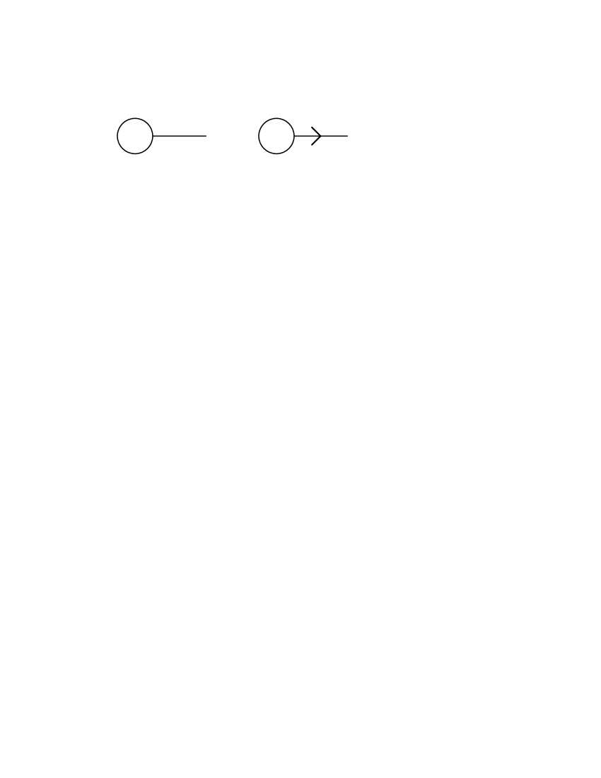
Figure 1: Diagrams corresponding to the two terms in the vertex operator $V_{1}$. The line represents the $\delta$ operator and the line with an arrow represents the $\delta^{\prime}$ operator.

Figure 2: Diagrams corresponding to the vertex operator $V_{2}$. Each additional line represents an additional $\delta$ operator.

The vertex operators can be represented diagramatically by vertices with external legs representing the $\delta$ operators (see figure 1 and figure 2). Each diagram contributes to the heat kernel (38), or equivalently to the zeta function via a Mellin transform,

$$\zeta_{k}(s)=\int d^{4}x{1\over\Gamma(s)}\int t^{s-1}Z(t)\langle...\rangle dt.$$ (44)

The one loop effective action is given by $W={\textstyle{1\over 2}}\zeta^{\prime}(0)$.

4 Second order calculation

We now perform the calculation of the contribution to the kinetic terms to second order. There are only three diagrams that contribute to the effective action. Other diagrams are zero due to the proper time integrals (see appendix A) or theta integrals (see appendix B).

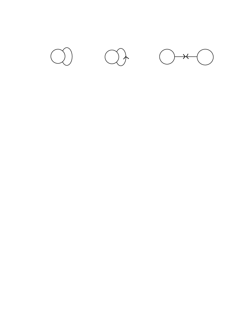
Figure 3: The non-zero diagrams: (a) gives a total divergence; (b) and (c) cancel out.

The first diagram is shown in figure 3a with one second order vertex and one contraction $D(t_{1},t_{1})$. This diagram gives a contribution to the heat kernel of (see equation (38)),

$$Z(t)\langle(3a)\rangle=-\frac{1}{2}\frac{1}{(4\pi t)^{2}}(\partial^{\mu}a_{\mu}-2a^{2})\frac{1}{3}t^{2}\sum_{n}e^{-\omega_{n}^{2}t}\omega_{n}^{2},$$ (45)

where the first factor is a symmetry factor and the first integral in (A7) has been used. The contribution of the diagram to the zeta function (denoted by $\zeta_{a}$) is given by equation (44),

$$\zeta_{a}(s)=-\frac{1}{16\pi^{2}}\int d^{4}x\frac{1}{6}(\partial^{\mu}a_{\mu}-2a^{2})\sum\omega_{n}^{2-2s}.$$ (46)

The sum can be expressed in terms of the Riemann zeta function and the derivative of the zeta function at $s=0$ is then

$$\zeta_{a}^{\prime}(0)=-\frac{1}{16\pi^{2}}{\pi^{2}\over 3}\zeta_{R}^{\prime}(-2)\int d^{4}x\,\beta^{-2}(\partial^{\mu}a_{\mu}-2a^{2}).$$ (47)

Using $a_{\mu}=\beta^{-1}\partial_{\mu}\beta$ and $\zeta_{R}^{\prime}(-2)=-\zeta_{R}(3)/(4\pi^{2})$, we get

$$\zeta_{a}^{\prime}(0)=-{1\over 16\pi^{2}}{1\over 48}\zeta_{R}(3)\pi^{2}\int d^{4}x(\partial^{2}\beta^{-2}),$$ (48)

This term is a total divergence and makes no contribution unless the 3-branes have a boundary.

The second term corresponds to the diagram in figure 3b. Here identities in appendix A and B have to be used. The diagram gives

$$Z(t)\langle(3b)\rangle={1\over(4\pi t)^{2}}\partial^{\mu}a_{\mu}\frac{1}{3}t^{2}\sum_{n}e^{-\omega_{n}^{2}t}\omega_{n}^{2}.$$ (49)

The contribution to the effective action is now

$$\zeta_{b}^{\prime}(0) = {1\over 16\pi^{2}}{2\pi^{2}\over 3}\zeta_{R}^{\prime}(-2)\int d^{4}x\,\beta^{-2}(\partial^{\mu}a_{\mu})$$ (50)

$$= {1\over 16\pi^{2}}{4\pi^{2}\over 3}\zeta_{R}^{\prime}(-2)\int d^{4}x\beta^{-4}(\partial\beta)^{2},$$

where we have used equation (26) and integrated by parts.

The third term corresponds to the diagram in figure 3c. For this diagram

$$Z(t)\langle(3c)\rangle=-\frac{1}{2}\frac{1}{(4\pi t)^{2}}a^{2}\frac{4}{3}t^{2}\sum_{n}e^{-\omega_{n}^{2}t}\omega_{n}^{2}.$$ (51)

The contribution to the effective action is

$$\zeta_{c}^{\prime}(0) = -\frac{1}{16\pi^{2}}{4\pi^{2}\over 3}\zeta_{R}^{\prime}(-2)\int d^{4}x\,\beta^{-2}a^{2}$$ (52)

$$= -\frac{1}{16\pi^{2}}{4\pi^{2}\over 3}\zeta_{R}^{\prime}(-2)\int d^{4}x\beta^{-4}(\partial\beta)^{2}.$$

Thus we see that equations (50) and (52) cancel. A similar calculation shows that the terms involving $b_{\mu}$ also cancel.

5 Conclusion

The method which we have used to evaluate the kinetic terms in the radion action for a brane world model can be extended quite easily. We have explicitly shown that there are no one loop second order corrections from massless fermions. It also follows by a simple extension of the arguments that there are no one loop second order corrections from any conformally invariant bulk fields on a conformally flat background or from massive fields on a flat background. The results are therefore not restricted to the Randall-Sundrum model and could be used for other brane world scenarios.

We might ask whether there are any derivative terms in the one loop corrections to the radion action. In fact, they do have to exist because of the renormalisation scale dependence. The renormalisation scale enters along with the $a_{5}$ heat kernel coefficient [23], which is of order $K^{4}$ in the extrinsic curvature and therefore eighth order in derivatives. We do not know yet whether this is the leading term in the derivative expansion.

Although the calculation of one loop effects may have a bearing on the hierarchy problem, the quantum corrections can also be considered in contexts which are independent of the hierarchy problem. For example, the cosmological evolution of these models appears to offer advantages over other stabalisation mechanisms in the way that the expansion couples to the energy density on the brane [22]. It would be interesting to persue this point in more detail.

Appendix A Propagators

There are three different propagators corresponding to the distinct combinations of the operators,

$$\langle T\delta^{\mu}(t_{1})\delta^{\nu}(t_{2})\rangle = \delta^{\mu\nu}D(t_{1},t_{2})$$ (53)

$$\langle T\delta^{\prime}_{\mu}(t_{1})\delta^{\nu}(t_{2})\rangle = \delta_{\mu}{}^{\nu}\overrightarrow{D}(t_{1},t_{2})$$ (54)

$$\langle T\delta^{\prime}_{\mu}(t_{1})\delta^{\prime}_{\nu}(t_{2})\rangle = \delta_{\mu\nu}\stackrel{{\scriptstyle\leftrightarrow}}{{D}}(t_{1},t_{2}).$$ (55)

These can be evaluated using the creation and annihilation operators defined in [14], leading to

$$D(t_{1},t_{2}) = 2\hbox{min}(t_{1},t_{2})-2t^{-1}t_{1}t_{2}$$ (56)

$$\overrightarrow{D}(t_{1},t_{2}) = 2\theta(t_{2}-t_{1})-2t^{-1}t_{2}$$ (57)

where $\theta(t)=1$ for $t\geq 0$ and zero otherwise. The third contraction evaluates to $-2t^{-1}$, but we replace (55) with

$$\stackrel{{\scriptstyle\leftrightarrow}}{{D}}(t_{1},t_{2})=2\delta(t_{1}-t_{2})-2t^{-1}$$ (58)

in order to reduce the number of vertices. The relevant time integrals of the propagators are:

$$\int_{0}^{t}D(t_{1},t_{1})dt_{1}=\frac{1}{3}t^{2} \int_{0}^{t}D(t_{1},t_{2})dt_{1}dt_{2}=\frac{1}{6}t^{3}$$

$$\int_{0}^{t}\overrightarrow{D}(t_{1},t_{2})dt_{1}dt_{2}=0 \int_{0}^{t}t_{1}\overrightarrow{D}(t_{1},t_{2})dt_{1}dt_{2}=0$$

$$\int_{0}^{t}(\overrightarrow{D}(t_{1},t_{1})+\overleftarrow{D}(t_{1},t_{1}))dt_{1}=0 \int_{0}^{t}t_{1}(\overrightarrow{D}(t_{1},t_{1})+\overleftarrow{D}(t_{1},t_{1}))dt_{1}=-\frac{1}{3}t^{2}$$

$$\int_{0}^{t}\stackrel{{\scriptstyle\leftrightarrow}}{{D}}(t_{1},t_{2})dt_{1}dt_{2}=0 \int_{0}^{t}(t_{1}+t_{2})\stackrel{{\scriptstyle\leftrightarrow}}{{D}}(t_{1},t_{2})dt_{1}dt_{2}=0$$

$$\int_{0}^{t}Max(t_{1},t_{2})\stackrel{{\scriptstyle\leftrightarrow}}{{D}}(t_{1},t_{2})dt_{1}dt_{2}=-\frac{1}{3}t^{2} \int_{0}^{t}t_{1}t_{2}\stackrel{{\scriptstyle\leftrightarrow}}{{D}}(t_{1},t_{2})dt_{1}dt_{2}=\frac{1}{6}t^{3}$$ (59)

Appendix B Theta integrals

The $\theta$ direction is special because the modes in this coordinate are discrete, $\langle\theta|n\rangle=\sqrt{2}\cos(n\theta)$ for Neumann boundary conditions and $\langle\theta|n\rangle=\sqrt{2}\sin(n\theta)$ for Dirichlet boundary conditions. We need a way to replace a $\theta$ sandwiched between $e^{\Delta_{0}t}$ terms inside the $|kn\rangle$ matrix elements. For this we use the Cambell-Baker-Hausdorff formula,

$$e^{\Delta_{0}t}\,\theta_{c}\,e^{-\Delta_{0}t}=\overline{\theta}(t).$$ (60)

where $\overline{\theta}(t)$ is an operator

$$\overline{\theta}(t)=\theta_{c}-2\pi^{2}\beta^{-2}t\partial_{\theta}$$ (61)

An important contraction identity we require for figure 3c is

$$\langle n|T\overline{\theta}(t_{1})\partial_{\theta}\overline{\theta}(t_{2})\partial_{\theta}|n\rangle=-{\textstyle{1\over 12}}\beta^{2}\omega_{n}^{2}+4\omega_{n}^{2}{\rm max}(t_{1},t_{2})\pm\omega_{n}^{2}(t_{1}+t_{2})+4\omega_{n}^{4}t_{1}t_{2}.$$ (62)

The results for other $\theta$ dependent terms in the matrix elements are given by

$$\langle n|n\rangle=1 \langle n|\partial_{\theta}|n\rangle=0$$

$$\langle n|\theta_{c}\partial_{\theta}|n\rangle=\pm{1\over 2} \langle n|\theta_{c}^{2}|n\rangle={\pi^{2}\over 12}$$

$$\langle n|(\theta_{c}\partial_{\theta})^{2}|n\rangle=-{\pi^{2}n^{2}\over 12} \langle n|\partial_{\theta}^{2}|n\rangle=-n^{2}.$$ (63)

The upper signs correspond to Neumann boundary conditions and the lower to Dirichlet boundary conditions.

References

• [1] I. Antoniadis, Phys. Lett. B246 (1990) 377; N. Arkani-Hamed, S. Dimopoulos, G. Dvali, Phys. Lett. B429 (1998) 263; I. Antoniadis, N. Arkani-Hamed, S. Dimopoulos, G. Dvali, Phys. Lett. B436 (1998) 257.
• [2] L. Randall and R. Sundrum, Phys. Rev. Lett.  83, 3370 (1999)
• [3] J. Garriga, O. Pujolas and T. Tanaka, hep-th/0004109.
• [4] W. D. Goldberger and I. Z. Rothstein, Phys. Lett. B491 (2000) 339.
• [5] D. J. Toms, Phys. Lett B484 149 (2000).
• [6] A. Flachi and D. J. Toms, hep-th/0103077.
• [7] A. Flachi, I. G. Moss and D. J. Toms, ‘Quantized bulk fermions in the Randall-Sundrum brane model’, hep-th/0103138; A. Flachi, I. G. Moss and D. J. Toms, hep-th/0106076.
• [8] I. Brevik, K. A. Milton, S. Nojori and S. D. Odintsov, Nucl. Phys. B599 (2001) 305
• [9] E. Ponton, E. Poppitz, hep-ph/0105021.
• [10] W. D. Goldberger and M. B. Wise, Phys. Rev. Lett.  83, 4922 (1999)
• [11] D. J. Toms, in An Introduction to Kaluza-Klein Theories, edited by H. C. Lee (World Scientific, Singapore, 1984).
• [12] Modern Kaluza-Klein Theories, edited by T. Appelquist, A. Chodos, P.G.O. Freund (Addison-Wesley, 1987).
• [13] P. Candelas and S. Weinberg, Nucl. Phys. B237 397 (1984).
• [14] I. G. Moss and Wade Naylor Class. Quant. Grav. 16, 2611 (1999).
• [15] I. G. Moss and S. Poletti, Phys. Rev. D47 5477 (1993).
• [16] A. O. Barvinski, T. A. Osborn and Yu. V. Gusev J. Math Phys. 36 30 (1995).
• [17] G. A. Vilkoviski, in Quantum Theory of Gravity, ed S M Christensen (Adam Hilger, Bristol 1984)
• [18] Barvinski and G. A. Vilkoviski Nucl. Phys. B (1987). 282 163; A. O. Barvinski and G. A. Vilkoviski Nucl. Phys. B 333 471 (1990).
• [19] I. G. Avrimidi, Nucl. Phys. B 355 712 (1991); I. G. Avrimidi, Nucl. Phys. B 509 577 (1998) (erratum)
• [20] J. Khoury, B. A. Ovrut, P. J. Steinhardt and N. Turok, hep-th/0103239.
• [21] H. A. Chamblin and H. S. Reall, Nucl. Phys. B562 133 (1999)
• [22] A. Mennim and R. A. Battye, Class. Quantum Grav. 18 2171 (2001)
• [23] T. P. Branson, P. B. Gilkey, K. Kirsten and D. V. Vassilevich, Nucl. Phys. B563 603 (1999)