Dilatonic monopoles and ”hairy” black holes

Abstract

We study gravitating monopoles and non-abelian black holes of SU(2) Einstein-Yang-Mills-Higgs theory coupled to a massless dilaton. The domain of existence of these solutions is bounded and decreases with increasing dilaton coupling strength. The critical solutions of this system are Einstein-Maxwell-dilaton solutions.

1 Introduction

In SU(2) Einstein-Yang-Mills-Higgs (EYMH) theory, with the Higgs field in the adjoint representation, globally regular gravitating magnetic monopole solutions [1, 2, 3] emerge smoothly from the flat space ’t Hooft-Polyakov monopole [4], when gravity is coupled. Since the mass of the non-abelian monopole in flat space is proportional to the Higgs vaccum expectation value $v$, while the size of the monopole core is inversely proportional to $v$, the monopole size should become comparable to the Schwarzschild radius, when $v$ becomes sufficiently large, and the non-abelian monopole should implode to a black hole [5]. Thus regular magnetic monopoles should exist only in a limited domain of the EYMH parameter space.

Indeed, as revealed by numerical analysis [1, 2, 3], regular gravitating monopoles exist only up to a maximal value $\alpha_{\rm max}$ of the coupling constant $\alpha$ (which is proportional the Higgs vacuum expectation value $v$ and the inverse Planck mass). Beyond $\alpha_{\rm max}$ the only solutions with unit magnetic charge are embedded abelian solutions, namely Reissner-Nordstrøm (RN) black hole solutions. Thus $\alpha_{\rm max}$ limits the domain of the EYMH parameter space, where non-abelian monopole solutions exist.

Besides the maximal value of $\alpha$, $\alpha_{\rm max}$, the critical value of $\alpha$, $\alpha_{\rm cr}$, is of particular importance. As $\alpha$ approaches the critical value $\alpha_{\rm cr}\leq\alpha_{\rm max}$ [6], the non-abelian monopole solutions approach a critical solution with a degenerate horizon. Outside the horizon the critical solution corresponds to an extremal RN solution with unit charge, while it is non-singular inside the horizon. Thus at $\alpha_{\rm cr}$, the non-abelian monopole branch bifurcates with the branch of extremal RN black holes [1, 2, 3].

Distinct from embedded RN black holes, genuine non-abelian magnetically charged black hole solutions emerge from the globally regular magnetic monopole solutions, when a finite regular event horizon is imposed [1, 2, 7]. Representing counterexamples to the “no-hair” conjecture for black holes, these black hole solutions may be viewed as “black holes within monopoles” [1], and have been interpreted as bound monopole-black hole systems [8].

The domain of existence in parameter space of genuine non-abelian black hole solutions is also bounded [1, 2]. In particular, for a fixed value of the coupling constant $\alpha$ ($\alpha<\alpha_{\rm max}$), the domain of existence of non-abelian black hole solutions is bounded by a maximal value of the horizon radius $x_{h,\rm max}$ (which depends on $\alpha$), and only relatively small non-abelian black hole solutions exist, as predicted on general grounds [9].

Here we investigate the influence of a massless dilaton on the gravitating non-abelian monopole solutions, since dilatons appear naturally in many unified theories, including string theory. The influence of a massless dilaton on the non-abelian monopole solutions in flat space has remarkable similarities to the influence of gravity on the monopole solutions [10]. In particular, in flat space the non-abelian dilatonic monopole solutions exist only below a maximal value of the coupling constant $\gamma$ (which is proportional the Higgs vacuum expectation value $v$ and the dilaton coupling constant). As $\gamma$ approaches a critical value, the non-abelian dilatonic monopole solutions approach a critical solution, which corresponds to an embedded abelian dilatonic monopole solution. Thus the branch of regular non-abelian monopole solututions bifurcates with the branch of singular abelian monopole solutions [10].

Considering the influence of both gravity and a dilaton, we expect that the domain of existence in parameter space of the non-abelian monopoles in Einstein-Yang-Mills-Higgs-dilaton (EYMHD) theory should also be bounded. This expectation is in distinction to arguments from string theory, which suggest, that regular non-abelian dilatonic monopole solutions exist for any value of the coupling constant [11]. We furthermore expect that the non-abelian dilatonic monopole solutions should also show a critical behaviour, when the respective coupling constants are varied. In particular, the branch of gravitating non-abelian dilatonic monopoles should bifurcate with the corresponding branch of embedded abelian solutions, namely Einstein-Maxwell-dilaton (EMD) solutions [12].

We also investigate the influence of a dilaton on the non-abelian black hole solutions, and we determine their domain of existence in parameter space. Furthermore, we obtain simple relations between the dilaton field and the metric, and the dilaton charge and the mass for the monopoles and black holes [13].

We review the EYMHD action in section II, where we discuss the spherically symmetric ansatz, the field equations, the boundary conditions and the relations between metric and dilaton field. We discuss our numerical results for the globally regular monopole solutions in section III and for the non-abelian black hole solutions in section IV. The conclusions are presented in section V. We briefly review the numerical procedure in Appendix A.

2 SU(2) Einstein-Yang-Mills-Higgs-Dilaton Equations of Motion

2.1 SU(2) Einstein-Yang-Mills-Higgs-dilaton action

We consider the action of the EYMHD theory

$$S=S_{G}+S_{M}=\int L_{G}\sqrt{-g}d^{4}x+\int L_{M}\sqrt{-g}d^{4}x\ .$$ (1)

The gravity Lagrangian $L_{G}$ is given by

$$4\pi L_{G}=\frac{1}{4G}R\ ,$$ (2)

where $G$ is Newton‘s constant. The matter Lagrangian is given in terms of the gauge fields ${A_{\mu}}^{a}$, the Higgs fields ${\Phi}^{a}$, and the dilaton field $\Psi$ ($a=1,2,3$)

$$4\pi L_{M}=-\frac{1}{4}e^{2\kappa\Psi}F_{\mu\nu}^{a}F^{\mu\nu,a}-\frac{1}{2}\partial_{\mu}\Psi\partial^{\mu}\Psi-\frac{1}{2}D_{\mu}\Phi^{a}D^{\mu}\Phi^{a}-e^{-2\kappa\Psi}V(\Phi^{a})\ ,$$ (3)

with Higgs potential

$$V(\Phi^{a})=\frac{\lambda}{4}(\Phi^{a}\Phi^{a}-v^{2})^{2}\ ,$$ (4)

The non-abelian field strength tensor is given by

$$F_{\mu\nu}^{a}=\partial_{\mu}A_{\nu}^{a}-\partial_{\nu}A_{\mu}^{a}+g\varepsilon_{abc}A_{\mu}^{b}A_{\nu}^{c}\ ,$$ (5)

and the covariant derivative of the Higgs field in the adjoint representation by

$$D_{\mu}\Phi^{a}=\partial_{\mu}\Phi^{a}+g\varepsilon_{abc}A_{\mu}^{b}\Phi^{c}\ ,$$ (6)

$g$ denotes the gauge field coupling constant, $\kappa$ the dilaton coupling constant, $\lambda$ the Higgs field coupling constant, and $v$ the vacuum expectation value of the Higgs field.

2.2 Spherically symmetric ansatz

To construct static spherically symmetric dilatonic monopoles and black holes, we employ for the metric the static spherically symmetric Ansatz with Schwarzschild-like coordinates

$$ds^{2}=-A^{2}(r)N(r)dt^{2}+N^{-1}(r)dr^{2}+r^{2}d\theta^{2}+r^{2}\sin^{2}\theta d^{2}\varphi\ ,$$ (7)

with the metric functions $A(r)$ and

$$N(r)=1-\frac{2m(r)}{r}\ ,$$ (8)

where the metric function $m(r)$ is the mass function. For the gauge and Higgs fields, we use the purely magnetic hedgehog ansatz [4, 1, 2]

$${A_{r}}^{a}={A_{t}}^{a}=0\ ,$$ (9)

$${A_{\theta}}^{a}=-\frac{1-K(r)}{g}{e_{\varphi}}^{a}\ ,\ \ \ \ {A_{\varphi}}^{a}=\frac{1-K(r)}{g}\sin\theta{e_{\theta}}^{a}\ ,$$ (10)

$${\Phi}^{a}=vH(r){e_{r}}^{a}\ .$$ (11)

A non-vanishing time-component of the gauge field would lead to dyon solutions [14, 15].

The dilaton is a scalar field depending only on $r$

$$\Psi=\Psi(r)\ .$$ (12)

2.3 Field equations

Let us now introduce dimensionless coordinates and fields

$$x=rgv\ ,\ \ \mu=mgv\ ,\ \ \phi=\frac{\Phi}{v}\ ,\ \ \psi=\frac{\Psi}{v}\ .$$ (13)

The Lagrangian and the resulting set of differential equations then depend only on three dimensionless couplings constants, $\alpha$, $\beta$ and $\gamma$,

$$\alpha=\sqrt{G}v=\frac{M_{W}}{gM_{\rm Pl}}\ ,\ \ \beta=\frac{\sqrt{\lambda}}{g}=\frac{M_{H}}{\sqrt{2}M_{W}}\ ,\ \ \gamma=\kappa v=\frac{\kappa M_{W}}{g}\ ,$$ (14)

where $M_{W}=gv$, $M_{H}=\sqrt{2\lambda}v$ and $M_{\rm Pl}=1/\sqrt{G}$. Special cases are $\kappa=\sqrt{G}$ (i.e. $\gamma=\alpha$), corresponding to string theory, and $\kappa^{2}=G\frac{(2+n)}{n}$ (i.e. $\gamma=\sqrt{\frac{2+n}{n}}\alpha$), corresponding to $(4+n)$-dimensional Kaluza-Klein theory [12].

Inserting the Ansatz into the Lagrangian and varying with respect to the matter fields yields the Euler-Lagrange equations

$$(e^{2\gamma\psi}ANK^{\prime})^{\prime}=A(e^{2\gamma\psi}\frac{K(K^{2}-1)}{x^{2}}+H^{2}K)\ ,$$ (15)

$$(x^{2}ANH^{\prime})^{\prime}=AH(2K^{2}+\beta^{2}x^{2}e^{-2\gamma\psi}(H^{2}-1))\ ,$$ (16)

$$(x^{2}AN\psi^{\prime})^{\prime}=2\gamma A(e^{2\gamma\psi}(N(K^{\prime})^{2}+\frac{(K^{2}-1)^{2}}{2x^{2}})-e^{-2\gamma\psi}\frac{\beta^{2}x^{2}}{4}(H^{2}-1)^{2})\ ,$$ (17)

where the prime denotes the derivative with respect to $x$.
Variation with respect to the metric yields the Einstein equations

$$G_{\mu\nu}=2\alpha^{2}T_{\mu\nu}\ ,$$ (18)

where $T_{\mu\nu}$ is the energy-momentum tensor

$$4\pi T_{\mu\nu}=g_{\mu\nu}L_{M}-2\frac{\partial L_{M}}{\partial g^{\mu\nu}}\ .$$ (19)

With the following combinations of the Einstein equations

$$G_{tt}=2\alpha^{2}T_{tt}=-2\alpha^{2}A^{2}NL_{M}\ ,$$ (20)

$$g^{rr}G_{rr}-g^{tt}G_{tt}=-4\alpha^{2}N\frac{\partial L_{M}}{\partial N}\ ,$$ (21)

we obtain for the metric functions $\mu$ and $A$ the differential equations

$$\mu^{\prime}=\alpha^{2}\left(e^{2\gamma\psi}N(K^{\prime})^{2}+\frac{1}{2}Nx^{2}(H^{\prime})^{2}+\frac{1}{2x^{2}}(K^{2}-1)^{2}e^{2\gamma\psi}+K^{2}H^{2}\right.\\$$

$$+\left.\frac{\beta^{2}}{4}x^{2}(H^{2}-1)^{2}e^{-2\gamma\psi}+\frac{1}{2}Nx^{2}(\psi^{\prime})^{2}\right)\ ,$$ (22)

$$A^{\prime}=\alpha^{2}xA\left(\frac{2(K^{\prime})^{2}}{x^{2}}e^{2\gamma\psi}+(H^{\prime})^{2}+(\psi^{\prime})^{2}\right)\ .$$ (23)

For $\gamma\equiv 0$, the dilaton decouples, $\psi\equiv 0$, and the set of equations reduces to the EYMH equations studied previously [1, 2, 3].

2.4 Boundary conditions

For the system of three second order equations, Eqs. (15)-(17), and two first order equations, Eqs. (22)-(23), we need to specify eight boundary conditions.

2.4.1 Dilatonic monopoles

Let us first consider the boundary conditions for static globally regular solutions with finite energy, which are asymptotically flat. Regularity at the origin requires the boundary conditions

$$K(0)=1\ ,\ \ H(0)=0\ ,\ \ \partial_{x}\psi|_{x=0}=0\ ,\ \ \mu(0)=0\ .$$ (24)

At infinity asymptotic flatness and finite energy impose the boundary conditions

$$K(\infty)=0\ ,\ \ H(\infty)=1\ ,\ \ \psi(\infty)=0\ ,\ \ A(\infty)=1\ ,$$ (25)

where the condition on $\psi$ can be imposed because of dilatational symmetry [16], and the condition on $A$ fixes the time coordinate. Note, that the value of the metric function $\mu$ at infinity determines the dimensionless mass of the solutions, $\mu(\infty)/\alpha^{2}$.

2.4.2 Dilatonic black holes

To construct black hole solutions which possess a regular event horizon at radius $x_{h}$, corresponding boundary conditions must be imposed at the horizon. Regularity at the horizon requires for the matter functions

$$N^{\prime}K^{\prime}=\frac{K(K^{2}-1)}{x^{2}}+e^{-2\gamma\psi}H^{2}K\ ,$$ (26)

$$N^{\prime}H^{\prime}=\frac{H}{x^{2}}(2K^{2}+\beta^{2}x^{2}e^{-2\gamma\psi}(H^{2}-1))\ ,$$ (27)

$$N^{\prime}\psi^{\prime}=\frac{2\gamma}{x^{2}}(e^{2\gamma\psi}(N(K^{\prime})^{2}+\frac{(K^{2}-1)^{2}}{2x^{2}})-e^{-2\gamma\psi}\frac{\beta^{2}x^{2}}{4}(H^{2}-1)^{2})\ ,$$ (28)

and for the metric functions

$$\mu(x_{h})=\frac{x_{h}}{2}\ ,$$ (29)

and $A(x_{h})<\infty$. At infinity, the black hole solutions satisfy the same boundary conditions as the globally regular solutions, Eqs. (25).

2.5 Relations between metric functions and dilaton field

In Einstein-Yang-Mills-dilaton (EYMD) theory, relations between the metric functions and dilaton field are known [13]. In the following we demonstrate, that corresponding relations hold in EYMHD theory.

Let us introduce the abbreviations

$$E_{A}=N(K^{\prime})^{2}+{(K^{2}-1)^{2}\over{2x^{2}}}\ ,\ \ E_{V}=\beta^{2}{x^{2}\over 4}(H^{2}-1)^{2}\ ,$$

$$E_{H}={1\over 2}Nx^{2}(H^{\prime})^{2}+K^{2}H^{2}\ ,\ \ F=e^{2\gamma\psi}\ .$$ (30)

In terms of these the dilaton equation and the first Einstein equation read,

$$(x^{2}AN\psi^{\prime})^{\prime}=2\gamma A(FE_{A}-F^{-1}E_{V})\ ,$$ (31)

$$\mu^{\prime}=\alpha^{2}(FE_{A}+E_{H}+F^{-1}E_{V}+{1\over 2}Nx^{2}(\psi^{\prime})^{2})\ .$$ (32)

Contraction of the Einstein equations yields for the curvature scalar $R$

$$-R=2\alpha^{2}\left(-N(\psi^{\prime})^{2}-{4\over{x^{2}}}F^{-1}E_{V}-{2\over{x^{2}}}E_{H}\right)\ .$$ (33)

Combination of these equations gives [13]

$$(x^{2}AN\psi^{\prime})^{\prime}=\frac{2\gamma A}{\alpha^{2}}({\mu^{\prime}}-{1\over 4}x^{2}R)\ .$$ (34)

With

$$Ax^{2}R=-\left[x^{2}(2A^{\prime}N+AN^{\prime})\right]^{\prime}+4A\mu^{\prime}\ ,$$ (35)

we obtain for the dilaton field the equation

$$(ANx^{2}\psi^{\prime})^{\prime}=\frac{\gamma}{2\alpha^{2}}\left(x^{2}(2A^{\prime}N+AN^{\prime})\right)^{\prime}\ .$$ (36)

This equation can be integrated, yielding

$$\psi^{\prime}=\frac{\gamma}{2\alpha^{2}}\left(\ln(A^{2}N)\right)^{\prime}+\frac{C}{ANx^{2}}\ ,$$ (37)

with integration constant $C$.

We can now derive the global relations between mass $\mu(\infty)/\alpha^{2}$ and dilaton charge $D$, defined via

$$\psi(x)\stackrel{{\scriptstyle x\rightarrow\infty}}{{\longrightarrow}}-\frac{D}{x}\ .$$ (38)

Considering first the regular solutions, we integrate Eq. (36) from zero to infinity, and take into account the asymptotic behaviour of the dilaton field, Eq. (38), and of the metric functions

$$A^{\prime}(x)\propto O(x^{-3}),\ \ N^{\prime}(x)\propto\frac{2\mu(\infty)}{x^{2}}+O(x^{-3})\ ,$$ (39)

as well as $N(\infty)=A(\infty)=1$. This yields the relation between the dilaton charge and the mass of the solution [13]

$$D=\gamma\frac{\mu(\infty)}{\alpha^{2}}\ .$$ (40)

Consequently the integration constant $C$ in Eq. (37) vanishes for regular solutions. Integrating Eq. (37) from $x$ to infinity then gives a simple relation between dilaton field and $tt$-component of the metric [13]

$$\psi(x)=\frac{\gamma}{2\alpha^{2}}\ln(A^{2}N)=\frac{\gamma}{2\alpha^{2}}\ln(-g_{tt})\ .$$ (41)

For black hole solutions we integrate Eq. (36) from the horizon to infinity. With the appropriate boundary conditions we thus obtain for black holes the relation [13]

$$D=\frac{\gamma}{\alpha^{2}}\left(\mu(\infty)-\frac{1}{2}x^{2}AN^{\prime}|_{x_{\rm H}}\right)\ .$$ (42)

The integration constant $C$ therefore does not vanish for black holes.

3 Dilatonic Monopoles

The non-abelian magnetic monopole solutions of Yang-Mills-Higgs (YMH) theory [4] persist in EYMH theory [1, 2, 3], when gravity is coupled, and in YMHD theory [10], when a dilaton field is coupled, for small values of the respective coupling constants. In both cases, the solutions bifurcate with an abelian solution at a critical value of the respective coupling constant.

Here we construct non-abelian magnetic monopoles, coupled to both gravity and a dilaton field. We solve the set of differential equations Eqs. (15)-(17) and Eqs. (22)-(23) numerically (see Appendix A for details), subject to the boundary conditions Eqs. (24)-(25). We show, that the gravitating dilatonic non-abelian magnetic monopole solutions also bifurcate with an abelian solution, an extremal EMD solution [12].

3.1 Monopoles in EYMH theory

Let us begin by briefly recalling the EYMH results for gravitating monopoles obtained in [1, 2, 3], corresponding to the limit $\gamma=0$ of EYMHD theory.

For a fixed value of the Higgs self-coupling $\beta$, a branch of gravitating non-abelian monopole solutions emerges smoothly from the flat space monopole solution, when $\alpha$ is increased. This branch exists on the interval $0\leq\alpha\leq\alpha_{\rm max}$. We refer to this branch as main branch. The maximal value of $\alpha$, $\alpha_{\rm max}$, decreases with increasing $\beta$.

For vanishing and small values of $\beta$, a short second branch of non-abelian monopole solutions is present on the interval $\alpha_{\rm cr}\leq\alpha\leq\alpha_{\rm max}$, and bifurcates with the main branch at $\alpha_{\rm max}$. We refer to this branch as secondary branch. At $\alpha_{\rm cr}$ the secondary branch bifurcates with a branch of embedded abelian solutions, the extremal RN solutions of Einstein-Maxwell (EM) theory, carrying unit magnetic charge and mass $\mu_{\rm RN}(\infty)/\alpha^{2}=1/\alpha$. For larger values of $\beta$, the secondary branch disappears, and $\alpha_{\rm cr}=\alpha_{\rm max}$ [1, 2]. Increasing $\beta$ further leads to a new phenomenon [3, 17].

Let us now consider, how the solutions approach the critical solution as $\alpha\rightarrow\alpha_{\rm cr}$, while $\beta$ is kept fixed. The metric function $N(x)$ possesses a minimum, which decreases monotonically as $\alpha\rightarrow\alpha_{\rm cr}$. At $\alpha_{\rm cr}$ the minimum of $N(x)$ reaches zero at the value of the radial coordinate $x=x_{h}=\alpha_{\rm cr}$. For $x\geq x_{h}$, the metric function $N(x)$ of the critical solution is identical to the metric function $N_{\rm RN}(x)=(1-\alpha_{\rm cr}/x)^{2}$ of the extremal RN solution, whereas it is different from the abelian function for $x\leq x_{h}$. $x_{h}$ represents the event horizon of the RN black hole.

Likewise, the matter field functions $K(x)$ and $H(x)$ approach the constant values $K_{\rm RN}(x)=0$ and $H_{\rm RN}(x)=1$ of the extremal RN solution as $\alpha\rightarrow\alpha_{\rm cr}$ for $x\geq x_{h}$, whereas they tend to non-trivial functions for $x\leq x_{h}$. Thus the critical solution reached at $\alpha_{\rm cr}$ is identical to an extremal RN solution outside the radius $x_{h}$, while it retains distinct non-abelian features inside the radius $x_{h}$.

3.2 Monopoles in YMHD theory

Let us now recall the YMHD results for dilatonic non-abelian monopoles in flat space [10], corresponding to the limit $\alpha=0$ of EYMHD theory. The dilatonic non-abelian monopoles in YMHD theory have many features in common with the non-abelian monopoles in curved space.

When the dilaton is coupled, the main branch of dilatonic non-abelian monopoles emerges smoothly from the ’t Hooft-Polyakov monopole, when $\gamma$ is increased, while the Higgs self-coupling $\beta$ is kept fixed. The main branch extends up to a maximal value of $\gamma$, $\gamma_{\rm max}$. For vanishing and small values of $\beta$, a secondary branch exists on the interval $\gamma_{\rm cr}\leq\gamma\leq\gamma_{\rm max}$, and bifurcates with the main branch at $\gamma_{\rm max}$. At $\gamma_{\rm cr}$ the secondary branch bifurcates with a branch of embedded abelian monopole solutions. For larger values of $\beta$, the secondary branch disappears, and $\gamma_{\rm cr}=\gamma_{\rm max}$ [10].

Intriguingly, even the numerical value for the maximal coupling constant $\gamma_{\rm max}$ is almost identical to the maximal coupling constant $\alpha_{\rm max}$ (for $\beta=0$).

3.3 Monopoles in EYMHD theory

Let us now consider how the presence of both gravity and a massless dilaton field affects the non-abelian monopoles. Generalizing the observations from EYMH and YMHD theory, we expect, that non-abelian monopoles in EYMHD theory also show a critical behaviour, when the respective coupling constants $\alpha$ and/or $\gamma$ are varied. In particular, the emerging branch of gravitating non-abelian dilatonic monopoles should bifurcate with the corresponding branch of embedded abelian solutions. Here these should be Einstein-Maxwell-dilaton (EMD) solutions [12]. Thus the domain of existence in parameter space of the gravitating dilatonic non-abelian monopoles should be bounded.

3.3.1 $\beta=0$

We first discuss the non-abelian monopoles of EYMHD theory for $\beta=0$.

Starting from the flat space dilatonic monopole solution for some value of the coupling constant $\gamma$, $\gamma\leq\gamma_{\rm cr}$ [10], we couple gravity by choosing a small but finite value of the coupling constant $\alpha$. Increasing $\alpha$, we obtain the main branch of dilatonic non-abelian monopole solutions, which exists on the interval $0\leq\alpha\leq\alpha_{\rm max}$. The short secondary branch of dilatonic non-abelian monopole solutions, present on the interval $\alpha_{\rm cr}\leq\alpha\leq\alpha_{\rm max}$, bifurcates with the main branch at $\alpha_{\rm max}$. At $\alpha_{\rm cr}$ the secondary branch bifurcates with a branch of embedded abelian solutions, which correspond to extremal EMD solutions, carrying unit magnetic charge and mass

$$\frac{\mu_{\rm EMD}(\infty)}{\alpha^{2}}=\frac{1}{\sqrt{\alpha^{2}+\gamma^{2}}}\ .$$ (43)

This is in complete accordance with our expectation [18].

Let us now consider in more detail how the non-abelian EYMHD monopole solutions approach the critical value of $\alpha$, when $\gamma$ is held fixed (and $\beta=0$). As in the EYMH system, the metric function $N(x)$ of the EYMHD system develops a minimum that decreases monotonically along the main and secondary branch. However, along the secondary branch the area close to the minimum starts to form a plateau, which broadens as $\alpha\rightarrow\alpha_{\rm cr}$. At the same time the function $N(x)$ becomes increasingly steep close to the origin. In the limit $\alpha\rightarrow\alpha_{\rm cr}$, the plateau extends up to $x=0$, and the non-abelian function $N(x)$ converges to the function $N_{\rm EMD}(x)$ of the extremal EMD solution with unit magnetic charge [12], and with the same values of $\alpha$ and $\gamma$. But since the value of the extremal EMD solution at the origin is given by [12],

$$N_{\rm EMD}(0)=\left(\frac{\gamma^{2}}{\alpha^{2}+\gamma^{2}}\right)\ ,$$ (44)

while the boundary conditions for the non-abelian solution require $N(0)=1$, convergence is pointwise. In contrast to the EYMH case, the minimum of the function $N(x)$ thus does not reach zero in the limit $\alpha\rightarrow\alpha_{\rm cr}$, when a dilaton field is present, so no horizon forms.

We illustrate the dependence of the metric function $N(x)$ of the EYMHD monopoles on the coupling strength $\alpha$ for $\gamma=0.5$ in Fig. 1a. The metric function $N(x)$ is shown for the maximal value of $\alpha$, $\alpha_{\rm max}=1.30702$, and for $\alpha=1.29459$, a value very close to the critical value $\alpha_{\rm cr}$, where a pronounced plateau is already visible. For comparison, the extremal EMD solution for $\alpha=1.29459$ is also shown.

The matter functions $K(x)$ and $H(x)$ also converge to their constant EMD values, $K_{\rm EMD}(x)=0$ and $H_{\rm EMD}(x)=1$, in the limit $\alpha\rightarrow\alpha_{\rm cr}$, Because of their respective boundary conditions at the origin, $K(0)=1$ and $H(0)=0$, convergence to the EMD solution is again pointwise.

Likewise, the dilaton function $\psi(x)$ approaches the EMD dilaton function

$$\psi_{\rm EMD}(x)=\frac{\gamma}{\alpha^{2}+\gamma^{2}}\ln(1-\frac{X_{-}}{X})\ ,$$ (45)

with

$$x/\alpha=X(1-\frac{X_{-}}{X})^{\gamma^{2}/(\alpha^{2}+\gamma^{2})}\ ,\ \ X_{-}=\left(\frac{\alpha^{2}+\gamma^{2}}{\alpha^{2}}\right)^{\frac{1}{4}}\ .$$ (46)

Since $X=X_{-}$ corresponds to the origin $x=0$, $\psi_{\rm EMD}(x)$ tends logarithmically to minus infinity for $x\rightarrow 0$. We illustrate the dilaton function $\psi(x)$ for $\gamma=0.5$ in Fig. 1b for $\alpha_{\rm max}=1.30702$ and $\alpha=1.29459$, i. e. for the same parameter values as in Fig. 1a. Convergence of the non-abelian functions $\psi(x)$ to the abelian function $\psi_{\rm EMD}(x)$, also shown in Fig. 1b, is clearly seen. In particular, the value of the dilaton function at the origin, $\psi(0)$, diverges for $\alpha\rightarrow\alpha_{\rm cr}$, in accordance with Eqs. (45)-(46).

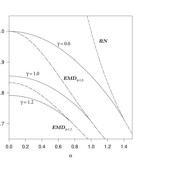
Figure 2: The dependence of the mass $\mu(\infty)/\alpha^{2}$ on $\alpha$ is shown for the non-abelian monopole solutions for three different values of $\gamma$, $\gamma=0$, $\gamma=1$ and $\gamma=1.2$. For comparison, the dependence of the mass on $\alpha$ is also shown for the corresponding abelian solutions (RN and EMD, respectively).

For a fixed value of $\gamma$, the mass $\mu(\infty)/\alpha^{2}$ of the non-abelian solutions decreases with increasing $\alpha$. In Fig. 2 we exhibit the dependence of the mass of the non-abelian monopoles on the coupling constant $\alpha$. In particular, we exhibit the mass of the EYMH solutions for $\gamma=0$ [2] and the mass of the EYMHD solutions for $\gamma=1.0$ and $1.2$. Also shown is the mass of the respective abelian solutions, namely the extremal RN solutions for $\gamma=0$ and the extremal EMD solutions for finite $\gamma$. The figure nicely illustrates the bifurcation of the non-abelian solutions with the corresponding abelian solutions. (The short secondary branches are very close to the abelian branches.)

Fig. 2 also shows, that for a fixed value of $\alpha$, the mass $\mu(\infty)/\alpha^{2}$ of the non-abelian solutions decreases with increasing $\gamma$. Interestingly, the mass of the critical solution, where the bifurcation takes place appears to be rather constant, as seen in Fig. 2. Given by Eq. (43), the mass of the critical solution depends only on the combination $\alpha^{2}+\gamma^{2}$. Since $\alpha_{\rm max}$ depends on $\gamma$, we conclude, that

$$\left(\alpha_{\rm max}(\gamma)\right)^{2}+\gamma^{2}\approx\rm const\ .$$ (47)

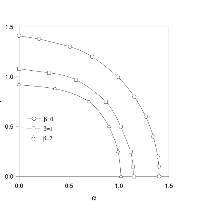
Figure 3: The domain of existence of the non-abelian monopole solutions in the $\alpha$-$\gamma$-plane is shown for three values of the Higgs self-coupling, $\beta=0$, $\beta=1$ and $\beta=2$.

As demonstrated in Fig. 3, the values $\alpha_{\rm max}(\gamma)$ lie indeed approximately on a circle, $\sqrt{\alpha_{\rm max}^{2}+\gamma^{2}}\approx 1.4$, which forms the boundary of the domain of existence of the non-abelian EYMHD monopole solutions.

When varying $\gamma$ while keeping $\alpha$ fixed, we obtain consistent results. In particular, for fixed $\alpha$, the main branch of dilatonic non-abelian monopole solutions exists on the interval $0\leq\gamma\leq\gamma_{\rm max}$, while the short secondary branch is present on the interval $\gamma_{\rm cr}\leq\gamma\leq\gamma_{\rm max}$. At $\gamma_{\rm cr}$ the secondary branch bifurcates with the corresponding branch of extremal EMD solutions [19].

Thus the dilaton field affects the gravitating non-abelian monopoles in a number of ways. Varying $\gamma$ along the main and secondary branch while keeping $\alpha$ fixed, the non-abelian core of the monopole solution shrinks and at the same time, the mass decreases. At the critical value of $\gamma$ the core shrinks to zero size, and the mass reaches the value of an extremal EMD solution, representing a naked singularity. This critical behaviour differs distinctly from the EYMH case, where the exterior part of the critical solution coincides with an abelian extremal black hole, and the interior part of the critical solution retains the non-abelian features.

One should keep in mind the scale invariance of EYMHD theory, though. The above discussion of the critical behaviour corresponds to the choice $\psi(\infty)=0$ for the value of the dilaton field at infinity, Eq. (25). This implies that the value of the dilaton field at the origin diverges for $\gamma\rightarrow\gamma_{\rm cr}$, $\psi(0)\rightarrow-\infty$. A rescaling of the solutions [16] such that $\psi(0)=0$ should yield a critical solution with a regular interior and a finite size monopole core, but with an asymptotically diverging dilaton field and a diverging mass [10, 20].

3.3.2 $\beta\neq 0$

We have performed a detailed analysis of the EYMHD monopole solutions for small values of $\beta$. Here the features observed for $\beta=0$ persist. The domain of existence shrinks with increasing $\beta$. But its boundary remains close to a circle for small values of $\beta$, becoming slightly deformed with increasing $\beta$. This is illustrated in Fig. 3 for $\beta=1$ and $\beta=2$.

While we have made an extensive analysis of the EYMHD monopole solutions for vanishing and small $\beta$, we have not been able to cover much of the parameter space for larger values of $\beta$. When trying to determine the domain of existence in the $\alpha$-$\gamma$-plane for larger values of $\beta$, we have encountered numerical problems [21]. Here new phenomena appear [22], which make the numerical analysis extremely difficult. Certainly further investigation of the non-abelian EYMHD monopole solutions for large values of $\beta$ is called for, but employment of another numerical procedure might be necessary.

4 Dilatonic Black Holes

Non-abelian black holes in EYMHD theory have many features in common with non-abelian black holes in EYMH theory. In particular, they are limited in size and they tend to critical abelian solutions at critical values of the horizon radius.

The black hole solutions of EYMHD theory depend on four parameters, $\alpha$, $\beta$, $\gamma$ and the horizon radius $x_{h}$. Here we limit the discussion to $\beta=0$. We construct the black hole solutions, by solving the set of differential equations Eqs. (15)-(17) and Eqs. (22)-(23) numerically (see Appendix A for details), subject to the boundary conditions Eqs. (25)-(28), thus the black hole solutions are asymptotically flat and they possess a regular horizon.

4.1 Black holes in EYMH theory

Let us again briefly recall some properties of the non-abelian black holes in EYMH theory [1, 2, 7, 3]. For a fixed value of the coupling constant $\alpha$ ($\alpha<\alpha_{\rm max}$), black hole solutions emerge from the globally regular solution, when a finite horizon radius is imposed. They persist up to a maximal value of the horizon radius $x_{h,\rm max}$, depending on $\alpha$. Thus the domain of existence of genuine non-abelian black hole solutions is bounded, and only relatively small non-abelian black hole solutions exist [9].

We dinstiguish two regions of black holes solutions with different critical behaviour. For a fixed value of $\alpha>\sqrt{3}/2$, the critical solution approached corresponds to an extremal RN solution. In contrast, for a fixed value of $\alpha<\sqrt{3}/2$, the critical solution approached corresponds to a non-extremal RN solution. In particular, for values of $\alpha$ not too close to $\alpha=\sqrt{3}/2$, two branches of solutions appear, a main branch $0\leq x_{h}\leq x_{h,\rm max}$ and a secondary branch $x_{h,\rm cr}\leq x_{h}\leq x_{h,\rm max}$.

4.2 Black holes in EYMHD theory

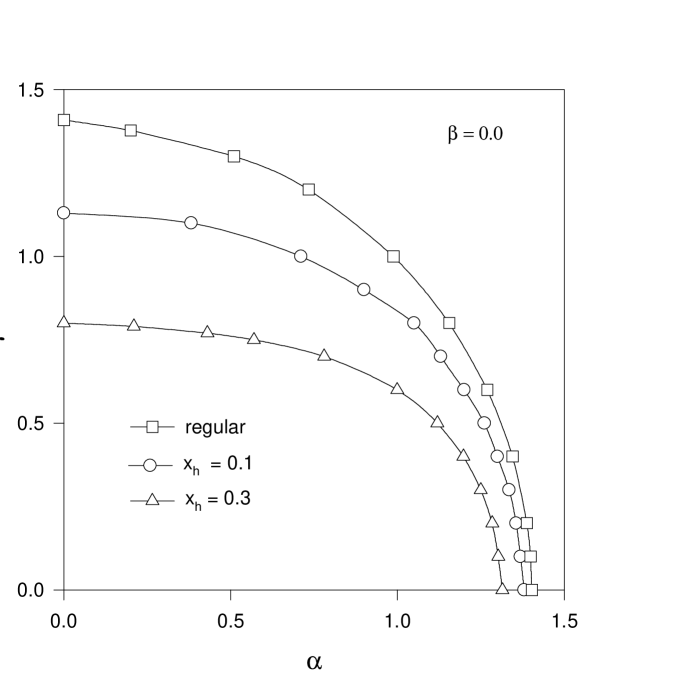
Figure 4: The domain of existence of the non-abelian black hole solutions in the $\alpha$-$\gamma$-plane is shown for $x_{h}=0.1$ and $x_{h}=0.3$. Also shown is the domain of existence of the non-abelian monopole solutions.

Let us first consider the domain of existence of the non-abelian black hole solutions. We recall, that the domain of existence of the non-abelian EYMHD monopole solutions is approximately bounded by a circle in the $\alpha$-$\gamma$-plane. Imposing a small but fixed horizon radius $x_{h}$, the domain of existence of the non-abelian EYMHD black hole solutions decreases with respect to the domain of existence of the regular solutions. With increasing size of the horizon, the domain of existence of the black hole solutions decreases further. Since the maximal value of $\gamma$, $\gamma_{\rm max}(\alpha=0)$ decreases stronger with increasing $x_{h}$ than the maximal value of $\alpha$, $\alpha_{\rm max}(\gamma=0)$, the domain of existence of the non-abelian black hole solutions is no longer approximately bounded by a circle in the $\alpha$-$\gamma$-plane for finite values of $x_{h}$. This is demonstrated in Fig. 4, which shows the domain of existence in the $\alpha$-$\gamma$-plane for the non-abelian black hole solutions with horizon radii $x_{h}=0.1$ and $x_{h}=0.3$, in addition to the domain of existence of the non-abelian monopole solutions.

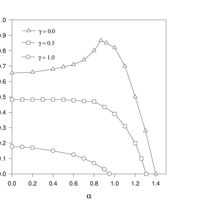
Figure 5: The domain of existence of the non-abelian black hole solutions in the $\alpha$-$x_{h}$-plane is shown for three values of the dilaton coupling constant, $\gamma=0$, $\gamma=0.5$ and $\gamma=1$.

In the $\alpha$-$x_{h}$-plane the domain of existence of the non-abelian black hole solutions decreases with increasing $\gamma$, as demonstrated in Fig. 5 for $\gamma=0$, $\gamma=0.5$ and $\gamma=1.0$ [23]. In the EYMH system, the domain of existence is separated into two distinct regions by the straight line $\alpha=x_{h}$, representing the extremal RN solutions. In particular, the maximum of the boundary curve $x_{h,\rm max}(\alpha)$ occurs on this line for $\alpha=\sqrt{3}/2$. As seen in Fig. 5, the boundary of the domain of existence in the $\alpha$-$x_{h}$-plane changes drastically with increasing $\gamma$. The boundary curve becomes rather smooth and the maximum disappears. We note, that in contrast to the EYMH case, in the EYMHD case abelian solutions exist for arbitrarily small values of the horizon radius $x_{h}$, since extremal EMD solutions have $x_{h}=0$.

While Fig. 5 demonstrates the dependence of the maximal value of $\alpha$, $\alpha_{\rm max}$, on $x_{h}$ for fixed $\gamma$, we now consider the dependence of the critical value of $\alpha$, $\alpha_{\rm cr}$, on $x_{h}$ for fixed $\gamma$. In the following we restrict the discussion to $\gamma=0.5$.

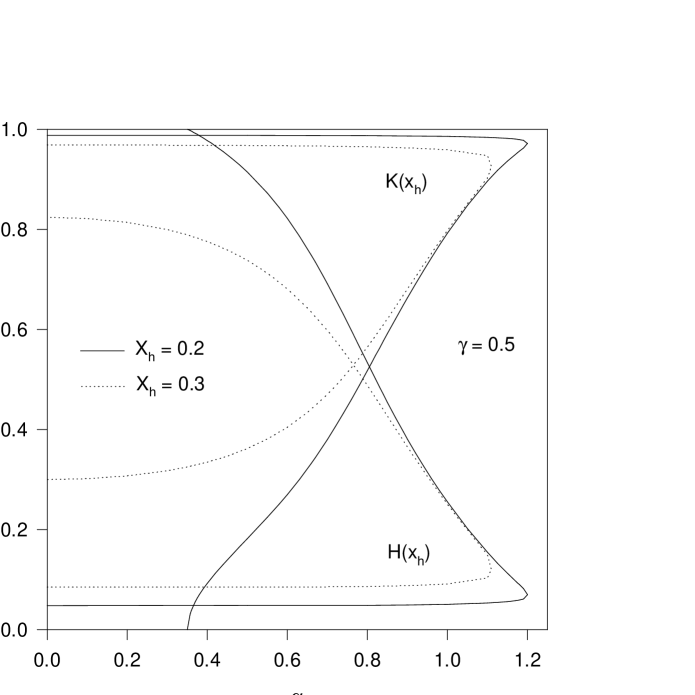
Figure 6: The values of the matter functions at the horizon, $K(x_{h})$ and $H(x_{h})$, of the non-abelian black hole solutions are shown for $\gamma=0.5$ and for $x_{h}=0.2$ and $x_{h}=0.3$.

For fixed $x_{h}$ and increasing $\alpha$, the main branch of solutions extends from $\alpha=0$ to $\alpha_{\rm max}(x_{h})$. At $\alpha_{\rm max}(x_{h})$ the main branch bifurcates with the secondary branch. Depending on the value of $x_{h}$, we observe two qualitatively different types of behaviour for the secondary branch. When $0\leq x_{h}(\gamma=0.5)\leq 0.22$, the secondary branch ends at a finite critical value of $\alpha$, whereas when $0.22\leq x_{h}(\gamma=0.5)\leq 0.48$, the secondary branch extends all the way to $\alpha=0$. This is demonstrated in Fig. 6, where the values of the matter functions at the horizon, $K(x_{h})$ and $H(x_{h})$, are shown for $x_{h}=0.2$ and $x_{h}=0.3$.

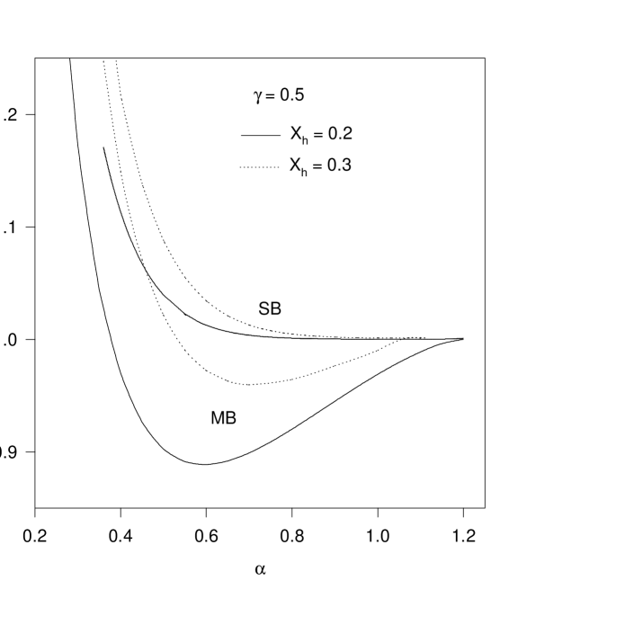
Figure 7: The mass ratio $\mu(\infty)/\mu_{\rm EMD}(\infty)$ of the non-abelian black hole solutions and the extremal EMD solutions is shown for $\gamma=0.5$ and for $x_{h}=0.2$ and $x_{h}=0.3$.

When decreasing $\alpha$ along the secondary branch for $0\leq x_{h}(\gamma=0.5)\leq 0.22$, it first appears, that the solution tends to an extremal EMD solution on the interval $x>x_{h}$ with a divergent derivative of the metric function $N$ at $x_{h}$. Indeed, the mass ratio $\mu(\infty)/\mu_{\rm EMD}(\infty)$, remains close to one on a large part of the secondary branch, as seen in Fig. 7. Decreasing $\alpha$ further, however, indicates that the critical solution is not an extremal EMD solution, but a non-extremal EMD solution. While for $\alpha\rightarrow\alpha_{\rm cr}$ the matter functions $K$ and $H$ approach their abelian values, $K(x_{h})\rightarrow 0$ and $H(x_{h})\rightarrow 1$, as seen in Fig. 6 for $x_{h}=0.2$, the mass ratio $\mu(\infty)/\mu_{\rm EMD}(\infty)$, tends to a value significantly greater than one, as seen in Fig. 7. The profiles of the metric function $N$ and the dilaton function $\psi$ support the conclusion as well, that the critical solution is a non-extremal EMD solution. In particular, the plateau of the metric function $N$, that forms when $\alpha$ is decreased from $\alpha_{\rm max}$, disappears again, when $\alpha$ is decreased further towards $\alpha_{\rm cr}$.

For $0.22\leq x_{h}(\gamma=0.5)\leq 0.48$ no critical value of $\alpha$ exists, instead the secondary branch extends all the way to $\alpha=0$, where $K(x_{h})$ and $H(x_{h})$ reach intermediate values in the interval $]0:1[$ in the limit $\alpha\rightarrow 0$, as demonstrated in Fig. 6 for $x_{h}=0.3$. The corresponding mass ratio $\mu(\infty)/\mu_{\rm EMD}(\infty)$ for $x_{h}=0.3$ is shown in Fig. 7.

5 Conclusions

We have constructed non-abelian monopoles and black holes in EYMHD theory, for vanishing and small Higgs self-coupling. Like the non-abelian monopole solutions of EYMH theory, the non-abelian monopole solutions of EYMHD theory reach critical solutions, when a critical value of the Higgs vacuum expectation value is reached. Therefore, the domain of existence of non-abelian monopole solutions is bounded also in EYMHD theory.

As the critical solution is approached, the branch of non-abelian EYMH monopole solutions bifurcates with a branch of embedded abelian solutions, corresponding to extremal RN solutions with unit charge. In the presence of a massless dilaton field, the branch of non-abelian EYMHD monopole solutions also bifurcates with a branch of embedded abelian solutions, which here correspond to extremal EMD solutions with unit charge. Thus without the dilaton field the critical solution is associated with a black hole solution, whereas in the presence of the dilaton field the critical solution is associated with a naked singularity.

Like the non-abelian black hole solutions of EYMH theory, the non-abelian black hole solutions of EYMHD theory are limited in size. Only relatively small black hole solutions exist [9]. The critical solutions reached at a critical value of the horizon radius $x_{h}$ also are associated with embedded abelian solutions, corresponding to RN black hole solutions in EYMH theory and to EMD black hole solutions in the presence of a dilaton field.

The boundary of the domain of existence of the non-abelian monopole solutions is approximately a circle in the $\alpha$-$\gamma$-plane. For non-abelian black hole solutions the domain of existence decreases with increasing horizon radius $x_{h}$ in the $\alpha$-$\gamma$-plane. In the $\alpha$-$x_{h}$-plane the domain of existence decreases with increasing $\gamma$, exhibiting a much smoother boundary line for finite values of $\gamma$ than for $\gamma=0$.

Besides presenting numerical results we have also derived an analytical formula relating the dilaton function and the metric in the case of the dilatonic monopoles, and we have given analytical relations between the mass and the dilaton charge for monopoles and black holes.

We have not yet considered the radial excitations of the dilatonic monopoles and black holes, which should be present, in analogy to the radial excitations of the EYMH solutions [1, 2].

EYMH theory also possesses static axially symmetric monopole and black hole solutions, which are not spherically symmetric [24]. These black hole solutions, in particular, show, that Israels theorem cannot be extended to EYMH theory [25]. Currently, we are investigating such static axially symmetric solutions also in EYMHD theory.

Acknowledgements: One of us (B.H.) acknowledges the Belgium F.N.R.S. for financial support.

6 Appendix A: Numerical Procedure

To construct the dilatonic monopole and black hole solutions numerically, we employ a collocation method for boundary-value ordinary differential equations developed by Ascher, Christiansen and Russell [26]. The set of non-linear coupled differential equations Eqs. (15) -(17) and Eqs. (22) -(23) is solved using the damped Newton method of quasi-linearization. At each iteration step a linearized problem is solved by using a spline collocation at Gaussian points. Since the Newton method works very well, when the initial approximate solution is close to the true solution, the dilatonic monopole and black hole solutions for varying parameters $\alpha$, $\beta$, $\gamma$ and $x_{h}$ are obtained by continuation.

The linearized problem is solved on a sequence of meshes until the required accuracy is reached. For a particular mesh $x_{i}=x_{1}<x_{2}<...<x_{N+1}=x_{o}$, where $x_{i}$ and $x_{o}$ are the boundaries of the interval, and $h_{i}=x_{i+1}-x_{i}$, $h={\rm max}_{1\leq i\leq N}h_{i}$, a collocation solution $\vec{v}$ $(x)=(v_{1},v_{2},...v_{d})$ is determined. Each component $v_{n}(x)\in C^{m_{n}-1}[x_{i},x_{o}]$, is a polynomial of degree smaller than $k+m_{n}$, where $m_{n}$ is the order of the $n$-th equation, and $k$ is an integer bigger than the highest order of any of the differential equations. The collocation solution is required to satisfy the set of differential equations at the $k$ Gauss-Legendre points in each subinterval as well as the set of boundary conditions.

When approximating the true solution $u_{n}(x)$ by the collocation solution $v_{n}(x)$, an error estimate in each subinterval $x\in[x_{i},x_{i+1})$ is obtained from the expression

$$||u_{n}^{(l)}(x)-v_{n}^{(l)}(x)||_{(i)}=c_{n,l}|u_{n}^{(k+m_{n})}(x_{i})|h_{i}^{k+m_{n}-l}+O(h^{k+m_{n}-l+1})$$

$$l=0,....,m_{n}-1\ ,\ \ \ n=1,...,d\ ,$$ (48)

where $c_{n,l}$ are known constants. Also, using Eq. (48) a redistribution of the mesh points is performed to roughly equidistribute the error. With this adaptive mesh selection procedure, the equations are solved on a sequence of meshes until the successful stopping criterion is reached, where the deviation of the collocation solution from the true solution is below a prescribed error tolerance [26].

For the numerical solutions, we typically specified the error tolerance in the range $10^{-4}-10^{-6}$. The number of mesh points used in these calculations was typically about $350$. We calculated the dilatonic monopole solutions on the finite interval $[0,x_{o}]$ and the black hole solutions on the finite interval $[x_{h},x_{o}]$, where $x_{h}$ represents the horizon of the black hole, with $x_{o}$ ranging from $10^{2}$ to $10^{4}$.

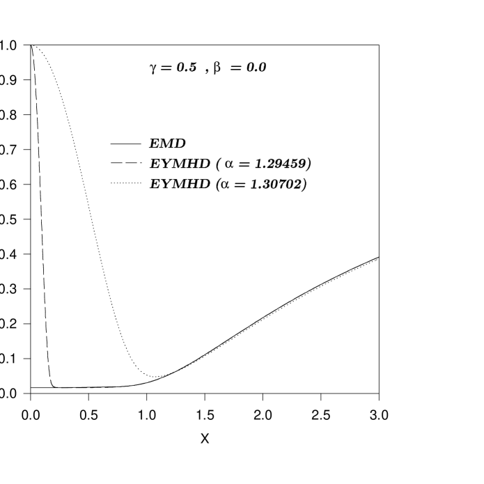
Figure 1a: The metric function $N(x)$ of the non-abelian monopole solutions is shown for $\gamma=0.5$ and two values of $\alpha$, the maximal value of $\alpha$, $\alpha_{\rm max}=1.30702$, and $\alpha=1.29459$, a value very close to the critical value $\alpha_{\rm cr}$. For comparison, the metric function $N_{\rm EMD}(x)$ of the extremal EMD solution for $\gamma=0.5$ and $\alpha=1.29459$ is also shown.

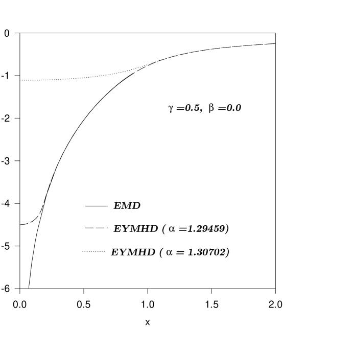
Figure 1b: Same as Fig. 1a for the dilaton function $\psi(x)$.

References

- [1] K. Lee, V.P. Nair and E.J. Weinberg, Phys. Rev. D45 (1992) 2751.
-
[2]
P. Breitenlohner, P. Forgacs and D. Maison,
Nucl. Phys. B383 (1992) 357;
P. Breitenlohner, P. Forgacs and D. Maison, Nucl. Phys. B442 (1995) 126. -
[3]
A. Lue and E.J. Weinberg,
Phys. Rev. D60 (1999) 084025;
Y. Brihaye, B. Hartmann, and J. Kunz, Phys. Rev. D62 (2000) 044008. -
[4]
G. ‘t Hooft,
Nucl. Phys. B79 (1974) 276;
A. M. Polyakov, JETP Lett. 20 (1974) 194. - [5] J. A. Frieman and C. T. Hill, SLAC-Report No. SLAC-PUB-4283, 1987 (unpublished).
- [6] For vanishing and small Higgs mass [2], while for large Higgs mass the Lue-Weinberg phenomenon occurs [3].
- [7] P. C. Aichelburg and P. Bizon, Phys. Rev. D48 (1993) 607.
- [8] A. Ashtekar, A. Corichi, and D. Sudarsky Class. Quant. Grav. 18 (2001) 919.
- [9] D. Nunez, H. Quevedo, and D. Sudarsky, Phys. Rev. Lett. 76 (1996) 571.
- [10] P. Forgacs and J. Gyueruesi, Phys. Lett. B366 (1996) 205.
-
[11]
J. A. Harvey and J. Liu,
Phys. Lett. B268 (1991) 40;
J. P. Gauntlett, J. A. Harvey and J. Liu, Nucl. Phys. B409 (1993) 363. -
[12]
G. W. Gibbons and K. Maeda,
Nucl. Phys. B298 (1988) 741;
D. Garfinkle, G. T. Horowitz and A. Strominger, Phys. Rev. D43 (1991) 3140. - [13] B. Kleihaus, J. Kunz and A. Sood, Phys. Rev. D54 (1996) 5070.
- [14] B. Julia and A. Zee, Phys. Rev. D11 (1975) 2227.
-
[15]
Y. Brihaye, B. Hartmann, J. Kunz,
Phys. Lett. B441 (1998) 77;
Y. Brihaye, B. Hartmann, J. Kunz, and Nadege Tell, Phys. Rev. D60 (1999) 104016. - [16] The equations of motion are invariant under a shift , together with a rescaling . Therefore solutions regular at infinity can always be chosen to satisfy .
- [17] For larger values of , the non-abelian monopole solutions do not bifurcate with a branch of abelian solutions at . Instead the critical solution is essentially non-abelian [3].
- [18] Similarly, Einstein-Yang-Mills-dilaton solutions tend to an Einstein-Maxwell-dilaton solution (in the limit of large node number) [13], while Einstein-Yang-Mills solutions tend to an Einstein-Maxwell (RN) solution.
- [19] For instance, for we find , which is very close to .
- [20] G. Lavrelashvili and D. Maison, Nucl. Phys. B410 (1993) 407.
- [21] For , the determination of becomes numerically unreliable for , for , the analysis becomes problematic already for .
- [22] With increasing , the dilaton function develops a minimum close to the origin, with strongly increasing curvature.
- [23] We expect, that for , the maximal value of for which regular solutions of YMHD theory exist, the domain of existence shrinks to zero size.
-
[24]
B. Hartmann, B. Kleihaus, and J. Kunz,
Phys. Rev. Lett. 86 (2001) 1422;
B. Hartmann, B. Kleihaus, and J. Kunz, Axially symmetric monopoles and black holes in Einstein-Yang-Mills-Higgs theory, hep-th/0108129. - [25] S. A. Ridgway and E. J. Weinberg, Phys. Rev. D52 (1995) 3440.
-
[26]
U. Ascher, J. Christiansen, R. D. Russell,
A collocation solver for mixed order systems of boundary value problems,
Mathematics of Computation 33 (1979) 659;
U. Ascher, J. Christiansen, R. D. Russell, Collocation software for boundary-value ODEs, ACM Transactions 7 (1981) 209.