OPE between the Energy-Momentum Tensor and the Wilson Loop in ${\cal N}=4$ Super-Yang-Mills theory

1 Introduction

Conformal field theory (CFT) is important in modern particle physics in various contexts. The most powerful tool in the 2-dimensional CFT is the operator product expansion (OPE). The OPE between the energy-momentum tensor and an operator extracts its conformal weight.

We find it interesting to consider a similar situation regarding the Wilson loop in a conformally invariant Yang-Mills theory. In this paper, we investigate the OPE between the energy-momentum tensor and the Wilson loop in ${\cal N}=4$, 4-dimensional Super-Yang-Mills (SYM) theory with the $U(N)$ gauge group employing dimensional analysis and the properties of the energy-momentum tensor. We find that the Wilson loop in ${\cal N}=4$ SYM theory does not possess an anomalous dimension and that only the deformation of the loop occurs under the conformal transformation.

Another interesting related topic is the AdS/CFT correspondence. [1] The AdS/CFT correspondence enables one to evaluate such physical quantities as the multi-point function [4] and the expectation value of the Wilson loop [2]^,[3] in the strong coupling region. There have been ambitious attempts to compute the expectation value of the Wilson loop in the strong coupling region by means of quantum field theory [6]^,[7] for a direct test of the AdS/CFT correspondence. In particular, Gross and Drukker [7] pointed out that the expectation value of a circular Wilson loop in ${\cal N}=4$, 4-dimensional SYM theory is determined by an anomaly in the conformal transformation that relates a circular loop to a straight line and computed the expectation value of the circular Wilson loop to all orders in the $\frac{1}{N}$ expansion. However, their analysis is based on the Feynman gauge, and the generalization to the general gauge is non-trivial. We attempt to understand the conformal anomaly through the OPE between the energy-momentum tensor and the closed Wilson loop, taking advantage of its gauge invariance.

This paper is organized as follows. Section 2 is devoted to the study of the OPE between $T_{\mu\nu}(z)$ and $W[C]$ in the $U(N)$ gauge theory by means of dimensional analysis and the properties of the energy-momentum tensor. Section 3 presents the computation for the $U(1)$ gauge theory as a simple example of the general form investigated in the previous section. Section 4 contains the concluding remarks and the outlook for our research. The appendices contain the proofs of the formulae we derive in full detail.

2 General form of the OPE in the ${\cal N}=4$ SYM theory

In this section, we develop the OPE between the Wilson loop and the energy momentum tensor in the $U(N)$ SYM theory. The bosonic part of the Lagrangian and the Wilson loop are as follows:

$${\cal L} = \frac{1}{2G^{2}}\left[\frac{1}{2}(F_{\mu\nu})^{2}+(D_{\mu}\phi_{i})^{2}+([\phi_{i},\phi_{j}])^{2}+\xi(\partial^{\mu}A_{\mu})^{2}\right],$$

$$F_{\mu\nu} = \partial_{\mu}A_{\nu}-\partial_{\nu}A_{\mu}-i[A_{\mu},A_{\nu}],$$ (2.1)

$$D_{\mu}\phi_{i} = \partial_{\mu}\phi_{i}-i[A_{\mu},\phi_{i}],$$ (2.2)

$$W[C] = \frac{1}{N}\textrm{Tr}P\exp\left[\oint_{C}du\left\{iA_{\mu}(y(u))\frac{dy^{\mu}(u)}{du}+\phi_{i}(y(u))\theta^{i}(u)\right\}\right].$$ (2.3)

Throughout this paper, we use the following indices: $\mu,\nu,\cdots=0,1,2,3$ and $i,j,\cdots=4,5,\cdots,9$. Our analysis is carried out in Euclidean space with the metric $g_{\mu\nu}=\delta_{\mu\nu}=diag(1,1,\cdots,1)$. The indices of the scalar fields are contracted by $\delta_{ij}$. $G$ denotes the coupling constant. $W[C]$ is the Wilson loop in ${\cal N}=4$, 4-dimensional SYM theory, whose derivation is given in detail in a paper of Drukker, Gross and Ooguri. [5] $y^{\mu}(u)$ represents the coordinates of the Wilson loop. The parameter of the Wilson loop $u$ is an arc length parameter, and it satisfies $|\frac{dy_{\mu}(u)}{du}|=1$. $\theta_{i}(u)$ is chosen such that $\theta_{i}(u)\theta^{i}(u)=1$.

$T_{\mu\nu}(z)$ denotes the energy-momentum tensor of ${\cal N}=4$, 4-dimensional SYM theory, defined by

$$T_{\mu\nu}(z)=\frac{2}{\sqrt{g}}\frac{\delta{\cal L}}{\delta g^{\mu\nu}}.$$ (2.4)

The following two fundamental properties of the energy-momentum tensor play a crucial role in our analysis.

• tracelessness: ${T^{\mu}}_{\mu}(z)=0$. This implies the scale invariance of the action.

• divergencelessness: $\partial^{\mu}T_{\mu\nu}(z)=0$. This implies the conservation of the energy and momentum.

Before entering the analysis, let us review the well-known OPE in the 2-dimensional CFT. In considering the conformal Ward identity, we perform a contour integral around the operator $A(w)$. Therefore, ${\cal O}(z-w)^{-1}$ is the order of the weakest singularity that contributes to the conformal Ward identity. The OPE is expressed by

$$T(z)A(w) =$$ (lower-dimensional operators) (2.5)

$$+ \frac{h}{(z-w)^{2}}A(w)+\frac{\partial A(w)}{z-w}+\cdots.$$

An example of the lower-dimensional operators is the term of the central charge $\frac{\frac{c}{2}}{(z-w)^{4}}$, with $A(w)$ being the energy-momentum tensor. The coefficients of $\frac{1}{z-w}$ and $\frac{1}{(z-w)^{2}}$ represent the translation and the conformal weight of the operator, respectively. An important special case is a primary field, on which the OPE reduces to

$$T(z)A(w)=\frac{h}{(z-w)^{2}}A(w)+\frac{\partial A(w)}{z-w}+\cdots.$$ (2.6)

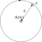
Fig. 1: The contour integral in the 2-dimensional CFT.

 

Let us next consider the OPE between $T_{\mu\nu}(z)$ and $W[C]$ in 4-dimensional Euclidean space. We perform the integral over the region wrapping the Wilson loop, and this is translated into an integral over the surface of the manifold. Let $y^{\mu}(u_{0})$ be the point on the Wilson loop nearest to the point $z^{\mu}$. In other words, we take the point $y^{\mu}(u_{0})$ so that the vector $z_{\mu}-y_{\mu}(u_{0})$ is perpendicular to the tangent vector of the Wilson loop $\frac{dy^{\mu}(u_{0})}{du}$:

$$(z_{\mu}-y_{\mu}(u_{0}))\frac{dy^{\mu}(u_{0})}{du}=0.$$ (2.7)

The dependence of the point $u_{0}$ on the coordinate $z_{\mu}$ is given by

$$\frac{\partial u_{0}}{\partial z^{\mu}}=\frac{\frac{dy_{\mu}(u_{0})}{du}}{1-(z_{\alpha}-y_{\alpha}(u_{0}))\frac{d^{2}y^{\alpha}(u_{0})}{du^{2}}}.$$ (2.8)

This can be derived by noting that the vector $(z_{\mu}+dz_{\mu})-y_{\mu}(u_{0}+du_{0})$ is also perpendicular to the tangent vector $\frac{dy_{\mu}(u_{0}+du_{0})}{du}$, where $du_{0}$ is the variation of the parameter $u_{0}$ accompanying an infinitesimal variation of the coordinate $dz_{\mu}$.

Let $S^{2}(u_{0})$ be the boundary of the 3-dimensional ball of a fixed radius $\epsilon$ that is perpendicular to the tangent vector $\frac{dy^{\mu}(u_{0})}{du}$ and has its center at $y_{\mu}(u_{0})$. We wrap the Wilson loop with the surface enveloping these spheres $S^{2}(u_{0})$, with $y^{\mu}(u_{0})$ running over the whole Wilson loop. We define the region inside this enveloping surface as ${\cal M}$. Its surface $\partial{\cal M}$ is, of course, the enveloping surface of the spheres $S^{2}(u_{0})$. Utilizing Gauss’s theorem, the conformal Ward identity for the Wilson loop is

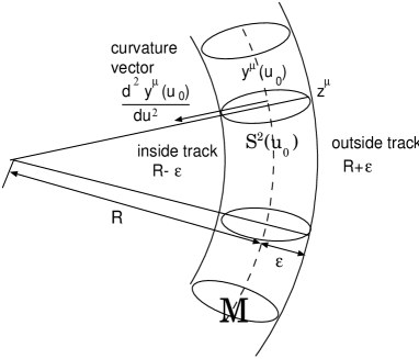
Fig. 3: We perform the integral over the surface enveloping the boundary of the 3-dimensional balls perpendicular to the Wilson loop.

$$\int_{\cal M}d^{4}z\partial^{\mu}[T_{\mu\nu}(z)W[C]v^{\nu}(z)]=\int du_{0}\int_{S^{2}(u_{0})}d\mathchar 28938\relax{\cal C}n^{\mu}T_{\mu\nu}(z)W[C]v^{\nu}(z).$$

(2.9)

The meanings of the quantities appearing in the above formula are as follows.

• The spacetime integral is performed over the manifold ${\cal M}$, in which the Wilson loop is included.

• $v^{\nu}(z)$ is a conformal Killing vector. Its explicit form is as follows:

  Translation: $$\hskip 8.53581ptv^{\nu}(z)=\xi^{\nu},$$ (2.10)

  Dilatation: $$\hskip 8.53581ptv^{\nu}(z)=\lambda z^{\nu},$$ (2.11)

  Special Conformal Transformation (SCT): $$\hskip 8.53581ptv^{\nu}(z)=2z^{\nu}(b_{\alpha}z^{\alpha})-b^{\nu}z^{2}.$$ (2.12)

• $d\mathchar 28938\relax$ denotes the spherical integral over $S^{2}(u_{0})$, and $n^{\mu}$ is the normal vector on the surface $\partial{\cal M}$.

• The measure ${\cal C}$ results from the difference between the inside track and the outside track. When the radius of curvature is $R$ and the radius of the sphere $S^{2}(u_{0})$ is $\epsilon$, the ratio of the length of the inside track and the outside track is $R-\epsilon:R+\epsilon$. Therefore, the measure must be a quantity corresponding to the value $1\mp\frac{\epsilon}{R}$. Now, the point $z_{\mu}$ resides on the sphere $S^{2}(u_{0})$, and the vector $z_{\mu}-y_{\mu}(u_{0})$ corresponds to $\epsilon$. The quantity corresponding to $\frac{1}{R}$ is the curvature vector $\frac{d^{2}y_{\mu}(u_{0})}{du^{2}}$ . Therefore, the measure is

  $${\cal C}=1-(z_{\alpha}-y_{\alpha}(u_{0}))\frac{d^{2}y^{\alpha}(u_{0})}{du^{2}}.$$ (2.13)

  The minus sign results from the fact that the vector $\frac{d^{2}y^{\alpha}(u_{0})}{du^{2}}$ is directed at the center of curvature.

Since we perform the integral over the sphere $S^{2}(u_{0})$ whose surface area is $4\pi\epsilon^{2}$, the weakest singularity in the OPE that contributes to the conformal Ward identity is ${\cal O}(z-y(u_{0}))^{-2}$.

We now investigate the OPE $T_{\mu\nu}(z)W[C]$. In the following analysis, we separate the OPE into three parts for convenience.

$$T_{\mu\nu}(z)W[C]=(T_{\mu\nu}(z)W[C])_{\textrm{c}}+(T_{\mu\nu}(z)W[C])_{\textrm{vec}}+(T_{\mu\nu}(z)W[C])_{\textrm{sca}}.$$ (2.14)

We hypothesize that the terms corresponding to the lower-dimensional operators do not emerge in the OPE $T_{\mu\nu}(z)W[C]$. In this equation, $(T_{\mu\nu}(z)W[C])_{\textrm{c}}$ denotes the terms containing $W[C]$ itself without any insertion of the fields into it, which corresponds to the term $\frac{h}{(z-w)^{2}}A(w)$ in the 2-dimensional CFT. The other two terms include the insertion of the fields $A_{\mu}(y(u_{0}))$ or $\phi_{i}(y(u_{0}))$ into $W[C]$. As we find later by means of dimensional analysis, the vector fields and the scalar fields are not inserted simultaneously, and we separate the terms into the contribution of the vector field and that of the scalar field. $(T_{\mu\nu}(z)W[C])_{\textrm{vec}}$ and $(T_{\mu\nu}(z)W[C])_{\textrm{sca}}$ denote the contributions with the insertion of the vector and the scalar fields, respectively.

$T(z)A(w)$	lower-dimensional operators	$\frac{h}{(z-w)^{2}}A(w)$	$\frac{\partial A(w)}{z-w}$
$T_{\mu\nu}(z)W[C]$	$-$	$(T_{\mu\nu}(z)W[C])_{\textrm{c}}$	$(T_{\mu\nu}(z)W[C])_{\textrm{vec}}$
			$(T_{\mu\nu}(z)W[C])_{\textrm{sca}}$

2.1 Contribution of $W[C]$ itself without field insertion

We first investigate the contribution of $W[C]$ itself $(T_{\mu\nu}(z)W[C])_{\textrm{c}}$. We express the OPE as a power series expansion in $z_{\mu}-y_{\mu}(u_{0})$, where $y_{\mu}(u_{0})$ is the nearest point on the Wilson loop to the point $z_{\mu}$. We first list the possible ingredients of this contribution:

$$\left(\frac{dy_{\mu}(u_{0})}{du}\right)^{A},\hskip 5.69054pt\left(\frac{d^{2}y_{\mu}(u_{0})}{du^{2}}\right)^{B},\hskip 5.69054pt\left(\frac{d^{3}y_{\mu}(u_{0})}{du^{3}}\right)^{C},\cdots$$

$$\left(z_{\mu}-y_{\mu}(u_{0})\right)^{D},\hskip 5.69054pt\left(\frac{1}{|z-y(u_{0})|}\right)^{E},\hskip 5.69054pt\left(\theta_{i}(u_{0})\frac{d^{2}\theta^{i}(u_{0})}{du^{2}}\right)^{F},\cdots.$$ (2.15)

Here we choose the theta parameter to satisfy $\theta_{i}(u_{0})\theta^{i}(u_{0})=1$, and it immediately follows that $\theta_{i}(u_{0})\frac{d\theta^{i}(u_{0})}{du}=\frac{1}{2}\frac{d}{du}(\theta_{i}(u_{0})\theta^{i}(u_{0}))=0$. The absolute value $|\frac{dy_{\mu}(u_{0})}{du}|$ is 1 by definition, and we have $\frac{dy_{\alpha}(u_{0})}{du}\frac{d^{2}y^{\alpha}(u_{0})}{du}=\frac{1}{2}\frac{d}{du}(\frac{dy^{\alpha}(u_{0})}{du}\frac{dy_{\alpha}(u_{0})}{du})=0$. These powers are restricted by the following conditions.

1. The singularity that contributes to the conformal Ward identity is at least ${\cal O}(z-y(u_{0}))^{-2}$. Therefore, $D-E\leq-2$.

2. The coefficient must have dimensions of $(\textrm{length})^{-4}$, and this gives the condition $-B-2C+D-E-2F=-4$.

3. We hypothesize that $z_{\mu}-y_{\mu}(u_{0})$, $\theta_{k}(u_{0})$, $\frac{dy_{\mu}(u_{0})}{du}$, $\frac{d^{2}y_{\mu}(u_{0})}{du^{2}}$ and $\frac{d^{3}y_{\mu}(u_{0})}{du^{3}}$ have non-negative powers. Hence $A$, $B$, $C$, $D$ and $F$ must each be 0 or a positive integer.

4. Since the coefficient must be a tensor of rank two, the total number of the indices must be even, so that $A+B+C+D$ is an even number.

5. The result should be invariant under the exchange $u\rightarrow-u$, so that $A+3C$ must be an even number.

The second and third conditions lead to the relation $D-E=-4+(B+2C+E+2F)\geq-4$. Since $B$, $C$, $E$ and $F$ are restricted to be 0 or positive integers, the possible singularity in the OPE is thus

$$D-E=-4,-3,-2.$$ (2.16)

For convenience we classify the contribution of $W[C]$ itself according to the order of the singularity:

$$(T_{\mu\nu}(z)W[C])_{\textrm{c}}=(T_{\mu\nu}(z)W[C])_{\textrm{c4}}+(T_{\mu\nu}(z)W[C])_{\textrm{c3}}+(T_{\mu\nu}(z)W[C])_{\textrm{c2}}.$$ (2.17)

Here $(T_{\mu\nu}(z)W[C])_{\textrm{c4}}$, $(T_{\mu\nu}(z)W[C])_{\textrm{c3}}$ and $(T_{\mu\nu}(z)W[C])_{\textrm{c2}}$ denote the contributions with the singularities of ${\cal O}(z-y(u_{0}))^{-4}$, ${\cal O}(z-y(u_{0}))^{-3}$, and ${\cal O}(z-y(u_{0}))^{-2}$ respectively.

2.1.1 Terms with singularities of ${\cal O}(z-y(u_{0}))^{-4}$

We first consider the terms with singularities of ${\cal O}(z-y(u_{0}))^{-4}$. Since $D-E=-4$, the powers of the other ingredients are

$$B=0,\hskip 5.69054ptC=0,\hskip 5.69054ptF=0,\hskip 5.69054ptA,D=\textrm{(even)}.$$ (2.18)

Thus, we find that the possible form of the OPE is

$$(T_{\mu\nu}(z)W[C])_{\textrm{c4}} = \frac{1}{24\pi^{2}|z-y(u_{0})|^{4}}\left[a_{1}g_{\mu\nu}+a_{2}\frac{dy_{\mu}(u_{0})}{du}\frac{dy_{\nu}(u_{0})}{du}\right.$$ (2.19)

$$\left.+a_{3}\frac{(z_{\mu}-y_{\mu}(u_{0}))(z_{\nu}-y_{\nu}(u_{0}))}{|z-y(u_{0})|^{2}}\right]W[C].$$

The coefficients $a_{1}$, $a_{2}$ and $a_{3}$ are determined by the tracelessness and divergencelessness conditions. The former condition is simple, and gives

$$4a_{1}+a_{2}+a_{3}=0.$$ (2.20)

The divergencelessness is less simple due to the dependence of the point $u_{0}$ on the coordinates, as computed in (2.8). The divergence is given by

$$\partial^{\mu}(T_{\mu\nu}(z)W[C])_{\textrm{c4}}=\frac{1}{24\pi^{2}}\left[-(4a_{1}+2a_{3})\frac{z_{\nu}-y_{\nu}(u_{0})}{|z-y(u_{0})|^{6}}\right.$$

$$\hskip 14.22636pt-\left.a_{3}\frac{(z_{\nu}-y_{\nu}(u_{0}))[(z_{\alpha}-y_{\alpha}(u_{0}))\frac{d^{2}y^{\alpha}(u)}{du^{2}}]}{|z-y(u_{0})|^{6}(1-(z_{\alpha}-y_{\alpha}(u_{0}))\frac{d^{2}y^{\alpha}(u_{0})}{du^{2}})}+a_{2}\frac{\frac{d^{2}y_{\nu}(u_{0})}{du^{2}}}{|z-y(u_{0})|^{4}}\right]W[C].$$

We require that only the strongest singularity of ${\cal O}(z-y(u_{0}))^{-5}$ vanish, because the weaker singularities may be canceled by the contribution of the terms in the OPE with weaker singularities. With this assumption, the divergencelessness gives the condition

$$4a_{1}+2a_{3}=0.$$ (2.21)

2.1.2 Terms with singularities of ${\cal O}(z-y(u_{0}))^{-3}$

These terms are evaluated in a similar fashion. Since we are now treating the terms of ${\cal O}(z-y(u_{0}))^{-3}$, the powers must satisfy $D-E=-3$, so that

$$B=1,\hskip 5.69054ptC=0,\hskip 5.69054ptF=0,\hskip 5.69054ptA=\textrm{(even)},\hskip 5.69054ptD=\textrm{(odd)}.$$ (2.22)

The possible form of the OPE is thus determined to be

$$(T_{\mu\nu}(z)W[C])_{\textrm{c3}} = \frac{1}{24\pi^{2}}\left[b_{1}\frac{(z_{\mu}-y_{\mu}(u_{0}))(z_{\nu}-y_{\nu}(u_{0}))(z_{\alpha}-y_{\alpha}(u_{0}))\frac{d^{2}y^{\alpha}(u_{0})}{du^{2}}}{|z-y(u_{0})|^{6}}\right.$$

$$+b_{2}\frac{(z_{\mu}-y_{\mu}(u_{0}))\frac{d^{2}y_{\nu}(u_{0})}{du^{2}}+(z_{\nu}-y_{\nu}(u_{0}))\frac{d^{2}y_{\mu}(u_{0})}{du^{2}}}{|z-y(u_{0})|^{4}}$$

$$+\left.b_{3}\frac{\frac{y_{\mu}(u_{0})}{du}\frac{y_{\nu}(u_{0})}{du}(z_{\alpha}-y_{\alpha}(u_{0}))\frac{d^{2}y^{\alpha}(u_{0})}{du^{2}}}{|z-y(u_{0})|^{4}}+b_{4}g_{\mu\nu}\frac{(z_{\alpha}-y_{\alpha}(u_{0}))\frac{d^{2}y^{\alpha}(u_{0})}{du^{2}}}{|z-y(u_{0})|^{4}}\right]W[C].$$

These coefficients are again determined by the tracelessness and divergencelessness condition. The former condition is trivial, and yields

$$b_{1}+2b_{2}+b_{3}+4b_{4}=0.$$ (2.24)

The latter condition again is less simple, and we require only that the strongest singularity ${\cal O}(z-y(u_{0}))^{-4}$ vanish, together with the results of the previous analysis. This gives

$$\partial^{\mu}[(T_{\mu\nu}(z)W[C])_{\textrm{c4}}+(T_{\mu\nu}(z)W[C])_{\textrm{c3}}]$$ (2.25)

$$= \frac{1}{24\pi^{2}}\left[-(a_{3}+b_{1}+4b_{2}+4b_{4})\frac{(z_{\nu}-y_{\nu}(u_{0}))[(z_{\alpha}-y_{\alpha}(u_{0}))\frac{d^{2}y^{\alpha}(u_{0})}{du^{2}}]}{|z-y(u_{0})|^{6}(1-(z_{\alpha}-y_{\alpha}(u_{0}))\frac{d^{2}y^{\alpha}(u_{0})}{du^{2}})}\right.$$

$$+(b_{4}+a_{2})\frac{\frac{d^{2}y_{\nu}(u_{0})}{du^{2}}}{|z-y(u_{0})|^{4}(1-(z_{\alpha}-y_{\alpha}(u_{0}))\frac{d^{2}y^{\alpha}(s_{0})}{du^{2}})}$$

$$+(-a_{2}-b_{2}+b_{3}-b_{4})\frac{\frac{d^{2}y_{\nu}(u_{0})}{du^{2}}[(z_{\alpha}-y_{\alpha}(u_{0}))\frac{d^{2}y^{\alpha}(u_{0})}{du^{2}}]}{|z-y(u_{0})|^{4}(1-(z_{\alpha}-y_{\alpha}(u_{0}))\frac{d^{2}y^{\alpha}(u_{0})}{du^{2}})}$$

$$+\left.(b_{3}+b_{4})\frac{(z_{\alpha}-y_{\alpha}(u_{0}))\frac{d^{2}y^{\alpha}(u_{0})}{du^{2}}\frac{dy_{\nu}(u_{0})}{du}}{|z-y(u_{0})|^{4}(1-(z_{\alpha}-y_{\alpha}(u_{0}))\frac{d^{2}y^{\alpha}(u_{0})}{du^{2}})}\right]W[C].$$

This gives the condition

$$a_{3}+b_{1}+4b_{2}+4b_{4}=0,\hskip 8.53581pta_{2}+b_{4}=0.$$ (2.26)

The conditions (2.20), (2.21), (2.24) and (2.26) determine the coefficients up to two free parameters:

$$a_{1}=q,\hskip 5.69054pta_{2}=-2q,\hskip 5.69054pta_{3}=-2q,$$

$$b_{1}=-2q-2q^{\prime},\hskip 5.69054ptb_{2}=-q+\frac{q^{\prime}}{2},\hskip 5.69054ptb_{3}=-4q+q^{\prime},\hskip 5.69054ptb_{4}=2q.$$ (2.27)

The remaining contribution to the divergence is cancelled together with the terms in the OPE with weaker singularities. But we do not pursue their explicit form, because they do not affect the conformal Ward identities.

2.1.3 Terms with singularities of ${\cal O}(z-y(u_{0}))^{-2}$

We next consider the singularities of ${\cal O}(z-y(u_{0}))^{-2}$. However, it can be shown that these singularities do not contribute to the conformal Ward identity using dimensional analysis. In performing the spherical integral in the conformal Ward identity (2.9), we utilize the following formulae:

$$(1) \int_{S^{2}(u_{0})}d\mathchar 28938\relax n_{\mu}=\int_{S^{2}(u_{0})}d\mathchar 28938\relax n_{\mu}(z_{\nu}-y_{\nu}(u_{0}))(z_{\rho}-y_{\rho}(u_{0}))=0,$$ (2.28)

$$(2) \int_{S^{2}(u_{0})}d\mathchar 28938\relax n_{\mu}(z_{\nu}-y_{\nu}(u_{0}))=\frac{4\pi\epsilon^{3}}{3}\left(g_{\mu\nu}-\frac{dy_{\mu}(u_{0})}{du}\frac{dy_{\nu}(u_{0})}{du}\right),$$

$$(3) \int_{S^{2}(u_{0})}d\mathchar 28938\relax n_{\mu}(z_{\nu}-y_{\nu}(u_{0}))(z_{\rho}-y_{\rho}(u_{0}))(z_{\chi}-y_{\chi}(u_{0}))$$

$$=\frac{4\pi\epsilon^{5}}{15}\left[(g_{\mu\nu}g_{\rho\chi}+g_{\mu\rho}g_{\nu\chi}+g_{\mu\chi}g_{\nu\rho})+3\frac{dy_{\mu}(u_{0})}{du}\frac{dy_{\nu}(u_{0})}{du}\frac{dy_{\rho}(u_{0})}{du}\frac{dy_{\chi}(u_{0})}{du}\right.$$

$$-\left(g_{\mu\nu}\frac{dy_{\rho}(u_{0})}{du}\frac{dy_{\chi}(u_{0})}{du}+g_{\mu\rho}\frac{dy_{\nu}(u_{0})}{du}\frac{dy_{\chi}(u_{0})}{du}+g_{\mu\chi}\frac{dy_{\nu}(u_{0})}{du}\frac{dy_{\rho}(u_{0})}{du}\right)$$

$$-\left.\left(g_{\rho\chi}\frac{dy_{\mu}(u_{0})}{du}\frac{dy_{\nu}(u_{0})}{du}+g_{\nu\chi}\frac{dy_{\mu}(u_{0})}{du}\frac{dy_{\rho}(u_{0})}{du}+g_{\nu\rho}\frac{dy_{\mu}(u_{0})}{du}\frac{dy_{\chi}(u_{0})}{du}\right)\right].$$

Here, $\epsilon$ is the radius of the $S^{2}(u_{0})$ sphere. The proof of these formulae is given in full detail in Appendix A. The formula (2.28) indicates that all we have to do is to verify that the power $D$ is an even number. Since ${\cal O}(z-y(u_{0}))^{-2}$ is the order of the weakest singularity contributing to the conformal Ward identity, neither the correction of the measure ${\cal C}$ nor the positive power of $(z^{\nu}-y^{\nu}(u_{0}))$ in the conformal Killing vector contributes any longer. The powers of the ingredients of the OPE must satisfy $B+2C+2F=2$, so that

$$(B,C,F)=(2,0,0),(0,1,0),(0,0,1).$$ (2.31)

$B$ is thus restricted to be an even number, and we found above that $A+B+C+D$ and $A+3C$ must be even numbers. It immediately follows that $D$ is also an even number, and hence that the terms with singularities of ${\cal O}(z-y(u_{0}))^{-2}$ do not contribute to the conformal Ward identity.

2.1.4 The absence of an anomalous dimension in the Wilson loop

We have hitherto derived the contribution of $W[C]$ itself to ${\cal O}(z-y(u_{0}))^{3}$, with two parameters $q$ and $q^{\prime}$. We have

$$(T_{\mu\nu}(z)W[C])_{\textrm{c}}=(T_{\mu\nu}(z)W[C])_{\textrm{c4}}+(T_{\mu\nu}(z)W[C])_{\textrm{c3}}+(T_{\mu\nu}(z)W[C])_{\textrm{c2}}$$ (2.33)

$$= \frac{q}{24\pi^{2}}\left[\frac{1}{|z-y(u_{0})|^{4}}\left(g_{\mu\nu}-2\frac{dy_{\mu}(u_{0})}{du}\frac{dy_{\nu}(u_{0})}{du}\right.\right.$$

$$\left.\left.-2\frac{(z_{\mu}-y_{\mu}(u_{0}))(z_{\nu}-y_{\nu}(u_{0}))}{|z-y(u_{0})|^{2}}\right)\right]W[C]$$

$$+ \frac{1}{24\pi^{2}}\left[-2(q+q^{\prime})\frac{(z_{\mu}-y_{\mu}(u_{0}))(z_{\nu}-y_{\nu}(u_{0}))(z_{\alpha}-y_{\alpha}(u_{0}))\frac{d^{2}y^{\alpha}(u_{0})}{du^{2}}}{|z-y(u_{0})|^{6}}\right.$$

$$+\left(-q+\frac{q^{\prime}}{2}\right)\frac{(z_{\mu}-y_{\mu}(u_{0}))\frac{d^{2}y_{\nu}(u_{0})}{du^{2}}+(z_{\nu}-y_{\nu}(u_{0}))\frac{d^{2}y_{\mu}(u_{0})}{du^{2}}}{|z-y(u_{0})|^{4}}$$

$$+(-4q+q^{\prime})\frac{\frac{y_{\mu}(u_{0})}{du}\frac{y_{\nu}(u_{0})}{du}(z_{\alpha}-y_{\alpha}(u_{0}))\frac{d^{2}y^{\alpha}(u_{0})}{du^{2}}}{|z-y(u_{0})|^{4}}$$

$$+\left.2qg_{\mu\nu}\frac{(z_{\alpha}-y_{\alpha}(u_{0}))\frac{d^{2}y^{\alpha}(u_{0})}{du^{2}}}{|z-y(u_{0})|^{4}}\right]W[C]+{\cal O}(z-y(u_{0}))^{-2}.$$

We now evaluate the conformal Ward identity (2.9) for the contribution of $W[C]$ itself with respect to the translation, dilatation and the special conformal transformation. We utilize the formulae (2.28) $-$ (LABEL:AZ23int3+) in the spherical integral over $S^{2}(u_{0})$. Note the following three points in the computation.

• Even powers of $z_{\mu}-y_{\mu}(u_{0})$ do not affect the result, as seen from the formula (2.28).

• The quantity $\frac{dy_{\alpha}(u_{0})}{du}\frac{d^{2}y^{\alpha}(u_{0})}{du^{2}}$ vanishes, because $|\frac{dy_{\alpha}(u_{0})}{du}|=1$.

• The positive power of $\epsilon$ does not contribute, because we set the radius of $S^{2}(u_{0})$ to be a small value.

First, we compute the conformal Ward identity for the translation, and verify that the translation does not have an anomaly:

$$\int_{\cal M}d^{4}z\partial^{\mu}[(T_{\mu\nu}(z)W[C])_{\textrm{c}}\xi^{\nu}]$$ (2.34)

$$= \int du_{0}d\mathchar 28938\relax n^{\mu}\left[1-(z_{\alpha}-y_{\alpha}(u_{0}))\frac{d^{2}y^{\alpha}(u_{0})}{du^{2}}\right](T_{\mu\nu}(z)W[C])_{\textrm{c}}\xi^{\nu}$$

$$= -\int du_{0}d\mathchar 28938\relax(z_{\alpha}-y_{\alpha}(u_{0}))\frac{d^{2}y^{\alpha}(u_{0})}{du^{2}}n^{\mu}(T_{\mu\nu}(z)W[C])_{\textrm{c4}}\xi^{\nu}$$

$$+\int du_{0}d\mathchar 28938\relax n^{\mu}(T_{\mu\nu}(z)W[C])_{\textrm{c3}}\xi^{\nu}$$

$$= -\frac{q}{24\pi^{2}\epsilon^{4}}\frac{4\pi\epsilon^{3}}{3}\int du_{0}\left[g_{\mu\nu}\left({g^{\mu}}_{\alpha}-\frac{dy^{\mu}(u_{0})}{du}\frac{dy_{\alpha}(u_{0})}{du}\right)\frac{d^{2}y^{\alpha}(u_{0})}{du^{2}}\right.$$

$$\hskip 56.9055pt-2\frac{dy_{\mu}(u_{0})}{du}\frac{dy_{\nu}(u_{0})}{du}\left({g^{\mu}}_{\alpha}-\frac{dy^{\mu}(u_{0})}{du}\frac{dy_{\alpha}(u_{0})}{du}\right)\frac{d^{2}y^{\alpha}(u_{0})}{du^{2}}$$

$$\hskip 56.9055pt-2\left.\left(g_{\nu\alpha}-\frac{dy_{\nu}(u_{0})}{du}\frac{dy_{\alpha}(u_{0})}{du}\right)\frac{d^{2}y^{\alpha}(u_{0})}{du^{2}}\right]\xi^{\nu}W[C]$$

$$+\frac{1}{24\pi^{2}\epsilon^{4}}\frac{4\pi\epsilon^{3}}{3}\int du_{0}\left[-2(q+q^{\prime})\left(g_{\nu\alpha}-\frac{dy_{\nu}(u_{0})}{du}\frac{dy_{\alpha}(u_{0})}{du}\right)\frac{d^{2}y^{\alpha}(u_{0})}{du^{2}}\xi^{\nu}\right.$$

$$\hskip 56.9055pt+\left(-q+\frac{q^{\prime}}{2}\right)\left({g^{\mu}}_{\mu}-\frac{dy^{\mu}(u_{0})}{du}\frac{dy_{\mu}(u_{0})}{du}\right)\frac{d^{2}y_{\nu}(u_{0})}{du^{2}}\xi^{\nu}$$

$$\hskip 56.9055pt+(-4q+q^{\prime})\frac{dy_{\mu}(u_{0})}{du}\frac{dy_{\nu}(u_{0})}{du}\left({g^{\mu}}_{\alpha}-\frac{dy^{\mu}(u_{0})}{du}\frac{dy_{\alpha}(u_{0})}{du}\right)\frac{d^{2}y^{\alpha}(u_{0})}{du^{2}}\xi^{\nu}$$

$$\hskip 56.9055pt+\left.2q\left(g_{\nu\alpha}-\frac{dy_{\nu}(u_{0})}{du}\frac{dy_{\alpha}(u_{0})}{du}\right)\frac{d^{2}y^{\alpha}(u_{0})}{du}\xi^{\nu}\right]W[C]$$

$$= -\frac{q}{6\pi\epsilon}\int du_{0}\frac{d^{2}y_{\nu}(u_{0})}{du^{2}}\xi^{\nu}W[C]=0.$$

We next perform the computation of the conformal Ward identity for the dilatation. This computation is similar to that for the translation. We separate the conformal Killing vector according to the power of $(z_{\nu}-y_{\nu}(u_{0}))$ as

$$v^{\nu}(z)=z^{\nu}=y^{\nu}(u_{0})+(z^{\nu}-y^{\nu}(u_{0})).$$ (2.35)

We then compute the conformal Ward identity as follows, and we find that, like the translation, the dilatation of the Wilson loop does not possess an anomaly.

$$\int_{\cal M}d^{4}z\partial^{\mu}\left[(T_{\mu\nu}(z)W[C])_{\textrm{c}}\lambda z^{\nu}\right]$$ (2.36)

$$= \int du_{0}d\mathchar 28938\relax n^{\mu}[1-(z_{\alpha}-y_{\alpha}(u_{0}))\frac{d^{2}y^{\alpha}(u_{0})}{du^{2}}](T_{\mu\nu}(z)W[C])_{\textrm{c}}\lambda[y^{\nu}(u_{0})+(z^{\nu}-y^{\nu}(u_{0}))]$$

$$= -\int du_{0}d\mathchar 28938\relax(z_{\alpha}-y_{\alpha}(u_{0}))\frac{d^{2}y^{\alpha}(u_{0})}{du^{2}}n^{\mu}(T_{\mu\nu}(z)W[C])_{\textrm{c4}}\lambda y^{\nu}(u_{0})$$

$$+\int du_{0}d\mathchar 28938\relax n^{\mu}(T_{\mu\nu}(z)W[C])_{\textrm{c4}}\lambda(z^{\nu}-y^{\nu}(u_{0}))$$

$$+\int du_{0}d\mathchar 28938\relax n^{\mu}(T_{\mu\nu}(z)W[C])_{\textrm{c3}}\lambda y^{\nu}(u_{0})$$

$$= -\frac{q\lambda}{6\pi\epsilon}\int du_{0}\left(1+\frac{d^{2}y^{\nu}(u_{0})}{du^{2}}y_{\nu}(u_{0})\right)W[C]$$

$$= -\frac{q\lambda}{6\pi\epsilon}\int du_{0}\left(1-\frac{dy^{\nu}(u_{0})}{du}\frac{dy_{\nu}(u_{0})}{du}\right)W[C]=0.$$

Finally, we perform the computation of the conformal Ward identity for the special conformal transformation. We again separate the conformal Killing vector in terms of the power of $z^{\nu}-y^{\nu}(u_{0})$ as $v^{\nu}(z)=v_{0}^{\nu}+v_{1}^{\nu}(z)+v_{2}^{\nu}(z)$, where

$$v_{0}^{\nu} = 2y^{\nu}(u_{0})(b_{\alpha}y^{\alpha}(u_{0}))-b^{\nu}(y(u_{0}))^{2},$$

$$v_{1}^{\nu}(z) = 2(z_{\alpha}-y_{\alpha}(u_{0}))(b^{\alpha}y^{\nu}(u_{0})-b^{\nu}y^{\alpha}(u_{0}))+2(z^{\nu}-y^{\nu}(u_{0}))(b_{\alpha}y^{\alpha}(u_{0})),$$

$$v_{2}^{\nu}(z) = 2b_{\alpha}(z^{\alpha}-y^{\alpha}(u_{0}))(z^{\nu}-y^{\nu}(u_{0}))-b^{\nu}(z-y(u_{0}))^{2}.$$ (2.37)

The computation of the conformal Ward identity again reveals that the special conformal transformation of the Wilson loop does not possess an anomaly:

$$\int_{\cal M}d^{4}z\partial^{\mu}[(T_{\mu\nu}(z)W[C])_{\textrm{c}}v^{\nu}(z)]$$ (2.38)

$$= \int du_{0}d\mathchar 28938\relax n^{\mu}\left[1-(z_{\alpha}-y_{\alpha}(u_{0}))\frac{d^{2}y^{\alpha}(u_{0})}{du^{2}}\right](T_{\mu\nu}(z)W[C])_{\textrm{c}}v^{\nu}(z)$$

$$= -\int du_{0}d\mathchar 28938\relax(z_{\alpha}-y_{\alpha}(u_{0}))\frac{d^{2}y^{\alpha}(u_{0})}{du^{2}}n^{\mu}(T_{\mu\nu}(z)W[C])_{\textrm{c4}}v_{0}^{\nu}$$

$$+\int du_{0}d\mathchar 28938\relax n^{\mu}(T_{\mu\nu}(z)W[C])_{\textrm{c4}}v_{1}^{\nu}(z)$$

$$+\int du_{0}d\mathchar 28938\relax n^{\mu}(T_{\mu\nu}(z)W[C])_{\textrm{c3}}v_{0}^{\nu}$$

$$= -\frac{q}{6\pi\epsilon}\int du_{0}\frac{d^{2}y_{\nu}(u_{0})}{du^{2}}[2y^{\nu}(u_{0})(b_{\alpha}y^{\alpha}(u_{0}))-b^{\nu}(y(u_{0}))^{2}]W[C]$$

$$-\frac{q}{3\pi\epsilon}\int du_{0}(b_{\alpha}y^{\alpha}(u_{0}))W[C]$$

$$= -\frac{q}{3\pi\epsilon}\int du_{0}\left(1-\frac{dy^{\nu}(u_{0})}{du}\frac{dy_{\nu}(u_{0})}{du}\right)(b_{\alpha}y^{\alpha}(u_{0}))W[C]=0.$$

We have come to the conclusion that the Wilson loop possesses no anomalous dimension for the translation, dilatation and the special conformal transformation, although the OPE itself has a non-trivial form (2.33) and (2.33). The Wilson loop is dimensionless in the classical theory, and this result indicates that the same holds true in the quantum theory.

2.2 Contribution of the terms with the field insertion to $W[C]$

In the previous section, we have considered the contribution of $W[C]$ itself. The next step is the analysis of the terms with the insertion of the fields $A_{\mu}(y(u_{0}))$ or $\phi_{i}(y(u_{0}))$ into $W[C]$. We investigate how the fields are inserted into $W[C]$ by means of dimensional analysis. The vector field $A_{\mu}(y(u_{0}))$ must appear in a gauge invariant way, and we require that the vector field contribute in terms of the field strength $F_{\mu\nu}(y(u_{0}))$. We also require that the scalar field $\phi_{i}(y(u_{0}))$ be accompanied by $\theta^{i}(u_{0})$. We again list the possible ingredients of the terms:

$$\left(\frac{dy_{\mu}(u_{0})}{du}\right)^{A},\hskip 5.69054pt\left(\frac{d^{2}y_{\mu}(u_{0})}{du^{2}}\right)^{B},\hskip 5.69054pt\left(\frac{d^{3}y_{\mu}(u_{0})}{du^{3}}\right)^{C},\cdots$$

$$(z_{\mu}-y_{\mu}(u_{0}))^{D},\hskip 5.69054pt\left(\frac{1}{|z-y(u_{0})|}\right)^{E},\hskip 5.69054pt(F_{\mu\nu}(y(u_{0})))^{G},\hskip 5.69054pt(D_{\alpha}F_{\mu\nu}(y(u_{0})))^{H},\cdots,$$

$$(\theta^{i}(u_{0})\phi_{i}(y(u_{0})))^{I},\hskip 5.69054pt(\theta^{i}(u_{0})D_{\mu}\phi_{i}(y(u_{0})))^{J},$$

$$\left(\frac{d\theta^{i}(u_{0})}{du}\phi_{i}(y(u_{0}))\right)^{K},\hskip 5.69054pt(\phi_{i}(y(u_{0}))\phi^{i}(y(u_{0})))^{L},\cdots$$

Dimensional analysis restricts their powers as follows.

1. Each term must have dimensions of $(\textrm{length})^{-4}$. The fields $F_{\mu\nu}(y(u_{0}))$ and $\phi_{i}(y(u_{0}))$ have dimensions of $\textrm{(length)}^{-2}$, and $\textrm{(length)}^{-1}$, respectively, and this gives the condition $-B-2C+D-E-2G-3H-I-2J-2K-2L=-4$.

2. The weakest singularity contributing to the conformal Ward identity of the Wilson loop is ${\cal O}(z-y(u_{0}))^{-2}$, so that $D-E\leq-2$.

3. The other constraints are almost the same as in the previous case:
   $A,B,C,G,H,I,J$ and $K$ must be 0 or positive integers.

4. Since the OPE is a tensor of rank two, $A+B+C+D+2G+3H+J$ is an even number.

5. Invariance under the exchange $u\rightarrow-u$ requires $A+3C+G+H+K$ to be an even number.

The first two conditions lead to $B+2C+2G+3H+I+2J+2K+2L\leq 2$. Therefore, the possible powers are

$$(B,C,G,H,I,J,K,L) = (0,0,1,0,0,0,0,0),\hskip 5.69054pt(0,0,0,0,1,0,0,0),\hskip 5.69054pt(1,0,0,0,1,0,0,0),$$

$$(0,0,0,0,0,1,0,0),\hskip 5.69054pt(0,0,0,0,0,0,1,0),\hskip 5.69054pt(0,0,0,0,0,0,0,1),$$

$$(0,0,0,0,2,0,0,0).$$

This indicates that the vector fields and the scalar fields are not inserted simultaneously, and we consider their contributions separately.

2.2.1 Contribution of the Vector Field

In this case, the powers of the fields are $(B,C,G,H,I,J,K,L)=(0,0,1,0,0,0,0,0)$ and $A$ is an odd number. The possible form of the terms including the vector field is determined to be

$$(T_{\mu\nu}(z)W[C])_{\textrm{vec}} = \frac{1}{N}\textrm{Tr}Pw_{L,u_{0}}\frac{i}{4\pi|z-y(u_{0})|^{3}}\left[a_{1}\left((z_{\mu}-y_{\mu}(u_{0}))F_{\nu\alpha}(y(u_{0}))\frac{dy^{\alpha}(u_{0})}{du}\right.\right.$$ (2.39)

$$+\left.(z_{\nu}-y_{\nu}(u_{0}))F_{\mu\alpha}(y(u_{0}))\frac{dy^{\alpha}(u_{0})}{du}\right)$$

$$+a_{2}g_{\mu\nu}(z^{\alpha}-y^{\alpha}(u_{0}))F_{\alpha\beta}(y(u_{0}))\frac{dy^{\beta}(u_{0})}{du}$$

$$+a_{3}(z^{\alpha}-y^{\alpha}(u_{0}))\left.\left(F_{\mu\alpha}(y(u_{0}))\frac{dy_{\nu}(u_{0})}{du}+F_{\nu\alpha}(y(u_{0}))\frac{dy_{\mu}(u_{0})}{du}\right)\right]w_{u_{0},0},$$

where $w_{b,a}$ is the piece of the Wilson loop given by

$$w_{b,a}=\exp\left[\oint^{b}_{a}du\left\{iA_{\mu}(y(u))\frac{dy^{\mu}(u)}{du}+\phi_{i}(y(u))\theta^{i}(u)\right\}\right],$$

and $L$ is the length of the Wilson loop. The coefficients are determined by the following conditions. First, the tracelessness condition of the energy-momentum tensor immediately gives

$$2a_{1}+4a_{2}-2a_{3}=0.$$ (2.40)

In considering the divergence, we again require that the strongest singularity vanish, because the subleading terms may be cancelled by the terms in the OPE with weaker singularities:

$$\partial^{\mu}(T_{\mu\nu}(z)W[C])_{\textrm{vec}}=\frac{1}{N}\textrm{Tr}Pw_{L,u_{0}}\frac{i(a_{1}+a_{2})}{4\pi|z-y(u_{0})|^{3}}$$

$$\hskip 14.22636pt\times\left[-3\frac{(z^{\mu}-y^{\mu}(u_{0}))(z_{\nu}-y_{\nu}(u_{0}))}{|z-y(u_{0})|^{2}}F_{\mu\alpha}(y(u_{0}))\frac{dy^{\alpha}(u_{0})}{du}\right.$$

$$\hskip 28.45274pt+\left.F_{\nu\alpha}(y(u_{0}))\frac{dy^{\alpha}(u_{0})}{du}\right]w_{u_{0},0}+{\cal O}(z-y(u_{0}))^{-2}.$$

The cancellation of the most singular part gives the condition

$$a_{1}+a_{2}=0.$$ (2.41)

Finally, we require that this reproduces the conformal Ward identity with respect to the translation. The mere translation of the Wilson loop should not have an anomaly. Since we are considering the contribution of the vector field, we expect the result to be

$$\int_{\cal M}d^{4}z\partial^{\mu}(T_{\mu\nu}(z)W[C])_{\textrm{vec}}\xi^{\nu}=-\int ds\left(\frac{\delta W[C]}{\delta y^{\nu}(s)}\right)_{\textrm{vec}}\xi^{\nu},$$ (2.42)

where $(\frac{\delta W[C]}{\delta y^{\nu}(s)})_{\textrm{vec}}$ is the variation of the Wilson loop under its deformation, $y_{\mu}(s)\to y_{\mu}(s)+\delta y_{\mu}(s)$, with only the vector fields involved. Here, we do not use the arc length parameter $u_{0}$ but, rather, the general parameterization $s$, because the deformation of the Wilson loop cannot be defined in the arc length parameter. This is due to the fact that the length of the Wilson loop changes under the deformation. The relationship between the arc length parameter and the general parameterization is

$$\frac{du_{0}}{ds}=|\frac{dy_{\mu}(s)}{ds}|.$$ (2.43)

Then, the deformation of the Wilson loop is

$$\left(\frac{\delta W[C]}{\delta y^{\nu}(s)}\right)_{\textrm{vec}}=\frac{1}{N}\textrm{Tr}P{\hat{w}}_{2\pi,s}iF_{\nu\alpha}(y(s))\frac{dy^{\alpha}(s)}{ds}{\hat{w}}_{s,0},$$ (2.44)

where ${\hat{w}}_{b,a}$ is the piece of the Wilson loop in terms of the parameter $s$ defined by

$${\hat{w}}_{b,a}=\exp\left[\int^{b}_{a}ds\left\{iA_{\mu}(y(s))\frac{dy^{\mu}(s)}{ds}+|\frac{dy_{\mu}(s)}{ds}|\phi_{i}(y(s))\theta^{i}(s)\right\}\right],$$ (2.45)

and the range of the parameter $s$ is $0\leq s\leq 2\pi$.

Originally, the deformation of the Wilson loop is

$$\left(\frac{\delta W[C]}{\delta y^{\nu}(s)}\right) = \frac{1}{N}\textrm{Tr}P{\hat{w}}_{2\pi,s}\left[iF_{\nu\alpha}(y(s))\frac{dy^{\alpha}(s)}{ds}+|\frac{dy_{\mu}(s)}{ds}|\theta_{i}(s)D_{\nu}\phi^{i}(y(s))\right]{\hat{w}}_{s,0}$$ (2.46)

$$- \frac{d}{ds}\left[\frac{1}{N}\textrm{Tr}P{\hat{w}}_{2\pi,s}\left\{\phi^{i}(y(s))\theta_{i}(s)\frac{\frac{dy_{\nu}(s)}{ds}}{|\frac{dy_{\mu}(s)}{ds}|}\right\}{\hat{w}}_{s,0}\right],$$

as proven in Appendix B. But we separate the deformation into the contribution of vector field and the scalar field for convenience. We refer to the former terms as $(\frac{\delta W[C]}{\delta y^{\nu}(s)})_{\textrm{vec}}$.

Computing the conformal Ward identity of the translation for the OPE (2.39), we obtain

$$\int_{\cal M}d^{4}z\partial^{\mu}(T_{\mu\nu}(z)W[C])_{\textrm{vec}}\xi^{\nu}$$ (2.47)

$$= \frac{1}{N}\int du_{0}\textrm{Tr}Pw_{L,u_{0}}\frac{i}{4\pi\epsilon^{3}}\frac{4\pi\epsilon^{3}}{3}\left[a_{1}\left\{\left({g^{\mu}}_{\mu}-\frac{dy^{\mu}(u_{0})}{du}\frac{dy_{\mu}(u_{0})}{du}\right)F_{\nu\alpha}(y(u_{0}))\frac{dy^{\alpha}(u_{0})}{du}\xi^{\nu}\right.\right.$$

$$\hskip 14.22636pt+\left.\left({g^{\mu}}_{\nu}-\frac{dy^{\mu}(u_{0})}{du}\frac{dy_{\nu}(u_{0})}{du}\right)F_{\mu\alpha}(y(u_{0}))\frac{dy^{\alpha}(u_{0})}{du}\xi^{\nu}\right\}$$

$$+a_{2}\left({g_{\nu}}^{\alpha}-\frac{dy_{\nu}(u_{0})}{du}\frac{dy^{\alpha}(u_{0})}{du}\right)F_{\alpha\beta}(y(u_{0}))\frac{dy^{\beta}(u_{0})}{du}\xi^{\nu}$$

$$+a_{3}\left.\left(g^{\mu\alpha}-\frac{dy^{\mu}(u_{0})}{du}\frac{dy^{\alpha}(u_{0})}{du}\right)\left(F_{\mu\alpha}(y(u_{0}))\frac{dy_{\nu}(u_{0})}{du}+F_{\nu\alpha}(y(u_{0}))\frac{dy_{\mu}(u_{0})}{du}\right)\xi^{\nu}\right]w_{u_{0},0}$$

$$= \frac{1}{N}\int du_{0}\textrm{Tr}Pw_{L,u_{0}}i\frac{4a_{1}+a_{2}}{3}F_{\nu\alpha}(y(u_{0}))\frac{dy^{\alpha}(u_{0})}{du}\xi^{\nu}w_{u_{0},0}.$$

Comparing (2.47) with (2.42), we obtain the constraint

$$4a_{1}+a_{2}=-3.$$ (2.48)

The coefficients are determined by the three constraints (2.40), (2.41) and (2.48) as

$$(a_{1},a_{2},a_{3})=(-1,1,1).$$ (2.49)

Similar computations of the conformal Ward identity for the dilatation and the special conformal transformation give only the deformation of the Wilson loop. We omit the process of the computation, because we have only to replace $\xi^{\nu}$ with $y^{\nu}(u_{0})$ and $2y^{\nu}(s)(b_{\alpha}y^{\alpha}(s))-b^{\nu}(y(s))^{2}$ for the dilatation and the special conformal transformation, respectively:

(Dilatation) $$\int_{\cal M}d^{4}z\partial^{\mu}(T_{\mu\nu}(z)W[C])_{\textrm{vec}}\lambda z^{\nu}$$ (2.50)

$$= -\int ds\left(\frac{\delta W[C]}{\delta y^{\nu}(s)}\right)_{\textrm{vec}}\lambda y^{\nu}(s),$$

(SCT) $$\int_{\cal M}d^{4}z\partial^{\mu}(T_{\mu\nu}(z)W[C])_{\textrm{vec}}(2z^{\nu}(b_{\alpha}z^{\alpha})-b^{\nu}z^{2})$$ (2.51)

$$= -\int ds\left(\frac{\delta W[C]}{\delta y^{\nu}(s)}\right)_{\textrm{vec}}[2y^{\nu}(s)(b_{\alpha}y^{\alpha}(s))-b^{\nu}(y(s))^{2}].$$

These results correspond to the term $\frac{\partial A(w)}{z-w}$ in the OPE of the 2-dimensional CFT (2.6), which gives the replacement of the position of $A(w)$ in the conformal Ward identity.

2.2.2 Contribution of the Scalar Field

We next consider the insertion of the scalar field. In this case, the pattern of the possible terms possesses more variety than in the case of the vector field. The possible powers are now

$$(B,I,J,K,L) = (0,1,0,0,0),(1,1,0,0,0),(0,0,1,0,0),$$ (2.52)

$$(0,0,0,1,0),(0,0,0,0,1),(0,2,0,0,0),$$

and the other powers are $C=G=H=0$. In this case, the singularities of both ${\cal O}(z-y(u_{0}))^{-3}$ and ${\cal O}(z-y(u_{0})))^{-2}$ appear. We separate the terms with the insertion of the scalar fields as

$$(T_{\mu\nu}(z)W[C])_{\textrm{sca}}=(T_{\mu\nu}(z)W[C])_{\textrm{sca3}}+(T_{\mu\nu}(z)W[C])_{\textrm{sca2}}.$$ (2.53)

Here, $(T_{\mu\nu}(z)W[C])_{\textrm{sca3}}$ and $(T_{\mu\nu}(z)W[C])_{\textrm{sca2}}$ denote the terms of ${\cal O}(z-y(u_{0}))^{-3}$ and ${\cal O}(z-y(u_{0})))^{-2}$, respectively.

We first list the powers of the possible terms with the singularity ${\cal O}(z-y(u_{0}))^{-3}$. The vanishing powers are $B=C=G=H=J=K=L=0$. As for the other powers, $I=1$, and $A$, $D$ are even numbers. The possible form of the OPE is thus

$$(T_{\mu\nu}(z)W[C])_{\textrm{sca3}} = \frac{1}{N}\textrm{Tr}Pw_{L,u_{0}}\frac{\theta_{i}(u_{0})\phi^{i}(y(u_{0}))}{24\pi|z-y(u_{0})|^{3}}\left[b_{1}g_{\mu\nu}+b_{2}\frac{(z_{\mu}-y_{\mu}(u_{0}))(z_{\nu}-y_{\nu}(u_{0}))}{|z-y(u_{0})|^{2}}\right.$$ (2.54)

$$\hskip 14.22636pt+\left.b_{3}\frac{dy_{\mu}(u_{0})}{du}\frac{dy_{\nu}(u_{0})}{du}\right]w_{u_{0},0}.$$

These coefficients are determined by the tracelessness and divergencelessness condition and the conformal Ward identity. The tracelessness condition gives

$$4b_{1}+b_{2}+b_{3}=0.$$ (2.55)

We again require that the most singular part of the divergence cancel. Taking into account the fact that the derivative operates on the pieces of the Wilson loop $w_{L,u_{0}}$ and $w_{u_{0},0}$, we have

$$\partial^{\mu}(T_{\mu\nu}(z)W[C])_{\textrm{sca3}}=\frac{1}{N}\textrm{Tr}Pw_{L,u_{0}}\left[\frac{\theta_{i}(u_{0})\phi^{i}(y(u_{0}))}{24\pi}\left(-\frac{(3b_{1}+b_{2})(z_{\nu}-y_{\nu}(u_{0}))}{|z-y(u_{0})|^{5}}\right.\right.$$

$$\hskip 28.45274pt-b_{2}\frac{(z_{\alpha}-y_{\alpha}(u_{0}))(z_{\nu}-y_{\nu}(u_{0}))\frac{d^{2}y^{\alpha}(u_{0})}{du^{2}}}{|z-y(u_{0})|^{5}(1-(z_{\alpha}-y_{\alpha}(u_{0}))\frac{d^{2}y^{\alpha}(u_{0})}{du^{2}})}$$

$$\hskip 28.45274pt+b_{3}\frac{\frac{d^{2}y_{\nu}(u_{0})}{du^{2}}}{|z-y(u_{0})|^{3}(1-(z_{\alpha}-y_{\alpha}(u_{0}))\frac{d^{2}y^{\alpha}(u_{0})}{du^{2}})}\biggr{)}$$

$$+\frac{\theta_{i}(u_{0})(D^{\alpha}\phi^{i}(y(u_{0})))\frac{dy_{\alpha}(u_{0})}{du}\frac{dy_{\nu}(u_{0})}{du}+\phi^{i}(y(u_{0}))(\frac{d\theta_{i}(u_{0})}{du})\frac{dy_{\nu}(u_{0})}{du}}{24\pi|z-y(u_{0})|^{3}(1-(z_{\alpha}-y_{\alpha}(u_{0}))\frac{d^{2}y^{\alpha}(u_{0})}{du^{2}})}$$

$$\hskip 5.69054pt\times\left.\left(b_{1}g_{\mu\nu}+b_{2}\frac{(z_{\mu}-y_{\mu}(u_{0}))(z_{\nu}-y_{\nu}(u_{0}))}{|z-y(u_{0})|^{2}}+b_{3}\frac{dy_{\mu}(u_{0})}{du}\frac{dy_{\nu}(u_{0})}{du}\right)\right]w_{u_{0},0}.$$ (2.56)

We require that the most singular part vanish, and we thus have the condition

$$3b_{1}+b_{2}=0.$$ (2.57)

The next step is to analyze the terms with singularities of ${\cal O}(z-y(u_{0}))^{-2}$. Here, we list the possible powers of the terms.

1. $B=I=1$, $J=K=L=0$: In this case, $A$ is an even number and $D$ is an odd number.

2. $J=1$, $B=I=K=L=0$: $A$ is an even number and $D$ is an odd number.

3. $K=1$, $B=I=J=L=0$: Both $A$ and $D$ are odd numbers.

4. $L=1$, $B=I=J=K=0$: Both $A$ and $D$ are even numbers. This term is understood not to contribute to the conformal Ward identity for the same reasoning as in the case of $(T_{\mu\nu}(z)W[C])_{\textrm{c2}}$. The singularity of this contribution is ${\cal O}(z-y(u_{0}))^{-2}$, and only an even power of the tensor $(z_{\mu}-y_{\mu}(u_{0}))$ is possible. Therefore, this case is not relevant.

5. $I=2$, $B=J=K=L=0$: Both $A$ and $D$ are even numbers. We exclude this contribution for the same reasoning as above.

The possible form is thus determined to be

$$(T_{\mu\nu}(z)W[C])_{\textrm{sca2}}$$

$$= \frac{1}{N}\textrm{Tr}Pw_{L,u_{0}}\left[\frac{\theta_{i}(u_{0})\phi^{i}(y(u_{0}))}{24\pi|z-y(u_{0})|^{3}}\left\{c_{1}\left((z_{\mu}-y_{\mu}(u_{0}))\frac{d^{2}y_{\nu}(u_{0})}{du^{2}}+(z_{\nu}-y_{\nu}(u_{0}))\frac{d^{2}y_{\mu}(u_{0})}{du^{2}}\right)\right.\right.$$

$$\hskip 14.22636pt+c_{2}g_{\mu\nu}(z_{\alpha}-y_{\alpha}(u_{0}))\frac{dy^{\alpha}(u_{0})}{du^{2}}$$

$$\hskip 14.22636pt+c_{3}\frac{(z_{\mu}-y_{\mu}(u_{0}))(z_{\nu}-y_{\nu}(u_{0}))(z_{\alpha}-y_{\alpha}(u_{0}))\frac{dy^{\alpha}(u_{0})}{du^{2}}}{|z-y(u_{0})|^{3}}$$

$$\hskip 14.22636pt+\left.c_{4}\frac{dy_{\mu}(u_{0})}{du}\frac{dy_{\nu}(u_{0})}{du}(z_{\alpha}-y_{\alpha}(u_{0}))\frac{d^{2}y^{\alpha}(u_{0})}{du^{2}}\right\}$$

$$+\frac{(\frac{d\theta_{i}(u_{0})}{du})\phi^{i}(y(u_{0}))}{24\pi|z-y(u_{0})|^{3}}c_{5}\left((z_{\mu}-y_{\mu}(u_{0}))\frac{dy_{\nu}(u_{0})}{du}+(z_{\nu}-y_{\nu}(u_{0}))\frac{dy_{\mu}(u_{0})}{du}\right)$$

$$+\frac{\theta_{i}(u_{0})}{24\pi|z-y(u_{0})|^{3}}\left\{d_{1}[(z_{\mu}-y_{\mu}(u_{0}))D_{\nu}\phi^{i}(y(u_{0}))+(z_{\nu}-y_{\nu}(u_{0}))D_{\mu}\phi^{i}(y(u_{0}))]\right.$$

$$\hskip 14.22636pt+d_{2}g_{\mu\nu}(z_{\alpha}-y_{\alpha}(u_{0}))D^{\alpha}\phi^{i}(y(u_{0}))$$

$$\hskip 14.22636pt+d_{3}\frac{(z_{\mu}-y_{\mu}(u_{0}))(z_{\nu}-y_{\nu}(u_{0}))(z_{\alpha}-y_{\alpha}(u_{0}))D^{\alpha}\phi^{i}(y(u_{0}))}{|z-y(u_{0})|^{2}}$$

$$\hskip 14.22636pt+d_{4}\frac{dy_{\mu}(u_{0})}{du}\frac{dy_{\nu}(u_{0})}{du}(z_{\alpha}-y_{\alpha}(u_{0}))D^{\alpha}\phi^{i}(y(u_{0}))$$

$$\hskip 14.22636pt+d_{5}\frac{dy_{\alpha}(u_{0})}{du}(D^{\alpha}\phi^{i}(y(u_{0})))\left((z_{\mu}-y_{\mu}(u_{0}))\frac{dy_{\nu}(u_{0})}{du}+(z_{\nu}-y_{\nu}(u_{0}))\frac{dy_{\mu}(u_{0})}{du}\right)\bigr{\}}\Biggr{]}w_{u_{0},0}.$$

(2.58)

The tracelessness gives the conditions

$$2c_{1}+4c_{2}+c_{3}+c_{4}=0,\hskip 5.69054pt2d_{1}+4d_{2}+d_{3}+d_{4}=0.$$ (2.59)

In the analysis of the divergencelessness, we require the strongest singularity of ${\cal O}(z-y(u_{0}))^{-3}$ to vanish together with the previous analysis:

$$\partial^{\mu}(T_{\mu\nu}(z)W[C])_{\textrm{sca}}=\frac{1}{N}\textrm{Tr}Pw_{L,u_{0}}\left[\frac{\theta_{i}(u_{0})\phi^{i}(y(u_{0}))}{24\pi|z-y(u_{0})|^{3}}(b_{3}+c_{1}+c_{2})\right.$$

$$\times\left(\frac{\frac{d^{2}y_{\nu}(u_{0})}{du^{2}}}{|z-y(u_{0})|^{3}(1-(z_{\alpha}-y_{\alpha}(u_{0}))\frac{d^{2}y^{\alpha}(u_{0})}{du^{2}})}\right.$$

$$-3\left.\frac{(z_{\alpha}-y_{\alpha}(u_{0}))(z_{\nu}-y_{\nu}(u_{0}))\frac{d^{2}y^{\alpha}(u_{0})}{du^{2}}}{|z-y(u_{0})|^{5}(1-(z_{\alpha}-y_{\alpha}(u_{0}))\frac{d^{2}y^{\alpha}(u_{0})}{du^{2}})}\right)$$

$$+\frac{\theta_{i}(u_{0})}{24\pi}(d_{1}+d_{2})\left(-3\frac{(z_{\alpha}-y_{\alpha}(u_{0}))(z_{\nu}-y_{\nu}(u_{0}))D^{\alpha}\phi^{i}(y(u_{0}))}{|z-y(u_{0})|^{5}(1-(z_{\alpha}-y_{\alpha}(u_{0}))\frac{dy^{\alpha}(u_{0})}{du^{2}})}\right.$$

$$+\left.\left.\frac{D_{\nu}\phi^{i}(y(u_{0}))-\frac{dy_{\alpha}(u_{0})}{du}\frac{dy_{\nu}(u_{0})}{du}D^{\alpha}\phi^{i}(y(u_{0}))}{|z-y(u_{0})|^{3}(1-(z_{\alpha}-y_{\alpha}(u_{0}))\frac{d^{2}y^{\alpha}(u_{0})}{du^{2}})}\right)\right]w_{u_{0},0}+{\cal O}(z-y(u_{0}))^{-2}.$$

(2.60)

The divergencelessness thus gives the condition

$$b_{3}+c_{1}+c_{2}=0,\hskip 8.53581ptd_{1}+d_{2}=0.$$ (2.61)

We next investigate the conditions to reproduce the conformal Ward identity with respect to the translation. Since the translation should not have an anomaly, the conformal Ward identity is expected to be

$$\int_{\cal M}d^{4}z\partial^{\mu}\left(T_{\mu\nu}(z)W[C]\right)_{\textrm{sca}}\xi^{\nu}=-\int ds\left(\frac{\delta W[C]}{\delta y^{\nu}(s)}\right)_{\textrm{sca}}\xi^{\nu}$$ (2.62)

$$= -\frac{1}{N}\int du_{0}\textrm{Tr}Pw_{L,u_{0}}[\theta_{i}(u_{0})D^{\nu}\phi^{i}(y(u_{0}))\xi_{\nu}]w_{u_{0},0},$$

where $(\frac{\delta W[C]}{\delta y^{\nu}(s)})_{\textrm{sca}}$ is the scalar field contribution to the deformation of the Wilson loop (2.46):

$$\left(\frac{\delta W[C]}{\delta y^{\nu}(s)}\right)_{\textrm{sca}} = \frac{1}{N}\textrm{Tr}P{\hat{w}}_{2\pi,s}\left[|\frac{dy_{\mu}(s)}{ds}|\theta_{i}(s)D_{\nu}\phi^{i}(y(s))\right]{\hat{w}}_{s,0}$$ (2.63)

$$- \frac{d}{ds}\left[\frac{1}{N}\textrm{Tr}P{\hat{w}}_{2\pi,s}\left\{\phi^{i}(y(s))\theta_{i}(s)\frac{\frac{dy_{\nu}(s)}{ds}}{|\frac{dy_{\mu}(s)}{ds}|}\right\}{\hat{w}}_{s,0}\right].$$

We compute the conformal Ward identity for the translation utilizing the formulae (2.28) $-$ (LABEL:AZ23int3+).

$$\int_{\cal M}d^{4}z\partial^{\mu}(T_{\mu\nu}(z)W[C])_{\textrm{sca}}\xi^{\nu}$$

$$= \int du_{0}d\mathchar 28938\relax n^{\mu}\left(1-(z_{\alpha}-y_{\alpha}(u_{0}))\frac{d^{2}y^{\alpha}(u_{0})}{du^{2}}\right)(T_{\mu\nu}(z)W[C])_{\textrm{sca}}\xi^{\nu}$$

$$= -\int du_{0}d\mathchar 28938\relax n^{\mu}(z_{\alpha}-y_{\alpha}(u_{0}))\frac{d^{2}y^{\alpha}(u_{0})}{du^{2}}(T_{\mu\nu}(z)W[C])_{\textrm{sca3}}\xi^{\nu}$$

$$+\int du_{0}d\mathchar 28938\relax n^{\nu}(T_{\mu\nu}(z)W[C])_{\textrm{sca2}}\xi^{\nu}$$

$$= \frac{1}{N}\int du\textrm{Tr}Pw_{L,u_{0}}\left[\frac{\theta_{i}(u_{0})}{18}\left[(4d_{1}+d_{2}+d_{3})D_{\nu}\phi^{i}(y(u_{0}))\right.\right.$$

$$-\left.(d_{1}+d_{2}+d_{3}+3d_{5})\frac{dy_{\alpha}(u_{0})}{du}\frac{dy_{\nu}(u_{0})}{du}D^{\alpha}\phi^{i}(y(u_{0}))\right]\xi^{\nu}$$

$$+\frac{\theta_{i}(u_{0})\phi^{i}(y(u_{0}))}{18}\left[(-b_{1}-b_{2}+4c_{1}+c_{2}+c_{3})\frac{d^{2}y_{\nu}(u_{0})}{du^{2}}\xi^{\nu}\right]$$

$$+\frac{3c_{5}}{18}\left.\left(\frac{d\theta_{i}(y(u_{0}))}{du}\right)\phi^{i}(y(u_{0}))\frac{dy_{\nu}(u_{0})}{du}\xi^{\nu}\right]w_{u_{0},0}$$

$$= \frac{1}{N}\int du\textrm{Tr}Pw_{L,u_{0}}\left[\frac{\theta_{i}(u_{0})}{18}\left((4d_{1}+d_{2}+d_{3})D_{\nu}\phi^{i}(y(u_{0}))\right.\right.$$

$$-\left.(d_{1}+d_{2}+d_{3}+3d_{5}+3c_{5})\frac{dy_{\alpha}(u_{0})}{du}\frac{dy_{\nu}(u_{0})}{du}D^{\alpha}\phi^{i}(y(u_{0}))\right)\xi^{\nu}$$

$$+\frac{\theta_{i}(u_{0})\phi^{i}(y(u_{0}))}{18}\left.\left((-b_{1}-b_{2}+4c_{1}+c_{2}+c_{3}-3c_{5})\frac{d^{2}y_{\nu}(u_{0})}{du^{2}}\xi^{\nu}\right)\right]w_{u_{0},0}.$$

This requirement gives the conditions

$$4d_{1}+d_{2}+d_{3}=-18,$$

$$d_{1}+d_{2}+d_{3}+3d_{5}+3c_{5}=0,$$

$$-2b_{3}+4c_{1}+4c_{2}+c_{3}-3c_{5}=0.$$ (2.65)

We have obtained only nine equations (2.55), (2.57), (2.59), (2.61) and (2.65), while there are 13 coefficients to be determined: $b_{1},\cdots,b_{3}$, $c_{1},\cdots,c_{5}$ and $d_{1},\cdots,d_{5}$. It is impossible to determine all the coefficients only by general requirements.

We next assume that the conformal Ward identity for the dilatation represents only the deformation of the loop. We expect the conformal Ward identity to be

$$\int_{\cal M}d^{4}z\partial^{\mu}\left(T_{\mu\nu}(z)W[C]\right)_{\textrm{sca}}\lambda z^{\nu}=-\int ds\left(\frac{\delta W[C]}{\delta y^{\nu}(s)}\right)_{\textrm{sca}}\lambda y^{\nu}(s)$$

$$=\frac{\lambda}{N}\int du_{0}\textrm{Tr}Pw_{L,u_{0}}[\theta_{i}(u_{0})D^{\nu}\phi^{i}(y(u_{0}))y_{\nu}(u_{0})+\phi^{i}(y(u_{0}))\theta_{i}(u_{0})]w_{u_{0},0}.$$ (2.66)

Substituting (2.54) and (2.58) into the conformal Ward identity and utilizing the formulae of the spherical integration (2.28) $-$ (LABEL:AZ23int3+), we have

$$\int_{\cal M}d^{4}z\partial^{\mu}[(T_{\mu\nu}(z)W[C])_{\textrm{sca}}\lambda z^{\nu}]$$ (2.67)

$$= \int du_{0}d\mathchar 28938\relax n^{\mu}\left(1-(z_{\alpha}-y_{\alpha}(u_{0}))\frac{d^{2}y^{\alpha}(u_{0})}{du^{2}}\right)(T_{\mu\nu}(z)W[C])_{\textrm{sca}}\lambda[y^{\nu}(u_{0})+(z^{\nu}-y^{\nu}(u_{0}))]$$

$$= -\int du_{0}d\mathchar 28938\relax n^{\mu}(z_{\alpha}-y_{\alpha}(u_{0}))\frac{d^{2}y^{\alpha}(u_{0})}{du^{2}}(T_{\mu\nu}(z)W[C])_{\textrm{sca3}}\lambda y^{\nu}(u_{0})$$

$$+\int du_{0}d\mathchar 28938\relax n^{\mu}(T_{\mu\nu}(z)W[C])_{\textrm{sca3}}\lambda(z^{\nu}-y^{\nu}(u_{0}))$$

$$+\int du_{0}d\mathchar 28938\relax n^{\mu}(T_{\mu\nu}(z)W[C])_{\textrm{sca2}}\lambda y^{\nu}(u_{0})$$

$$= \frac{\lambda}{N}\int du_{0}\textrm{Tr}Pw_{L,u_{0}}\left[\frac{\theta_{i}(u_{0})}{18}\left((4d_{1}+d_{2}+d_{3})y^{\nu}(u_{0})D_{\nu}\phi^{i}(y(u_{0}))\right.\right.$$

$$\hskip 42.67912pt-\left.(d_{1}+d_{2}+d_{3}+3d_{5})\frac{dy_{\alpha}(u_{0})}{du}\frac{dy_{\nu}(u_{0})}{du}D^{\alpha}\phi^{i}(y(u_{0}))y^{\nu}(u_{0})\right)$$

$$\hskip 28.45274pt+\frac{\theta_{i}(u_{0})\phi^{i}(y(u_{0}))}{18}\left[(-b_{1}-b_{2}+4c_{1}+c_{2}+c_{3})\frac{d^{2}y^{\alpha}(u_{0})}{du^{2}}y_{\alpha}(u_{0})+(3b_{1}+3b_{2})\right]$$

$$\hskip 28.45274pt+\left.\frac{3c_{5}}{18}\left(\frac{d\theta_{i}(u_{0})}{du}\right)\phi^{i}(y(u_{0}))\frac{dy_{\nu}(u_{0})}{du}y^{\nu}(u_{0})\right]w_{u_{0},0}$$

$$= \frac{\lambda}{N}\int du_{0}\textrm{Tr}Pw_{L,u_{0}}\left[\frac{\theta_{i}(u_{0})}{18}\left((4d_{1}+d_{2}+d_{3})y^{\nu}(u_{0})D_{\nu}\phi^{i}(y(u_{0}))\right.\right.$$

$$\hskip 42.67912pt-\left.(d_{1}+d_{2}+d_{3}+3d_{5}+3c_{5})\frac{dy_{\alpha}(u_{0})}{du}\frac{dy_{\nu}(u_{0})}{du}D^{\alpha}\phi^{i}(y(u_{0}))y^{\nu}(u_{0})\right)$$

$$\hskip 28.45274pt+\frac{\theta_{i}(u_{0})\phi^{i}(y(u_{0}))}{18}\bigr{(}(-b_{1}-b_{2}+4c_{1}+c_{2}+c_{3}-3c_{5})\frac{d^{2}y^{\alpha}(u_{0})}{du^{2}}y_{\alpha}(u_{0})$$

$$\hskip 42.67912pt+(3b_{1}+3b_{2}-3c_{5})\bigr{)}\Bigr{]}w_{u_{0},0}.$$

Comparing (2.67) with (2.66), we obtain the new constraint

$$3b_{1}+3b_{2}-3c_{5}=-18.$$ (2.68)

We still have not obtained sufficient constraints on the coefficients. However, we can verify that, once we assume that the Wilson loop undergoes only a deformation for the dilatation, the same is true for the special conformal transformation. By imposing all the constraints, the coefficients can be expressed in terms of the three free parameters $\alpha$, $\beta$ and $\gamma$ as

$$b_{1}=2-\frac{\alpha}{10}+\frac{\beta}{2},\hskip 5.69054ptb_{2}=-6+\frac{3\alpha}{10}+\frac{3\beta}{2},\hskip 5.69054ptb_{3}=-2+\frac{\alpha}{10}-\frac{\beta}{2},$$

$$c_{1}=1+\frac{\alpha}{10}-\frac{\beta}{2}+\frac{\gamma}{5},\hskip 5.69054ptc_{2}=1-\frac{\alpha}{5}+\beta-\frac{\gamma}{5},\hskip 5.69054ptc_{3}=-3+\frac{3\alpha}{5}-3\beta-\frac{3\gamma}{5},$$

$$c_{4}=-3+\gamma,\hskip 5.69054ptc_{5}=2+\frac{\alpha}{5}-\beta,$$

$$d_{1}=-4+\frac{\alpha}{5},\hskip 5.69054ptd_{2}=4-\frac{\alpha}{5},\hskip 5.69054ptd_{3}=-6-\frac{3\alpha}{5},\hskip 5.69054ptd_{4}=-2+\alpha,\hskip 5.69054ptd_{5}=\beta.$$ (2.69)

The conformal Ward identity with respect to the special conformal transformation is computed to be

$$\int_{\cal M}d^{4}z\partial^{\mu}[(T_{\mu\nu}(z)W[C])_{\textrm{sca}}(2z^{\nu}(b_{\alpha}z^{\alpha})-b^{\nu}z^{2})]$$ (2.70)

$$= -\int ds\left(\frac{\delta W[C]}{\delta y^{\nu}(s)}\right)_{\textrm{sca}}[2y^{\nu}(s)(b_{\alpha}y^{\alpha}(s))-b^{\nu}(y(s))^{2}],$$

independent of the values of $\alpha$, $\beta$ and $\gamma$.

2.3 Summary of the result

We have investigated the general form of the OPE $T_{\mu\nu}(z)W[C]$ by means of dimensional analysis, the scale invariance of the theory and the conservation laws of the energy and the momentum. We have imposed the condition that the conformal Ward identity for the translation represent a mere shift of the loop, which is, per se, a natural physical requirement. We have further assumed that the same is true of the dilatation. Then, the general form of the OPE is determined up to five free parameters:

$$T_{\mu\nu}(z)W[C]=(T_{\mu\nu}(z)W[C])_{\textrm{c}}+(T_{\mu\nu}(z)W[C])_{\textrm{vec}}+(T_{\mu\nu}(z)W[C])_{\textrm{sca}}$$ (2.71)

$$= \frac{q}{24\pi^{2}}\left[\frac{1}{|z-y(u_{0})|^{4}}\left(g_{\mu\nu}-2\frac{dy_{\mu}(u_{0})}{du}\frac{dy_{\nu}(u_{0})}{du}-2\frac{(z_{\mu}-y_{\mu}(u_{0}))(z_{\nu}-y_{\nu}(u_{0}))}{|z-y(u_{0})|^{2}}\right)\right]W[C]$$

$$+ \frac{1}{24\pi^{2}}\left[-2(q+q^{\prime})\frac{(z_{\mu}-y_{\mu}(u_{0}))(z_{\nu}-y_{\nu}(u_{0}))(z_{\alpha}-y_{\alpha}(u_{0}))\frac{d^{2}y^{\alpha}(u_{0})}{du^{2}}}{|z-y(u_{0})|^{6}}\right.$$

$$\hskip 14.22636pt+\left(-q+\frac{q^{\prime}}{2}\right)\frac{(z_{\mu}-y_{\mu}(u_{0}))\frac{d^{2}y_{\nu}(u_{0})}{du^{2}}+(z_{\nu}-y_{\nu}(u_{0}))\frac{d^{2}y_{\mu}(u_{0})}{du^{2}}}{|z-y(u_{0})|^{4}}$$

$$\hskip 14.22636pt+(-4q+q^{\prime})\frac{\frac{y_{\mu}(u_{0})}{du}\frac{y_{\nu}(u_{0})}{du}(z_{\alpha}-y_{\alpha}(u_{0}))\frac{d^{2}y^{\alpha}(u_{0})}{du^{2}}}{|z-y(u_{0})|^{4}}$$

$$\hskip 14.22636pt+2qg_{\mu\nu}\left.\frac{(z_{\alpha}-y_{\alpha}(u_{0}))\frac{d^{2}y^{\alpha}(u_{0})}{du^{2}}}{|z-y(u_{0})|^{4}}\right]W[C]+{\cal O}(z-y(u_{0}))^{-2}$$

$$+ \frac{1}{N}\textrm{Tr}Pw_{L,u_{0}}\frac{i}{4\pi|z-y(u_{0})|^{3}}\left[-(z_{\mu}-y_{\mu}(u_{0}))F_{\nu\alpha}(y(u_{0}))\frac{dy^{\alpha}(u_{0})}{du}\right.$$

$$\hskip 14.22636pt-(z_{\nu}-y_{\nu}(u_{0}))F_{\mu\alpha}(y(u_{0}))\frac{dy^{\alpha}(u_{0})}{du}$$

$$\hskip 14.22636pt+g_{\mu\nu}(z^{\alpha}-y^{\alpha}(u_{0}))F_{\alpha\beta}(y(u_{0}))\frac{dy^{\beta}(u_{0})}{du}$$

$$\hskip 14.22636pt+\left.(z^{\alpha}-y^{\alpha}(u_{0}))\left(F_{\mu\alpha}(y(u_{0}))\frac{dy_{\nu}(u_{0})}{du}+F_{\nu\alpha}(y(u_{0}))\frac{dy_{\mu}(u_{0})}{du}\right)\right]w_{u_{0},0}+\cdots$$

$$+ \frac{1}{N}\textrm{Tr}Pw_{L,u_{0}}\left[\frac{\theta_{i}(u_{0})\phi^{i}(y(u_{0}))}{24\pi|z-y(u_{0})|^{3}}\left(2-\frac{\alpha}{10}+\frac{\beta}{2}\right)\right.$$

$$\hskip 28.45274pt\times\left(g_{\mu\nu}-3\frac{(z_{\mu}-y_{\mu}(u_{0}))(z_{\nu}-y_{\nu}(u_{0}))}{|z-y(u_{0})|^{2}}-\frac{dy_{\mu}(u_{0})}{du}\frac{dy_{\nu}(u_{0})}{du}\right)$$

$$+\frac{\theta_{i}(u_{0})\phi^{i}(y(u_{0}))}{24\pi|z-y(u_{0})|^{3}}\left[\left(1+\frac{\alpha}{10}-\frac{\beta}{2}+\frac{\gamma}{5}\right)\left((z_{\mu}-y_{\mu}(u_{0}))\frac{d^{2}y_{\nu}(u_{0})}{du^{2}}+(z_{\nu}-y_{\nu}(u_{0}))\frac{d^{2}y_{\mu}(u_{0})}{du^{2}}\right)\right.$$

$$\hskip 14.22636pt+\left(1-\frac{\alpha}{5}+\beta-\frac{\gamma}{5}\right)g_{\mu\nu}(z_{\alpha}-y_{\alpha}(u_{0}))\frac{dy^{\alpha}(u_{0})}{du^{2}}$$

$$\hskip 14.22636pt+\left(-3+\frac{3\alpha}{5}-3\beta-\frac{3\gamma}{5}\right)\frac{(z_{\mu}-y_{\mu}(u_{0}))(z_{\nu}-y_{\nu}(u_{0}))(z_{\alpha}-y_{\alpha}(u_{0}))\frac{dy^{\alpha}(u_{0})}{du^{2}}}{|z-y(u_{0})|^{3}}$$

$$\hskip 14.22636pt+\left.(-3+\gamma)\frac{dy_{\mu}(u_{0})}{du}\frac{dy_{\nu}(u_{0})}{du}(z_{\alpha}-y_{\alpha}(u_{0}))\frac{d^{2}y^{\alpha}(u_{0})}{du^{2}}\right]$$

$$+\frac{\frac{d\theta_{i}(u_{0})}{du}}{24|z-y(u_{0})|^{3}}\phi^{i}(y(u_{0}))\left(2+\frac{\alpha}{5}-\beta\right)\left((z_{\mu}-y_{\mu}(u_{0}))\frac{dy_{\nu}(u_{0})}{du}+(z_{\nu}-y_{\nu}(u_{0}))\frac{dy_{\mu}(u_{0})}{du}\right)$$

$$+\frac{\theta_{i}(u_{0})}{24\pi|z-y(u_{0})|^{3}}\left[\left(-4+\frac{\alpha}{5}\right)((z_{\mu}-y_{\mu}(u_{0}))D_{\nu}\phi^{i}(y(u_{0}))+(z_{\nu}-y_{\nu}(u_{0}))D_{\mu}\phi^{i}(y(u_{0})))\right.$$

$$\hskip 14.22636pt+\left(4-\frac{\alpha}{5}\right)g_{\mu\nu}(z_{\alpha}-y_{\alpha}(u_{0}))D^{\alpha}\phi^{i}(y(u_{0}))$$

$$\hskip 14.22636pt+\left(-6-\frac{3\alpha}{5}\right)\frac{(z_{\mu}-y_{\mu}(u_{0}))(z_{\nu}-y_{\nu}(u_{0}))(z_{\alpha}-y_{\alpha}(u_{0}))D^{\alpha}\phi^{i}(y(u_{0}))}{|z-y(u_{0})|^{2}}$$

$$\hskip 14.22636pt+(-2+\alpha)\frac{dy_{\mu}(u_{0})}{du}\frac{dy_{\nu}(u_{0})}{du}(z_{\alpha}-y_{\alpha}(u_{0}))D^{\alpha}\phi^{i}(y(u_{0}))$$

$$\hskip 14.22636pt+\beta\frac{dy_{\alpha}(u_{0})}{du}(D^{\alpha}\phi^{i}(y(u_{0})))\left((z_{\mu}-y_{\mu}(u_{0}))\frac{dy_{\nu}(u_{0})}{du}\right.$$

$$\hskip 28.45274pt+\left.\left.(z_{\nu}-y_{\nu}(u_{0}))\frac{dy_{\mu}(u_{0})}{du}\right)\right]\Biggr{]}w_{u_{0},0}+\cdots.$$

These free parameters may depend on the coupling constant, and their meaning is discussed in $\S$ 4. We have reached the conclusion that the conformal Ward identity represents only the deformation of the Wilson loop and that the Wilson loop does not possess an ’anomalous dimension’, irrespective of the values of the free parameters:

(Translation) $$\int_{\cal M}d^{4}\partial^{\mu}z[T_{\mu\nu}(z)W[C]\xi^{\nu}]=-\int ds\left(\frac{\delta W[C]}{\delta y^{\nu}(s)}\right)\xi^{\nu},$$ (2.72)

(Dilatation) $$\int_{\cal M}d^{4}z\partial^{\mu}[T_{\mu\nu}(z)W[C]\lambda z^{\nu}]=-\int ds\left(\frac{\delta W[C]}{\delta y^{\nu}(s)}\right)\lambda y^{\nu}(s),$$

(SCT) $$\int_{\cal M}d^{4}z\partial^{\mu}[T_{\mu\nu}(z)W[C](2z^{\nu}(b_{\alpha}z^{\alpha})-b^{\nu}z^{2})]$$ (2.74)

$$= -\int ds\left(\frac{\delta W[C]}{\delta y^{\nu}(s)}\right)(2y^{\nu}(s)(b_{\alpha}y^{\alpha}(s))-b^{\nu}(y(s))^{2}).$$

3 OPE in the $U(1)$ SYM theory

In this section, we consider the OPE $T_{\mu\nu}(z)W[C]$ in the $U(1)$ SYM theory in order to confirm the result of the previous section by an explicit computation. The bosonic part of the Lagrangian of the $U(1)$ SYM theory is

$${\cal L} = \frac{1}{2G^{2}}\left[\frac{1}{2}\sqrt{g}g^{\mu\nu}g^{\alpha\beta}F_{\mu\alpha}(z)F_{\nu\beta}(z)\right.$$ (3.1)

$$\hskip 14.22636pt+\left.\sqrt{g}g^{\mu\nu}(\partial_{\mu}\phi_{i}(z))(\partial_{\nu}\phi^{i}(z))-\frac{1}{6}\sqrt{g}R\phi_{i}(z)\phi^{i}(z)\right],$$

where the field strength is now $F_{\mu\nu}(z)=\partial_{\mu}A_{\nu}(z)-\partial_{\nu}A_{\mu}(z)$. The terms proportional to the scalar curvature are necessary in order for the theory to be scale invariant. The energy-momentum tensor in the Euclidean flat space is

$$T_{\mu\nu}(z) = \frac{1}{G^{2}}\left[F_{\mu\alpha}(z){F_{\nu}}^{\alpha}(z)-\frac{1}{4}g_{\mu\nu}F_{\alpha\beta}(z)F^{\alpha\beta}(z)\right]$$ (3.2)

$$+ \frac{1}{G^{2}}\left[(\partial_{\mu}\phi_{i}(z))(\partial_{\nu}\phi^{i}(z))-\frac{1}{2}g_{\mu\nu}(\partial_{\lambda}\phi_{i}(z))(\partial^{\lambda}\phi^{i}(z))\right]$$

$$+ \frac{1}{6G^{2}}[-\partial_{\mu}\partial_{\nu}(\phi_{i}(z)\phi^{i}(z))+g_{\mu\nu}\Box(\phi_{i}(z)\phi^{i}(z))],$$

where $\Box$ denotes the Laplacian in flat space: $\Box=\partial^{\mu}\partial_{\mu}$. We present a quick proof of (3.2) in Appendix C.

We adopt the Feynman gauge, in which the propagators are

$$\langle A_{\mu}(z)A_{\nu}(w)\rangle=\frac{G^{2}}{4\pi^{2}}\frac{g_{\mu\nu}}{(z-w)^{2}},\hskip 8.53581pt\langle\phi_{i}(z)\phi_{j}(w)\rangle=\frac{G^{2}}{4\pi^{2}}\frac{\delta_{ij}}{(z-w)^{2}}.$$ (3.3)

The Wilson loop in the $U(1)$ SYM theory is

$$W[C]=\textrm{Tr}P\exp\left[\oint_{C}du\left\{iA_{\mu}(y(u))\frac{dy^{\mu}(u)}{du}+\theta_{i}(u)\phi^{i}(y(u))\right\}\right],$$ (3.4)

where $u$ is the arc length parameter of the Wilson loop satisfying $|\frac{dy_{\mu}(u)}{du}|=1$ and $u$ is in the range $0\leq u\leq L$. $\theta_{i}(u)$ are again chosen to satisfy $\theta_{i}(u)\theta^{i}(u)=1$.

We evaluate the operator product $T_{\mu\nu}(z)W[C]$ using Wick’s theorem, and then perform the integral by expanding the quantities about the $y_{\mu}(u_{0})$, the nearest point on the Wilson loop to $z_{\mu}$. Although the range of the arc length parameter of the Wilson loop is actually finite, we can approximate the Wilson loop by an infinitely long straight line, because we are only concerned with the situation in which the point $z_{\mu}$ is in the vicinity of the Wilson loop in considering the conformal Ward identity. We expand the operator product to ${\cal O}(z-y(u_{0}))^{-2}$. However, for the contribution of $W[C]$ itself, we compute only to ${\cal O}(z-y(u_{0}))^{-3}$, because in this case the terms with singularities ${\cal O}(z-y(u_{0}))^{-2}$ have been found not to contribute to the conformal Ward identity in the previous section. We give the detailed computation in Appendix D, and we only quote the result:

$$T_{\mu\nu}(z)W[C]=\frac{G^{2}}{24\pi^{2}|z-y(u_{0})|^{4}}\left[g_{\mu\nu}-2\frac{dy_{\mu}(u_{0})}{du}\frac{dy_{\nu}(u_{0})}{du}\right.$$ (3.7)

$$\hskip 14.22636pt-2\frac{(z_{\mu}-y_{\mu}(u_{0}))(z_{\nu}-y_{\nu}(u_{0}))}{|z-y(u_{0})|^{2}}$$

$$\hskip 14.22636pt-2\frac{(z_{\mu}-y_{\mu}(u_{0}))(z_{\nu}-y_{\nu}(u_{0}))(z_{\alpha}-y_{\alpha}(u_{0}))}{|z-y(u_{0})|^{2}}\frac{d^{2}y^{\alpha}(u_{0})}{du^{2}}$$

$$\hskip 14.22636pt-\left((z_{\mu}-y_{\mu}(u_{0}))\frac{d^{2}y_{\nu}(u_{0})}{du^{2}}+(z_{\nu}-y_{\nu}(u_{0}))\frac{d^{2}y_{\mu}(u_{0})}{du^{2}}\right)$$

$$\hskip 14.22636pt-4\frac{dy_{\mu}(u_{0})}{du}\frac{dy_{\nu}(u_{0})}{du}(z_{\alpha}-y_{\alpha}(u_{0}))\frac{d^{2}y^{\alpha}(u_{0})}{du^{2}}$$

$$\hskip 14.22636pt+2\left.g_{\mu\nu}(z_{\alpha}-y_{\alpha}(u_{0}))\frac{d^{2}y^{\alpha}(u_{0})}{du^{2}}\right]W[C]+{\cal O}(z-y(u_{0}))^{-2}$$

$$+\frac{i}{4\pi|z-y(u_{0})|^{3}}\left[-(z_{\mu}-y_{\mu}(u_{0}))F_{\nu\alpha}(y(u_{0}))\frac{dy^{\alpha}(u_{0})}{du}\right.$$

$$\hskip 14.22636pt-(z_{\nu}-y_{\nu}(u_{0}))F_{\mu\alpha}(y(u_{0}))\frac{dy^{\alpha}(u_{0})}{du}$$

$$\hskip 14.22636pt+g_{\mu\nu}(z^{\alpha}-y^{\alpha}(u_{0}))F_{\alpha\beta}(y(u_{0}))\frac{dy^{\beta}(u_{0})}{du}$$

$$\hskip 14.22636pt+(z^{\alpha}-y^{\alpha}(u_{0}))\left.\left(F_{\mu\alpha}(y(u_{0}))\frac{dy_{\nu}(u_{0})}{du}+F_{\nu\alpha}(y(u_{0}))\frac{dy_{\mu}(u_{0})}{du}\right)\right]W[C]+\cdots$$

$$+ \frac{\theta_{i}(u_{0})\phi^{i}(y(u_{0}))}{24\pi|z-y(u_{0})|^{3}}\left[2g_{\mu\nu}-6\frac{(z_{\mu}-y_{\mu}(u_{0}))(z_{\nu}-y_{\nu}(u_{0}))}{|z-y(u_{0})|^{2}}-2\frac{dy_{\mu}(u_{0})}{du}\frac{dy_{\nu}(u_{0})}{du}\right]W[C]$$

$$+ \frac{\theta_{i}(u_{0})\phi^{i}(y(u_{0}))}{24\pi|z-y(u_{0})|^{3}}\left[\left((z_{\mu}-y_{\mu}(u_{0}))\frac{d^{2}y_{\nu}(u_{0})}{du^{2}}+(z_{\nu}-y_{\nu}(u_{0}))\frac{d^{2}y_{\mu}(u_{0})}{du^{2}}\right)\right.$$

$$\hskip 14.22636pt+g_{\mu\nu}(z_{\alpha}-y_{\alpha}(u_{0}))\frac{dy^{\alpha}(u_{0})}{du^{2}}-3\frac{(z_{\mu}-y_{\mu}(u_{0}))(z_{\nu}-y_{\nu}(u_{0}))(z_{\alpha}-y_{\alpha}(u_{0}))\frac{d^{2}y^{\alpha}(u_{0})}{du^{2}}}{|z-y(u_{0})|^{3}}$$

$$\hskip 14.22636pt-3\left.\frac{dy_{\mu}(u_{0})}{du}\frac{dy_{\nu}(u_{0})}{du}(z_{\alpha}-y_{\alpha}(u_{0}))\frac{d^{2}y^{\alpha}(u_{0})}{du^{2}}\right]W[C]$$

$$+ \frac{\frac{d\theta_{i}(u_{0})}{du}}{12|z-y(u_{0})|^{3}}\phi^{i}(y(u_{0}))\left[(z_{\mu}-y_{\mu}(u_{0}))\frac{dy_{\nu}(u_{0})}{du}+(z_{\nu}-y_{\nu}(u_{0}))\frac{dy_{\mu}(u_{0})}{du}\right]W[C]$$

$$+ \frac{\theta_{i}(u_{0})}{24\pi|z-y(u_{0})|^{3}}\left[-4((z_{\mu}-y_{\mu}(u_{0}))\partial_{\nu}\phi^{i}(y(u_{0}))+(z_{\nu}-y_{\nu}(u_{0}))\partial_{\mu}\phi^{i}(y(u_{0})))\right.$$

$$\hskip 14.22636pt+4g_{\mu\nu}(z_{\alpha}-y_{\alpha}(u_{0}))\partial^{\alpha}\phi^{i}(y(u_{0}))$$

$$\hskip 14.22636pt-6\frac{(z_{\mu}-y_{\mu}(u_{0}))(z_{\nu}-y_{\nu}(u_{0}))(z_{\alpha}-y_{\alpha}(u_{0}))\partial^{\alpha}\phi^{i}(y(u_{0}))}{|z-y(u_{0})|^{2}}$$

$$\hskip 14.22636pt-2\left.\frac{dy_{\mu}(u_{0})}{du}\frac{dy_{\nu}(u_{0})}{du}(z_{\alpha}-y_{\alpha}(u_{0}))\partial^{\alpha}\phi^{i}(y(u_{0}))\right]W[C]+\cdots.$$

This result agrees with the general form (2.71) with the free parameters chosen as

$$q=G^{2},\hskip 5.69054ptq^{\prime}=0,\hskip 5.69054pt\alpha=\beta=\gamma=0.$$ (3.8)

4 Concluding remarks

We have investigated the OPE $T_{\mu\nu}(z)W[C]$ for the ${\cal N}=4$, 4-dimensional $U(N)$ SYM theory. We have pursued the general form of the OPE using dimensional analysis and the conservation law of the energy-momentum tensor. The general form of the Wilson loop is given by (2.71) with five free parameters undetermined. We have obtained the following two results with respect to the translation, dilatation and the special conformal transformation.

• The Wilson loop does not possess an ’anomalous dimension’. This is analogous to the term $\frac{h}{(z-w)^{2}}A(w)$ in the OPE of the 2-dimensional CFT, with $h$ being zero. In our case, however, the terms with $W[C]$ itself emerge non-trivially in the OPE as (2.33) and (2.33), and yet they do not contribute to the conformal Ward identity.

• The Wilson loop undergoes only a deformation. This result is reminiscent of the term $\frac{1}{z-w}\partial A(w)$ in the 2-dimensional CFT, which represents the replacement of the position of the operator $A(w)$.

We have derived the explicit computation of the $U(1)$ SYM theory. This result reproduces the form obtained with the general analysis. In this case, the remaining free parameters are given in (3.8).

Finally, we mention two future problems. The first is to pursue the OPE $T_{\mu\nu}(z)W[C]$ in terms of supergravity in AdS space. In this context, the expectation value of the Wilson loop is computed by considering the string world-sheet terminating on the loop $C$. It is an interesting problem to extend this idea to the two-point function $T_{\mu\nu}(z)W[C]$.

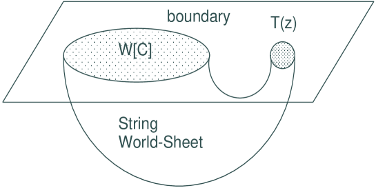
Fig. 4: We consider the two-point function $T_{\mu\nu}(z)W[C]$ in the context of AdS/CFT.

The second problem is to apply our result to the computation of the expectation value of the Wilson loop, developed by Gross and Drukker. [7] They have found that the expectation value of the Wilson loop stems from the conformal anomaly of the inversion by comparing the expectation value of a straight line and that of a circular loop. We have attempted to interpret the anomaly of the special conformal transformation, which maps a straight line into a circle, in terms of the OPE $T_{\mu\nu}(z)W[C]$. The advantage of the OPE $T_{\mu\nu}(z)W[C]$ is that this is a gauge invariant quantity. Although we have not yet obtained a definite answer, we conjecture that the undetermined coefficients $q$ and $q^{\prime}$ in the OPE (2.71) may be related to the expectation value of the Wilson loop. If we succeed in solidifying the interpretation of the conformal anomaly in terms of the OPE $T_{\mu\nu}(z)W[C]$, we may be able to gain insight into the gauge invariance of the result of Gross and Drukker.

A Proof of (2.28) $-$ (LABEL:AZ23int3+)

This appendix is devoted to the proof of the frequently used formulae concerning the spherical integral.

A.1 Integral in 3-dimensional Euclidean space

Before we consider the integral over the sphere in 4-dimensional space, we introduce the formulae concerning the integral over the surface of $S^{2}$ in 3-dimensional Euclidean space

$$z_{1}^{2}+z_{2}^{2}+z_{3}^{2}=\epsilon^{2}.$$ (A.1)

The integrals over this sphere are given by

$$(1^{\prime}) \int_{S^{2}}d\mathchar 28938\relax n_{a}=\int_{S^{2}}d\mathchar 28938\relax n_{a}z_{b}z_{c}=0,$$ (A.2)

$$(2^{\prime}) \int_{S^{2}}d\mathchar 28938\relax n_{a}z_{b}=\frac{4\pi\epsilon^{3}}{3}\delta_{ab},$$ (A.3)

$$(3^{\prime}) \int_{S^{2}}d\mathchar 28938\relax n_{a}z_{b}z_{c}z_{d}=\frac{4\pi\epsilon^{5}}{15}(\delta_{ab}\delta_{cd}+\delta_{ac}\delta_{bd}+\delta_{ad}\delta_{bc}).$$ (A.4)

Fig. 2: $y_{\mu}(u_{0})$ is the point nearest to $z_{\mu}$.

 

Here, the indices $a,b,c,\cdots$ run over $1$, $2$ and $3$, and $n^{a}$ denotes the normal vector on the sphere. These formulae are derived by noting the symmetry of the integral.

1. We first verify that the integrals (A.2) are zero. The former vanishes because of the symmetry of the sphere. For the latter integral, the result must be invariant under the $SO(3)$ rotation of the integrand, and thus the result should be

   $$\int_{S^{2}}d\mathchar 28938\relax n_{a}z_{b}z_{c}\propto\epsilon_{abc}.$$ (A.5)

   This manifestly vanishes because the integral is required to be symmetric under the exchange of $z_{b}$ and $z_{c}$.

2. The key to the derivation of the integral (A.3) is to guess the final result from the symmetry. This must give a non-zero result only when the indices satisfy $a=b$, and therefore the result is determined to be

   $$\int_{S^{2}}d\mathchar 28938\relax n_{a}z_{b}=A\delta_{ab}\int_{S^{2}}d\mathchar 28938\relax n_{c}z^{c}.$$ (A.6)

   The coefficient $A$ is determined to be $\frac{1}{3}$ by contracting the indices $a$ and $b$. And the integral on the right-hand side is evaluated using Gauss’s theorem:

   $$\int_{S^{2}}d\mathchar 28938\relax n_{a}z_{b}=\frac{1}{3}\delta_{ab}\int_{S^{2}}d\mathchar 28938\relax n^{c}z_{c}$$ (A.7)

   $$= \frac{1}{3}\delta_{ab}\int_{B^{2}}d^{3}x\overbrace{\partial^{c}z_{c}}^{=1+1+1=3}=\frac{4\pi\epsilon^{3}}{3}\delta_{ab},$$

   where $B^{2}$ denotes the region inside the sphere $S^{2}$.

3. The formula (A.4) is derived in much the same fashion. The symmetry constrains the result to be invariant under the exchange of the indices $b,c$ and $d$, and this integral is determined to be

   $$\int_{S^{2}}d\mathchar 28938\relax n_{a}z_{b}z_{c}z_{d}=A(\delta_{ab}\delta_{cd}+\delta_{ac}\delta_{bd}+\delta_{ad}\delta_{bc}).$$ (A.8)

   We are again left with the determination of the coefficient $A$. When we suppose that $a=b$ and that $c=d$, the both hand sides are rewritten as

   (l.h.s.) $$=\left(\int_{S^{2}}d\mathchar 28938\relax n_{c}z^{c}\right)\epsilon^{2}=\left(\int_{B^{2}}d^{3}x\partial^{c}z_{c}\right)\epsilon^{2}=4\pi\epsilon^{5},$$

   (r.h.s.) $$=A(\delta_{aa}\delta_{cc}+2\delta_{ac}\delta_{ac})=A(3\times 3+3+3)=15A.$$

   Therefore, the coefficient $A$ is determined to be $\frac{4\pi\epsilon^{5}}{15}$, and we obtain the result.

A.2 The integral over the enveloping surface

We next extend the previous discussion to the integral over the enveloping surface wrapping the Wilson loop in the 4-dimensional Euclidean spacetime.

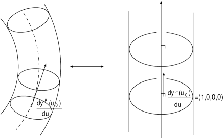
Fig. 6: We next evaluate the integral over the cylinder wrapping the Wilson loop.

In the evaluation of the conformal Ward identity, there frequently emerge the integrals (2.28) $-$ (LABEL:AZ23int3+). These are again derived by determining the forms through symmetry.

1. It is clear that the integrals (2.28) vanish by noting the symmetry of the spherical integral.

2. We verify (2.1.3) through covariance. The result should be

   $$\int_{S^{2}(u_{0})}d\mathchar 28938\relax n_{\mu}(z_{\nu}-y_{\nu}(u_{0}))=Ag_{\mu\nu}+B\frac{dy_{\mu}(u_{0})}{du}\frac{dy_{\nu}(u_{0})}{du}.$$ (A.9)

   The coefficients are determined by considering the special case. This problem is made simpler by considering the system in which the Wilson line is a straight line parameterized by

   $$y_{\mu}(u)=(u,0,0,0),$$ (A.10)

   as depicted in the right sketch in Fig. 6. The spherical integral thus reduces to the problem discussed in the previous section.

   • When $\mu=0$, this integral vanishes, because the normal vector to the sphere is always perpendicular to the tangent vector $\frac{dy_{\rho}(u_{0})}{du}$. This gives the constraint $A+B=0$ on the coefficients when $\nu$ is also 0.

   • When neither $\mu$ nor $\nu$ is $0$, this reduces to the integral (A.3), and the coefficient $A$ is determined as $A=\frac{4\pi\epsilon^{3}}{3}$.

   Therefore, the coefficients are determined as $(A,B)=(\frac{4\pi\epsilon^{3}}{3},-\frac{4\pi\epsilon^{3}}{3})$, and the result (2.1.3) is verified.

3. The integral (LABEL:AZ23int3+) is verified in the same manner, but this requires a somewhat tedious computation. It is clear that the result must be invariant under the exchange of the indices $\nu,\rho,\chi$. Also, the covariance constrains the result to be

   $$\int_{S^{2}(u_{0})}d\mathchar 28938\relax n_{\mu}(z_{\nu}-y_{\nu}(u_{0}))(z_{\rho}-y_{\rho}(u_{0}))(z_{\chi}-y_{\chi}(u_{0}))$$

   $$=A(g_{\mu\nu}g_{\rho\chi}+g_{\mu\rho}g_{\nu\chi}+g_{\mu\chi}g_{\nu\rho})+B\frac{dy_{\mu}(u_{0})}{du}\frac{dy_{\nu}(u_{0})}{du}\frac{dy_{\rho}(u_{0})}{du}\frac{dy_{\chi}(u_{0})}{du}$$

   $$+C\left(g_{\mu\nu}\frac{dy_{\rho}(u_{0})}{du}\frac{dy_{\chi}(u_{0})}{du}+g_{\mu\rho}\frac{dy_{\nu}(u_{0})}{du}\frac{dy_{\chi}(u_{0})}{du}+g_{\mu\chi}\frac{dy_{\nu}(u_{0})}{du}\frac{dy_{\rho}(u_{0})}{du}\right)$$

   $$+D\left(g_{\rho\chi}\frac{dy_{\mu}(u_{0})}{du}\frac{dy_{\nu}(u_{0})}{du}+g_{\nu\chi}\frac{dy_{\mu}(u_{0})}{du}\frac{dy_{\rho}(u_{0})}{du}+g_{\nu\rho}\frac{dy_{\mu}(u_{0})}{du}\frac{dy_{\chi}(u_{0})}{du}\right).$$

   (A.11)

   The coefficients $A,B,C$ and $D$ are again determined by considering the special case of the straight Wilson line.

   • When $\mu=0$, the result again must be zero because the $S^{2}$ sphere is perpendicular to the $z_{0}$ direction. Therefore, (A.11) must vanish if we multiply it by $\frac{dy_{\mu}(u_{0})}{du}=\delta^{\mu}_{0}$:

     $$(A+D)\left(\frac{dy_{\nu}(u_{0})}{du}g_{\rho\chi}+\frac{dy_{\rho}(u_{0})}{du}g_{\chi\nu}+\frac{dy_{\chi}(u_{0})}{du}g_{\nu\rho}\right)$$ (A.12)

     $$+ (B+3C)\frac{dy_{\nu}(u_{0})}{du}\frac{dy_{\rho}(u_{0})}{du}\frac{dy_{\chi}(u_{0})}{du}=0.$$

     This gives the constraints

     $$A+D=0,\hskip 8.53581ptB+3C=0.$$ (A.13)

   • When $\chi=0$ and $\mu,\nu,\rho=1,2,3$, this must vanish, because of the relation (A.2). In this case, (A.11) is rewritten, by multiplying $\frac{dy_{\chi}(u_{0})}{du}=\delta^{\chi}_{0}$, as

     $$A\left(g_{\mu\nu}\frac{dy_{\rho}(u_{0})}{du}+g_{\nu\rho}\frac{dy_{\mu}(u_{0})}{du}+g_{\rho\mu}\frac{dy_{\nu}(u_{0})}{du}\right)+B\frac{dy_{\mu}(u_{0})}{du}\frac{dy_{\nu}(u_{0})}{du}\frac{dy_{\rho}(u_{0})}{du}$$ (A.14)

     $$+ C\left(g_{\mu\nu}\frac{dy_{\rho}(u_{0})}{du}+g_{\mu\rho}\frac{dy_{\nu}(u_{0})}{du}+\frac{dy_{\mu}(u_{0})}{du}\frac{dy_{\nu}(u_{0})}{du}\frac{dy_{\rho}(u_{0})}{du}\right)$$

     $$+ D\left(2\frac{dy_{\mu}(u_{0})}{du}\frac{dy_{\nu}(u_{0})}{du}\frac{dy_{\rho}(u_{0})}{du}+g_{\rho\nu}\frac{dy_{\mu}(u_{0})}{du}\right)=0.$$

     The coefficients are thus constrained to be

     $$-A=C=D,\hskip 8.53581ptB+C+2D=0.$$ (A.15)

   • Finally, we consider the case in which neither of the indices are $0$. In this case, $A$ is determined by identifying this case with the integral (A.4): $A=\frac{4\pi\epsilon^{5}}{15}$.

   The coefficients in (A.11) are thus determined to be

   $$(A,B,C,D)=\left(\frac{4\pi\epsilon^{5}}{15},\frac{4\pi\epsilon^{5}}{5},-\frac{4\pi\epsilon^{5}}{15},-\frac{4\pi\epsilon^{5}}{15}\right).$$ (A.16)

B Proof of (2.46)

In this appendix, we present the explicit computation of the deformation of the Wilson loop (2.46). We deform the loop slightly as

$$y_{\mu}(s)\to y_{\mu}(s)+\delta y_{\mu}(s).$$ (B.1)

Fig. 7: The deformation of the loop.

The Wilson loop varies under this deformation as

$$W[C] \to \frac{1}{N}\textrm{Tr}P\exp\left[\int^{2\pi}_{0}ds\left\{iA_{\mu}(y(s)+\delta y(s))\frac{d(y^{\mu}+\delta y^{\mu}(s))}{ds}\right.\right.$$

$$\hskip 14.22636pt+\left.\left.|\frac{d}{ds}(y_{\mu}(s)+\delta y_{\mu}(s))|\theta_{i}(s)\phi^{i}(y(s)+\delta y(s))\right\}\right]$$

$$= \frac{1}{N}\textrm{Tr}P\exp\left[\int^{2\pi}_{0}ds\left\{iA_{\mu}(y(s))\frac{dy^{\mu}(s)}{ds}+i(\partial_{\nu}A_{\mu}(y(s)))\frac{dy^{\mu}(s)}{ds}\delta y^{\nu}(s)\right.\right.$$

$$\hskip 14.22636pt+iA_{\nu}(y(s))\frac{d(\delta y^{\nu}(s))}{ds}+\theta_{i}(s)\phi^{i}(y(s))|\frac{dy_{\mu}(s)}{ds}|$$

$$\hskip 14.22636pt+\theta_{i}(s)(\partial_{\nu}\phi^{i}(y(s)))|\frac{dy_{\mu}(s)}{ds}|\delta y^{\nu}(s)$$

$$\hskip 14.22636pt+\left.\theta_{i}(s)\phi^{i}(y(s))\frac{1}{|\frac{dy_{\mu}(s)}{ds}|}\frac{dy_{\nu}(s)}{ds}\left(\frac{d(\delta y^{\nu}(s))}{ds}\right)\Bigr{\}}\right]$$

$$= W[C]+\int^{2\pi}_{0}ds\delta y^{\nu}(s)\textrm{Tr}P{\hat{w}}_{2\pi,s}\left[i(\partial_{\nu}A_{\alpha}(y(s)))\frac{dy^{\alpha}(s)}{ds}\right.$$

$$\hskip 14.22636pt+\left.\theta_{i}(s)(\partial_{\nu}\phi^{i}(y(s)))|\frac{dy_{\mu}(s)}{ds}|\right]{\hat{w}}_{s,0}$$

$$-\frac{1}{N}\int^{2\pi}_{0}ds\delta y^{\nu}(s)\left[\frac{d}{ds}\left\{\textrm{Tr}P({\hat{w}}_{2\pi,s}iA_{\nu}(y(s)){\hat{w}}_{s,0})\right\}\right]$$

$$-\frac{1}{N}\int^{2\pi}_{0}ds\delta y^{\nu}(s)\left[\frac{d}{ds}\left\{\textrm{Tr}P\left({\hat{w}}_{2\pi,s}\theta_{i}(s)\phi^{i}(y(s))\frac{1}{|\frac{dy_{\mu}(s)}{ds}|}\frac{dy_{\nu}(s)}{ds}{\hat{w}}_{s,0}\right)\right\}\right]$$

$$= W[C]+\frac{1}{N}\int^{2\pi}_{0}ds\delta y^{\nu}(s)\textrm{Tr}P{\hat{w}}_{2\pi,s}\left[iF_{\nu\alpha}(y(s))\frac{dy^{\alpha}(s)}{ds}+\theta_{i}(s)|\frac{dy_{\mu}(s)}{ds}|D_{\nu}\phi^{i}(y(s))\right]{\hat{w}}_{s,0}$$

$$-\frac{1}{N}\int^{2\pi}_{0}ds\delta y^{\nu}(s)\left[\frac{d}{ds}\left\{\textrm{Tr}P\left({\hat{w}}_{2\pi,s}\theta_{i}(s)\phi^{i}(y(s))\frac{1}{|\frac{dy_{\mu}(s)}{ds}|}\frac{dy_{\nu}(s)}{ds}{\hat{w}}_{s,0}\right)\right\}\right].$$

We thus obtain the deformation of the Wilson loop as

$$\left(\frac{\delta W[C]}{\delta y^{\nu}(s)}\right) = \frac{1}{N}\textrm{Tr}P{\hat{w}}_{2\pi,s}\left[iF_{\nu\alpha}(y(s))\frac{dy^{\alpha}(s)}{ds}+|\frac{dy_{\mu}(s)}{ds}|\theta_{i}(s)D_{\nu}\phi^{i}(y(s))\right]{\hat{w}}_{s,0}$$

$$- \frac{d}{ds}\left[\frac{1}{N}\textrm{Tr}P{\hat{w}}_{2\pi,s}\left\{\theta_{i}(s)\phi^{i}(y(s))\frac{\frac{dy_{\nu}(s)}{ds}}{|\frac{dy_{\mu}(s)}{ds}|}\right\}{\hat{w}}_{s,0}\right].$$

C Proof of (3.2)

This appendix provides a quick proof of the energy-momentum tensor of the $U(1)$ SYM theory, as an example of enjoying an advantage of the scale invariance and the conservation law of the energy-momentum tensor. The result (3.2) can be obtained by differentiating the scalar curvature with respect to the metric. Here, we take a shortcut by imposing the following ansatz instead:

$$\frac{2}{\sqrt{g}}\frac{-\frac{1}{12G^{2}}\sqrt{g}R\phi_{i}(z)\phi^{i}(z)}{\partial g^{\mu\nu}}|_{\textrm{flat space}}$$ (C.1)

$$= \frac{1}{G^{2}}[A\partial_{\mu}\partial_{\nu}(\phi_{i}(z)\phi^{i}(z))+Bg_{\mu\nu}\Box(\phi_{i}(z)\phi^{i}(z))].$$

The coefficients $A$ and $B$ should be determined by the tracelessness and divergencelessness condition of the energy-momentum tensor. The energy-momentum tensor in the Euclidean flat space is

$$T_{\mu\nu}(z) = \frac{2}{\sqrt{g}}\frac{\partial{\cal L}}{\partial g^{\mu\nu}}=\frac{1}{G^{2}}\left[F_{\mu\alpha}(z){F_{\nu}}^{\alpha}(z)-\frac{1}{4}g_{\mu\nu}F_{\alpha\beta}(z)F^{\alpha\beta}(z)\right.$$ (C.2)

$$+(\partial_{\mu}\phi_{i}(z))(\partial_{\nu}\phi^{i}(z))-\frac{1}{2}g_{\mu\nu}(\partial_{\lambda}\phi_{i}(z))(\partial^{\lambda}\phi^{i}(z))$$

$$+\left.A\partial_{\mu}\partial_{\nu}(\phi_{i}(z)\phi^{i}(z))+Bg_{\mu\nu}\Box(\phi_{i}(z)\phi^{i}(z))\right].$$

These two fundamental properties of the energy momentum tensor impose the following constraints on the unknown coefficients.

• ${T_{\mu}}^{\mu}(z)=0$: This gives the relation $2A+8B-1=0$, with the help of the Klein-Gordon equation $\Box\phi_{i}(z)=0$.

• $\partial^{\mu}T_{\mu\nu}(z)=0$: This leads to the constraint $A+B=0$.

The coefficients are determined as $A=-\frac{1}{6}$ and $B=\frac{1}{6}$, and this completes the proof of (3.2).

D Proof of (3.7) $-$ (3.7)

This appendix is devoted to the explicit computation of the OPE $T_{\mu\nu}(z)W[C]$ in the $U(1)$ SYM theory. We first take contractions following Wick’s theorem. Then, we obtain

$$T_{\mu\nu}(z)W[C]=(T_{\mu\nu}(z)W[C])_{\textrm{c}}+(T_{\mu\nu}(z)W[C])_{\textrm{vec}}+(T_{\mu\nu}(z)W[C])_{\textrm{sca}}.$$

Here, $(T_{\mu\nu}(z)W[C])_{\textrm{c}}$ represents the result of two contractions, while $(T_{\mu\nu}(z)W[C])_{\textrm{vec}}$ and $(T_{\mu\nu}(z)W[C])_{\textrm{sca}}$ represent the results of the single contraction with respect to the vector and scalar fields, respectively. The explicit form of each component is given below.

$$(T_{\mu\nu}(z)W[C])_{\textrm{c}} = G^{2}\oint_{C}du^{\prime}du^{\prime\prime}[-(\partial_{\alpha}D(z-y(u^{\prime})))(\partial^{\alpha}D(z-y(u^{\prime\prime}))){\dot{y}}_{\mu}(y^{\prime}){\dot{y}}_{\nu}(u^{\prime\prime})$$ (D.2)

$$-(\partial_{\mu}D(z-y(u^{\prime})))(\partial_{\nu}D(z-y(u^{\prime\prime}))){\dot{y}}_{\alpha}(u^{\prime}){\dot{y}}^{\alpha}(u^{\prime\prime})$$

$$+(\partial_{\alpha}D(z-y(u^{\prime})))(\partial_{\nu}D(z-y(u^{\prime\prime}))){\dot{y}}_{\mu}(u^{\prime}){\dot{y}}^{\alpha}(u^{\prime\prime})$$

$$+(\partial_{\mu}D(z-y(u^{\prime})))(\partial^{\alpha}D(z-y(u^{\prime\prime}))){\dot{y}}_{\alpha}(u^{\prime}){\dot{y}}_{\nu}(u^{\prime\prime})$$

$$+\frac{g_{\mu\nu}}{2}(\partial^{\beta}D(z-y(u^{\prime})))(\partial_{\beta}D(z-y(u^{\prime\prime}))){\dot{y}}_{\alpha}(u^{\prime}){\dot{y}}^{\alpha}(u^{\prime\prime})$$

$$-\frac{g_{\mu\nu}}{2}(\partial_{\alpha}D(z-y(u^{\prime})))(\partial_{\beta}D(z-y(u^{\prime\prime}))){\dot{y}}^{\alpha}(u^{\prime\prime}){\dot{y}}^{\beta}(u^{\prime})]W[C]$$

$$+G^{2}\oint_{C}du^{\prime}du^{\prime\prime}\theta_{k}(u^{\prime})\theta^{k}(u^{\prime\prime})\left[\frac{1}{3}(\partial_{\mu}D(z-y(u^{\prime})))(\partial_{\nu}D(z-y(u^{\prime\prime})))\right.$$

$$+\frac{1}{3}(\partial_{\nu}D(z-y(u^{\prime})))(\partial_{\mu}D(z-y(u^{\prime\prime})))$$

$$-\frac{g_{\mu\nu}}{6}(\partial_{\alpha}D(z-y(u^{\prime})))(\partial^{\alpha}D(z-y(u^{\prime\prime})))$$

$$-\frac{1}{6}[D(z-y(u^{\prime}))(\partial_{\mu}\partial_{\nu}D(z-y(u^{\prime\prime})))+D(z-y(u^{\prime\prime}))(\partial_{\mu}\partial_{\nu}D(z-y(u^{\prime})))]$$

$$+\frac{1}{6}g_{\mu\nu}[D(z-y(u^{\prime}))(\delta(z-y(u^{\prime\prime})))$$

$$+\left.D(z-y(u^{\prime\prime}))(\delta(z-y(u^{\prime})))]\right]W[C],$$

$$(T_{\mu\nu}(z)W[C])_{\textrm{vec}} = i\left[\oint_{C}du(-(\partial_{\mu}D(z-y(u)))F_{\nu\alpha}(y(u)){\dot{y}}^{\alpha}(u)\right.$$ (D.3)

$$-(\partial_{\nu}D(z-y(u)))F_{\mu\alpha}(y(u)){\dot{y}}^{\alpha}(u)$$

$$+g_{\mu\nu}(\partial^{\alpha}D(z-y(u)))F_{\alpha\beta}(y(u)){\dot{y}}^{\beta}(u)$$

$$\left.+(\partial^{\alpha}D(z-y(u)))(F_{\mu\alpha}(y(u)){\dot{y}}_{\nu}(u)+F_{\nu\alpha}(y(u)){\dot{y}}_{\mu}(u)))\right]W[C],$$

$$(T_{\mu\nu}(z)W[C])_{\textrm{sca}} = \oint_{C}du\frac{1}{3}\theta^{i}(u)\left[\phi_{i}(y(u))(\partial_{\mu}\partial_{\nu}D(z-y(u)))\right.$$ (D.4)

$$-\left.\frac{1}{3}g_{\mu\nu}\phi_{i}(y(u))\delta(z-y(u))\right]W[C]$$

$$+\oint_{C}du\theta^{i}(u)\left[-\frac{2}{3}(\partial_{\mu}D(z-y(u)))(\partial_{\nu}\phi_{i}(y(u)))-\frac{2}{3}(\partial_{\nu}D(z-y(u)))(\partial_{\mu}\phi_{i}(y(u)))\right.$$

$$+\frac{g_{\mu\nu}}{3}(\partial_{\alpha}D(z-y(u)))(\partial^{\alpha}\phi_{i}(y(u)))$$

$$+\frac{1}{3}(\partial^{\alpha}\phi_{i}(y(u)))(z_{\alpha}-y_{\alpha}(u))(\partial_{\mu}\partial_{\nu}D(z-y(u)))$$

$$\left.+\frac{1}{3}g_{\mu\nu}(\partial^{\alpha}\phi_{i}(y(u)))(z_{\alpha}-y_{\alpha}(u))\delta(z-y(u))\right]W[C].$$

In this appendix, the dotted quantities represents derivatives with respect to the arc length parameter: ${\dot{y}}_{\mu}(u)=\frac{dy_{\mu}(u)}{du}$, ${\ddot{y}}_{\mu}(u)=\frac{d^{2}y_{\mu}(u)}{du^{2}}$, and so on. Also, we define $D(z-y(u))=\frac{-1}{4\pi^{2}(z-y(u))^{2}}$.

We next perform the integral over the Wilson loop. We expand the quantities around the point $y_{\mu}(u_{0})$, the nearest point on the Wilson loop to $z_{\mu}$. The miscellaneous quantities in the integral are expanded as follows:

$$y_{\mu}(u) = y_{\mu}(u_{0})+(u-u_{0}){\dot{y}}_{\mu}(u_{0})+\frac{(u-u_{0})^{2}}{2}{\ddot{y}}_{\mu}(u_{0})+\cdots,$$ (D.5)

$$\theta_{i}(u) = \theta_{i}(u_{0})+(u-u_{0}){\dot{\theta}}_{i}(u_{0})+\frac{(u-u_{0})^{2}}{2}{\ddot{\theta}_{i}}(u_{0})+\cdots,$$ (D.6)

$$\frac{1}{(z-y(u))^{2n}} = \left[(z_{\mu}-y_{\mu}(u_{0})-(u-u_{0}){\dot{y}}_{\mu}(u_{0})-\frac{(u-u_{0})^{2}}{2}{\ddot{y}}_{\mu}(u_{0})-\cdots)^{2}\right]^{-n}$$ (D.7)

$$= [(z_{\mu}-y_{\mu}(u_{0}))^{2}+(u-u_{0})^{2}]^{-n}$$

$$\times\left[1-\frac{(u-u_{0})^{2}(z_{\mu}-y_{\mu}(u_{0})){\ddot{y}}^{\mu}(u_{0})}{[(z_{\mu}-y_{\mu}(u_{0}))^{2}+(u-u_{0})^{2}]}-\cdots\right]^{-n}$$

$$= \frac{1}{[(z_{\mu}-y_{\mu}(u_{0}))^{2}+(u-u_{0})^{2}]^{n}}$$

$$+ \frac{n(u-u_{0})^{2}(z_{\mu}-y_{\mu}(u_{0})){\ddot{y}}^{\mu}(u_{0})}{[(z_{\mu}-y_{\mu}(u_{0}))^{2}+(u-u_{0})^{2}]^{n+1}}+\cdots.$$

The expansion of the denominator (D.7) needs some explanation.

• We expand the denominator $\frac{1}{(z-y(u))^{2n}}$ around

  $$\frac{1}{[(z_{\mu}-y_{\mu}(u_{0}))^{2}+(u-u_{0})^{2}]^{n}},$$

  because we approximate the integration over the Wilson loop by the integral over the straight line. In analyzing the conformal Ward identity, the point $z_{\mu}$ is on the $S^{2}(u_{0})$ sphere whose radius is $\epsilon$, and the point $z_{\mu}$ is in the vicinity of the Wilson loop. Therefore, the Wilson loop is perceived as a straight line, just as we perceive the earth as a flat plane because the earth is much bigger than we are.

• In this expansion, we must be careful about the fact that ${\dot{y}}_{\alpha}(u_{0}){\ddot{y}}^{\alpha}(u_{0})=\frac{1}{2}(\frac{d}{du}|{\dot{y}}_{\alpha}(u_{0})|^{2})=0$ and that the definition of the point $y_{\mu}(u_{0})$ immediately leads to $(z_{\mu}-y_{\mu}(u_{0})){\dot{y}}^{\mu}(u_{0})=0$.

The following integral is useful in the computation given below:

$$\int^{+\infty}_{-\infty}du\frac{(u-u_{0})^{n}}{2\pi^{2}((u-u_{0})^{2}+(z_{\mu}-y_{\mu}(u_{0}))^{2})^{m}}$$ (D.10)

$$= \{\begin{array}[]{ll}0&(n\textrm{ is an odd number.})\\ \frac{(n-1)!!(2m-n-3)!!}{2\pi|z_{\mu}-y_{\mu}(u_{0})|^{2m-n-1}(2m-2)!!}&(n\textrm{ is an even number.})\end{array},$$

where $m$ and $n$ are positive integers satisfying $2m>n$. We now give the computation for deriving the formula (3.7) $-$ (3.7). The computation is rather lengthy, and we compute the terms one by one.

D.1 The computation of $(T_{\mu\nu}(z)W[C])_{\textrm{c}}$

Since this is a contribution of $W[C]$ itself, it suffices to perform the computation to ${\cal O}(z-y(u_{0}))^{-3}$. We have already shown that the terms of ${\cal O}(z-y(u_{0}))^{-2}$ do not contribute to the conformal Ward identity. The following quantities are frequently involved in the computation:

$$\int^{+\infty}_{-\infty}du{\dot{y}}_{\nu}(u)(\partial_{\mu}D(z-y(u)))=O_{\mu\nu}^{-2}+O_{\mu\nu}^{-1}+\cdots,$$

$$\int^{+\infty}_{-\infty}du\theta_{i}(u)(\partial_{\mu}D(z-y(u)))=P_{\mu}^{-2}+P^{-1}_{\mu}+\cdots,$$

$$\int^{+\infty}_{-\infty}du\theta_{i}(u)D(z-y(u))=P^{-1}+P^{0}+\cdots,$$

$$\int^{+\infty}_{-\infty}du\theta_{i}(u)(\partial_{\mu}\partial_{\nu}D(z-y(u)))=P^{-3}_{\mu\nu}+P^{-2}_{\mu\nu}+\cdots,\textrm{ where}$$

$$O^{-2}_{\mu\nu} = \frac{(z_{\mu}-y_{\mu}(u_{0})){\dot{y}}_{\nu}(u_{0})}{4\pi|z-y(u_{0})|^{3}},$$ (D.11)

$$O^{-1}_{\mu\nu} = \frac{[(z_{\alpha}-y_{\alpha}(u_{0})){\ddot{y}}^{\alpha}(u_{0})](z_{\mu}-y_{\mu}(u_{0})){\dot{y}}_{\nu}(u_{0})}{8\pi|z-y(u_{0})|^{3}}$$ (D.12)

$$-\frac{{\dot{y}}_{\mu}(u_{0}){\ddot{y}}_{\nu}(u_{0})+\frac{1}{2}{\ddot{y}}_{\mu}(u_{0}){\dot{y}}_{\nu}(u_{0})}{4\pi|z-y(u_{0})|},$$

$$P_{\mu}^{-2} = \frac{(z_{\mu}-y_{\mu}(u_{0}))\theta_{i}(u_{0})}{4\pi|z-y(u_{0})|^{3}},$$ (D.13)

$$P_{\mu}^{-1} = \frac{[(z_{\alpha}-y_{\alpha}(u_{0}))\cdot{\ddot{y}}^{\alpha}(u_{0})](z_{\mu}-y_{\mu}(u_{0}))\theta_{i}(u_{0})}{8\pi|z-y(u_{0})|^{3}}$$ (D.14)

$$-\frac{{\ddot{y}}_{\mu}(u_{0})\theta_{i}(u_{0})}{8\pi|z-y(u_{0})|}-\frac{{\dot{y}}_{i}(u_{0}){\dot{\theta}}_{i}(u_{0})}{4\pi|z-y(u_{0})|},$$

$$P^{-1} = -\frac{\theta_{i}(u_{0})}{4\pi|z-y(u_{0})|},$$

$$P^{0} = -\frac{\theta_{i}(u_{0})[(z_{\alpha}-y_{\alpha}(u_{0})){\ddot{y}}^{\alpha}(u_{0})]}{8\pi|z-y(u_{0})|},$$ (D.15)

$$P^{-3}_{\mu\nu} = -\frac{3(z_{\mu}-y_{\mu}(u_{0}))(z_{\nu}-y_{\nu}(u_{0}))\theta_{i}(u_{0})}{4\pi|z-y(u_{0})|^{5}}$$ (D.16)

$$-\frac{{\dot{y}}_{\mu}(u_{0}){\dot{y}}_{\nu}(u_{0})\theta_{i}(u_{0})}{4\pi|z-y(u_{0})|^{3}}+g_{\mu\nu}\frac{\theta_{i}(u_{0})}{4\pi|z-y(u_{0})|^{3}},$$

$$P^{-2}_{\mu\nu} = -\frac{3\theta_{i}(u_{0})(z_{\mu}-y_{\mu}(u_{0}))(z_{\nu}-y_{\nu}(u_{0}))[(z_{\alpha}-y_{\alpha}(u_{0})){\ddot{y}}^{\alpha}(u_{0})]}{8\pi|z-y(u_{0})|^{5}}$$ (D.17)

$$+\frac{{\dot{\theta}}_{i}(u_{0})[(z_{\mu}-y_{\mu}(u_{0})){\dot{y}}_{\nu}(u_{0})+(z_{\nu}-y_{\nu}(u_{0})){\dot{y}}_{\mu}(u_{0})]}{4\pi|z-y(u_{0})|^{3}}$$

$$-\frac{3\theta_{i}(u_{0})[(z_{\alpha}-y_{\alpha}(u_{0})){\ddot{y}}^{\alpha}(u_{0})]{\dot{y}}_{\mu}(u_{0}){\dot{y}}_{\nu}(u_{0})}{8\pi|z-y(u_{0})|^{3}}$$

$$+\frac{\theta_{i}(u_{0})[(z_{\mu}-y_{\mu}(u_{0})){\ddot{y}}_{\nu}(u_{0})+(z_{\nu}-y_{\nu}(u_{0})){\ddot{y}}_{\nu}(u_{0})]}{8\pi|z-y(u_{0})|^{3}}$$

$$+g_{\mu\nu}\frac{\theta_{i}(u_{0})[(z_{\alpha}-y_{\alpha}(u_{0})){\ddot{y}}^{\alpha}(u_{0})]}{8\pi|z-y(u_{0})|^{3}}.$$

Each term of (D.2) is thus integrated as follows:

$$-G^{2}\left[\oint_{C}du^{\prime}du^{\prime\prime}(\partial_{\alpha}D(z-y(u^{\prime})))(\partial^{\alpha}D(z-y(u^{\prime\prime}))){\dot{y}}_{\mu}(u^{\prime}){\dot{y}}_{\nu}(u^{\prime\prime})\right]W[C]$$

$$= -G^{2}({O^{-2\alpha}}_{\mu}+{O^{-1\alpha}}_{\mu}+\cdots)(O^{-2}_{\alpha\nu}+O^{-1}_{\alpha\nu}+\cdots)W[C]$$

$$= -G^{2}({O^{-2\alpha}}_{\mu}O^{-2}_{\alpha\nu})W[C]-G^{2}({O^{-2\alpha}}_{\mu}O^{-1}_{\alpha\nu}+{O^{-2\alpha}}_{\nu}O^{-1}_{\alpha\mu})W[C]+\cdots$$

$$= -\frac{G^{2}}{16\pi^{2}}\frac{{\dot{y}}_{\mu}(u_{0}){\dot{y}}_{\nu}(u_{0})}{|z-y(u_{0})|^{4}}W[C]+{\cal O}(z-y(u_{0}))^{-2},$$

$$-G^{2}\left[\oint_{C}du^{\prime}du^{\prime\prime}(\partial_{\mu}D(z-y(u^{\prime})))(\partial_{\nu}D(z-y(u^{\prime\prime}))){\dot{y}}_{\alpha}(u^{\prime}){\dot{y}}^{\alpha}(u^{\prime\prime})\right]W[C]$$

$$= -G^{2}({{O^{-2}}_{\mu}}^{\alpha}O^{-2}_{\nu\alpha})W[C]-G^{2}({{O^{-2}}_{\mu}}^{\alpha}O^{-1}_{\nu\alpha}+{{O^{-2}}_{\nu}}^{\alpha}O^{-1}_{\mu\alpha})W[C]+\cdots$$

$$= \left[-\frac{G^{2}}{16\pi^{2}}\frac{(z_{\mu}-y_{\mu}(u_{0}))(z_{\nu}-y_{\nu}(u_{0}))}{|z-y(u_{0})|^{6}}\right.$$

$$-\frac{G^{2}}{16\pi^{2}}\frac{(z_{\alpha}-y_{\alpha}(u_{0})){\ddot{y}}^{\alpha}(u_{0})(z_{\mu}-y_{\mu}(u_{0}))(z_{\nu}-y_{\nu}(u_{0}))}{|z-y(u_{0})|^{6}}$$

$$+\left.\frac{G^{2}}{32\pi^{2}}\frac{(z_{\mu}-y_{\mu}(u_{0})){\ddot{y}}_{\nu}(u_{0})+(z_{\nu}-y_{\nu}(u_{0})){\ddot{y}}_{\mu}(u_{0})}{|z-y(u_{0})|^{4}}\right]W[C]$$

$$+{\cal O}(z-y(u_{0}))^{-2},$$

$$G^{2}\left[\oint_{C}du^{\prime}du^{\prime\prime}[(\partial_{\alpha}D(z-y(u^{\prime})))(\partial_{\nu}D(z-y(u^{\prime\prime}))){\dot{y}}_{\mu}(u^{\prime}){\dot{y}}^{\alpha}(u^{\prime\prime})\right.$$

$$\hskip 14.22636pt+\left.(\partial_{\mu}D(z-y(u^{\prime})))(\partial^{\alpha}D(z-y(u^{\prime\prime}))){\dot{y}}_{\alpha}(u^{\prime}){\dot{y}}_{\nu}(u^{\prime\prime})]\right]W[C]$$

$$= [G^{2}({O^{-2\alpha}}_{\mu}O^{-2}_{\nu\alpha})+G^{2}({O^{-2\alpha}}_{\mu}O^{-1}_{\nu\alpha}+{{O^{-2}}_{\nu}}^{\alpha}O^{-1}_{\alpha\mu})$$

$$\hskip 14.22636pt+G^{2}({O^{-2\alpha}}_{\nu}O^{-2}_{\mu\alpha})+G^{2}({O^{-2\alpha}}_{\nu}O^{-1}_{\mu\alpha}+{{O^{-2}}_{\mu}}^{\alpha}O^{-1}_{\alpha\nu})]W[C]+\cdots$$

$$= \left[-\frac{G^{2}}{8\pi^{2}}\frac{((z_{\alpha}-y_{\alpha}(u_{0})){\ddot{y}}^{\alpha}(u_{0})){\dot{y}}_{\mu}(u_{0}){\dot{y}}_{\nu}(u_{0})}{|z-y(u_{0})|^{4}}\right.$$

$$-\left.\frac{G^{2}}{16\pi^{2}}\frac{(z_{\mu}-y_{\mu}(u_{0})){\ddot{y}}_{\nu}(u_{0})+(z_{\nu}-y_{\nu}(u_{0})){\ddot{y}}_{\mu}(u_{0})}{|z-y(u_{0})|^{4}}\right]W[C]$$

$$+{\cal O}(z-y(u_{0}))^{-2},$$

$$\frac{G^{2}}{2}\left[\oint_{C}du^{\prime}du^{\prime\prime}g_{\mu\nu}(\partial^{\beta}D(z-y(u^{\prime})))(\partial_{\beta}D(z-y(u^{\prime\prime}))){\dot{y}}_{\alpha}(u^{\prime}){\dot{y}}^{\alpha}(u^{\prime\prime})\right]W[C]$$

$$= \frac{G^{2}}{2}g_{\mu\nu}[(O^{-2}_{\alpha\beta}O^{-2\alpha\beta})+2(O^{-2}_{\alpha\beta}O^{-1\alpha\beta})]W[C]+\cdots$$

$$= \frac{G^{2}}{32\pi^{2}}\frac{g_{\mu\nu}}{|z-y(u_{0})|^{4}}W[C]+{\cal O}(z-y(u_{0}))^{-2},$$

$$-\frac{G^{2}}{2}\left[\oint_{C}du^{\prime}du^{\prime\prime}g_{\mu\nu}(\partial_{\alpha}D(z-y(u^{\prime})))(\partial_{\beta}D(z-y(u^{\prime\prime}))){\dot{y}}^{\alpha}(u^{\prime\prime}){\dot{y}}^{\beta}(u^{\prime})\right]W[C]$$

$$= -\frac{G^{2}}{2}g_{\mu\nu}[(O^{-2}_{\alpha\beta}O^{-2\beta\alpha})+2(O^{-2}_{\alpha\beta}O^{-1\beta\alpha})]W[C]+\cdots$$

$$= \frac{G^{2}}{16\pi^{2}}g_{\mu\nu}\frac{(z_{\alpha}-y_{\alpha}(u_{0})){\ddot{y}}^{\alpha}(u_{0})}{|z-y(u_{0})|^{4}}W[C]+{\cal O}(z-y(u_{0}))^{-2},$$

$$\frac{G^{2}}{3}\left[\oint_{C}du^{\prime}du^{\prime\prime}\theta_{i}(u^{\prime})\theta^{i}(u^{\prime\prime})[(\partial_{\mu}D(z-y(u^{\prime})))(\partial_{\nu}D(z-y(u^{\prime\prime})))\right.$$

$$\hskip 14.22636pt+\left.(\partial_{\nu}D(z-y(u^{\prime})))(\partial_{\mu}D(z-y(u^{\prime\prime})))]\right]W[C]$$

$$= \frac{2G^{2}}{3}(P^{-2}_{\mu}+P^{-1}_{\mu}+\cdots)(P^{-2}_{\nu}+P^{-1}_{\nu}+\cdots)W[C]$$

$$= \frac{2G^{2}}{3}[(P^{-2}_{\mu}P^{-2}_{\nu})+(P^{-2}_{\mu}P^{-1}_{\nu}+P^{-2}_{\nu}P^{-1}_{\mu})+\cdots]W[C]$$

$$= \left[\frac{G^{2}}{24\pi^{2}}\frac{(z_{\mu}-y_{\mu}(u_{0}))(z_{\nu}-y_{\nu}(u_{0}))}{|z_{\mu}-y_{\mu}(u_{0})|^{6}}\right.$$

$$+\frac{G^{2}}{24\pi^{2}}\frac{[(z_{\alpha}-y_{\alpha}(u_{0})){\ddot{y}}^{\alpha}(u_{0})](z_{\mu}-y_{\mu}(u_{0}))(z_{\nu}-y_{\nu}(u_{0}))}{|z-y(u_{0})|^{6}}$$

$$-\left.\frac{G^{2}}{48\pi^{2}}\frac{(z_{\mu}-y_{\mu}(u_{0})){\ddot{y}}_{\nu}(u_{0})+(z_{\nu}-y_{\nu}(u_{0})){\ddot{y}}_{\mu}(u_{0})}{|z-y(u_{0})|^{4}}\right]W[C]$$

$$+{\cal O}(z-y(u_{0}))^{-2},$$

$$-\frac{G^{2}}{6}\left[\oint_{C}du^{\prime}du^{\prime\prime}g_{\mu\nu}\theta_{i}(u^{\prime})\theta^{i}(u^{\prime\prime})(\partial_{\alpha}D(z-y(u^{\prime})))(\partial^{\alpha}D(z-y(u^{\prime\prime})))\right]W[C]$$

$$= -\frac{G^{2}}{6}g_{\mu\nu}(P^{-2}_{\alpha}+P^{-1}_{\alpha}+\cdots)(P^{-2\alpha}+P^{-1\alpha}+\cdots)W[C]$$

$$= -\frac{G^{2}}{6}g_{\mu\nu}[(P^{-2}_{\alpha}P^{-2\alpha})+(2P^{-2}_{\alpha}P^{-1\alpha})]W[C]+\cdots$$

$$= -\frac{G^{2}}{96\pi^{2}}g_{\mu\nu}\frac{1}{|z-y(u_{0})|^{4}}W[C]+{\cal O}(z-y)^{-2},$$ (D.25)

$$-\frac{G^{2}}{6}\left[\oint_{C}du^{\prime}du^{\prime\prime}\theta_{i}(u^{\prime})\theta^{i}(u^{\prime\prime})[D(z-y(u^{\prime}))(\partial_{\mu}\partial_{\nu}D(z-y(u^{\prime\prime})))\right.$$

$$\hskip 14.22636pt+\left.D(z-y(u^{\prime\prime}))(\partial_{\mu}\partial_{\nu}D(z-y(u^{\prime})))]\right]W[C]$$

$$= -\frac{G^{2}}{3}(P^{-1}+P^{0}+\cdots)(P^{-3}_{\mu\nu}+P^{-2}_{\mu\nu}+\cdots)W[C]$$

$$= -\frac{G^{2}}{3}[(P^{-1}P^{-3}_{\mu\nu})+(P^{0}P^{-3}_{\mu\nu}+P^{-1}P^{-2}_{\mu\nu})]W[C]+\cdots$$

$$= \left[\frac{G^{2}}{48\pi^{2}}\left[-3\frac{(z_{\mu}-y_{\mu}(u_{0}))(z_{\nu}-y_{\nu}(u_{0}))}{|z-y(u_{0})|^{6}}-\frac{{\dot{y}}_{\mu}(u_{0}){\dot{y}}_{\nu}(u_{0})}{|z-y(u_{0})|^{4}}+g_{\mu\nu}\frac{1}{|z-y(u_{0})|^{4}}\right]\right.$$

$$-\frac{G^{2}}{16\pi^{2}}\frac{(z_{\mu}-y_{\mu}(u_{0}))(z_{\nu}-y_{\nu}(u_{0}))[(z_{\alpha}-y_{\alpha}(u_{0})){\ddot{y}}^{\alpha}(u_{0})]}{|z-y(u_{0})|^{6}}$$

$$-\frac{G^{2}}{24\pi^{2}}\frac{[(z_{\alpha}-y_{\alpha}(u_{0})){\ddot{y}}^{\alpha}(u_{0})]{\dot{y}}_{\mu}(u_{0}){\dot{y}}_{\nu}(u_{0})}{|z-y(u_{0})|^{4}}$$

$$+\frac{G^{2}}{96\pi^{2}}\frac{(z_{\mu}-y_{\mu}(u_{0})){\ddot{y}}_{\nu}(u_{0})+(z_{\nu}-y_{\nu}(u_{0})){\ddot{y}}_{\mu}(u_{0})}{|z-y(u_{0})|^{4}}$$

$$+\left.\frac{G^{2}}{48\pi^{2}}g_{\mu\nu}\frac{(z_{\alpha}-y_{\alpha}(u_{0})){\ddot{y}}^{\alpha}(u_{0})}{|z-y(u_{0})|^{4}}\right]W[C]+{\cal O}(z-y(u_{0}))^{-2}.$$

Above, we have utilized the fact that the term $\theta_{i}(u_{0}){\dot{\theta}}^{i}(u_{0})$ vanishes because we have set $\theta_{i}(u_{0})\theta^{i}(u_{0})=1$. Summing all of the these terms, we obtain the result (3.7).

D.2 The computation of $(T_{\mu\nu}(z)W[C])_{\textrm{vec}}$

This computation is trivial, because the singularity of the integrand is ${\cal O}(z-y(u))^{-3}$. Only the leading term in the expansion around the nearest point survives, and we can trivially read off the result (LABEL:AZ22vecres).

D.3 The computation of $(T_{\mu\nu}(z)W[C])_{\textrm{sca}}$

We next compute the effect of the scalar field. The following three terms are computed as easily as those of the vector field:

$$\oint_{C}du\theta^{i}(u)\left[-\frac{2}{3}(\partial_{\mu}D(z-y(u)))(\partial_{\nu}\phi_{i}(y(u)))-\frac{2}{3}(\partial_{\nu}D(z-y(u)))(\partial_{\mu}\phi_{i}(y(u)))\right.$$ (D.26)

$$+\left.\frac{g_{\mu\nu}}{3}(\partial_{\alpha}D(z-y(u)))(\partial^{\alpha}\phi_{i}(y(u)))\right]W[C]$$

$$= -\frac{1}{6\pi|z-y(u_{0})|^{3}}\theta_{i}(u_{0})[(z_{\mu}-y_{\mu}(u_{0}))(\partial_{\nu}\phi^{i}(y(u_{0})))$$

$$\hskip 14.22636pt+(z_{\nu}-y_{\nu}(u_{0}))(\partial_{\mu}\phi^{i}(y(u_{0})))]W[C]$$

$$+\frac{1}{12\pi|z-y(u_{0})|^{3}}g_{\mu\nu}\theta_{i}(u_{0})(z_{\alpha}-y_{\alpha}(u_{0}))(\partial^{\alpha}\phi^{i}(y(u_{0})))W[C].$$

However, there are two terms that require a non-trivial computation. First, we compute the term in which the singularity of the integrand is ${\cal O}(z-y(u))^{-4}$:

$$\frac{G^{2}}{3}\left[\oint_{C}du\theta^{i}(u)\phi_{i}(y(u))(\partial_{\mu}\partial_{\nu}D(z-y(u)))\right]W[C]$$ (D.27)

$$= \frac{G^{2}}{3}\int^{+\infty}_{-\infty}du\theta_{i}(u_{0})\phi^{i}(y(u_{0}))\left[\frac{g_{\mu\nu}}{2\pi^{2}[(z_{\mu}-y_{\mu}(u_{0}))^{2}+(u-u_{0})^{2}]^{2}}\right.$$

$$\hskip 14.22636pt+\frac{2g_{\mu\nu}(u-u_{0})^{2}(z_{\alpha}-y_{\alpha}(u_{0})){\ddot{y}}^{\alpha}(u_{0})}{2\pi^{2}[(z_{\mu}-y_{\mu}(u_{0}))^{2}+(u-u_{0})^{2}]^{3}}$$

$$\hskip 14.22636pt-\frac{4(z_{\mu}-y_{\mu}(u_{0}))(z_{\nu}-y_{\nu}(u_{0}))}{2\pi^{2}[(z_{\mu}-y_{\mu}(u_{0}))^{2}+(u-u_{0})^{2}]^{3}}-\frac{12(u-u_{0})^{2}(z_{\mu}-y_{\mu}(u_{0}))(z_{\nu}-y_{\nu}(u_{0}))}{2\pi^{2}[(z_{\mu}-y_{\mu}(u_{0}))^{2}+(u-u_{0})^{2}]^{4}}$$

$$\hskip 14.22636pt-\frac{4{\dot{y}}_{\mu}(u_{0}){\dot{y}}_{\nu}(u_{0})(u-u_{0})^{2}}{2\pi^{2}[(z_{\mu}-y_{\mu}(u_{0}))^{2}+(u-u_{0})^{2}]^{3}}$$

$$\hskip 14.22636pt-\frac{12(z_{\alpha}-y_{\alpha}(u_{0})){\ddot{y}}^{\alpha}(u_{0}){\dot{y}}_{\mu}(u_{0}){\dot{y}}_{\nu}(u_{0})(u-u_{0})^{2}}{2\pi^{2}[(z_{\mu}-y_{\mu}(u_{0}))^{2}+(u-u_{0})^{2}]^{4}}$$

$$\hskip 14.22636pt+\left.\frac{2(u-u_{0})^{2}[(z_{\mu}-y_{\mu}(u_{0})){\ddot{y}}_{\nu}(u_{0})+(z_{\nu}-y_{\nu}(u_{0})){\ddot{y}}_{\mu}(u_{0})]}{2\pi^{2}[(z_{\mu}-y_{\mu}(u_{0}))^{2}+(u-u_{0})^{2}]^{3}}+\cdots\right]W[C]$$

$$+\frac{G^{2}}{3}\int^{+\infty}_{-\infty}du\left[\frac{d}{du}(\theta_{i}(u_{0})\phi^{i}(y(u_{0})))\right]$$

$$\hskip 14.22636pt\times\frac{4(u-u_{0})^{2}[(z_{\mu}-y_{\mu}(u_{0})){\dot{y}}_{\nu}(u_{0})+(z_{\nu}-y_{\nu}(u_{0})){\dot{y}}_{\mu}(u_{0})]}{2\pi^{2}[(z_{\mu}-y_{\mu}(u_{0}))^{2}+(u-u_{0})^{2}]^{3}}W[C]$$

$$= \theta_{i}(u_{0})\phi^{i}(y(u_{0}))\left[\frac{g_{\mu\nu}}{12\pi|z-y(u_{0})|^{3}}-\frac{(z_{\mu}-y_{\mu}(u_{0}))(z_{\nu}-y_{\nu}(u_{0}))}{4\pi|z-y(u_{0})|^{5}}\right.$$

$$\hskip 14.22636pt-\left.\frac{{\dot{y}}_{\mu}(u_{0}){\dot{y}}_{\nu}(u_{0})}{12\pi|z-y(u_{0})|^{3}|{\dot{y}}(u_{0})|^{2}}\right]W[C]$$

$$+\frac{1}{24\pi}g_{\mu\nu}\theta_{i}(u_{0})\phi^{i}(y(u_{0}))\frac{(z_{\alpha}-y_{\alpha}(u_{0})){\ddot{y}}^{\alpha}(u_{0})}{|z-y(u_{0})|^{3}}W[C]$$

$$-\frac{1}{8\pi}\theta_{i}(u_{0})\phi^{i}(y(u_{0}))\frac{(z_{\mu}-y_{\mu}(u_{0}))(z_{\nu}-y_{\nu}(u_{0}))[(z_{\alpha}-y_{\alpha}(u_{0})){\ddot{y}}^{\alpha}(u_{0})]}{|z-y(u_{0})|^{5}}W[C]$$

$$-\frac{1}{8\pi}\theta_{i}(u_{0})\phi^{i}(y(u_{0}))\frac{{\dot{y}}_{\mu}(u_{0}){\dot{y}}_{\nu}(u_{0})[(z_{\alpha}-y_{\alpha}(u_{0})){\ddot{y}}^{\alpha}(u_{0})]}{|z-y(u_{0})|^{3}}W[C]$$

$$+\frac{1}{24\pi}\theta_{i}(u_{0})\phi^{i}(y(u_{0}))\frac{(z_{\mu}-y_{\mu}(u_{0})){\ddot{y}}_{\nu}(u_{0})+(z_{\nu}-y_{\nu}(u_{0})){\ddot{y}}_{\mu}(u_{0})}{|z-y(u_{0})|^{3}}W[C]$$

$$+\frac{1}{12\pi}{\dot{\theta}}_{i}(u_{0})\phi^{i}(y(u_{0}))\frac{[(z_{\mu}-y_{\mu}(u_{0})){\dot{y}}_{\nu}(u_{0})+(z_{\nu}-y_{\nu}(u_{0})){\dot{y}}_{\mu}(u_{0})]}{|z-y(u_{0})|^{3}}W[C]$$

$$+\frac{1}{12\pi}\theta_{i}(u_{0})({\dot{y}}_{\alpha}(u_{0})\partial^{\alpha}\phi^{i}(y(u_{0})))$$

$$\hskip 14.22636pt\times\frac{[(z_{\mu}-y_{\mu}(u_{0})){\dot{y}}_{\nu}(u_{0})+(z_{\nu}-y_{\nu}(u_{0})){\dot{y}}_{\mu}(u_{0})]}{|z-y(u_{0})|^{3}}W[C].$$

The other term that requires a non-trivial computation is

$$\frac{1}{3}\left[\oint_{C}du\theta^{i}(u)(\partial^{\alpha}\phi_{i}(y(u)))(z_{\alpha}-y_{\alpha}(u))(\partial_{\mu}\partial_{\nu}D(z-y(u)))\right]W[C]$$ (D.28)

$$= \frac{1}{3}\int^{+\infty}_{-\infty}du\left[\theta^{i}(u_{0})\partial^{\alpha}\phi_{i}(y(u_{0}))+\left(\frac{d}{du}(\theta^{i}(u_{0})\partial^{\alpha}\phi_{i}(y(u_{0})))\right)(u-u_{0})+\cdots\right]$$

$$\times\left[\frac{(z_{\alpha}-y_{\alpha}(u_{0}))g_{\mu\nu}}{2\pi^{2}[(z_{\mu}-y_{\mu}(u_{0}))^{2}+(u-u_{0})^{2}]^{2}}-\frac{4(z_{\mu}-y_{\mu}(u_{0}))(z_{\nu}-y_{\nu}(u_{0}))(z_{\alpha}-y_{\alpha}(u_{0}))}{2\pi^{2}[(z_{\mu}-y_{\mu}(u_{0}))^{2}+(u-u_{0})^{2}]^{3}}\right.$$

$$+\frac{4}{2\pi^{2}[(z_{\mu}-y_{\mu}(u_{0}))^{2}+(u-u_{0})^{2}]^{3}}(u-u_{0})[(z_{\mu}-y_{\mu}(u_{0}))(z_{\nu}-y_{\nu}(u_{0})){\dot{y}}_{\alpha}(u_{0})$$

$$\hskip 14.22636pt+(z_{\nu}-y_{\nu}(u_{0}))(z_{\alpha}-y_{\alpha}(u_{0})){\dot{y}}_{\mu}(u_{0})$$

$$\hskip 14.22636pt+(z_{\alpha}-y_{\alpha}(u_{0}))(z_{\mu}-y_{\mu}(u_{0})){\dot{y}}_{\nu}(u_{0})+\cdots]\Biggr{]}W[C]$$

$$= \frac{1}{12\pi|z-y(u_{0})|^{3}}g_{\mu\nu}\theta_{i}(u_{0})(z_{\alpha}-y_{\alpha}(u_{0}))(\partial^{\alpha}\phi^{i}(y(u_{0})))W[C]$$

$$-\frac{1}{12\pi|z-y(u_{0})|^{5}}\theta_{i}(u_{0})(z_{\alpha}-y_{\alpha}(u_{0}))(\partial^{\alpha}\phi^{i}(y(u_{0})))(z_{\mu}-y_{\mu}(u_{0}))(z_{\nu}-y_{\nu}(u_{0}))W[C]$$

$$-\frac{1}{12\pi|z-y(u_{0})|^{3}}\theta_{i}(u_{0})(z_{\alpha}-y_{\alpha}(u_{0}))(\partial^{\alpha}\phi^{i}(y(u_{0}))){\dot{y}}_{\mu}(u_{0}){\dot{y}}_{\nu}(u_{0})W[C]$$

$$-\frac{\theta_{i}(u_{0}){\dot{y}}_{\alpha}(u_{0})(\partial^{\alpha}\phi^{i}(y(u_{0})))}{12\pi|z-y(u_{0})|^{3}}$$

$$\hskip 14.22636pt\times[(z_{\mu}-y_{\mu}(u_{0})){\dot{y}}_{\nu}(u_{0})+(z_{\nu}-y_{\nu}(u_{0})){\dot{y}}_{\mu}(u_{0})]W[C].$$

Summing the results (D.26) $-$ (D.28), we reach the conclusion (3.7).

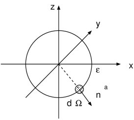
Fig. 5: We first compute the integral around the sphere as a simple example.

References

-
[1]
J. Maldacena,
Adv. Theor. Math. Phys. 2, (1998) 231
hep-th/9711200.
For a review, O. Aharony, S. S. Gubser, J. Maldacena, H. Ooguri and Y. Oz, Phys. Rept. 323, (2000) 183 hep-th/9905111. - [2] S. Rey and J. Yee, hep-th/9803001.
- [3] J. Maldacena, Phys. Rev. Lett. 80 (1998), 4859, hep-th/9803002.
- [4] D. Z. Freedman, S. D. Mathur, A. Matusis and L. Rastelli, Nucl. Phys. B 546 (1999), 96, hep-th/9804058.
- [5] N. Drukker, D. J. Gross and H. Ooguri, Phys. Rev. D 60 (1999), 125006, hep-th/9904191.
- [6] J. K. Erickson, G. W. Semenoff and K. Zarembo, Nucl. Phys. B 582, (2000), 155 hep-th/0003055.
- [7] N. Drukker and D. J. Gross, hep-th/0010274.