NEIP-01-004
hep-th/0106062
June 2001

We determine higher-derivative terms in the open superstring effective action with ${\rm U}(N)$ gauge group up to and including order $\alpha^{\prime 4}$ as can be extracted from 4 boson, 2 boson - 2 fermion and 4 fermion string scattering amplitudes. This yields corrections to the non-abelian Born-Infeld action involving higher derivatives as is relevant for studying D-branes beyond the slowly varying field approximation. While at order $\alpha^{\prime 2}$ the action has recently been shown to be a symmetrised trace, this no longer is true at order $\alpha^{\prime 3}$ or $\alpha^{\prime 4}$. We argue that these terms including higher derivatives are as important in a low-energy expansion as e.g. the much-discussed $\alpha^{\prime 4}F^{6}$ terms. In particular a computation of the fluctuation spectra at order $\alpha^{\prime 4}$ has to take into account these non-symmetrised trace higher-derivative terms computed here.

1 Introduction

The abelian Born-Infeld action [1] and its supersymmetric generalisation [2] capture the low-energy dynamics of open superstrings without Chan-Paton factors or, equivalently, of a single D9-brane. The analogous description in the presence of several D-branes is not known. For $N$ D$p$-branes the gauge group is ${\rm U}(N)$ and the $9-p$ embedding coordinates, on which all background fields depend, are ${\rm U}(N)$-valued matrices. To avoid this difficulty one can restrict oneself to studying D9-branes only. The leading low-energy limit of the effective action then is ${\rm U}(N)$ super Yang-Mills theory. There has been quite some controverse, however, concerning the higher-order corrections. It was proposed that they are again captured by some non-abelian generalisation of the Born-Infeld action with the trace over the ${\rm U}(N)$-generators being a symmetrised trace [3]. While this proposal assumed that derivatives of the Yang-Mills field strength are small in an appropriate sense and can be neglected, it allows for large fields with $\alpha^{\prime}F$ of order one. The symmetrised trace proposal was challenged at order $\alpha^{\prime 4}F^{6}$ by comparing fluctuation spectra of this non-abelian Born-Infeld action with background magnetic fields against a direct calculation of the spectrum from the dual picture of D-branes at angles [4, 5]. There were further indications from requiring $\kappa$-symmetry of the effective action that deviations from a symmetrised trace may already occur at order $\alpha^{\prime 2}$ for terms involving fermions [6].

The most direct way to settle this issue would be to obtain the effective action from open superstring scattering amplitudes. While this yielded the bosonic terms through order $\alpha^{\prime 2}F^{4}$ long ago [7], the full action at this order, including fermions, as deduced from the string scattering amplitudes was obtained recently [8]. At this order, the symmetrised trace turns out to be the correct answer, and moreover, it is uniquely determined from the scattering amplitudes (up to field redefinitions - as always). Independently it was shown [9] that imposing linear susy at order $\alpha^{\prime 2}$ (almost) uniquely leads to the same action. The conflict with $\kappa$-symmetry was resolved [8] by realising that $\kappa$-symmetry actually fails at orders higher than those considered in [6].

The expansion of the action can be viewed as an expansion in $\alpha^{\prime}$ and the Yang-Mills coupling $g$, with $\alpha^{\prime}gF_{\mu\nu}$ being dimensionless. Thus the lowest order $F^{2}$ term can be corrected by $\alpha^{\prime 2}g^{2}F^{4}$, $\alpha^{\prime 3}g^{3}F^{5}$, $\alpha^{\prime 4}g^{4}F^{6}$ etc, but also by terms of the form $\alpha^{\prime 3}g^{2}D^{2}F^{4}$ and $\alpha^{\prime 4}g^{2}D^{4}F^{4}$ etc. The standard assumption of large but slowly-varying fields is that one can neglect $\alpha^{\prime 3}g^{2}D^{2}F^{4}$ with respect to $\alpha^{\prime 3}g^{3}F^{5}$ etc. While it was always clear that there is some ambiguity here in the non-abelian case since $[D,D]\sim gF$, it was argued that the assumption would still be valid in a broad class of situations.

I will instead point out that allowing large fields one also has to allow large derivatives. There are two simple arguments, one formal and one physical. The formal argument is specific to the non-abelian case and was pointed out to me by Alex Sevrin: If one is interested in the equations of motion or in the fluctuation spectra rather than in the action itself, one has to vary once or twice with respect to $A_{\mu}$. Varying e.g. $\alpha^{\prime 4}g^{4}F^{6}$ twice yields a term of the form $\alpha^{\prime 4}g^{4}F^{2}(DF)^{2}$. On the other hand, the covariant derivatives $D_{\mu}$ also contains $gA_{\mu}$ and varying $\alpha^{\prime 4}g^{2}(DF)^{4}$ twice also leads to the same term $\alpha^{\prime 4}g^{4}F^{2}(DF)^{2}$. So there seems to be no reason to include only the $F^{6}$ term and not the $(DF)^{4}$ term.

The second argument applies to both the non-abelian and the abelian case. The basic idea is simple: if there is some region ${\cal R}$ in space where the fields are large, with $\alpha^{\prime}gF$ of order one, they also have to fall off to zero far from this region. If they fall off slowly enough to have small derivatives, then they actually stay large over a region much bigger than ${\cal R}$. The total energy then is such that this configuration forms a black hole, so that gravitational effects can no longer be neglected and it is certainly not enough to only consider the effective action for the gauge fields. To avoid this scenario, the fields would have to fall off quickly enough outside the region ${\cal R}$, leading to large gradients with terms like $\alpha^{\prime 4}g^{2}(DF)^{4}$ comparable to $\alpha^{\prime 4}g^{4}F^{6}$.

Let me make the latter argument a bit more quantitative. For simplicity, we make the argument in the more familiar setting of four dimensions and then indicate how it extends to arbitrary dimensions. We also drop all irrelevant numerical factors of order one.

The Schwarzschild radius $R_{H}$ of a mass $M$ object is $R_{H}\sim{M\over M_{P}^{2}}$ with $M_{p}$ being the Planck mass. We will assume that the string scale ${1\over\sqrt{\alpha^{\prime}}}$ is not very different from $M_{P}$ so that $R_{H}\sim\alpha^{\prime}M$. Consider a Yang-Mills field configuration with

$$\alpha^{\prime}F\sim\lambda\ ,$$ (1.1)

where $\lambda$ is a dimensionless parameter controlling the strength of the field. Suppose this configuration extends over some region and falls to zero within a radius $R$. The derivatives then are at least

$$\alpha^{\prime}DF\sim{\lambda\over R}$$ (1.2)

over part of this region. The total energy contained within this region is $M\sim F^{2}R^{3}\sim{\lambda^{2}R^{3}\over\alpha^{\prime 2}}$ with the Schwarzschild radius being $R_{H}\sim{\lambda^{2}R^{3}\over\alpha^{\prime}}$. This configuration will avoid being a black hole if $R>R_{H}$. i.e. $R\ {<\atop\sim}\ {\sqrt{\alpha^{\prime}}\over\lambda}$. But this implies that the derivatives are

$$\alpha^{\prime 3/2}DF\ \ {\textstyle{>\atop\sim}}\ \ \lambda^{2}$$ (1.3)

and cannot be neglected. Specifically, for various terms that appear in the action we get

$$\alpha^{\prime 4}F^{6}\sim{\lambda^{6}\over\alpha^{\prime 2}}\quad,\quad\alpha^{\prime 3}F^{2}(DF)^{2}\ \ {\textstyle{>\atop\sim}}\ \ {\lambda^{6}\over\alpha^{\prime 2}}\quad,\quad\alpha^{\prime 4}(DF)^{4}\ \ {\textstyle{>\atop\sim}}\ \ {\lambda^{8}\over\alpha^{\prime 2}}\ .$$ (1.4)

Choosing a small $\lambda$, one can make $\alpha^{\prime 4}(DF)^{4}$ smaller than $\alpha^{\prime 4}F^{6}$ by a factor $\lambda^{2}$. But small $\lambda$ means small fields, somewhat contrary to the assumptions. In any case, the higher-derivative term $\alpha^{\prime 3}F^{2}(DF)^{2}$ is exactly as important, if not more, as $\alpha^{\prime 4}F^{6}$, whatever the size of $\lambda$.

This argument can be extended to any space-time dimension $d$ where various powers of $d$ appear in various places, but the qualitative conclusion remains the same: To stay within the validity of the whole scheme, one should avoid that a black hole is formed. This necessarily implies that higher-derivative terms are as important as higher-order non-derivative terms.

With this motivation in mind, in this paper, I will determine higher-derivative corrections to the non-abelian Born-Infeld action, by working out these corrections to the open superstring effective action as it can be obtained from four-point scattering amplitudes. The four-point amplitudes are well-known and can be easily expanded in $\alpha^{\prime}$. It is then not too difficult to match these amplitudes against those obtained from an effective action including not more than four fields ($F_{\mu\nu}$ or fermions $\chi$, so the action is of order $g^{2}$ in the Yang-Mills coupling) but with an arbitrary number of derivatives. Thus we determine the complete action at order $\alpha^{\prime 3}g^{2}$ and at order $\alpha^{\prime 4}g^{2}$. As it is obvious from the expansion of the scattering amplitudes, the effective action at order $\alpha^{\prime 3}g^{2}$ is proportional the the product of two structure constants of the gauge group and hence is not a symmetrised trace. Also, at order $\alpha^{\prime 4}g^{2}$, there are two types of contributions, some again proportional the the product of two structure constants, and others being a symmetrised trace.

The plan of this paper is the following: in section 2, we present the various four-point string scattering amplitudes, with particular emphasis on the various combinations of the traces over the ${\rm U}(N)$ generators that appear, and give their expansions up to order $\alpha^{\prime 6}$. In section 3, we set up the computation of the effective action and briefly recall the results of [8] at order $\alpha^{\prime 2}$. In section 4 we compute the complete action including fermions at order $\alpha^{\prime 3}$ (and $\sim g^{2}$) while in section 5 we obtain the complete action at order $\alpha^{\prime 4}$ (and $\sim g^{2}$).

While the present paper was typed, a paper by Refolli, Santambrogio, Terzi and Zanon [10] appeared which also determines higher-derivative correction to the non-abelian Born-Infeld action. While the paper [10] only considers the bosonic part of the action and only with two derivatives, it also contains some information on $F^{5}$ terms.

2 Open superstring four-point scattering amplitudes

In this section we will first review the computation of the tree-level open string (disc) four-point amplitudes between the massless gauge bosons and their fermionic partners (gauginos) and then study in some detail their expansion in powers of $\alpha^{\prime}$. There is a 4 boson, a 4 fermion and a 2 boson / 2 fermion amplitude. We take the external momenta $k_{1},\ldots k_{4}$ all as incoming, assign Chan-Paton labels $a,b,c,d=1,\ldots{\rm dim\ U}(N)$, and wave-functions $u_{i}$ to the external fermions and polarisations $\epsilon_{j}$ to the external bosons. This is depicted in Fig. 1 for the example of a 2 boson / 2 fermion amplitude.

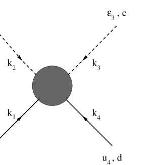
Figure 1: 2 boson / 2 fermion scattering amplitude

Any of these 4 point amplitudes is a sum of six disc diagrams corresponding to the 6 different cyclic orderings of the vertex operators as shown in Fig. 2.

Figure 2: The six different cyclic orderings

The contribution of each of the six orderings then is given [11, 12] by the product of

1.) a trace of the product of matrices $\lambda_{a}$ in the fundamental representation of ${\rm U}(N)$, taken in the cyclic order given by the diagram of Fig. 2, e.g. for the first one: $\,{\rm tr}\,\lambda_{a}\lambda_{b}\lambda_{c}\lambda_{d}\equiv t_{abcd}$

2.) a function $G$ depending on the two Mandelstam variables “flowing” through the diagram “horizontally” and “vertically”. For the first diagram of Fig. 2 e.g. the vertical momentum flow gives $(k_{1}+k_{2})^{2}=s$ while the horizontal momentum flow gives $(k_{1}+k_{4})^{2}=u$. Clearly, the 1. and 2. diagram give $G(s,u)$, the 3. and 4. give $G(s,t)$ and the 5. and 6. give $G(t,u)$. The function $G$ is given by

$$G(s,t)=\alpha^{\prime 2}{\Gamma(-\alpha^{\prime}s)\Gamma(-\alpha^{\prime}t)\over\Gamma(1-\alpha^{\prime}s-\alpha^{\prime}t)}$$ (2.1)

and is the same independent of the nature (boson or fermion) of the massless external states.

3.) a kinematic factor $K$ depending on the polarisations and wave-functions in the given cyclic order as well as on the momenta. It is independent of $\alpha^{\prime}$. This factor would actually be the same also for loop amplitudes. In the present example of 2 boson / 2 fermion scattering of Fig 1, the 3. diagram of Fig. 2 would e.g. come with a $K(u_{1},\epsilon_{2},u_{4},\epsilon_{3})$.

4.) a normalisation factor which we will take to be $-8ig^{2}$.

5.) a minus sign for any diagram in Fig. 2 which differs from the first one by the permutation of two fermions. Note that these signs will be cancelled in the end by the corresponding antisymmetry of the $K$-factor.

Let us now discuss these ingredients in more detail.

2.1 The traces

The traces come in 3 combinations (recall that $t_{abcd}\equiv\,{\rm tr}\,\lambda_{a}\lambda_{b}\lambda_{c}\lambda_{d}$):

$$T_{1}=t_{abcd}+t_{dcba}\quad,\quad T_{2}=t_{abdc}+t_{cdba}\quad,\quad T_{3}=t_{acbd}+t_{dbca}\ .$$ (2.2)

Using $[\lambda_{a},\lambda_{b}]=if_{abc}\lambda_{c}$ and $\{\lambda_{a},\lambda_{b}\}=d_{abc}\lambda_{c}$ as well as the normalisation $\,{\rm tr}\,\lambda_{a}\lambda_{b}=\delta_{ab}$ it is easy to show that

$$T_{1}+T_{2}+T_{3}=6\,{\rm str}\,\lambda_{a}\lambda_{b}\lambda_{c}\lambda_{d}={1\over 2}\left(d_{abe}d_{cde}+d_{ace}d_{bde}+d_{ade}d_{bce}\right)$$ (2.3)

$$T_{2}-T_{1}=f_{abe}f_{cde}\ ,\quad T_{2}-T_{3}=f_{ace}f_{bde}\ ,\quad T_{1}-T_{3}=f_{ade}f_{bce}\ .$$ (2.4)

Using the Jacobi identities of the appendix we also obtain

$$T_{1} = {1\over 2}\left(d_{abe}d_{cde}+d_{ade}d_{bce}-d_{ace}d_{bde}\right)$$ (2.5)

$$T_{2} = {1\over 2}\left(d_{abe}d_{cde}+d_{ace}d_{bde}-d_{ade}d_{bce}\right)$$ (2.6)

$$T_{3} = {1\over 2}\left(d_{ace}d_{bde}+d_{ade}d_{bce}-d_{abe}d_{cde}\right)\ .$$ (2.7)

2.2 The function $G$

The dependence of the amplitudes on the Mandelstam variables is contained in the function $G$ as given in eq. (2.1). Its expansion in powers of $\alpha^{\prime}$ is, up to and including $\alpha^{\prime 6}$ terms:

$$G(s,t) = {1\over st}-{\pi^{2}\over 6}\alpha^{\prime 2}+{c_{2}\over 2}(s+t)\alpha^{\prime 3}-{\pi^{4}\over 360}(4s^{2}+4t^{2}+st)\alpha^{\prime 4}$$ (2.8)

$$+ \left[{c_{4}\over 24}(s+t)(s^{2}+t^{2}+st)-{\pi^{2}c_{2}\over 12}(s+t)st\right]\alpha^{\prime 5}$$ (2.9)

$$+ \left[{c_{2}^{2}\over 8}(s+t)^{2}st-{\pi^{6}\over 15120}(16s^{4}+16t^{4}+12s^{3}t+12st^{3}+23s^{2}t^{2})\right]\alpha^{\prime 6}+{\cal O}(\alpha^{\prime 7})\ ,$$ (2.10)

where the $c_{n}$ are defined by

$$c_{n}={{\rm d}^{n}\psi(z)\over{\rm d}z^{n}}\Big{|}_{z=1}={{\rm d}^{n+1}\log\Gamma(z)\over{\rm d}z^{n+1}}\Big{|}_{z=1}\ ,$$ (2.11)

and in particular $c_{2}=2\zeta(3)\simeq-2.40411$ and $c_{4}\simeq-24.8863$.

Using $s+t=-u$ we may rewrite $G$ in a way which makes explicit the terms which are invariant when changing the arguments:

$$G(s,t) = {1\over st}-{\pi^{2}\over 6}\,\alpha^{\prime 2}-\zeta(3)u\,\alpha^{\prime 3}-\left[{\pi^{4}\over 180}(s^{2}+t^{2}+u^{2})-{\pi^{4}\over 120}st\right]\alpha^{\prime 4}$$ (2.12)

$$+ \left[{\pi^{2}\zeta(3)\over 6}stu-{c_{4}\over 48}(s^{2}+t^{2}+u^{2})u\right]\alpha^{\prime 5}$$ (2.13)

$$+ \Bigg{[}-{\pi^{6}\over 2880}(s^{2}+t^{2}+u^{2})^{2}+{\pi^{6}\over 3024}(s^{2}+t^{2}+u^{2})\left(st+{u^{2}\over 2}\right)$$ (2.15)

$$\quad+\left({\pi^{6}\over 3024}+{\zeta(3)^{2}\over 2}\right)(stu)\,u\Bigg{]}\alpha^{\prime 6}+{\cal O}(\alpha^{\prime 7})\ ,$$

2.3 The kinematical factors $K$

The $K$ factors are given in ref. [11]. Some care has to be exercised while copying the formula since our conventions are different from those of ref. [11].

For 4 boson we get:

$$K(\epsilon_{1},\epsilon_{2},\epsilon_{3},\epsilon_{4})=-{tu\over 4}\epsilon_{1}\cdot\epsilon_{2}\,\epsilon_{3}\cdot\epsilon_{4}-{su\over 4}\epsilon_{1}\cdot\epsilon_{3}\,\epsilon_{2}\cdot\epsilon_{4}-{st\over 4}\epsilon_{1}\cdot\epsilon_{4}\,\epsilon_{2}\cdot\epsilon_{3}-{s\over 2}{\cal K}_{s}-{t\over 2}{\cal K}_{t}-{u\over 2}{\cal K}_{u}$$ (2.16)

where

$${\cal K}_{s} = \epsilon_{1}\cdot k_{4}\,\epsilon_{3}\cdot k_{2}\,\epsilon_{2}\cdot\epsilon_{4}+\epsilon_{2}\cdot k_{3}\,\epsilon_{4}\cdot k_{1}\,\epsilon_{1}\cdot\epsilon_{3}+\epsilon_{1}\cdot k_{3}\,\epsilon_{4}\cdot k_{2}\,\epsilon_{2}\cdot\epsilon_{3}+\epsilon_{2}\cdot k_{4}\,\epsilon_{3}\cdot k_{1}\,\epsilon_{1}\cdot\epsilon_{4}$$ (2.17)

$${\cal K}_{t} = {\cal K}_{s}|_{2\leftrightarrow 3}$$ (2.18)

$${\cal K}_{u} = {\cal K}_{s}|_{2\leftrightarrow 4}$$ (2.19)

Note that $K(\epsilon_{1},\epsilon_{2},\epsilon_{3},\epsilon_{4})$ is completely symmetric under any permutation $i\leftrightarrow j$ and it vanishes if we replace $\epsilon_{i}$ by $k_{i}$ as required by gauge invariance.

For four fermions the K-factor is given by

$$K(u_{1},u_{2},u_{3},u_{4})={s\over 8}\,{\overline{u}}_{1}\gamma_{\mu}u_{4}\,{\overline{u}}_{2}\gamma^{\mu}u_{3}-{u\over 8}\,{\overline{u}}_{1}\gamma_{\mu}u_{2}\,{\overline{u}}_{4}\gamma^{\mu}u_{3}\ .$$ (2.20)

The $u_{i}$ are the (commuting) fermion ten-dimensional Majorana-Weyl wave-functions. Hence we have ${\overline{u}}_{i}\gamma^{\mu}u_{j}={\overline{u}}_{j}\gamma^{\mu}u_{i}$ and the Fierz identity

$${\overline{u}}_{1}\gamma_{\mu}u_{2}\,{\overline{u}}_{3}\gamma^{\mu}u_{4}+{\overline{u}}_{1}\gamma_{\mu}u_{3}\,{\overline{u}}_{4}\gamma^{\mu}u_{2}+{\overline{u}}_{1}\gamma_{\mu}u_{4}\,{\overline{u}}_{2}\gamma^{\mu}u_{3}=0$$ (2.21)

which together with the relation $s+t+u=0$ implies that $K(u_{1},u_{2},u_{3},u_{4})$ is completely antisymmetric under the exchange of any two fermions, e.g. we have $K(u_{1},u_{2},u_{4},u_{3})=-K(u_{1},u_{2},u_{3},u_{4})$ etc.

For two fermions and two bosons, ref. [11] considers two cases separately: the two fermions are adjacent or not. Both cases actually lead to the same $K$-factor as we now show. For fermions that are adjacent in the cyclic order we get from [11]

$$K(u_{1},\epsilon_{2},\epsilon_{3},u_{4})={u\over 8}A+{s\over 8}B$$ (2.22)

where we define the convenient expressions (${k\kern-5.0pt/}\equiv k_{\mu}\gamma^{\mu}$)

$$A = {\overline{u}}_{1}{\epsilon\kern-3.99994pt/}_{2}({k\kern-5.0pt/}_{3}+{k\kern-5.0pt/}_{4}){\epsilon\kern-3.99994pt/}_{3}u_{4}$$ (2.23)

$$B = 2{\overline{u}}_{1}\left({\epsilon\kern-3.99994pt/}_{3}\,k_{3}\cdot\epsilon_{2}-{\epsilon\kern-3.99994pt/}_{2}\,k_{2}\cdot\epsilon_{3}-{k\kern-5.0pt/}_{3}\,\epsilon_{2}\cdot\epsilon_{3}\right)u_{4}\ .$$ (2.24)

Using the on-shell properties

$$k_{2}\cdot\epsilon_{2}=k_{3}\cdot\epsilon_{3}={k\kern-5.0pt/}_{4}u_{4}={\overline{u}}_{1}{k\kern-5.0pt/}_{1}=0$$ (2.25)

one easily shows

$$A|_{2\leftrightarrow 3} = A-B\quad,\quad A|_{1\leftrightarrow 4}=B-A$$ (2.26)

$$B|_{2\leftrightarrow 3} = -B\quad\quad,\quad B|_{1\leftrightarrow 4}=B\ .$$ (2.27)

It then follows that $K(u_{1},\epsilon_{2},\epsilon_{3},u_{4})$ is symmetric under the exchange of the two bosons and antisymmetric under exchange of the two fermions. If the fermions are not adjacent in the cyclic ordering we get instead from [11]

$$K(u_{1},\epsilon_{2},u_{4},\epsilon_{3}) = -{t\over 8}\,{\overline{u}}_{1}{\epsilon\kern-3.99994pt/}_{2}({k\kern-5.0pt/}_{3}+{k\kern-5.0pt/}_{4}){\epsilon\kern-3.99994pt/}_{3}u_{4}-{s\over 8}\,{\overline{u}}_{1}{\epsilon\kern-3.99994pt/}_{3}({k\kern-5.0pt/}_{2}+{k\kern-5.0pt/}_{3}){\epsilon\kern-3.99994pt/}_{2}u_{4}$$ (2.28)

$$= -{t\over 8}A-{s\over 8}(A-B)={u\over 8}A+{s\over 8}B$$ (2.29)

which is actually identical to the other $K$-factor (2.22) for adjacent fermions. Thus there is a single $K$-factor for 2 bosons / 2 fermions, just as for 4 boson or 4 fermion scattering.

These kinematical factors are actually determined by the required (anti)symmetry, (linearized) gauge invariance and dimensional reasoning. In the 2 fermion / 2 boson case e.g. the (anti)symmetry and dimensional reasoning require $K$ to be of the form $K_{\beta}={u\over 8}A+{1\over 8}\left(s+\beta\left(t-{u\over 2}\right)\right)B$ and then gauge invariance (vanishing upon $\epsilon_{i}\to k_{i}$) fixes $\beta=0$.

It follows that any of the four-point (tree-level) amplitudes we are interested in takes the form

$$A_{4} = -8ig^{2}\ K(1,2,3,4)\ \times$$ (2.30)

$$\times \left\{(t_{abcd}+t_{dcba})G(s,u)+(t_{abdc}+t_{cdba})G(s,t)+(t_{acbd}+t_{dbca})G(t,u)\right\}\ .$$ (2.31)

Note that any minus signs introduced when two fermions in Fig. 2 are permuted with respect to the reference configuration has been cancelled by another minus sign when performing the same permutation on the arguments of $K$ to rewrite it as $K(1,2,3,4)$.

2.4 $\alpha^{\prime}$-expansion of the four-point amplitude

Inserting the $\alpha^{\prime}$-expansion of the $G$-function into (2.30) we get for any of the four-point amplitudes

$$A_{4}=-8ig^{2}\ K(1,2,3,4)\sum_{N=0}^{\infty}a_{4}^{(n)}\alpha^{\prime n}\ .$$ (2.33)

The lowest order term can be written in 3 equivalent ways:

$$a_{4}^{(0)} = {1\over s}\left({1\over t}f_{ace}f_{bde}+{1\over u}f_{ade}f_{bce}\right)$$ (2.34)

$$= -{1\over u}\left({1\over s}f_{abe}f_{cde}+{1\over t}f_{ace}f_{bde}\right)$$ (2.35)

$$= {1\over t}\left({1\over s}f_{abe}f_{cde}-{1\over u}f_{ade}f_{bce}\right)\ .$$ (2.36)

This vanishes in the abelian case: there is no lowest order photon-photon scattering. Clearly, there is no order $\alpha^{\prime}$ contribution and $a_{4}^{(1)}=0$.

The obvious fact about the order $\alpha^{\prime 2}$ contribution is that it is always a symmetrised trace. Indeed, at order $\alpha^{\prime 2}$ the function $G$ is just a constant, and thus all traces contribute equally, leading to a symmetrised trace:

$$a_{4}^{(2)}=-\pi^{2}\,{\rm str}\,\lambda_{a}\lambda_{b}\lambda_{c}\lambda_{d}\ .$$ (2.37)

At order $\alpha^{\prime 3}$, since $s+t+u=0$, no symmetrised trace part remains and the contribution only contains products of structure constants $f$ (as was also the case at order $\alpha^{\prime 0}$ for the same reason):

$$a_{4}^{(3)} = \zeta(3)\left(tf_{abe}f_{cde}+sf_{ace}f_{bde}\right)$$ (2.38)

$$= {\zeta(3)\over 3}\left[(t-u)f_{abe}f_{cde}+(s-u)f_{ace}f_{bde}+(s-t)f_{ade}f_{bce}\right]$$ (2.39)

which again can be rewritten in various ways.

The order $\alpha^{\prime 4}$ contribution is more interesting as it contains a manifestly symmetric and a non-symmetric piece:

$$a_{4}^{(4)} = -{\pi^{4}\over 24}(s^{2}+t^{2}+u^{2})\,{\rm str}\,\lambda_{a}\lambda_{b}\lambda_{c}\lambda_{d}$$ (2.40)

$$+ {\pi^{4}\over 360}\left[s(t-u)f_{abe}f_{cde}+t(s-u)f_{ace}f_{bde}+u(s-t)f_{ade}f_{bce}\right]\ .$$ (2.41)

Similarly at order $\alpha^{\prime 5}$:

$$a_{4}^{(5)} = \pi^{2}\zeta(3)\ stu\,\,{\rm str}\,\lambda_{a}\lambda_{b}\lambda_{c}\lambda_{d}$$ (2.42)

$$+ {c_{4}\over 48}(s^{2}+t^{2}+u^{2})\left(tf_{abe}f_{cde}+sf_{ace}f_{bde}\right)\ .$$ (2.43)

Finally, we give the order $\alpha^{\prime 6}$ contribution to the four-point amplitudes:

$$a_{4}^{(6)} = -{\pi^{6}\over 480}(s^{2}+t^{2}+u^{2})^{2}\,{\rm str}\,\lambda_{a}\lambda_{b}\lambda_{c}\lambda_{d}$$ (2.44)

$$+ {\pi^{6}\over 6048}(s^{2}+t^{2}+u^{2})\left[s(t-u)f_{abe}f_{cde}+t(s-u)f_{ace}f_{bde}+u(s-t)f_{ade}f_{bce}\right]$$ (2.45)

$$- \left({\pi^{6}\over 3024}+{\zeta(3)^{2}\over 2}\right)stu\left[tf_{abe}f_{cde}+sf_{ace}f_{bde}\right]\ .$$ (2.46)

Note that, by construction, all $a_{4}^{(n)}$ are completely symmetric under exchange of any two external states, so that the symmetry properties of the amplitude are correctly given by those of the kinematical factors $K(1,2,3,4)$.

The explicit forms of the various four-point amplitudes up to and including the order $\alpha^{\prime 2}$ terms are given in [8].

3 The effective action at order $\alpha^{\prime 2}$

In this section we set up the computation of the effective action. Since the determination of the $\alpha^{\prime 3}$ and $\alpha^{\prime 4}$ terms in the next two sections is an extension of the $\alpha^{\prime 2}$ computation, it is most useful to first quickly review the latter as obtained in [8] by matching the amplitudes computed from the effective action against the string amplitudes at order $\alpha^{\prime 2}$. This is the purpose of the present section.

3.1 The $\alpha^{\prime}$ expansion

Our goal is to find the effective action which reproduces the $\alpha^{\prime}$-expansion of the open superstring four-point amplitude of the previous section. Note that this determines the action only up to on-shell terms $\sim\gamma^{\mu}\partial_{\mu}\chi$ or $\sim\partial_{\mu}F^{\mu\nu}$. At lowest order in $\alpha^{\prime}$ this is of course well-known to be the ${\rm U}(N)$ ${\cal N}=1$ super Yang-Mills theory in ten dimensions

$${\cal L}_{\rm SYM}=\,{\rm tr}\,\left(-{1\over 4}F_{\mu\nu}F^{\mu\nu}+{i\over 2}{\overline{\chi}}\gamma^{\mu}D_{\mu}\chi\right).$$ (3.1)

The order $\alpha^{\prime 0}$ amplitudes serve to fix the normalisations correctly. Our Feynman rules and other conventions are given in the appendix. At higher orders in $\alpha^{\prime}$, the possible terms are given by dimensional analysis: in any space-time dimension $d$, the combination $gA_{\mu}$ of the YM coupling constant and the gauge field has canonical dimension one, and thus $gF_{\mu\nu}$ has dimension two. Similarly, the analogous combination for the fermion $g\chi$ has canonical dimension ${3\over 2}$. Thus dimensionless quantities are $\alpha^{\prime}gF_{\mu\nu}$ and $\alpha^{\prime 2}g^{2}\,{\overline{\chi}}\gamma D\chi$ This leads to the following possible terms beyond ${\cal L}_{\rm SYM}$.

At order $\alpha^{\prime}$ there is only $\alpha^{\prime}g\,{\overline{\chi}}\gamma D\chi F$ while at order $\alpha^{\prime 2}$ we have $(\alpha^{\prime}g)^{2}\,FFFF$, $(\alpha^{\prime}g)^{2}\,{\overline{\chi}}\gamma D\chi FF$ and $(\alpha^{\prime}g)^{2}\,{\overline{\chi}}\gamma D\chi\,{\overline{\chi}}\gamma D\chi$ with various Lorentz and Lie algebra structures. One could also replace in some terms $gF$ by two covariant derivatives leading e.g. to $\alpha^{\prime 2}g{\overline{\chi}}\gamma_{\mu}D^{\rho}D_{\nu}D_{\rho}\chi F^{\mu\nu}$ or $\alpha^{\prime 2}g{\overline{\chi}}\gamma^{\rho}D_{\mu}D_{\rho}D_{\nu}\chi F^{\mu\nu}$ etc. Upon commuting two derivatives (which gives back $gF$) this contains either $D^{2}\chi$ or ${D\kern-6.00006pt/}\chi$ which both vanish on-shell. Similarly, any term of the form $\alpha^{\prime 2}gFDFDF$ either vanishes on-shell ($\sim D_{\rho}F^{\mu\rho}$), possibly after partial integration, or gives back some $(\alpha^{\prime}g)^{2}FFFF$ term. Thus there are no “higher-derivative” terms at order $\alpha^{\prime 2}$.

Note that all our order $\alpha^{\prime 2}$ terms contain at least four fields ($\chi$ or $A_{\mu}$) and hence each contribute to the four-point amplitude only via a single vertex diagram (1PI) while the order $\alpha^{\prime}$ terms contain 3, 4 or 5 fields and contribute to the four-point amplitude both a 1PI piece and via one-particle reducible $s$, $t$ and $u$-channel diagrams. All these terms would also contribute to higher-than-four-point, say six-point, amplitudes, both via one-particle reducible and irreducible diagrams.

At order $\alpha^{\prime 3}$ we encounter $(\alpha^{\prime}g)^{3}F^{5}$, but also $\alpha^{\prime 3}g^{2}F^{2}(DF)^{2}$ (which now does not vanish on-shell). Similarly at order $\alpha^{\prime 4}$ we have e.g. $(\alpha^{\prime}g)^{4}F^{6}$ and $\alpha^{\prime 4}g^{2}F^{2}(D^{2}F)^{2}$. While the former terms cannot contribute to the four-point amplitude, the latter do. Comparing these contributions with the corresponding $\alpha^{\prime}$-expansion of the string amplitude in sections 4 and 5, we will determine these higher order terms with no more than a total of four field strengths $F$ or fermion fields $\chi$.

A remark is in order about on-shell terms. Consider e.g. ${\tilde{\alpha}}^{\prime 2}({\overline{\chi}}{\partial\kern-5.0pt/}\chi)^{2}$ or ${\tilde{\alpha}}^{\prime 2}{\overline{\chi}}{\partial\kern-5.0pt/}\chi F_{\rho\sigma}F^{\rho\sigma}$. They vanish on-shell and do not contribute to the four-point amplitude. These terms only contribute to the four-point amplitude via a single vertex (1PI diagram) and the fields involved are necessarily all on-shell. However, if we would compute the six-point amplitude at order $\alpha^{\prime 4}$ using two such vertices joined by one fermion propagator in a one particle reducible diagram, the fermion might well be off-shell and such a term could not be dropped. This is consistent with the following interpretation of on-shell terms: an order $\alpha^{\prime 2}$ on-shell term can be removed by a field redefinition involving an order $\alpha^{\prime 2}$ piece. But when substituting the new fields in the order $\alpha^{\prime 2}$ interaction, this will also generate a new interaction at order $\alpha^{\prime 4}$ that will contribute irreducibly to the six-point amplitude.

3.2 The ansatz for the non-abelian effective action

We write the effective action up to and including order $\alpha^{\prime 2}$ as

$${\cal L}={\cal L}_{\rm SYM}+{\cal L}_{\rm 4b}+{\cal L}_{\rm 2b/2f}+{\cal L}_{\rm 4f}+{\cal L}_{*}+{\cal O}(\alpha^{\prime 3})$$ (3.2)

with ${\cal L}_{\rm 4b}$, ${\cal L}_{\rm 2b/2f}$ and ${\cal L}_{\rm 4f}$ containing the order $\alpha^{\prime 2}$ terms needed to reproduce the string amplitudes to this order. The piece ${\cal L}_{*}$ contains any terms $\sim{\tilde{\alpha}}^{\prime 2}{D\kern-6.00006pt/}\chi$, $\sim{\tilde{\alpha}}^{\prime 2}D_{\mu}{\overline{\chi}}\gamma^{\mu}$, $\sim{\tilde{\alpha}}^{\prime 2}D_{\mu}F^{\mu\nu}$ that vanish on-shell and do not contribute to the four-point amplitudes as discussed above. In the following we write ${\cal L}_{1}\simeq{\cal L}_{2}$ if ${\cal L}_{1}$ and ${\cal L}_{2}$ only differ up to terms in ${\cal L}_{*}$ and up to partial integration.

The purely bosonic piece ${\cal L}_{\rm 4b}$ is well-known since long [7]:

$${\cal L}_{\rm 4b}={\tilde{\alpha}}^{\prime 2}\,{\rm str}\,\left({1\over 8}F_{\mu\nu}F^{\nu\rho}F_{\rho\sigma}F^{\sigma\mu}-{1\over 32}\left(F_{\mu\nu}F^{\mu\nu}\right)^{2}\right)$$ (3.3)

where

$${\tilde{\alpha}}^{\prime}=2\pi g\alpha^{\prime}\ .$$ (3.4)

Since this contains exactly four $F$’s the contribution to the four gluon amplitude is obtained by extracting the interaction where each $F^{a}_{\mu\nu}$ is replaced simply by $\partial_{\mu}A_{\nu}^{a}-\partial_{\nu}A_{\mu}^{a}$. There is then a single order $\alpha^{\prime 2}$ four gluon vertex contributing to the amplitude, and it is a straightforward exercise to show that the result coincides with the order $\alpha^{\prime 2}$ part of the string amplitude $A_{4}^{\rm 4b}$. In fact, it is not necessary to check all the terms in $K(\epsilon_{1},\epsilon_{2},\epsilon_{3},\epsilon_{4})$ since the structure of $K$ is fixed by gauge invariance and permutation symmetry. It is e.g. enough to check that (3.3) yields the $\epsilon_{1}\cdot\epsilon_{2}\,\epsilon_{3}\cdot\epsilon_{4}$ term with the correct coefficient. It is also easy to check that (3.3) is the unique interaction that reproduces the string four-gluon amplitude at order $\alpha^{\prime 2}$.

The other terms in (3.2) were determined in [8]. A possible order $\alpha^{\prime}$ term $ic_{1}d_{abc}{\overline{\chi}}^{a}\gamma_{\mu}D_{\nu}\chi^{b}F^{c\mu\nu}$ is first removed by a field redefinition $\chi^{a}\to\chi^{a}+{1\over 2}c_{1}\alpha^{\prime}d_{abc}F^{b}_{\rho\sigma}\gamma_{\rho\sigma}\chi^{c}$. Then a general ansatz for the mixed piece is

$${\cal L^{\prime}}_{\rm 2b/2f} = i{\tilde{\alpha}}^{\prime 2}y_{abcd}{\overline{\chi}}^{a}\gamma_{\mu}D_{\nu}\chi^{b}F^{c\mu\rho}F^{d\ \ \nu}_{\ \rho}+i{\tilde{\alpha}}^{\prime 2}z_{abcd}{\overline{\chi}}^{a}\gamma_{\mu}\gamma_{\nu}\gamma_{\rho}D_{\sigma}\chi^{b}F^{c\mu\nu}F^{d\rho\sigma}$$ (3.5)

$$= i{\tilde{\alpha}}^{\prime 2}{\widetilde{y}}_{abcd}{\overline{\chi}}^{a}\gamma_{\mu}D_{\nu}\chi^{b}F^{c\mu\rho}F^{d\ \ \nu}_{\ \rho}+i{\tilde{\alpha}}^{\prime 2}z_{abcd}{\overline{\chi}}^{a}\gamma_{\mu\nu\rho}D_{\sigma}\chi^{b}F^{c\mu\nu}F^{d\rho\sigma}$$ (3.6)

with

$${\widetilde{y}}_{abcd}=y_{abcd}+2z_{abcd}$$ (3.7)

and where the prime on ${\cal L}$ is just to remind us that this is the form after the field redefinition.

For the four fermion interaction ${\cal L}_{\rm 4f}$ a general ansatz is

$${\cal L}_{\rm 4f}={\tilde{\alpha}}^{\prime 2}g_{abcd}{\overline{\chi}}^{a}\gamma^{\mu}D^{\nu}\chi^{b}\,{\overline{\chi}}^{c}\gamma_{\mu}D_{\nu}\chi^{d}+{\tilde{\alpha}}^{\prime 2}h_{abcd}{\overline{\chi}}^{a}\gamma^{\mu}D^{\nu}\chi^{b}\,{\overline{\chi}}^{c}\gamma_{\nu}D_{\mu}\chi^{d}\ ,$$ (3.8)

since other terms like ${\tilde{\alpha}}^{\prime 2}j_{abcd}{\overline{\chi}}^{a}\gamma^{\mu\nu\rho}D_{\rho}\chi^{b}\,{\overline{\chi}}^{c}\gamma_{\mu}D_{\nu}\chi^{d}$ or ${\tilde{\alpha}}^{\prime 2}l_{abcd}{\overline{\chi}}^{a}\gamma^{\mu\nu\rho}D^{\sigma}\chi^{b}\,{\overline{\chi}}^{c}\gamma_{\mu\nu\rho}D_{\sigma}\chi^{d}$ can be rewritten, using Fierz identities, as a combination of the two terms in (3.8), up to terms $\sim{D\kern-6.00006pt/}\chi$ which do not contribute to the amplitude. Upon partial integration and dropping any terms that vanish on-shell, one sees that one may just as well assume that $h_{abcd}$ is symmetric under interchange of $a$ and $b$ or of $c$ and $d$. Similarly, we may assume

$$g_{abcd}=g_{cdab}\quad{\rm and}\quad g_{(ab)[cd]}=g_{[ab](cd)}=0\quad\Rightarrow\quad g_{abcd}=g_{badc}\ .$$ (3.9)

3.3 Matching the 2 boson / 2 fermion amplitude

The most convenient form of the relevant interaction is the first line of (3.5). It only contributes two terms to the 2 boson / 2 fermion interaction, obtained upon replacing $D_{\lambda}\to\partial_{\lambda}$ and $F^{a}_{\mu\nu}\to\partial_{\mu}A^{a}_{\nu}-\partial_{\nu}A^{a}_{\mu}$. Obviously, there is no order $\alpha^{\prime}$ piece, while the computation of the order $\alpha^{\prime 2}$ contribution to the amplitude is a bit lengthy but straightforward. It yields [8]

$$A_{4}^{\rm 2b/2f} = i{\tilde{\alpha}}^{\prime 2}\Bigg{\{}A(tz^{+}+sz^{-})$$ (3.16)

$$\phantom{i{\tilde{\alpha}}^{\prime 2}}+{\overline{u}}_{1}{\epsilon\kern-3.99994pt/}_{3}u_{4}\left[2k_{1}\cdot\epsilon_{2}(tz^{+}+sz^{-})+{1\over 2}(tk_{1}\cdot\epsilon_{2}-sk_{4}\cdot\epsilon_{2})(y_{dacb}+y_{adcb})\right]$$

$$\phantom{i{\tilde{\alpha}}^{\prime 2}}-{\overline{u}}_{1}{\epsilon\kern-3.99994pt/}_{2}u_{4}\left[2k_{4}\cdot\epsilon_{3}(tz^{+}+sz^{-})+{1\over 2}(tk_{4}\cdot\epsilon_{3}-sk_{1}\cdot\epsilon_{3})(y_{dabc}+y_{adbc})\right]$$

$$\phantom{i{\tilde{\alpha}}^{\prime 2}}-{\overline{u}}_{1}{k\kern-5.0pt/}_{3}u_{4}\epsilon_{2}\cdot\epsilon_{3}\left[-2tz^{+}+{s\over 2}(y_{adbc}+y_{dacb})-{t\over 2}(y_{dabc}+y_{adcb})\right]$$

$$\phantom{i{\tilde{\alpha}}^{\prime 2}}+{\overline{u}}_{1}{k\kern-5.0pt/}_{3}u_{4}\Big{[}k_{1}\cdot\epsilon_{2}k_{1}\cdot\epsilon_{3}(y_{dabc}-y_{dacb})+k_{4}\cdot\epsilon_{2}k_{4}\cdot\epsilon_{3}(y_{adcb}-y_{adbc})$$

$$\phantom{i{\tilde{\alpha}}^{\prime 2}+{\overline{u}}_{1}{k\kern-5.0pt/}_{3}u_{4}}-k_{1}\cdot\epsilon_{2}k_{4}\cdot\epsilon_{3}(4z^{-}+y_{adbc}+y_{dacb})$$

$$\phantom{i{\tilde{\alpha}}^{\prime 2}+{\overline{u}}_{1}{k\kern-5.0pt/}_{3}u_{4}}+k_{4}\cdot\epsilon_{2}k_{1}\cdot\epsilon_{3}(4z^{+}+y_{dabc}+y_{adcb})\Big{]}\Bigg{\}}$$

with

$$z^{+}=z_{dabc}+z_{adcb}\quad,\quad z^{-}=z_{adbc}+z_{dacb}$$ (3.17)

and where $A$ (and $B$) where defined in (2.23). Note that this vanishes if we replace $\epsilon_{i}\to k_{i}$, as required by gauge invariance.

Matching the result (3.16) to the corresponding string amplitude (recall that ${\tilde{\alpha}}^{\prime}=2\pi g\alpha^{\prime}$) yielded the following conditions [8]

$$z^{+}=z^{-}=-{1\over 4}\,{\rm str}\,\lambda_{a}\lambda_{b}\lambda_{c}\lambda_{d}\quad,\quad y_{adbc}+y_{dabc}=\,{\rm str}\,\lambda_{a}\lambda_{b}\lambda_{c}\lambda_{d}\quad,\quad y_{adbc}=y_{adcb}\ .$$ (3.18)

This can be equivalently written as

$$z_{abcd}+z_{badc}=-{1\over 4}\,{\rm str}\,\lambda_{a}\lambda_{b}\lambda_{c}\lambda_{d}\quad,\quad y_{(ab)cd}={1\over 2}\,{\rm str}\,\lambda_{a}\lambda_{b}\lambda_{c}\lambda_{d}\quad,\quad y_{ab[cd]}=0\ .$$ (3.19)

It was shown in [8] that, up to terms that secretly vanish on shell and hence can be eliminated by field redefinitions, the unique solution is

$$y_{abcd} = {1\over 2}\,{\rm str}\,\lambda_{a}\lambda_{b}\lambda_{c}\lambda_{d}$$ (3.20)

$$z_{abcd} = -{1\over 8}\,{\rm str}\,\lambda_{a}\lambda_{b}\lambda_{c}\lambda_{d}$$ (3.21)

3.4 Matching the 4 fermion amplitude

We will now review the contribution of ${\cal L}_{\rm 4f}$ to the 4 fermion amplitude. It was shown in [8] that the second term in ${\cal L}_{\rm 4f}$ cannot reproduce anything that looks like the string amplitude unless it can be transformed - using some Fierz identity - into a term with the same Lorentz index structure as the first one in ${\cal L}_{\rm 4f}$. This is only possible if $h_{abcd}$ is completely symmetric in all its indices. We begin by examining the contribution of the first term alone. Obviously, its contribution to the amplitude contains ${\overline{u}}_{1}\gamma_{\mu}u_{2}{\overline{u}}_{3}\gamma^{\mu}u_{4}$, ${\overline{u}}_{1}\gamma_{\mu}u_{4}{\overline{u}}_{2}\gamma^{\mu}u_{3}$ and ${\overline{u}}_{1}\gamma_{\mu}u_{3}{\overline{u}}_{2}\gamma^{\mu}u_{4}$. Using the Fierz identity (2.21) this last expression can be rewritten as a combination of the two other, and, upon taking into account (3.9) one gets [8]

$$A_{4}^{\rm 4f}|_{g-{\rm terms}} = -2i{\tilde{\alpha}}^{\prime 2}\Bigg{\{}\left[(g_{acbd}+g_{adbc})\,s-g_{adcb}\,t-g_{acdb}\,u\right]{\overline{u}}_{1}\gamma_{\mu}u_{4}{\overline{u}}_{2}\gamma^{\mu}u_{3}$$ (3.23)

$$\phantom{-2i{\tilde{\alpha}}^{\prime 2}\Bigg{\{}}-\left[(g_{acdb}+g_{abdc})\,u-g_{abcd}\,t-g_{acbd}\,s\right]{\overline{u}}_{1}\gamma_{\mu}u_{2}{\overline{u}}_{3}\gamma^{\mu}u_{4}\Bigg{\}}\ .$$

Comparing with the string amplitude one sees that, if and only if

$$g_{abcd}=g_{acbd}\ ,$$ (3.24)

the amplitude reduces to the desired form

$$A_{4}^{\rm 4f}|_{g-{\rm terms}}=-2i{\tilde{\alpha}}^{\prime 2}\left(g_{acbd}+g_{abdc}+g_{adcb}\right)\left(s\ {\overline{u}}_{1}\gamma_{\mu}u_{4}{\overline{u}}_{2}\gamma^{\mu}u_{3}-u\ {\overline{u}}_{1}\gamma_{\mu}u_{2}{\overline{u}}_{3}\gamma^{\mu}u_{4}\right)\ .$$ (3.25)

The condition (3.24) together with (3.9) and the results of the appendix on 4-index tensors determine $g_{abcd}$ to be of the form (dropping a piece that leads to a term that secretly vanishes on-shell)

$$g_{abcd}=g\,{\rm str}\,\lambda_{a}\lambda_{b}\lambda_{c}\lambda_{d}$$ (3.26)

Concerning the second term it was shown [8] that one needs

$$h_{abcd}=h\,{\rm str}\,\lambda_{a}\lambda_{b}\lambda_{c}\lambda_{d}$$ (3.27)

so that one has using Fierz identities

$$h_{abcd}{\overline{\chi}}^{a}\gamma_{\mu}D_{\nu}\chi^{b}\ {\overline{\chi}}^{c}\gamma^{\nu}D^{\mu}\chi^{d}\simeq{2\over 3}h_{abcd}{\overline{\chi}}^{a}\gamma_{\mu}D_{\nu}\chi^{b}\ {\overline{\chi}}^{c}\gamma^{\mu}D^{\nu}\chi^{d}={2\over 3}h\,{\rm str}\,{\overline{\chi}}\gamma_{\mu}D_{\nu}\chi\ {\overline{\chi}}\gamma^{\mu}D^{\nu}\chi\ ,$$ (3.28)

and the $h$-term contributes to the amplitude ${2\over 3}$ of the $g$-term. Matching to the string amplitude then requires $3g+2h=-{1\over 8}$. While the expansion of the Born-Infeld determinant leads to $g={1\over 8}$ and $h=-{1\over 4}$, one should keep in mind that the $g$-term and the $h$-term are really indistinguishable on-shell (modulo the factor ${2\over 3}$), i.e. up to field redefinitions.

3.5 The string effective action

The full effective action up to and including all order $\alpha^{\prime 2}\,g^{2}$ terms, bosonic, fermionic and mixed, can be written as [8]

$${\cal L}_{\rm string} = \,{\rm str}\,\Bigg{(}-{1\over 4}F_{\mu\nu}F^{\mu\nu}+{i\over 2}{\overline{\chi}}\gamma^{\mu}D_{\mu}\chi+{{\tilde{\alpha}}^{\prime 2}\over 8}F_{\mu\nu}F^{\nu\rho}F_{\rho\sigma}F^{\sigma\mu}-{{\tilde{\alpha}}^{\prime 2}\over 32}\left(F_{\mu\nu}F^{\mu\nu}\right)^{2}$$ (3.31)

$$\phantom{\,{\rm str}\,\Bigg{(}}+i{{\tilde{\alpha}}^{\prime 2}\over 4}{\overline{\chi}}\gamma_{\mu}D_{\nu}\chi F^{\mu\rho}F_{\rho}^{\ \nu}-i{{\tilde{\alpha}}^{\prime 2}\over 8}{\overline{\chi}}\gamma_{\mu\nu\rho}D_{\sigma}\chi F^{\mu\nu}F^{\rho\sigma}$$

$$\phantom{\,{\rm str}\,\Bigg{(}}+{{\tilde{\alpha}}^{\prime 2}\over 8}{\overline{\chi}}\gamma^{\mu}D^{\nu}\chi\,{\overline{\chi}}\gamma_{\mu}D_{\nu}\chi-{{\tilde{\alpha}}^{\prime 2}\over 4}{\overline{\chi}}\gamma^{\mu}D^{\nu}\chi\,{\overline{\chi}}\gamma_{\nu}D_{\mu}\chi\Bigg{)}+{\cal O}({\tilde{\alpha}}^{\prime 3}\,g^{2}\,,\alpha^{\prime 2}\,g^{3})\ .$$

As noted in [8], this coincides with the result of the following manipulation: Take the abelian Born-Infeld action and expand it up to and including order $\alpha^{\prime 2}$. Make the field redefinition to eliminate the order $\alpha^{\prime}$ term, and drop all “on-shell” terms $\sim{\tilde{\alpha}}^{\prime 2}{\partial\kern-5.0pt/}\chi$. Only then proceed to the obvious non-abelian generalisation and take a symmetrised trace.

4 The effective action at order $\alpha^{\prime 3}$

We can now go on and compare results for the amplitudes beyond order $\alpha^{\prime 2}$. For the string amplitudes the $\alpha^{\prime}$ expansion was easy to obtain and is given in section 2. As already discussed, these four-point amplitudes only allow us to obtain information on the field theory side on terms that are quartic (or less) in the fields. For example, at order $\alpha^{\prime 3}$ we can get information about terms like $\alpha^{\prime 3}g^{2}F^{2}(DF)^{2}$ but not $\alpha^{\prime 3}g^{3}F^{5}$. Thus we cannot go beyond order $g^{2}$ terms.

We begin with the action (3.31). There are cubic and quartic vertices of order $\alpha^{\prime 0}$ and quartic and higher vertices of order $\alpha^{\prime 2}$. As a consequence there cannot be any contribution to the four-point amplitudes at order $\alpha^{\prime 3}$ from one-particle reducible diagrams with vertices made from the interactions already contained in (3.31). All order $\alpha^{\prime 3}$ contributions to the four-point amplitudes come from new quartic (and higher) interactions of order $\alpha^{\prime 3}$. This same discussion then repeats itself at order $\alpha^{\prime 4}$ and so on. This is a considerable simplification since disentangling one-particle reducible from one-particle irreducible contributions in general is a rather cumbersome task.

From eqs. (2.33) and (2.38) we know that the four-point string amplitudes at order $\alpha^{\prime 3}$ are

$$A_{4}|^{\rm string}_{\alpha^{\prime 3}} = -8ig^{2}\alpha^{\prime 3}\ \zeta(3)\ \left(tf_{abe}f_{cde}+sf_{ace}f_{bde}\right)K(1,2,3,4)$$ (4.1)

$$= +8ig^{2}\alpha^{\prime 3}\ \zeta(3)\ \left(tf_{ade}f_{bce}+uf_{ace}f_{bde}\right)K(1,2,3,4)\ .$$ (4.2)

4.1 Four fermion terms

Lets first look at the four fermion interaction which we parametrize in a similar way as before:

$${\cal L}_{\rm 4f}^{\alpha^{\prime 3}}={\tilde{c}}g^{2}\alpha^{\prime 3}{\tilde{g}}_{abcd}\ {\overline{\chi}}^{a}\gamma^{\mu}D^{(\nu}D^{\rho)}\chi^{b}\ {\overline{\chi}}^{c}\gamma_{\mu}D_{(\nu}D_{\rho)}\chi^{d}$$ (4.3)

with ${\tilde{g}}_{abcd}={\tilde{g}}_{cdab}$. We wrote $D_{(\nu}D_{\rho)}$ since the antisymmetric piece is $D_{[\nu}D_{\rho]}\sim gF_{\nu\rho}$ and corresponds to an order $g^{3}$ term which would show up in a five-point amplitude. Said differently, for our purpose of computing four-point amplitudes we can replace $D_{\nu}D_{\rho}\to\partial_{\nu}\partial_{\rho}$ which is symmetric in $\nu$ and $\rho$. The computation of the amplitude then is very similar to the order $\alpha^{\prime 2}$ computation above in (3.23) except that we have more derivatives in the interaction, and a priori, ${\tilde{g}}$ has less symmetries. The result is

$$A_{4}^{\rm 4f}|_{\alpha^{\prime 3}} = {i\over 2}{\tilde{c}}g^{2}\alpha^{\prime 3}\Bigg{\{}\Big{[}({\tilde{g}}_{abcd}+{\tilde{g}}_{badc})t^{2}+({\tilde{g}}_{acbd}+{\tilde{g}}_{cadb})s^{2}$$ (4.7)

$$\phantom{-2i{\tilde{c}}g^{2}{\tilde{\alpha}}^{\prime 2}\Bigg{\{}\Big{[}}-({\tilde{g}}_{bacd}+{\tilde{g}}_{abdc}+{\tilde{g}}_{acdb}+{\tilde{g}}_{cabd})u^{2}\Big{]}{\overline{u}}_{1}\gamma_{\mu}u_{2}{\overline{u}}_{3}\gamma^{\mu}u_{4}$$

$$\phantom{-2i{\tilde{c}}g^{2}{\tilde{\alpha}}^{\prime 2}}+\Big{[}({\tilde{g}}_{acbd}+{\tilde{g}}_{cadb}+{\tilde{g}}_{adbc}+{\tilde{g}}_{dacb})s^{2}$$

$$\phantom{-2i{\tilde{c}}g^{2}{\tilde{\alpha}}^{\prime 2}\Bigg{\{}\Big{[}}-({\tilde{g}}_{acdb}+{\tilde{g}}_{cabd})u^{2}-({\tilde{g}}_{adcb}+{\tilde{g}}_{dabc})t^{2}\Big{]}{\overline{u}}_{1}\gamma_{\mu}u_{4}{\overline{u}}_{2}\gamma^{\mu}u_{3}\Bigg{\}}\ .$$

This can be matched to the string amplitude (4.1) with $K(u_{1},u_{2},u_{3},u_{4})=-{u\over 8}\ {\overline{u}}_{1}\gamma_{\mu}u_{2}{\overline{u}}_{3}\gamma^{\mu}u_{4}+{s\over 8}\ {\overline{u}}_{1}\gamma_{\mu}u_{4}{\overline{u}}_{2}\gamma^{\mu}u_{3}$ if and only if the coefficients ${\tilde{g}}_{abcd}$ satisfy

$${\tilde{g}}_{abcd}+{\tilde{g}}_{badc}=2f_{ade}f_{bce}$$ (4.8)

up to an arbitrary normalisation which we can absorb into ${\tilde{c}}$. Keeping in mind that ${\tilde{g}}_{abcd}={\tilde{g}}_{cdab}$, the general solution of this condition is

$${\tilde{g}}_{abcd}=f_{ade}f_{bce}+{\tilde{g}}_{4}(d_{abe}f_{cde}+d_{cde}f_{abe})$$ (4.9)

with an arbitrary constant ${\tilde{g}}_{4}$. Again, the pieces $\sim{\tilde{g}}_{4}$ in (4.3) vanish on-shell and can be eliminated by a field redefinition. Hence we can assume ${\tilde{g}}_{4}=0$. The amplitude then reads

$$A_{4}^{\rm 4f}|_{\alpha^{\prime 3}}=2i{\tilde{c}}g^{2}\alpha^{\prime 3}\left(tf_{abe}f_{cde}+sf_{ace}f_{bde}\right)\left(u\ {\overline{u}}_{1}\gamma_{\mu}u_{2}{\overline{u}}_{3}\gamma^{\mu}u_{4}-s\ {\overline{u}}_{1}\gamma_{\mu}u_{4}{\overline{u}}_{2}\gamma^{\mu}u_{3}\right)\ .$$ (4.10)

Comparing with the string amplitude (4.1) we find perfect agreement if the constant ${\tilde{c}}$ is choosen to be ${\tilde{c}}={1\over 2}\zeta(3)$. Then the four fermion interaction at order $\alpha^{\prime 3}$ reads

$${\cal L}_{\rm 4f}^{\alpha^{\prime 3}}={\zeta(3)\over 2}g^{2}\alpha^{\prime 3}f_{ade}f_{bce}{\overline{\chi}}^{a}\gamma^{\mu}D^{\nu}D^{\rho}\chi^{b}\ {\overline{\chi}}^{c}\gamma_{\mu}D_{\nu}D_{\rho}\chi^{d}\ .$$ (4.11)

Note that, as always with four fermion terms, ${\cal L}_{\rm 4f}^{\alpha^{\prime 3}}$ can be rewritten in a variety of ways using the Fierz transformations. It is clear nevertheless that there is no way to rewrite it as a symmetrised trace. Thus: there is no symmetrised trace prescription at order $\alpha^{\prime 3}$ ! No field redefinition or Fierz transformation could help to evade this conclusion.

4.2 Two boson / two fermion interaction

In analogy with the order $\alpha^{\prime 2}$ interaction ${\cal L^{\prime}}_{\rm 2b/2f}$ of (3.5) we start with

$${\cal L}_{\rm 2b/2f}^{\alpha^{\prime 3}}=ig^{2}\alpha^{\prime 3} \Big{(} Y^{(1)}_{abcd}\ {\overline{\chi}}^{a}\gamma_{\mu}D_{\nu}D_{\lambda}\chi^{b}\,F^{c\mu\rho}D_{\lambda}F^{d\ \ \nu}_{\ \rho}+Y^{(2)}_{abcd}\ {\overline{\chi}}^{a}\gamma_{\mu}D_{\nu}D_{\lambda}\chi^{b}\,D_{\lambda}F^{c\mu\rho}F^{d\ \ \nu}_{\ \rho}$$ (4.12)

$$+ Z^{(1)}_{abcd}\ {\overline{\chi}}^{a}\gamma_{\mu}\gamma_{\nu}\gamma_{\rho}D_{\sigma}D_{\lambda}\chi^{b}\,F^{c\mu\nu}D_{\lambda}F^{d\rho\sigma}+Z^{(2)}_{abcd}\ {\overline{\chi}}^{a}\gamma_{\mu}\gamma_{\nu}\gamma_{\rho}D_{\sigma}D_{\lambda}\chi^{b}\,D_{\lambda}F^{c\mu\nu}F^{d\rho\sigma}\Big{)}$$ (4.13)

Again we may assume $D_{\nu}D_{\lambda}\to D_{(\nu}D_{\lambda)}$ etc. With respect to eq. (3.5) we have two more derivatives and $y_{abcd}$ is replaced by $Y^{(1)}_{abcd}$ or $Y^{(2)}_{abcd}$ and $z_{abcd}$ by $Z^{(1)}_{abcd}$ or $Z^{(2)}_{abcd}$. It is easy to see that the amplitude computation then proceeds in exactly the same way, except that extra factors of $s$, $t$ or $u$ appear. One can copy these computations line by line if one makes the following substitutions (in addition to ${\tilde{\alpha}}^{\prime 2}\to g^{2}\alpha^{\prime 3}$):

$$y_{adbc} \to -{s\over 2}Y^{(1)}_{adbc}-{t\over 2}Y^{(2)}_{adbc}\ ,\quad y_{adcb}\to-{t\over 2}Y^{(1)}_{adcb}-{s\over 2}Y^{(2)}_{adcb}$$ (4.15)

$$y_{dabc} \to -{t\over 2}Y^{(1)}_{dabc}-{s\over 2}Y^{(2)}_{dabc}\ ,\quad y_{dacb}\to-{s\over 2}Y^{(1)}_{dacb}-{t\over 2}Y^{(2)}_{dacb}$$ (4.16)

$$z^{+} \to -{t\over 2}Z^{(1)+}-{s\over 2}Z^{(2)+}\ ,\quad z^{-}\to-{s\over 2}Z^{(1)-}-{t\over 2}Z^{(2)-}$$ (4.17)

where $Z^{(1)\pm}$ and $Z^{(2)\pm}$ are defined in analogy with (3.17) for $z^{\pm}$. We perform these substitutions in the resulting amplitude (3.16) and match the resulting expression to the string amplitude $\sim uA+sB$. Vanishing of the ${\overline{u}}_{1}{k\kern-5.0pt/}_{3}u_{4}\ k\cdot\epsilon\,k\cdot\epsilon$ terms requires

$$Y^{(2)}_{abcd}=Y^{(1)}_{abdc}$$ (4.18)

and

$${\cal Z}\equiv sZ^{(1)-}+tZ^{(2)-}=tZ^{(1)+}+sZ^{(2)+}=-{s\over 4}\left(Y^{(1)}_{adbc}+Y^{(1)}_{dacb}\right)-{t\over 4}\left(Y^{(1)}_{adcb}+Y^{(1)}_{dabc}\right)\ .$$ (4.19)

Then the amplitude becomes

$$A_{4}^{\rm 2b/2f}|_{\alpha^{\prime 3}}={i\over 2}g^{2}\alpha^{\prime 3}(uA+sB)\ {\cal Z}=4ig^{2}\alpha^{\prime 3}K(u_{1},\epsilon_{2},\epsilon_{3},u_{4})\ {\cal Z}$$ (4.20)

so that we need

$${\cal Z}=-2\zeta(3)(tf_{abe}f_{cde}+sf_{ace}f_{bde})\ .$$ (4.21)

Then the general solution of eq. (4.19) is

$$Y^{(1)}_{abcd}=-4\zeta(3)f_{ade}f_{bce}+y_{4}d_{abe}f_{cde}+y_{5}d_{cde}f_{abe}\ ,$$ (4.22)

$$Y^{(2)}_{abcd}=-4\zeta(3)f_{ace}f_{bde}-y_{4}d_{abe}f_{cde}+y_{5}d_{cde}f_{abe}\ ,$$ (4.23)

$$Z^{(1)}_{abcd}=\zeta(3)f_{ade}f_{bce}+z_{4}^{(1)}d_{abe}f_{cde}+z_{5}^{(1)}d_{cde}f_{abe}\ ,$$ (4.24)

$$Z^{(2)}_{abcd}=\zeta(3)f_{ace}f_{bde}+z_{4}^{(2)}d_{ace}f_{bde}+z_{5}^{(2)}d_{bde}f_{ace}\ .$$ (4.25)

As before, there are undetermined parameters $y_{4},y_{5},z_{4}^{(1)},z_{5}^{(1)},z_{4}^{(2)}$ and $z_{5}^{(2)}$ but the corresponding terms in (4.12) all vanish on-shell which can be shown along the same lines as in [8]. They can thus be eliminated by field redefinitions and we can assume $y_{4}=y_{5}=z_{4}^{(1)}=z_{5}^{(1)}=z_{4}^{(2)}=z_{5}^{(2)}=0$ from the outset. The interaction (4.12) then takes the very simple form

$${\cal L}_{\rm 2b/2f}^{\alpha^{\prime 3}}=2i\zeta(3)\,g^{2}\alpha^{\prime 3}f_{ade}f_{bce} \Big{\{}-4{\overline{\chi}}^{a}\gamma_{(\mu}D_{\nu)}D_{\lambda}\chi^{b}\ F^{c\mu\rho}D_{\lambda}F^{d\ \nu}_{\ \rho}$$ (4.27)

$$+{\overline{\chi}}^{a}\gamma_{\mu}\gamma_{\nu}\gamma_{\rho}D_{\sigma}D_{\lambda}\chi^{b}\ {1\over 2}\left(F^{c\mu\nu}D_{\lambda}F^{d\rho\sigma}+F^{c\rho\sigma}D_{\lambda}F^{d\mu\nu}\right)\Big{\}}$$

which can also be rewritten as

$${\cal L}_{\rm 2b/2f}^{\alpha^{\prime 3}}=2\zeta(3)\,g^{2}\alpha^{\prime 3}f_{ade}f_{bce}\Big{\{}-2i{\overline{\chi}}^{a}\gamma_{(\mu}D_{\nu)}D_{\lambda}{\overline{\chi}}\ F^{c\mu\rho}D_{\lambda}F^{d\ \nu}_{\ \rho}+i{\overline{\chi}}^{a}\gamma_{\mu\rho[\sigma}D_{\nu]}D_{\lambda}\chi^{b}\ F^{c\mu\nu}D_{\lambda}F^{d\rho\sigma}\Big{\}}\ .$$ (4.28)

This last form is particularly suggestive when compared to the order $\alpha^{\prime 2}$ interaction.

4.3 Four boson interaction

We start with the following interaction

$${\cal L}_{\rm 4b}^{\alpha^{\prime 3}}=g^{2}\alpha^{\prime 3}\Big{(} \alpha_{abcd}\,F^{a}_{\mu\nu}D_{\lambda}F^{b\nu\rho}D_{\lambda}F^{c}_{\rho\sigma}F^{d\sigma\mu}+\beta_{abcd}\,F^{a}_{\mu\nu}D_{\lambda}F^{b\nu\rho}F^{c}_{\rho\sigma}D_{\lambda}F^{d\sigma\mu}$$ (4.30)

$$+\gamma_{abcd}\,F^{a}_{\mu\nu}D_{\lambda}F^{b\mu\nu}\,F^{c}_{\rho\sigma}D_{\lambda}F^{d\rho\sigma}\Big{)}$$

where obviously we may assume that the coefficients have the following symmetries: $\alpha_{abcd}=\alpha_{dcba}$, $\beta_{abcd}=\beta_{cdab}=\beta_{cbad}=\beta_{adcb}$ and $\gamma_{abcd}=\gamma_{cdab}$. It is slighly less obvious and needs some partial integration, reshuffling of indices and dropping of on-shell terms, to show that we may also assume $\alpha_{(ab)[cd]}=\alpha_{[ab](cd)}=\gamma_{(ab)[cd]}=\gamma_{[ab](cd)}=0$. Using the results of the appendix, these symmetries imply that

$$\alpha_{abcd} = \alpha_{1}d_{abe}d_{cde}+\alpha_{2}d_{ace}d_{bde}+\alpha_{3}d_{ade}d_{bce}$$ (4.31)

$$\beta_{abcd} = \beta_{1}(d_{abe}d_{cde}+d_{ade}d_{bce})+\beta_{2}d_{ace}d_{bde}$$ (4.32)

$$\gamma_{abcd} = \gamma_{1}d_{abe}d_{cde}+\gamma_{2}d_{ace}d_{bde}+\gamma_{3}d_{ade}d_{bce}\ .$$ (4.33)

Note that we have not written a term $\sim\delta_{abcd}D_{\lambda}F^{a}_{\mu\nu}D_{\lambda}F^{b\mu\nu}F^{c}_{\rho\sigma}F^{d\rho\sigma}$ with a $\delta_{abcd}$ that is symmetric under exchange of $a$ and $b$, of $c$ and $d$ and of $ab$ with $cd$, since upon partial integration it can be rewritten (on shell) as the symmetric part of the term $\sim\gamma_{abcd}$. As already discussed, it is not necessary to check that the full string amplitude with all terms in $K(\epsilon_{1},\epsilon_{2},\epsilon_{3},\epsilon_{4})$ is reproduced. Since all terms in $K$ are uniquely determined from any single one in $K$ by permutation symmetry and gauge invariance, it is enough to check e.g. that the term $-{ut\over 4}\epsilon_{1}\cdot\epsilon_{2}\,\epsilon_{3}\cdot\epsilon_{4}$ is correctly reproduced by the interaction. Thus we want to obtain a term

$$-2i\zeta(3)\,g^{2}\alpha^{\prime 3}(tf_{ade}f_{bce}+uf_{ace}f_{bde})\ ut\ \epsilon_{1}\cdot\epsilon_{2}\,\epsilon_{3}\cdot\epsilon_{4}\ .$$ (4.34)

The interaction (4.30) leads to

$$-{i\over 4}g^{2}\alpha^{\prime 3}\epsilon_{1}\cdot\epsilon_{2}\,\epsilon_{3}\cdot\epsilon_{4} \Big{\{} t^{3}(\alpha_{abdc}+a_{bacd})+u^{3}(\alpha_{abcd}+\alpha_{badc})+su^{2}(\alpha_{adcb}+\alpha_{dabc})+st^{2}(\alpha_{acdb}+\alpha_{cabd})$$ (4.35)

$$+ 2t^{2}u(\beta_{abdc}+\beta_{bacd})+2tu^{2}(\beta_{abcd}+\beta_{badc})$$ (4.36)

$$+ 4s^{2}t(\gamma_{abcd}+\gamma_{badc})+4s^{2}u(\gamma_{abdc}+\gamma_{bacd})\Big{\}}\ .$$ (4.37)

This equals the string amplitude if and only if

$$0 = \alpha_{abdc}+\alpha_{badc}-(\alpha_{acdb}+\alpha_{cabd})+4(\gamma_{abcd}+\gamma_{badc})$$ (4.38)

$$-8\zeta(3)f_{ade}f_{bce} = -(\alpha_{acdb}+\alpha_{cabd})+2(\beta_{abdc}+\beta_{bacd})+8(\gamma_{abcd}+\gamma_{badc})+4(\gamma_{abdc}+\gamma_{bacd})\ .$$ (4.39)

This is solved by

$$\alpha_{abcd} = -\zeta(3)f_{ace}f_{bde}$$ (4.40)

$$\beta_{abcd} = -{\zeta(3)\over 2}(f_{ade}f_{bce}-f_{abe}f_{cde})$$ (4.41)

$$\gamma_{abcd} = {\zeta(3)\over 2}f_{ade}f_{bce}$$ (4.42)

While this is a solution, it is not the most general one. Indeed, plugging in the general form (4.31) of the coefficients into the equations (4.38) yields

$$\beta_{1}=-{\zeta(3)\over 2}+{\alpha_{0}\over 2}\ ,\ \ \beta_{2}=\zeta(3)+{\alpha_{2}\over 2}\ ,\ \ \gamma_{1}=-\gamma_{2}={\zeta(3)\over 2}\ ,\ \ \gamma_{3}=0\ ,\ \ \alpha_{3}-\alpha_{1}=2\zeta(3)$$ (4.43)

with $\alpha_{2}$ and $\alpha_{1}+\alpha_{3}\equiv 2\alpha_{0}$ undetermined. The general solution then is

$$\alpha_{abcd} = -\zeta(3)f_{ace}f_{bde}+\alpha_{0}(d_{abe}d_{cde}+d_{ade}d_{bce})+\alpha_{2}d_{ace}d_{bde}$$ (4.44)

$$\beta_{abcd} = -{\zeta(3)\over 2}(f_{ade}f_{bce}-f_{abe}f_{cde})+{\alpha_{0}\over 2}(d_{abe}d_{cde}+d_{ade}d_{bce})+{\alpha_{2}\over 2}d_{ace}d_{bde}$$ (4.45)

$$\gamma_{abcd} = {\zeta(3)\over 2}f_{ade}f_{bce}\ .$$ (4.46)

Again, the terms involving the ambigous $\alpha_{0}$ and $\alpha_{2}$ actually vanish. The $\alpha_{2}$ term in $\alpha_{abcd}$ e.g. leads to a term $\alpha_{2}d_{ace}d_{bde}F^{a}_{\mu\nu}D_{\lambda}F^{b\nu\rho}D_{\lambda}F^{c}_{\rho\sigma}F^{d\sigma\mu}={\alpha_{2}\over 2}D_{\lambda}(d_{ace}F^{a}_{\mu\nu}F^{c}_{\rho\sigma})d_{bde}D_{\lambda}F^{b\nu\rho}F^{d\sigma\mu}$ which, upon partial integration cancels the term coming from the $\alpha_{2}$ contribution in $\beta_{abcd}$. Things work out similarly for the $\alpha_{0}$ terms. Hence we can set $\alpha_{0}=\alpha_{2}=0$ without loss of generality and the solution is uniquely given by (4.40) up to field redefinitions. The interaction (4.30) then takes the following form

$${\cal L}_{\rm 4b}^{\alpha^{\prime 3}}=-2\zeta(3)g^{2}\alpha^{\prime 3}f_{ade}f_{bce}\left\{{1\over 2}F^{a}_{\mu\nu}D_{\lambda}F^{b\nu}_{\ \ \rho}\left(F^{c\rho}_{\ \ \sigma}D_{\lambda}F^{d\sigma\mu}+F^{c\mu}_{\ \ \sigma}D_{\lambda}F^{d\sigma\rho}\right)-{1\over 4}F^{a}_{\mu\nu}D_{\lambda}F^{b\mu\nu}F^{c}_{\rho\sigma}D_{\lambda}F^{d\rho\sigma}\right\}\ .$$ (4.47)

4.4 The string effective action at order $\alpha^{\prime 3}$

One should keep in mind that at order $\alpha^{\prime 3}$ one can also write other terms with less derivatives and more fields, like $g^{3}\alpha^{\prime 3}f_{abf}f_{cdg}f_{fge}F^{a\mu}_{\ \ \nu}F^{b\nu}_{\ \ \rho}F^{c\rho}_{\ \ \sigma}F^{d\sigma}_{\ \ \lambda}F^{e\lambda}_{\ \ \mu}$ or mixed terms involving two fermion fields and three $F$’s or four fermion fields and one $F$. All these terms are of order $g^{3}$ and involve at least five fields so that they will only show up when computing five-point amplitudes. We have nothing to say about them here.

We now summarise all order $\alpha^{\prime 3}\,g^{2}$ terms we have extracted from the string four-point amplitude. This higher-derivative piece of the string effective action is uniquely determined (up to field redefinitions) as

$${\cal L}_{\rm 4\ fields}^{\alpha^{\prime 3}} = 2\zeta(3)\,g^{2}\alpha^{\prime 3}\,f_{ade}f_{bce}\ \times$$ (4.48)

$$\Big{\{} -{1\over 2}F^{a}_{\mu\nu}D_{\lambda}F^{b\nu}_{\ \ \rho}\left(F^{c\rho}_{\ \ \sigma}D_{\lambda}F^{d\sigma\mu}+F^{c\mu}_{\ \ \sigma}D_{\lambda}F^{d\sigma\rho}\right)+{1\over 4}F^{a}_{\mu\nu}D_{\lambda}F^{b\mu\nu}F^{c}_{\rho\sigma}D_{\lambda}F^{d\rho\sigma}$$ (4.49)

$$- 2i{\overline{\chi}}^{a}\gamma_{(\mu}D_{\nu)}D_{\lambda}{\overline{\chi}}\ F^{c\mu\rho}D_{\lambda}F^{d\ \nu}_{\ \rho}+i{\overline{\chi}}^{a}\gamma_{\mu\rho[\sigma}D_{\nu]}D_{\lambda}\chi^{b}\ F^{c\mu\nu}D_{\lambda}F^{d\rho\sigma}$$ (4.50)

$$+ {1\over 4}{\overline{\chi}}^{a}\gamma^{\mu}D^{\nu}D^{\rho}\chi^{b}\ {\overline{\chi}}^{c}\gamma_{\mu}D_{\nu}D_{\rho}\chi^{d}\Big{\}}$$ (4.51)

5 The effective action at order $\alpha^{\prime 4}$

It is not difficult to continue this exercise at order $\alpha^{\prime 4}$. The string amplitudes we want to reproduce are (cf (2.40))

$$A_{4}|^{\rm string}_{\alpha^{\prime 4}}={i\over 3}\pi^{4}g^{2}\alpha^{\prime 4} \Big{\{} (s^{2}+t^{2}+u^{2})\,{\rm str}\,\lambda_{a}\lambda_{b}\lambda_{c}\lambda_{d}\ -\ {1\over 15}\Big{[}s(t-u)f_{abe}f_{cde}$$ (5.2)

$$+t(s-u)f_{ace}f_{bde}+u(s-t)f_{ade}f_{bce}\Big{]}\ \Big{\}}\ K(1,2,3,4)\ .$$

They now contain both, a symmetrised trace piece and an $f\ f$ piece.

5.1 Four fermions

We start with an interaction similar to (4.3):

$${\cal L}_{\rm 4f,1}^{\alpha^{\prime 4}}={\hat{c}}_{1}\,g^{2}\alpha^{\prime 4}\,{\hat{g}}_{abcd}\ {\overline{\chi}}^{a}\gamma^{\mu}D^{\nu}D^{\rho}D^{\sigma}\chi^{b}\ {\overline{\chi}}^{c}\gamma_{\mu}D_{\nu}D_{\rho}D_{\sigma}\chi^{d}$$ (5.3)

with ${\hat{g}}_{abcd}={\hat{g}}_{cdab}$ where again we can replace $D\to\partial$ at the order $g^{2}$ we are working. We can then copy the calculation leading to (4.7), except that now ${\tilde{c}}g^{2}\alpha^{\prime 3}\to{\hat{c}}_{1}\,g^{2}\alpha^{\prime 4}$, ${\tilde{g}}_{....}\to{\hat{g}}_{....}$ and the extra derivatives lead to the replacements

$$t^{2}\to-{t^{3}\over 2}\ ,\quad u^{2}\to-{u^{3}\over 2}\ ,\quad s^{2}\to-{s^{3}\over 2}\ .$$ (5.4)

Requiring that this amplitude be proportional to $K(u_{1},u_{2},u_{3},u_{4})$ implies

$${\hat{g}}_{abcd}+{\hat{g}}_{badc}={\hat{g}}_{adbc}+{\hat{g}}_{dacb}={\hat{g}}_{adcb}+{\hat{g}}_{dabc}$$ (5.5)

so that the contribution to the amplitude then is

$$A_{4}^{\rm 4f}|_{\alpha^{\prime 4}}^{(1)}=-3i{\hat{c}}_{1}\,g^{2}\alpha^{\prime 4}\,({\hat{g}}_{abcd}+{\hat{g}}_{badc})(s^{2}+t^{2}+u^{2})K(u_{1},u_{2},u_{3},u_{4})\ .$$ (5.6)

We see that ${\cal L}_{\rm 4f}^{\alpha^{\prime 4}}$ can only reproduce the symmetrised trace part of the string amplitude, and it does so correctly provided

$${\hat{g}}_{abcd}=\,{\rm str}\,\lambda_{a}\lambda_{b}\lambda_{c}\lambda_{d}\ ,\quad{\hat{c}}_{1}=-{\pi^{4}\over 18}\ .$$ (5.7)

To reproduce the $f\ f$ piece, we need a different interaction. An interaction of the form $\sim D^{\nu}{\overline{\chi}}^{a}\gamma^{\mu}D^{\rho}D^{\sigma}\chi^{b}\ D_{\nu}{\overline{\chi}}^{c}\gamma_{\mu}D_{\rho}D_{\sigma}\chi^{d}$ does not help since it again leads to (5.4) and hence to (5.6). If instead we start with

$${\cal L}_{\rm 4f,2}^{\alpha^{\prime 4}}={\hat{c}}_{2}g^{2}\alpha^{\prime 4}{\hat{h}}_{abcd}\ D^{\nu}{\overline{\chi}}^{a}\gamma^{\mu}D^{\rho}D^{\sigma}\chi^{b}\ D_{\rho}{\overline{\chi}}^{c}\gamma_{\mu}D_{\nu}D_{\sigma}\chi^{d}$$ (5.8)

we get

$$A_{4}^{\rm 4f}|_{\alpha^{\prime 4}}^{(2)}=-{i\over 4}{\hat{c}}_{2}g^{2}\alpha^{\prime 4} \Big{\{} \Big{[}-({\hat{h}}_{abcd}+{\hat{h}}_{badc})ut-({\hat{h}}_{acbd}+{\hat{h}}_{cadb})us$$ (5.10)

$$+({\hat{h}}_{bacd}+{\hat{h}}_{abdc})t^{2}+({\hat{h}}_{acdb}+{\hat{h}}_{cabd})s^{2}\Big{]}(-u\,{\overline{u}}_{1}\gamma^{\mu}u_{2}\,{\overline{u}}_{3}\gamma_{\mu}u_{4})$$

$$+ \Big{[}({\hat{h}}_{acbd}+{\hat{h}}_{cadb})u^{2}+({\hat{h}}_{adbc}+{\hat{h}}_{dacb})t^{2}$$ (5.12)

$$-({\hat{h}}_{acdb}+{\hat{h}}_{cabd})su-({\hat{h}}_{adcb}+{\hat{h}}_{dabc})st\Big{]}(s\,{\overline{u}}_{1}\gamma^{\mu}u_{4}\,{\overline{u}}_{2}\gamma_{\mu}u_{3})\Big{\}}\ .$$

Matching this to the $f\ f$ part of the string amplitude requires (up to an overall normalisation)

$${\hat{h}}_{abcd}+{\hat{h}}_{badc}+{\hat{h}}_{bacd}+{\hat{h}}_{abdc} = 2f_{ace}f_{bde}+2f_{ade}f_{bce}$$ (5.13)

$${\hat{h}}_{acbd}+{\hat{h}}_{cadb}+{\hat{h}}_{acdb}+{\hat{h}}_{cabd} = -2f_{ade}f_{bce}+2f_{abe}f_{cde}$$ (5.14)

$${\hat{h}}_{bacd}+{\hat{h}}_{abdc}+{\hat{h}}_{acdb}+{\hat{h}}_{cabd} = -2f_{abe}f_{cde}-2f_{ace}f_{bde}\ .$$ (5.15)

This is solved by

$${\hat{h}}_{abcd}=f_{abe}f_{cde}+f_{ace}f_{bde}$$ (5.16)

and (5.10) equals the $f\ f$ part of the string amplitude provided the normalisation is chosen as

$${\hat{c}}_{2}={\pi^{4}\over 180}\ .$$ (5.17)

The full four fermion interaction at order $\alpha^{\prime 4}$ then is

$${\cal L}_{\rm 4f}^{\alpha^{\prime 4}}=-{\pi^{4}\over 18}\,g^{2}\alpha^{\prime 4} \Big{\{} \,{\rm str}\,{\overline{\chi}}\gamma^{\mu}D^{\nu}D^{\rho}D^{\sigma}\chi\ {\overline{\chi}}\gamma_{\mu}D_{\nu}D_{\rho}D_{\sigma}\chi$$ (5.18)

$$- {1\over 10}(f_{abe}f_{cde}+f_{ace}f_{bde})D^{\nu}{\overline{\chi}}^{a}\gamma^{\mu}D^{\rho}D^{\sigma}\chi^{b}\ D_{\rho}{\overline{\chi}}^{c}\gamma_{\mu}D_{\nu}D_{\sigma}\chi^{d}\Big{\}}\ .$$ (5.19)

5.2 Four bosons

It is straightforward to extend the discussion to the other cases as well. Clearly there will be a symmetrised trace part and an $f\ f$ part in each case. Since two more derivatives have to be distributed than for the $\alpha^{\prime 3}$ interaction, many more terms are possible in the interaction to start with.

We begin by considering the symmetrised trace part of the four boson interaction ${\cal L}_{\rm 4b,\ sym\ trace\ part}^{\alpha^{\prime 4}}$. One can write down nine different tensor structures with the four derivatives and four field strengths. Four of these structures are related in an obvious way to the other by partial integration and up to on-shell terms $\sim D_{\lambda}D^{\lambda}F_{\mu\nu}$ that do not contribute to the amplitude, leaving a general ansatz for ${\cal L}_{\rm 4b,\ sym\ trace\ part}^{\alpha^{\prime 4}}$ with only five different structures. Thus a priori we have five coefficients to be determined. As before it is enough to match a single term in $K(\epsilon_{1},\epsilon_{2},\epsilon_{3},\epsilon_{4})$ in the amplitudes, e.g. the term $-{ut\over 4}\epsilon_{1}\cdot\epsilon_{2}\,\epsilon_{3}\cdot\epsilon_{4}$. In particular, one sees that, due to the factor $ut$, the part of the amplitude containing $\epsilon_{1}\cdot\epsilon_{2}\,\epsilon_{3}\cdot\epsilon_{4}$ may contain (after replacing any $s$ by $-t-u$) $u^{3}t,\ u^{2}t^{2}$ or $ut^{3}$ but not $u^{4}$ or $t^{4}$. Vanishing of the $u^{4}+t^{4}$ terms imposes one relation between these coefficients. Equality of the $ut(u^{2}+t^{2})$ terms with the $ut\,ut$ terms, as needed to reproduce an overall factor $s^{2}+t^{2}+u^{2}$ gives another condition. Matching the overall normalisation then gives a third relation, so that we are left with two undetermined parameters, say $a$ and $b$. The details of the computation are by now rather straightforward and we only give the result. One finds

$${\cal L}_{\rm 4b,\ sym\ trace\ part}^{\alpha^{\prime 4}}={\pi^{4}\over 3}\,g^{2}\alpha^{\prime 4}\,{\rm str}\, \Big{\{} F_{\mu\nu}D^{\lambda}D^{\kappa}F^{\nu\rho}\Big{[}aD_{\lambda}D_{\kappa}F_{\rho\sigma}F^{\sigma\mu}+bF_{\rho\sigma}D_{\lambda}D\kappa F^{\sigma\mu}$$ (5.21)

$$\phantom{F_{\mu\nu}D^{\lambda}D^{\kappa}F^{\nu\rho}\Big{[}}+(a+2b-1)D_{\lambda}F_{\rho\sigma}D_{\kappa}F^{\sigma\mu}\Big{]}$$

$$- {1\over 4}F_{\mu\nu}D^{\lambda}D^{\kappa}F^{\mu\nu}\left[2aF_{\rho\sigma}D_{\lambda}D_{\kappa}F^{\rho\sigma}+(1-a)D_{\lambda}F_{\rho\sigma}D_{\kappa}F^{\rho\sigma}\right]\Big{\}}$$ (5.22)

with arbitrary parameters $a$ and $b$. However, it is not too difficult to see that the terms $\sim b$ actually vanish on-shell, up to partial integration. The same is also true for the terms $\sim a$ but to show this is slightly more tricky and requires repeated use of the Bianchi identity. As a result, the $\,{\rm str}\,$-part of ${\cal L}_{\rm 4b}^{\alpha^{\prime 4}}$ is uniquely determined and the choices of $a$ and $b$ are irrelevant at this level. Convenient choices may be $a=1,\ b=0$ or $a=b={1\over 3}$ or even $a=b=0$ which lead to somewhat more elegant forms of ${\cal L}_{\rm 4b,\ sym\ trace\ part}^{\alpha^{\prime 4}}$ than do other choices.

To determine the part of the four boson interaction which involves the products of two structure constants, in analogy with (5.21), we take the following ansatz

$${\cal L}_{{\rm 4b},\ ff\ {\rm part}}^{\alpha^{\prime 4}}={\pi^{4}g^{2}\alpha^{\prime 4}\over 90} \Big{\{} h^{(1)}_{abcd}F^{a}_{\mu\nu}D^{\lambda}D^{\kappa}F^{b\nu\rho}D_{\lambda}D_{\kappa}F^{c}_{\rho\sigma}F^{d\sigma\mu}$$ (5.24)

$$+ h^{(2)}_{abcd}F^{a}_{\mu\nu}D^{\lambda}D^{\kappa}F^{b\nu\rho}F^{c}_{\rho\sigma}D_{\lambda}D_{\kappa}F^{d\sigma\mu}$$ (5.25)

$$+ h^{(3)}_{abcd}F^{a}_{\mu\nu}D^{\lambda}D^{\kappa}F^{b\nu\rho}D_{\lambda}F^{c}_{\rho\sigma}D_{\kappa}F^{d\sigma\mu}$$ (5.26)

$$+ h^{(4)}_{abcd}F^{a}_{\mu\nu}D^{\lambda}D^{\kappa}F^{b\mu\nu}F^{c}_{\rho\sigma}D_{\lambda}D_{\kappa}F^{d\rho\sigma}$$ (5.27)

$$+ h^{(5)}_{abcd}F^{a}_{\mu\nu}D^{\lambda}D^{\kappa}F^{b\mu\nu}D_{\lambda}F^{c}_{\rho\sigma}D_{\kappa}F^{d\rho\sigma}\Big{\}}\ .$$ (5.28)

We parametrise the coefficients $h^{(i)}_{abcd}$ as

$$h^{(i)}_{abcd}=\alpha_{i}f_{ace}f_{bde}+\beta_{i}f_{ade}f_{bce}$$ (5.29)

As before it is enough to match a single term in $K(\epsilon_{1},\epsilon_{2},\epsilon_{3},\epsilon_{4})$ in the amplitudes, and we again consider $-{ut\over 4}\epsilon_{1}\cdot\epsilon_{2}\,\epsilon_{3}\cdot\epsilon_{4}$. Again, the part of the amplitude containing $\epsilon_{1}\cdot\epsilon_{2}\,\epsilon_{3}\cdot\epsilon_{4}$ may contain $u^{3}t,\ u^{2}t^{2}$ or $ut^{3}$ but not $u^{4}$ or $t^{4}$. Extracting all terms $\sim\epsilon_{1}\cdot\epsilon_{2}\,\epsilon_{3}\cdot\epsilon_{4}$ in the amplitude as computed from (5.24) yields, among others, these unwanted terms $\sim u^{4}$ or $\sim t^{4}$. They are

$${\pi^{4}g^{2}\alpha^{\prime 4}\over 1440}\epsilon_{1}\cdot\epsilon_{2}\,\epsilon_{3}\cdot\epsilon_{4} \Big{\{} u^{4}\left[4(\beta_{1}+4\alpha_{4})f_{ade}f_{bce}+2(8\beta_{4}-\beta_{1})f_{ace}f_{bde}\right]$$ (5.30)

$$+ t^{4}\left[4(\beta_{1}+4\alpha_{4})f_{ace}f_{bde}+2(8\beta_{4}-\beta_{1})f_{ade}f_{bce}\right]\Big{\}}$$ (5.31)

and must vanish. This implies $\alpha_{4}=-2\beta_{4}=-{1\over 4}\beta_{1}$ so that

$$h^{(4)}_{abcd}=-\beta_{4}(f_{ace}f_{bde}+f_{abe}f_{cde})$$ (5.32)

which is exactly the same combination of the $f$-tensors as appeared above in the corresponding part of the 4 fermion interaction. It is quite reasonable to guess that the same combination will also be determined for the other $h^{(i)}_{abcd}$. To somewhat simplify things, we will assume this from the outset. So we make this ansatz also for the other $h^{(i)}_{abcd}$:

$$h^{(i)}_{abcd}=-\beta_{i}(f_{ace}f_{bde}+f_{abe}f_{cde})\quad,i=1,\ldots 5\ .$$ (5.33)

Introducing the notation

$$F_{1}=f_{ace}f_{bde}\ ,\quad F_{2}=f_{abe}f_{cde}$$ (5.34)

the part of the amplitude $\sim\epsilon_{1}\cdot\epsilon_{2}\,\epsilon_{3}\cdot\epsilon_{4}$ as obtained from (5.24) then is

$${\pi^{4}g^{2}\alpha^{\prime 4}\over 720}\ \epsilon_{1}\cdot\epsilon_{2}\,\epsilon_{3}\cdot\epsilon_{4} \Big{\{} u^{3}t\left[(2\beta_{1}-3\beta_{3}-16\beta_{5})F_{1}+(2\beta_{1}+8\beta_{5})F_{2}\right]$$ (5.35)

$$+ ut^{3}\left[(2\beta_{1}-3\beta_{3}-16\beta_{5})F_{1}+(-4\beta_{1}+3\beta_{3}+8\beta_{5})F_{2}\right]$$ (5.36)

$$+ u^{2}t^{2}\left[(2\beta_{1}+2\beta_{2}-4\beta_{3}-32\beta_{5})F_{1}+(-\beta_{1}-\beta_{2}+2\beta_{3}+16\beta_{5})F_{2}\right]\Big{\}}\ .$$ (5.37)

This must equal the corresponding contribution in the string amplitude which is

$${\pi^{4}g^{2}\alpha^{\prime 4}\over 720}\ \epsilon_{1}\cdot\epsilon_{2}\,\epsilon_{3}\cdot\epsilon_{4}\Big{\{}u^{3}t\left[-4F_{1}+8F_{2}\right]+ut^{3}\left[-4F_{1}-4F_{2}\right]+u^{2}t^{2}\left[-16F_{1}+8F_{2}\right]\Big{\}}\ ,$$ (5.38)

leading to six conditions, but only three of them are linearly independent. This allows us to solve for $\beta_{2},\beta_{3}$ and $\beta_{5}$ in terms of $\beta_{1}\equiv 4\beta$. Then we have for all five coefficients the following parametrisation:

$$\beta_{1}=4\beta\ ,\quad\beta_{2}=-4\beta\ ,\quad\beta_{3}=8\beta-4\ ,\quad\beta_{4}={1\over 2}\beta\ ,\quad\beta_{5}=1-\beta\ .$$ (5.39)

The interaction (5.24) then takes the following form

$${\cal L}_{{\rm 4b},\ ff\ {\rm part}}^{\alpha^{\prime 4}} = -{2\pi^{4}g^{2}\alpha^{\prime 4}\over 45}(f_{ace}f_{bde}+f_{abe}f_{cde})\times$$ (5.40)

$$\times \Big{\{}F^{a}_{\mu\nu}D^{\lambda}D^{\kappa}F^{b\nu\rho}\left[\beta D_{\lambda}D_{\kappa}F^{c}_{\rho\sigma}F^{d\sigma\mu}-\beta F^{c}_{\rho\sigma}D_{\lambda}D_{\kappa}F^{d\sigma\mu}+(2\beta-1)D_{\lambda}F^{c}_{\rho\sigma}D_{\kappa}F^{d\sigma\mu}\right]$$ (5.42)

$$+{1\over 4}F^{a}_{\mu\nu}D^{\lambda}D^{\kappa}F^{b\mu\nu}\left[{\beta\over 2}F^{c}_{\rho\sigma}D_{\lambda}D_{\kappa}F^{d\rho\sigma}+(1-\beta)D_{\lambda}F^{c}_{\rho\sigma}D_{\kappa}F^{d\rho\sigma}\right]\Big{\}}\ .$$

The parameter $\beta$ is arbitrary and one can probably show again that the expression multiplying $\beta$ vanishes on-shell after partial integration and use of the Bianchi identity. A choice leading to a particularly simple interaction is $\beta=0$.

Combining the symmetrised trace part for $a=b=0$ and the $f\,f$-part with $\beta=0$ gives (one form of) the full 4 boson term at order $\alpha^{\prime 4}$:

$${\cal L}_{{\rm 4b}}^{\alpha^{\prime 4}}=-{\pi^{4}g^{2}\alpha^{\prime 4}\over 3} \Big{\{} \,{\rm str}\,\Big{[}F_{\mu\nu}D^{\lambda}D^{\kappa}F^{\nu\rho}D_{\lambda}F_{\rho\sigma}D_{\kappa}F^{\sigma\mu}+{1\over 4}F_{\mu\nu}D^{\lambda}D^{\kappa}F^{\mu\nu}D_{\lambda}F_{\rho\sigma}D_{\kappa}F^{\rho\sigma}\Big{]}$$ (5.43)

$$- {2\over 15}\ (f_{ace}f_{bde}+f_{abe}f_{cde})\ \ \Big{[}F^{a}_{\mu\nu}D^{\lambda}D^{\kappa}F^{b\nu\rho}D_{\lambda}F^{c}_{\rho\sigma}D_{\kappa}F^{d\sigma\mu}$$ (5.45)

$$\phantom{{2\over 15}(f_{ace}f_{bde}+f_{abe}f_{cde})}-{1\over 4}F^{a}_{\mu\nu}D^{\lambda}D^{\kappa}F^{b\mu\nu}D_{\lambda}F^{c}_{\rho\sigma}D_{\kappa}F^{d\rho\sigma}\Big{]}\ \ \Big{\}}\ .$$

5.3 2 bosons / 2 fermions

Finally we work out the mixed piece ${\cal L}_{\rm 2b/2f}^{\alpha^{\prime 4}}$ much along the same lines as we did for the corresponding $\alpha^{\prime 3}$ part. We start with an ansatz similar to (4.12) but with even two more derivatives to be distributed:

$${\cal L}_{\rm 2b/2f}^{\alpha^{\prime 4}}=ig^{2}\alpha^{\prime 4} \Big{\{} {\overline{\chi}}^{a}\gamma_{\mu}D_{\nu}D_{\lambda}D_{\kappa}\chi^{b}\,\Big{(}y^{(1)}_{abcd}\ F^{c\mu\rho}D_{\lambda}D_{\kappa}F^{d\ \ \nu}_{\ \rho}+y^{(2)}_{abcd}\ D_{\lambda}D_{\kappa}F^{c\mu\rho}F^{d\ \ \nu}_{\ \rho}$$ (5.47)

$$\phantom{{\overline{\chi}}^{a}\gamma_{\mu}D_{\nu}D_{\lambda}D_{\kappa}\chi^{b}\,}+y^{(3)}_{abcd}\ D_{\lambda}F^{c\mu\rho}D_{\kappa}F^{d\ \ \nu}_{\ \rho}\Big{)}$$

$$+ {\overline{\chi}}^{a}\gamma_{\mu}\gamma_{\nu}\gamma_{\rho}D_{\sigma}D_{\lambda}D_{\kappa}\chi^{b}\,\Big{(}z^{(1)}_{abcd}\ F^{c\mu\nu}D_{\lambda}D_{\kappa}F^{d\rho\sigma}+z^{(2)}_{abcd}\ D_{\lambda}D_{\kappa}F^{c\mu\nu}F^{d\rho\sigma}$$ (5.49)

$$\phantom{{\overline{\chi}}^{a}\gamma_{\mu}\gamma_{\nu}\gamma_{\rho}D_{\sigma}D_{\lambda}D_{\kappa}\chi^{b}\,}+z^{(3)}_{abcd}\ D_{\lambda}F^{c\mu\nu}D_{\kappa}F^{d\rho\sigma}\Big{)}\Big{\}},$$

where again at the order $g^{2}$ we are working we can replace $D_{\lambda}D_{\kappa}\to D_{(\lambda}D_{\kappa)}$ etc, or equivalently replace $D\to\partial$. As for the order $\alpha^{\prime 3}$ computation we can read the result of the amplitude computation from the order $\alpha^{\prime 2}$ result (3.16) by a series of substitutions which take into account the extra factors of $s$ and $t$ due to the additional derivatives. These are

$$y_{adbc} \to {s^{4}\over 4}y^{(1)}_{adbc}+{t^{4}\over 4}y^{(2)}_{adbc}+{st\over 4}y^{(3)}_{adbc}\ ,\quad y_{adcb}\to{t^{2}\over 4}y^{(1)}_{adcb}+{s^{2}\over 4}y^{(2)}_{adcb}+{st\over 4}y^{(3)}_{adcb}$$ (5.50)

$$y_{dabc} \to {t^{4}\over 4}y^{(1)}_{dabc}+{s^{2}\over 4}y^{(2)}_{dabc}+{st\over 4}y^{(3)}_{dabc}\ ,\quad y_{dacb}\to{s^{2}\over 4}y^{(1)}_{dacb}+{t^{2}\over 4}y^{(2)}_{dacb}+{st\over 4}y^{(3)}_{dacb}$$ (5.52)

$$z^{+} \to {t^{2}\over 4}z^{(1)+}+{s^{2}\over 4}z^{(2)+}+{st\over 4}z^{(3)+}\ ,\quad z^{-}\to{s^{2}\over 4}z^{(1)-}+{t^{2}\over 2}z^{(2)-}+{st\over 4}z^{(3)-}$$ (5.54)

where $z^{(i)\pm}$ are defined in analogy with (3.17) for $z^{\pm}$. We perform these substitutions in the resulting amplitude (3.16) and match the resulting expression to the string amplitude $\sim uA+sB$. Vanishing of the ${\overline{u}}_{1}{k\kern-5.0pt/}_{3}u_{4}\ k\cdot\epsilon\,k\cdot\epsilon$ terms requires

$$y^{(2)}_{abcd}=y^{(1)}_{abdc}\ ,\quad y^{(3)}_{abcd}=y^{(3)}_{abdc}$$ (5.55)

as well as six other conditions relating the $z^{(i)\pm}$ to combinations of the $y^{(i)}$, namely

$$4z^{(i)+}=-y^{(i)}_{adcb}-y^{(i)}_{dabc}\ ,\quad 4z^{(i)-}=-y^{(i)}_{adbc}-y^{(i)}_{dabc}\ .$$ (5.56)

This implies

$${\tilde{\cal Z}} \equiv s^{2}z^{(1)-}+t^{2}z^{(2)-}+stz^{(3)-}=t^{2}z^{(1)+}+s^{2}z^{(2)+}+stz^{(3)+}$$ (5.57)

$$= -{s^{2}\over 4}\left(y^{(1)}_{adbc}+y^{(1)}_{dacb}\right)-{t^{2}\over 4}\left(y^{(1)}_{adcb}+y^{(1)}_{dabc}\right)-{st\over 4}\left(y^{(3)}_{adcb}+y^{(3)}_{dabc}\right)\ .$$ (5.58)

Then the amplitude becomes

$$A_{4}^{\rm 2b/2f}|_{\alpha^{\prime 4}}=-{i\over 4}g^{2}\alpha^{\prime 4}{\tilde{\cal Z}}\ (uA+sB)=-2ig^{2}\alpha^{\prime 4}{\tilde{\cal Z}}\ K(u_{1},\epsilon_{2},\epsilon_{3},u_{4})\ .$$ (5.59)

Matching this to the string amplitude (5.2) implies

$${\tilde{\cal Z}} = -{\pi^{4}\over 3}(s^{2}+t^{2}+st)\,{\rm str}\,\lambda_{a}\lambda_{b}\lambda_{c}\lambda_{d}$$ (5.60)

$$+ {\pi^{4}\over 90}\Big{[}s^{2}(f_{abe}f_{cde}-f_{ade}f_{bce})+t^{2}(f_{ace}f_{bde}+f_{ade}f_{bce})+2st(f_{abe}f_{cde}+f_{ace}f_{bde})\Big{]}\ .$$ (5.61)

Comparing (5.57) and (5.60) determines the combinations $y^{(1)}_{adbc}+y^{(1)}_{dacb}$ and $y^{(3)}_{adcb}+y^{(3)}_{dabc}$ that are symmetric under simultaneous exchange of $a\leftrightarrow d$ and $b\leftrightarrow c$, much as was the situation at order $\alpha^{\prime 2}$. There it was shown that the individual $y_{adbc}$ then are determined up to terms that lead to interactions that vanish on-shell and can be eliminated by field redefinitions. The same probably is true here, allowing to fix the ambiguities. Then the solutions to the matching equations are

$$y^{(1)}_{abcd} = {2\pi^{4}\over 3}\,{\rm str}\,\lambda_{a}\lambda_{b}\lambda_{c}\lambda_{d}+{\pi^{4}\over 45}(f_{ace}f_{bde}+f_{abe}f_{cde})$$ (5.62)

$$y^{(2)}_{abcd} = {2\pi^{4}\over 3}\,{\rm str}\,\lambda_{a}\lambda_{b}\lambda_{c}\lambda_{d}+{\pi^{4}\over 45}(f_{ade}f_{bce}-f_{abe}f_{cde})$$ (5.63)

$$y^{(3)}_{abcd} = {2\pi^{4}\over 3}\,{\rm str}\,\lambda_{a}\lambda_{b}\lambda_{c}\lambda_{d}+{2\pi^{4}\over 45}(f_{ace}f_{bde}+f_{ade}f_{bce})\ .$$ (5.64)

Finally (5.56) is solved by

$$z^{(i)}_{abcd}=-{1\over 4}y^{(i)}_{abcd}\ .$$ (5.65)

Substituting these solutions back into our ansatz (5.47) we obtain for the interaction

$${\cal L}_{\rm 2b/2f}^{\alpha^{\prime 4}} = {2\over 3}i\pi^{4}g^{2}\alpha^{\prime 4}\,{\rm str}\,\Bigg{\{}{\overline{\chi}}\gamma_{\mu}D_{\nu}D_{\lambda}D_{\kappa}\chi\,\Big{(}F^{\mu\rho}D_{\lambda}D_{\kappa}F^{\ \nu}_{\rho}+F^{\nu\rho}D_{\lambda}D_{\kappa}F^{\ \mu}_{\rho}+D_{\lambda}F^{\mu\rho}D_{\kappa}F^{\ \nu}_{\rho}\Big{)}$$ (5.67)

$$\phantom{{2i\pi^{4}g^{2}\alpha^{\prime 4}\over 3}}-{1\over 4}{\overline{\chi}}\gamma_{\mu}\gamma_{\nu}\gamma_{\rho}D_{\sigma}D_{\lambda}D_{\kappa}\chi\ \Big{(}F^{\mu\nu}D_{\lambda}D_{\kappa}F^{\rho\sigma}+F^{\rho\sigma}D_{\lambda}D_{\kappa}F^{\mu\nu}+D_{\lambda}F^{\mu\nu}D_{\kappa}F^{\rho\sigma}\Big{)}\Bigg{\}}$$

$$+ {i\over 45}\pi^{4}g^{2}\alpha^{\prime 4}(f_{ace}f_{bde}+f_{abe}f_{cde})\Bigg{\{}{\overline{\chi}}^{a}\gamma_{\mu}D_{\nu}D_{\lambda}D_{\kappa}\chi^{b}\ \Big{(}F^{c\mu\rho}D_{\lambda}D_{\kappa}F^{d\ \ \nu}_{\ \rho}+F^{c\nu\rho}D_{\lambda}D_{\kappa}F^{d\ \ \mu}_{\ \rho}\Big{)}$$ (5.69)

$$\phantom{{i\pi^{4}\alpha^{\prime 4}\over 45}(f_{ace}f_{bde}+f_{abe}f_{cde})}-{1\over 4}{\overline{\chi}}^{a}\gamma_{\mu}\gamma_{\nu}\gamma_{\rho}D_{\sigma}D_{\lambda}D_{\kappa}\chi^{b}\,\Big{(}F^{c\mu\nu}D_{\lambda}D_{\kappa}F^{d\rho\sigma}+F^{c\rho\sigma}D_{\lambda}D_{\kappa}D^{d\mu\nu}\Big{)}\Bigg{\}}$$

$$+ {2\over 45}i\pi^{4}g^{2}\alpha^{\prime 4}(f_{ace}f_{bde}+f_{ade}f_{bce})\Bigg{\{}{\overline{\chi}}^{a}\gamma_{\mu}D_{\nu}D_{\lambda}D_{\kappa}\chi^{b}\,D_{\lambda}F^{c\mu\rho}D_{\kappa}F^{d\ \ \nu}_{\ \rho}$$ (5.71)

$$\phantom{{2\over 45}i\pi^{4}\alpha^{\prime 4}(f_{ace}f_{bde}+f_{ade}f_{bce})}-{1\over 4}{\overline{\chi}}^{a}\gamma_{\mu}\gamma_{\nu}\gamma_{\rho}D_{\sigma}D_{\lambda}D_{\kappa}\chi^{b}\,D_{\lambda}F^{c\mu\nu}D_{\kappa}F^{d\rho\sigma}\Bigg{\}}\ .$$

This completes our determinatioon of all terms in the open superstring effective action up to and including order $\alpha^{\prime 4}g^{2}$.

6 Conclusions

Higher-order in $\alpha^{\prime}$ corrections to the low-energy effective action are of two types: additional field strengths $\alpha^{\prime}gF$ or additional derivatives $\alpha^{\prime}D^{2}$. An example of the first type is the famous $\alpha^{\prime 4}g^{4}F^{6}$ term and an example for the second type are terms of the form $\alpha^{\prime 4}g^{2}F(D^{2}F)F(D^{2}F)$ as obtained in this paper. While it is usually argued that one can find (interesting) situations where the former corrections are important, i.e. one has large fields, and the latter are small, i.e. slowly varying fields, we have argued that both types of corrections are equally important.

In the non-abelian case there is a formal argument which shows that the fluctuation spectra in such backgrounds receive equally important contributions from both terms. We also presented a physical argument valid in the non-abelian and the abelian case. The basic idea is that large fields must fall off to zero at infinity. Either they fall off fast enough so that the fields are important only in a small region of space or they fall off slowly and are important over a large region. In the first case the derivatives are large and the higher-derivative terms are important. In the second case we showed that the total configuration necessarily has a large enough energy to form a black hole, so that gravity will couple in an important way to the Yang-Mills fields.

With this motivation in mind, we determined all corrections up to and including order $\alpha^{\prime 4}$ as can be extracted from the open superstring four-point amplitudes. These terms all involve up to four Yang-Mills field strengths or fermions. They can be caracterised by being of order $g^{2}$ in the Yang-Mills coupling constant. There are the “four boson” terms involving four field strength tensors, the “two boson / two fermion” term involving two field strengths and two fermions and the four fermion term. In [8] all these terms were determined at order $g^{2}\alpha^{\prime 2}$, and here we have obtained all these terms in the effective action at order $g^{2}\alpha^{\prime 3}$ (two extra derivatives) and order $g^{2}\alpha^{\prime 4}$ (four extra derivatives). They are given in eqs. (4.48), (5.18), (5.43) and (5.67).

While at order $g^{2}\alpha^{\prime 2}$ all terms took the form of a symmetrised trace, the order $g^{2}\alpha^{\prime 3}$ terms all are proportional to the product of two structure constants $f\,f$, so that they vanish in the abelian case. At order $g^{2}\alpha^{\prime 4}$ and all higher orders, both, a symmetrised trace part and an $f\ f$ part are present. In particular, computations of the fluctuation spectra at order $\alpha^{\prime 4}$ will have to take into account these explicitly non-symmetric $f\ f$-pieces of the higher-derivative order $g^{2}\alpha^{\prime 4}$ terms we have determined.

Acknowledgements

I am grateful for fruitful discussions with my collaborators E. Bergshoeff, M. de Roo and A. Sevrin of the previous paper [8], as well as with J.-P. Derendinger, R. Russo and K. Sfetsos. This work is supported by the Swiss National Science Foundation and by the European Commission RTN programme HPRN-CT-2000-00131.

Appendix A Conventions and identities

In this appendix we gather conventions and useful identities. We use the same conventions as in [8] but found it convenient to collect them here again

Kinematics:

$$s=(k_{1}+k_{2})^{2}\quad,\quad t=(k_{1}+k_{3})^{2}\quad,\quad u=(k_{1}+k_{4})^{2}$$ (A.1)

with all momenta incoming and we use signature $(+,-,\ldots,-)$. Since all our states are massless we have $s+t+u=0$.

Spinors: The Clifford algebra is $\{\gamma^{\mu},\gamma^{\nu}\}=2\eta^{\mu\nu}$, i.e. $(\gamma^{0})^{2}=+1$. Antisymmetric products of $\gamma$-matrices are defined with weight 1: $\gamma_{\mu\nu}={1\over 2}(\gamma_{\mu}\gamma_{\nu}-\gamma_{\nu}\gamma_{\mu})$ etc. Often used identities are

$$\gamma_{\mu\nu\rho} = \gamma_{\mu}\gamma_{\nu}\gamma_{\rho}-\gamma_{\mu}\eta_{\nu\rho}+\gamma_{\nu}\eta_{\mu\rho}-\gamma_{\rho}\eta_{\mu\nu}$$ (A.2)

$$\gamma_{\mu}\gamma_{\nu\rho} = \gamma_{\mu\nu\rho}+\gamma_{\rho}\eta_{\mu\nu}-\gamma_{\nu}\eta_{\mu\rho}$$ (A.3)

$$\gamma_{\nu\rho}\gamma_{\mu} = \gamma_{\nu\rho\mu}+\gamma_{\nu}\eta_{\mu\rho}-\gamma_{\rho}\eta_{\mu\nu}$$ (A.4)

The ten-dimensional spinors are 16-component Majorana-Weyl spinors and satisfy various identities. In particular, due to the Weyl property ${\overline{\chi}}_{1}\gamma_{\mu_{1}\ldots\mu_{p}}\chi_{2}=0$ for all even $p$, and the expressions with $p>5$ are related to those with $10-p<5$. Due to the Majorana property anticommuting spinor fields satisfy

$${\overline{\chi}}_{1}\chi_{2} = {\overline{\chi}}_{2}\chi_{1}\ ,\quad{\overline{\chi}}_{1}\gamma_{\mu}\chi_{2}=-{\overline{\chi}}_{2}\gamma_{\mu}\chi_{1}\ ,$$ (A.5)

$${\overline{\chi}}_{1}\gamma_{\mu_{1}\ldots\mu_{p}}\chi_{2} = (-)^{p}{\overline{\chi}}_{2}\gamma_{\mu_{p}\ldots\mu_{1}}\chi_{1}=(-)^{p(p+1)/2}{\overline{\chi}}_{2}\gamma_{\mu_{1}\ldots\mu_{p}}\chi_{1}$$ (A.6)

Note that when the anticommuting spinor fields are replaced by commuting spinor wave-functions we have the analogous identities but with an extra minus sign.

There are also various Fierz identities which can be derived from the following basic identity [13] valid for ten-dimensional Majorana-Weyl spinors (a Weyl projector is implicitly assumed to multiply the r.h.s.)

$$\psi{\overline{\lambda}}=-{1\over 16}\gamma^{\mu}({\overline{\lambda}}\gamma_{\mu}\psi)+{1\over 96}\gamma^{\mu\nu\rho}({\overline{\lambda}}\gamma_{\mu\nu\rho}\psi)-{1\over 3840}\gamma^{\mu\nu\rho\sigma\kappa}({\overline{\lambda}}\gamma_{\mu\nu\rho\sigma\kappa}\psi)$$ (A.7)

from which follows

$${\overline{\chi}}\gamma^{\mu}\psi\ {\overline{\lambda}}\gamma_{\mu}\varphi={1\over 2}{\overline{\chi}}\gamma^{\mu}\varphi\ {\overline{\lambda}}\gamma_{\mu}\psi-{1\over 24}{\overline{\chi}}\gamma^{\mu\nu\rho}\varphi\ {\overline{\lambda}}\gamma_{\mu\nu\rho}\psi$$ (A.8)

as well as

$${\overline{\chi}}\gamma^{(\mu}\psi\ {\overline{\lambda}}\gamma^{\nu)}\varphi = -{1\over 8}{\overline{\chi}}\gamma^{(\mu}\varphi\ {\overline{\lambda}}\gamma^{\nu)}\psi+{1\over 16}{\overline{\chi}}\gamma^{\rho\sigma(\mu}\varphi\ {\overline{\lambda}}\gamma^{\nu)}_{\phantom{\nu)}\rho\sigma}\psi-{1\over 384}{\overline{\chi}}\gamma^{\rho\sigma\lambda\kappa(\mu}\varphi\ {\overline{\lambda}}\gamma^{\nu)}_{\phantom{\nu)}\rho\sigma\lambda\kappa}\psi$$ (A.10)

$$+\eta^{\mu\nu}\left[{1\over 16}{\overline{\chi}}\gamma^{\rho}\varphi\ {\overline{\lambda}}\gamma_{\rho}\psi-{1\over 96}{\overline{\chi}}\gamma^{\rho\sigma\lambda}\varphi\ {\overline{\lambda}}\gamma_{\rho\sigma\lambda}\psi+{1\over 3840}{\overline{\chi}}\gamma^{\rho\sigma\lambda\kappa\tau}\varphi\ {\overline{\lambda}}\gamma_{\rho\sigma\lambda\kappa\tau}\psi\right]\ ,$$

where $(\mu\nu)$ indicates symmetrisation in $\mu$ and $\nu$.

Gauge group, $d_{abc}$ and $f_{abc}$ tensors : We denote by $\lambda_{a}$ the hermitian generators of the fundamental representation of ${\rm U}(N)$. The various normalisations are fixed by

$$[\lambda_{a},\lambda_{b}]=if_{abc}\lambda_{c}\quad,\quad\{\lambda_{a},\lambda_{b}\}=d_{abc}\lambda_{c}\quad,\quad\,{\rm tr}\,\lambda_{a}\lambda_{b}=\delta_{ab}$$ (A.11)

with real structure constants $f_{abc}$ and real $d_{abc}$. These definitions imply

$$\,{\rm tr}\,[\lambda_{a},\lambda_{b}]\lambda_{c}=if_{abc}\quad,\quad\,{\rm tr}\,\{\lambda_{a},\lambda_{b}\}\lambda_{c}=d_{abc}\ .$$ (A.12)

The generators of the adjoint representation are $(T_{a}^{\rm adj})_{bc}=-if_{abc}$, which is the only representation of interest to us. The covariant derivative then is

$$(D_{\mu}^{\rm adj})_{ac}=\delta_{ac}\partial_{\mu}-igA_{\mu}^{b}(T_{b}^{\rm adj})_{ac}=\delta_{ac}\partial_{\mu}+gf_{abc}A_{\mu}^{b}$$ (A.13)

The field strength then is given by $[D_{\mu},D_{\nu}]_{ac}=gf_{abc}F^{b}_{\mu\nu}$ i.e.

$$F^{a}_{\mu\nu}=\partial_{\mu}A^{a}_{\nu}-\partial_{\nu}A^{a}_{\mu}+gf_{abc}A^{b}_{\mu}A^{c}_{\nu}$$ (A.14)

Possible 4-index tensors on the gauge group that could arise from a single trace are of the form $d_{abe}d_{cde}$, $f_{abe}f_{cde}$ or $d_{abe}f_{cde}$. There are 12 such possible tensors, but they are related by various Jacobi identities:

$$f_{abe}f_{cde}=d_{ace}d_{bde}-d_{ade}d_{bce}$$ (A.15)

$$d_{abe}f_{cde}+d_{bce}f_{ade}+d_{cae}f_{bde}=0\ .$$ (A.16)

The first type of identities allows to express all $ff$ tensors as $dd$ tensors, and the second type of identities allows to express 3 among the 6 $df$ tensors in terms of the 3 others. We may choose $\beta_{1}=d_{abe}f_{cde}$, $\beta_{2}=d_{cde}f_{abe}$ and $\beta_{3}=d_{ade}f_{bce}-d_{bde}f_{ace}$ as independent, and use them to express the three other $\beta_{4}=d_{ace}f_{bde}$, $\beta_{5}=d_{bce}f_{ade}$ and $\beta_{6}=d_{ade}f_{bce}+d_{bde}f_{ace}$:

$$\beta_{4}=-(\beta_{1}+\beta_{3})/2+\beta_{2}\ ,\quad\beta_{5}=-(\beta_{1}-\beta_{3})/2-\beta_{2}\ ,\quad\beta_{6}=\beta_{1}\ .$$ (A.17)

Then, if we expand a general tensor as

$$X_{abcd}=x_{1}d_{abe}d_{cde}+x_{2}d_{ace}d_{bde}+x_{3}d_{ade}d_{bce}+x_{4}d_{abe}f_{cde}+x_{5}d_{cde}f_{abe}+x_{6}(d_{ade}f_{bce}-d_{bde}f_{ace})\ ,$$ (A.18)

knowing only $X_{(ab)cd}$ will leave $x_{2}-x_{3}$, $x_{5}$ and $x_{6}$ undetermined, while knowing $X_{abcd}+X_{badc}$ will leave $x_{4}$ and $x_{5}$ undetermined. Finally we note that

$$\,{\rm str}\,\lambda_{a}\lambda_{b}\lambda_{c}\lambda_{d}={1\over 12}\left(d_{abe}d_{cde}+d_{ace}d_{bde}+d_{ade}d_{bce}\right)\ .$$ (A.19)

Feynman rules: From ${\cal L}_{\rm SYM}=\,{\rm tr}\,\left(-{1\over 4}F_{\mu\nu}F^{\mu\nu}+{i\over 2}{\overline{\chi}}\gamma^{\mu}D_{\mu}\chi\right)$ we read the following Feynman rules for tree amplitudes (no ghosts): the fermion propagator is $+i\delta_{ab}/{k\kern-5.0pt/}$, the gluon propagator $-i\delta_{ab}\eta_{\mu\nu}/k^{2}$ (any gauge dependent additional terms $\sim k_{\mu}$ or $\sim k_{\nu}$ drop out in all our amplitudes). All vertices are obtained from the relevant interaction terms with the rule $\partial_{\mu}\to-ik_{\mu}$ where the momentum $k$ is going into the vertex.

References

• [1] A recent review of Born-infeld theory can be found in A.Β A.Β Tseytlin, Born-Infeld Action, Supersymmetry and String Theory, to appear in the Yuri Golfand memorial volume, hep-th/9908105
• [2] M.Β Aganagic, C.Β Popescu and J.Β H.Β Schwarz, Gauge-Invariant and Gauge-Fixed D-Brane Actions, Nucl.Β Phys.Β B495 (1997) 99, hep-th/9612080
• [3] A.Β A.Β Tseytlin, On Non-Abelian Generalization of Born-Infeld Action in String Theory, Nucl.Β Phys.Β B501 (1997) 41, hep-th/9701125
• [4] A.Β Hashimoto and W.Β Taylor, Fluctuation Spectra of Tilted and Intersecting D-branes from the Born-Infeld Action, Nucl.Β Phys.Β B503 (1997) 193, hep-th/9703217
• [5] F.Β Denef, A.Β Sevrin and W.Β Troost, Non-Abelian Born-Infeld versus String Theory, Nucl. Phys. B581 (2000) 135, hep-th/0002180
• [6] E.Β A.Β Bergshoeff, M.Β de Roo and A.Β Sevrin, Non-abelian Born-Infeld and kappa-symmetry, hep-th/0011018
• [7] D.Β J.Β Gross and E.Β Witten, Superstring Modifications Of Einstein’s Equations, Nucl.Β Phys.Β B277 (1986) 1
• [8] E.A. Bergshoeff, A. Bilal, M. de Roo and A. Sevrin, Supersymmetric non-abelian Born-Infeld revisited, hep-th/0105274
• [9] M. Cederwall, B.E.W. Nilsson and D. Tsimpis, The structure of maximally supersymmetric Yang-Mills theory: constraining higher-order corrections, hep-th/0102009; D=10 super Yang-Mills at ${\cal O}(\alpha^{\prime 2})$, hep-th/0104236
• [10] A. Refolli, A. Santambrogio, N. Terzi and D. Zanon, $F^{5}$ contributions to the non-abelian Born-Infeld action from a supersymmetric Yang-Mills five-point function, hep-th/0105277
• [11] M. Green, J. Schwarz and E. Witten, Superstring theory, vol. 1, Cambridge University Press, 1987.
• [12] J. Polchinski, String theory, Cambridge University Press, 1998.
• [13] E. Bergshoeff, M. de Roo and B. de Wit, Nucl. Phys. B217 (1983) 489.