MIT-CTP-3079

NSF-ITP-01-09

hep-th/0105156

Gauge Invariance and Tachyon Condensation
in Open String Field Theory

Ian Ellwood and Washington Taylor

Center for Theoretical Physics

MIT, Bldg. 6

Cambridge, MA 02139, U.S.A.

iellwood@mit.edu, wati@mit.edu

The gauge invariance of open string field theory is considered from the point of view of level truncation, and applications to the tachyon condensation problem are discussed. We show that the region of validity of Feynman-Siegel gauge can be accurately determined using the level truncation method. We then show that singularities previously found in the tachyon effective potential are gauge artifacts arising from the boundary of the region of validity of Feynman-Siegel gauge. The problem of finding the stable vacuum and tachyon potential without fixing Feynman-Siegel gauge is addressed.

April 2001

1 Introduction

The presence of a tachyon in the spectrum of the 26-dimensional open bosonic string indicates that the perturbative vacuum of this theory is unstable. Over a decade ago, Kostelecky and Samuel found evidence for the existence of a stable vacuum with lower energy, using open string field theory [1] (see also [2, 3]). At that time, however, the relevance of D-branes in string theory had not yet been understood, and the significance of this alternative vacuum was not appreciated. In 1999, Sen suggested that the process of tachyon condensation in the open bosonic string theory should correspond to the decay of a space-filling D25-brane, and that open string field theory should provide a theoretical framework with which it should be possible to carry out precise calculations describing this decay process [4].

In particular, Sen made three conjectures:

1. The difference in the action between the unstable vacuum and the perturbatively stable vacuum should be $\Delta E=VT_{25}$, where $V$ is the volume of space-time and $T_{25}$ is the tension of the D25-brane.

2. Lower-dimensional D$p$-branes should be realized as soliton configurations of the tachyon and other string fields.

3. The perturbatively stable vacuum should correspond to the closed string vacuum. In particular, there should be no physical open string excitations around this vacuum.

Sen’s conjectures initiated a very active period of research on this problem. Conjecture (a) has been verified to a high degree of precision in level-truncated cubic open string field theory [5, 6] and has been shown exactly using background independent string field theory [7, 8, 9]. Conjecture (b) has been verified for a wide range of single and multiple D$p$-brane configurations using cubic string field theory [10, 11, 12] as well as background independent SFT (see [13] for a review and further references). Evidence for conjecture (c) was given in [14, 15] using level-truncated open string field theory.

Until recently most work on this problem using Witten’s cubic open string field theory used the level-truncated approximation to string field theory in the Feynman-Siegel gauge. This talk describes some recent work in which we studied the range of validity of this gauge choice. In particular, we have found that singularities in the tachyon effective potential which appear in Feynman-Siegel gauge are gauge artifacts associated with the boundary of the region in field space where Feynman-Siegel gauge is valid. We also briefly discuss the problem of solving the tachyon condensation equations in gauges other than Feynman-Siegel and without any gauge fixing.

Witten’s cubic open bosonic string field theory [16] is defined in terms of a string field

$$\Phi=\phi(p)|\hat{0};p\rangle+A_{\mu}(p)\alpha^{\mu}_{-1}|\hat{0};p\rangle+\cdots$$ (1)

This string field encodes an infinite family of space-time fields, a space time field being associated with each ghost number one state in the single string Fock space. We write states in the string Fock space in terms of matter, antighost and ghost creation operators $\alpha^{\mu}_{-n},b_{-n},c_{-m}(n>0,m\geq 0)$ acting on the vacuum $|\hat{0}\rangle$. The string field theory action

$$S=-\frac{1}{2}\int\Phi\star Q\Phi-\frac{g}{3}\int\Phi\star\Phi\star\Phi$$ (2)

is defined using the BRST operator $Q$ and a $\star$ product defined by gluing together the right half of one string with the left half of another. This action is invariant under the infinitesimal gauge transformations

$$\delta\Phi=Q\Lambda+g\left(\Phi\star\Lambda-\Lambda\star\Phi\right)$$ (3)

For more background on this cubic open string field theory, see [16, 17, 18, 19].

Previous work on the tachyon condensation problem using cubic open string field theory has used two simplifications of the full string field theory defined by (2). The first simplification is that the full string field theory has been truncated to a finite number of degrees of freedom by dropping all fields at levels above $L$ (counting the tachyon as level $L=0$), and all interactions involving fields whose levels sum to more than $I$. This reduction of the degrees of freedom of the theory is refered to as the ($L,I$) level truncation of the open string field theory.

The second simplification of the theory, which is used in most of the previous work on this subject, is the imposition of the Feynman-Siegel gauge condition $b_{0}\Phi=0$.

Using these two simplifications, it has been shown that in the zero-momentum scalar sector of the string field theory there is a nontrivial vacuum which appears to be stable under the level-truncation approximation in the sense that the fields in the nontrivial vacuum approach fixed values as the level of truncation is increased. The energy of this nontrivial vacuum rapidly converges to the value of $-VT_{25}$ predicted by Sen. For level truncations up to (10, 20) we have, for example [1, 5, 6]

(L, I)	# of fields	$E/VT_{25}$
(2, 6)	3	-0.959
(4, 8)	10	-0.986
(10, 20)	252	-0.999

There are several ways in which extending cubic string field theory computations beyond the Feynman-Siegel gauge may help to shed light on aspects of the tachyon condensation problem. For one thing, to understand the gauge invariance of the theory in the nontrivial vacuum, it is essential to use the full non-gauge-fixed action. The gauge invariant form of the theory is also needed to compute the cohomology of the shifted BRST operator in the nontrivial vacuum, as described in [14].

As we will see later in this talk, another interesting question can be resolved by considering the range of validity of Feynman-Siegel gauge. In earlier work using level truncation in Feynman-Siegel gauge, it was found that the effective potential for the tachyon has branch points near $\phi\approx-0.25/g$ and $\phi\approx 1.5/g$, in units where the nontrivial vacuum appears at $\phi\approx 1.09/g$ [1, 6]. The locations of these branch points appear to converge under level truncation to fixed values. While the perturbative and nonperturbative vacua both lie on the effective potential curve between these branch points, the existence of these branch points makes it unclear what cubic string field theory might have to say regarding the tachyon potential beyond these branch points. In particular, a question of some interest is how the tachyon potential behaves for large negative values of $\phi$. In background independent string field theory, the tachyon potential has been shown to take the form $V=(1+T)e^{-T}$ [7, 8, 9]. While the field $T$ is related to $\phi$ through a nontrivial field redefinition, it is clear that this potential is unbounded below as $T\rightarrow-\infty$, and contains no branch points to the left of the stable vacuum. This suggests that the branch point near $\phi\approx-0.25/g$ found in the cubic theory is not physical. As we will show, indeed both of the branch points found in the level-truncated cubic theory are gauge artifacts.

2 Gauge Symmetry of Cubic SFT

We now describe the gauge symmetry of the cubic string field theory. We will restrict attention to scalar fields at zero momentum, which are all that is relevant for calculations of a Lorentz-invariant vacuum. The zero-momentum scalar string field can be expanded as

$$\Phi=\sum_{i}\phi^{i}|s^{(1)}_{i}\rangle$$ (4)

in terms of ghost number one scalar states in the Fock space. The action for the component fields $\phi^{i}$ is a simple cubic polynomial

$$S=\sum_{i,j}d_{ij}\phi^{i}\phi^{j}+g\kappa\sum_{i,j,k}t_{ijk}\phi^{i}\phi^{j}\phi^{k}\,$$ (5)

with constant coefficients $d_{ij},t_{ijk}$, where the constant $\kappa$ has been chosen so that $t_{111}=1$. The scalar gauge parameters $\mu^{a}$ are the components of a ghost number zero string field

$$\Lambda=\sum_{a}\mu^{a}|s^{(0)}_{a}\rangle\,.$$ (6)

The variation of the fields $\phi^{i}$ under gauge transformations generated by the $\mu^{a}$ can be written as

$$\delta\phi^{i}=D_{ia}\mu^{a}+g\kappa T_{ija}\phi^{j}\mu^{a}$$ (7)

with constant coefficients $D_{ia},T_{ija}$.

We have computed all the coefficients in (5) up to level (10, 20), and the coefficients in (7) up to level (8, 16). We have checked that the action is invariant under the gauge transformations up to order $g^{1}$. At order $g^{2}$ the gauge invariance is broken by level truncation, but we have checked that the gauge invariance is approximately satisfied at this order and improves as the level of truncation is increased. The following table lists the numbers of fields and gauge parameters at each level.

Level	Total fields	Gauge DOF
2	4	1
4	15	5
6	50	19
8	152	61
10	431	179

As a simple example of the level-truncated gauge transformations, let us consider the level (2, 6) truncation. At this level, the scalar string field has an expansion

$$\Phi = \phi|\hat{0}\rangle+B(\alpha_{-1}\cdot\alpha_{-1})|\hat{0}\rangle+\beta b_{-1}c_{-1}|\hat{0}\rangle+\eta b_{-2}c_{0}|\hat{0}\rangle$$

The gauge parameter at level two is

$$\Lambda=\mu b_{-2}|\hat{0}\rangle$$ (8)

and the gauge transformations are (in units where $S=-\phi^{2}/2+g\kappa\phi^{3}+\cdots$)

$$\delta\phi = g\kappa\mu\left(-\frac{16}{9}\phi+\frac{2080}{243}B-\frac{464}{243}\beta+\frac{128}{81}\eta\right)$$

$$\delta B = \frac{\mu}{2}+g\kappa\mu\left(\frac{40}{243}\phi-\frac{9296}{6561}B+\frac{1160}{6561}\beta-\frac{320}{2187}\eta\right)$$ (9)

$$\delta\beta = -3\mu+g\kappa\mu\left(-\frac{176}{243}\phi+\frac{22880}{6561}B-\frac{11248}{6561}\beta-\frac{6016}{6561}\eta\right)$$

$$\delta\eta = -\mu+g\kappa\mu\left(-\frac{224}{81}\phi+\frac{29120}{2187}B+\frac{992}{6561}\beta+\frac{1792}{729}\eta\right)$$

At this level, the action (5) was computed in [20]. It can be checked that the action given there, which agrees with our results, is invariant under this set of gauge transformations.

3 Region of validity of Feynman-Siegel gauge

We can now ask the question of when Feynman-Siegel is a valid gauge choice. Near the origin $\phi^{i}=0$, the gauge transformations (7) are constant vector fields

$$\delta\phi^{i}=D_{ia}\mu^{a}$$ (10)

Feynman-Siegel gauge sets to zero the fields $\phi^{q}=0$ associated with scalar states in the Fock space annihilated by $c_{0}$. It is easy to see that this gauge choice is good near the origin, in that all scalar gauge parameters $\mu^{b}$ associated with scalar states $|s_{b}\rangle$ annihilated by $b_{0}$ give rise to a variation $\delta\Phi$ consisting of a part proportional to $c_{0}|s_{b}\rangle$ plus a part annihilated by $b_{0}$. The statement that Feynman-Siegel gauge is valid locally is equivalent to the condition $\det D_{qb}\neq 0$, where $q$ ranges over fields associated with ghost number one states annihilated by $c_{0}$, and $b$ ranges over fields associated with ghost number zero states annihilated by $b_{0}$. Note that we are using Feynman-Siegel gauge to fix the set of allowable gauge transformations as well as to determine which fields are set to vanish. From this point of view, a breakdown of Feynman-Siegel gauge can occur either because a valid infinitesimal gauge transformation produces a vector tangent to the space of fields in the kernel of $b_{0}$ or because the gauge transformation parameters annihilated by $b_{0}$ no longer span the space of effective gauge transformations.

At a general point in field space, the gauge transformations are given by

$$\delta\phi^{i}=M_{ia}\mu^{a}$$ (11)

where

$$M_{ia}=D_{ia}+g\kappa T_{ija}\langle\phi^{j}\rangle.$$ (12)

The Feynman-Siegel gauge choice breaks down when

$$\det M_{qb}=0$$ (13)

where $q,b$ are restricted as above to the spaces of states of ghost number 1/0 annihilated by $c_{0}/b_{0}$. Such a breakdown of gauge fixing is familiar from nonabelian gauge theories, where Gribov ambiguities are a well-studied phenomenon. In string field theory the locus of points where (13) is satisfied defines a codimension one boundary dividing field space into regions where Feynman-Siegel gauge is locally valid. The existence of such a boundary means that not only might several apparently distinct field configurations in Feynman-Siegel gauge actually be physically equivalent, but there may also be physical field configurations which have no representative in Feynman-Siegel gauge.

In the level-truncated theory, $M_{qb}$ is a finite size matrix. Therefore, we can solve (13) at a fixed level of truncation, and we can consider the stability of the locus of points where this determinant vanishes as we increase the level of truncation. We have done this up to level (8, 16) and we find that at least near the origin the boundary of the region of Feynman-Siegel gauge validity determined by (13) seems to be nicely convergent under level truncation.

Before discussing the higher level truncations of (13), let us consider a simple illustrative example involving only two fields. A very simple truncation of the full string field theory can be defined by dropping all fields except the level 0 and level 2 fields $\phi$ and $\eta$ defined in (2). Restricted to these two fields, the gauge transformations are

$$\delta\phi = g\kappa\mu\left(-\frac{16}{9}\phi+\frac{128}{81}\eta\right)$$ (14)

$$\delta\eta = -\mu+g\kappa\mu\left(-\frac{224}{81}\phi+\frac{1792}{729}\eta\right)\,.$$

Feynman-Siegel gauge sets $\eta=0$. This gauge choice goes bad when

$$\eta=\delta\eta=0\;\;\rightarrow\;\;\phi=\phi_{c}=-\frac{1}{g\kappa}\frac{81}{224}.$$ (15)

For $\phi<\phi_{c}$, the Feynman-Siegel gauge configurations with $\eta=0$ are equivalent under the restricted gauge transformations (14) to configurations with $\eta=0,\phi>\phi_{c}$. This is analogous to the appearance of Gribov copies in nonabelian gauge theories. Furthermore, there is a range of field configurations $(\phi,\eta)$ which have no representatives in Feynman-Siegel gauge. These are the points with $\phi,\eta<0$ which lie below the gauge orbit passing through the point $(\phi,\eta)=(\phi_{c},0)$. While the full theory is of course much more complicated after all other fields are included, this simple two-field example illustrates clearly the problems which arise when the boundary of Feynman-Siegel gauge validity is reached.

From the level two gauge transformations (9), we can see that the level (2, 6) approximation to the determinant condition (13) is

$$g\kappa\left(-\frac{224}{81}\phi+\frac{29120}{2187}B+\frac{992}{6561}\beta\right)=1$$ (16)

This equation defines a plane in the three-dimensional space spanned by $\phi,B,\beta$. This plane divides the $\phi-B-\beta$ space into two regions, in each of which Feynman-Siegel gauge would be locally valid if the level two gauge transformations were exact. In Figure 1 we have graphed the vanishing locus of the determinant in the $\phi-B$ plane in level 2, 4, 6 and 8 truncations. It is clear from the figure that the part of this curve near the origin defines a boundary for the region of Feynman-Siegel gauge validity which converges fairly well as the level of truncation is increased.

Figure 1: Successive approximations to boundary of region of Feynman-Siegel gauge validity near origin, in units of $1/3g\kappa$

It seems that the vanishing locus of the determinant becomes less exactly described by low level truncations as one moves away from the origin. The sign of the determinant (13) in the $\phi-B$ plane is shown in Figure 2 for $-50/3g\kappa\leq\phi,B\leq 50/3g\kappa$ for level 4, 6 and 8 truncations. The black elliptical region containing the origin is the region of Feynman-Siegel gauge validity. The boundary of this region converges fairly well near the origin. Outside this region, the structure of the sign of the determinant becomes significantly more complicated as the level of truncation is increased, indicating a very complex structure for the gauge orbits of the theory.

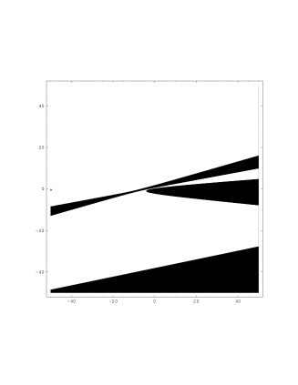
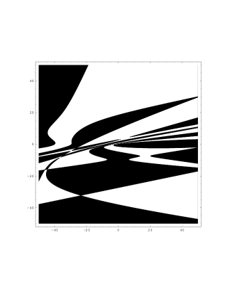
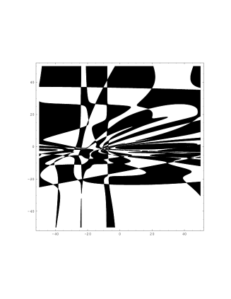
Figure 2: Sign[$\det M_{qb}$] at levels (4, 12), (6, 18), and (8, 16)

The results we have summarized here give good evidence that the level truncation method gives a good systematic approximation scheme for the location of the boundary of the region of Feynman-Siegel gauge validity near the origin in field space. In the remainder of this talk we discuss briefly a few applications of these results to the problem of tachyon condensation.

4 Applications to tachyon condensation

4.1 Branch points in tachyon effective potential

As discussed in Section 1, the calculations in [6] of the tachyon effective potential using the level-truncation method indicated the presence of two branch points in the effective potential, near $\phi\approx-0.25/g$ and $\phi\approx 1.5/g$. These calculations were performed using Feynman-Siegel gauge. The tachyon effective potential is computed by choosing a value of $\phi$, solving the equations of motion for all the other scalar fields, and computing the energy using these values for the fields. By following the trajectory in field space associated with this potential, we have found that as the tachyon value approaches the points associated with branch points of the effective potential, the field configuration given by solving the equations of motion for the other fields approaches the boundary of the region of Feynman-Siegel gauge validity. It is difficult to numerically follow the field trajectory close to the branch points since numerical methods become unstable in this region. By following the trajectory to a point near the branch point, and extrapolating the trajectory further along a quadratic curve matching the first and second derivatives of the computed curve, however, we find that at each level in level truncation, the value of $\phi$ where the trajectory crosses the Feynman-Siegel validity region comes within a few percent of the value where the effective potential encounters a branch point. An example of such a calculation is shown in Figure 3, where the determinant (13) is graphed as a function of $\phi$ along the trajectory of fields giving the effective potential at level $(4,12)$. The first branch point at this level is near $\phi\approx-0.286/g$, and the boundary of Feynman-Siegel gauge validity is encountered near this point. Calculating the determinant along the line of the effective potential to within $0.001/g$ of the branch point and continuing on a quadratic trajectory, we find that the boundary of the Feynman-Siegel validity region is encountered at $\phi\approx-0.290$, within $2\%$ of the branch point location. Similar results are found for the second branch point at level (4, 12) and for both branch points at other levels of truncation.

Figure 3: $\det M_{qb}$ in level (4, 8) truncation along tachyon potential.

This analysis gives strong evidence that the branch points in the tachyon effective potential encountered in [6] are gauge artifacts. Thus, cubic string field theory seems completely consistent with background independent string field theory, where the tachyon potential is unbounded below for sufficiently negative values of the tachyon field. We expect that if a method could be found for using cubic string field theory to compute the tachyon effective potential below the branch point $\phi\approx-0.25/g$ a similar result would be found.

4.2 Extra constraints on Feynman-Siegel gauge solution

Another interesting result which can be obtained from the level truncation of the full (non-gauge-fixed) SFT action is an infinite family of new constraints on the FS gauge nontrivial vacuum state. It is now generally believed that there is a well-defined state $\Phi_{0}$ in the Fock space which is annihilated by $b_{0}$ and which satisfies the SFT equation of motion $Q\Phi_{0}+g\Phi_{0}\star\Phi_{0}=0$. The coefficients of the low-level fields in this state were determined to a high degree of numerical accuracy in [1, 5, 6] by solving the equations of motion $\partial S/\partial\phi^{b}=0$ for all the fields associated with states annihilated by $b_{0}$. It should also be the case, however, that the equations of gauge invariance $\partial S/\partial\phi^{q}=0$ associated with states annihilated by $c_{0}$ should be satisfied in the nontrivial vacuum. This gives an infinite family of additional conditions which should be satisfied by $\Phi_{0}$. At any finite level of truncation, these additional equations of motion will only be satisfied approximately. For example, the equation of motion for the level two field $\eta$ in (2) vanishes in the stable vacuum to $92\%$ when only level two fields are considered, $98\%$ when level four fields are considered, and $99\%$ when level six fields are included. Related gauge invariance conditions for the vacuum were previously considered in [21, 22]; other algebraic constraints on the vacuum were found in [23, 24]. It is interesting to ask whether all these constraints can be combined to give a more efficient method for determining the stable vacuum.

4.3 Finding the vacuum without gauge fixing or in other gauges

Since we have found that the Feynman-Siegel gauge choice is only valid locally, it is interesting to ask whether we can find the true vacuum and/or the tachyon effective potential without gauge fixing. While in the complete theory there is an infinite-dimensional gauge orbit of equivalent locally stable vacua, the breakdown of gauge invariance caused by level truncation means that even without gauge fixing, the equations of motion of the level-truncated theory have only a discrete set of solutions. In the level (2, 6) truncation, for example, there are two solutions in the vicinity of the stable vacuum, with energy densities $E/VT_{25}=$ -0.880 and -1.078 (vs. -0.959 in FS gauge). (The first of these solutions was also found in [20]). At level (4, 12), there are at least three solutions, with $E/VT_{25}=$ -0.927, -0.963, and -1.075 (vs. -0.988 in FS gauge). As the level of truncation is increased, the multiplicity of the candidate solutions continues to grow. While some solutions approach the correct value, others do not, so without some further criterion for selecting branches, it does not seem possible to isolate a good candidate for the vacuum in the level-truncated, non-gauge-fixed theory. A unique branch of the effective potential at each level has the property that it can be determined by a power-series expansion of the equations of motion around the unstable vacuum, as was done in [6] for the FS gauge tachyon potential. Above level 4, however, this branch encounters a branch point before reaching the stable vacuum. This difficulty in solving the theory without gauge fixing clearly arises from the presence of a continuous family of equivalent vacua in the full theory.

While solving the theory numerically without gauge fixing does not seem practical, it is natural to ask whether other gauges may work as well or better than the Feynman-Siegel gauge for determining the stable vacuum or the effective tachyon potential. One simple way of modifying the Feynman-Siegel gauge choice, for example, is to choose a different set of fields to vanish at each level from those dictated by the Feynman-Siegel gauge choice. As long as these fields are associated with states in the image of $Q$ in the perturbative vacuum, this will locally be a valid gauge choice. As a simple example of such a different gauge choice, At level two we could choose to fix $B=0$ or $\beta=0$ instead of $\eta=0$. More generally, we could choose to set any linear combination of these fields to vanish which is not invariant under the linear terms in (9). We can then take the usual Feynman-Siegel gauge choice for all the higher-level fields. Each of these gauge choices defines a new gauge in which we can perform level truncated calculations to arbitrary level. We have tried a variety of gauges of this type. We find that in general, these gauges behave rather similarly to Feynman-Siegel gauge, although the vacuum energy in a generic gauge seems to converge somewhat more slowly than in Feynman-Siegel gauge. For example, using the gauge fixing $B=0$ for level two fields and FS gauge for all higher level fields, we find that $E/VT_{25}$ is given by $-0.901,-0.960,-0.979$ at levels (2, 6), (4, 12) and (6, 18) (compared to -0.959, -0.988, -0.995 in FS gauge). By choosing different fields to vanish at various low levels, we can choose a wide variety of gauges of this type. Tuning the coefficients of the linear combinations that are fixed to zero, we can produce a vacuum approximation at any particular level of truncation which has an energy density which is arbitrarily close to the desired value of $-VT_{25}$. In general, however, the approach to the vacuum energy is not monotonic, so this is not a particularly useful way to choose a gauge—even if the energy is exact at one level, including the next highest level of fields moves the energy away from the desired value by some small quantity.

The upshot of this investigation is that while various other gauges can be chosen which have similar behavior to Feynman-Siegel gauge, none seem to be particularly better than FS gauge, and generic other gauge choices seem to lack the property of monotonic convergence of the vacuum energy which seems empirically to characterize the FS gauge. It would be interesting to investigate other more general gauge choices, such as restricting to fields annihilated by some particular ghost operator other than $c_{0}$. This problem is left to future work.

5 Summary

We have investigated the range of validity of Feynman-Siegel gauge in Witten’s cubic string field theory. We found that this gauge choice breaks down outside a fairly small region in field space, and that the boundary of the region containing the origin in which Feynman-Siegel gauge is a good gauge choice can be stably computed using the level truncation method. We found that branch points appearing in earlier calculations of the tachyon effective potential are gauge artifacts arising when the field configuration along the effective potential leaves the region of validity of FS gauge. We investigated the possibility of determining the locally stable vacuum and/or the tachyon effective potential either without gauge fixing or by choosing a different gauge than Feynman-Siegel gauge, but found no approach which was substantially better than the Feynman-Siegel gauge-fixed approach.

References

- [1] V. A. Kostelecky and S. Samuel, “On a nonperturbative vacuum for the open bosonic string,” Nucl. Phys. B336 (1990) 263-296.
- [2] K. Bardakci and M. B. Halpern, “Explicit spontaneous breakdown in a dual model,” Phys. Rev. D10 (1974) 4230.
- [3] K. Bardakci, “Spontaneous symmetry breaking in the standard dual string model,” Nucl. Phys. B133 (1978) 297.
- [4] A. Sen, “Universality of the tachyon potential,” JHEP 9912, 027 (1999) hep-th/9911116.
- [5] A. Sen and B. Zwiebach, “Tachyon condensation in string field theory,” JHEP 0003, 002 (2000) hep-th/9912249.
- [6] N. Moeller and W. Taylor, “Level truncation and the tachyon in open bosonic string field theory,” Nucl. Phys. B 583, 105 (2000) hep-th/0002237.
- [7] A. A. Gerasimov and S. L. Shatashvili, “On exact tachyon potential in open string field theory,” JHEP 0010, 034 (2000) hep-th/0009103.
- [8] D. Kutasov, M. Marino and G. Moore, “Some exact results on tachyon condensation in string field theory,” JHEP 0010, 045 (2000) hep-th/0009148.
- [9] D. Ghoshal and A. Sen, “Normalisation of the background independent open string field theory action,” JHEP 0011, 021 (2000) hep-th/0009191.
- [10] J. A. Harvey and P. Kraus, “D-branes as unstable lumps in bosonic open string field theory,” JHEP 0004, 012 (2000), hep-th/0002117.
- [11] R. de Mello Koch, A. Jevicki, M. Mihailescu and R. Tatar, “Lumps and p-branes in open string field theory,” Phys. Lett. B 482, 249 (2000), hep-th/0003031.
- [12] N. Moeller, A. Sen and B. Zwiebach, “D-branes as tachyon lumps in string field theory,” JHEP 0008, 039 (2000), hep-th/0005036.
- [13] J. A. Harvey, “Komaba lectures on noncommutative solitons and D-branes,” hep-th/0102076.
- [14] I. Ellwood and W. Taylor, “Open string field theory without open strings,”, hep-th/0103085.
- [15] I. Ellwood, B. Feng, Y. He and N. Moeller, “The identity string field and the tachyon vacuum,” hep-th/0105024.
- [16] E. Witten, “Non-commutative geometry and string field theory,” Nucl. Phys. B268 (1986) 253.
- [17] D. J. Gross and A. Jevicki, “Operator formulation of interacting string field theory (I), (II),” Nucl. Phys. B283 (1987) 1; Nucl. Phys. B287 (1987) 225.
- [18] A. Leclair, M. E. Peskin and C. R. Preitschopf, “String field theory on the conformal plane (I)” Nucl. Phys. B317 (1989) 411-463.
- [19] M. R. Gaberdiel and B. Zwiebach, “Tensor constructions of open string theories 1., 2.,” Nucl. Phys. B505 (1997) 569, hep-th/9705038; Phys. Lett. B410 (1997) 151, hep-th/9707051.
- [20] L. Rastelli and B. Zwiebach, “Tachyon potentials, star products and universality,” hep-th/0006240.
- [21] H. Hata and S. Shinohara, “BRST invariance of the non-perturbative vacuum in bosonic open string field theory,” JHEP 0009, 035 (2000), hep-th/0009105.
- [22] P. Mukhopadhyay and A. Sen, “Test of Siegel gauge for the lump solution,” JHEP 0102, 017 (2001), hep-th/0101014.
- [23] B. Zwiebach, “Trimming the tachyon string field with SU(1,1),”, hep-th/0010190.
- [24] M. Schnabl, “Constraints on the tachyon condensate from anomalous symmetries,” Phys. Lett. B 504, 61 (2001), hep-th/0011238.