FTUAM-01/09; IFT-UAM/CSIC-01-15

hep-th/0105155

Getting just the Standard Model at Intersecting Branes
L. E. Ibáñez, F. Marchesano and R. Rabadán
Departamento de Física Teórica C-XI and Instituto de Física Teórica C-XVI,
Universidad Autónoma de Madrid, Cantoblanco, 28049 Madrid, Spain.
Abstract

1 Introduction

If string theory is to describe the observed physics, it should be possible to find string configurations containing the observed standard model (SM). In the last fifteen years it has been possible to construct string vacua with massless sector close to the SM with three quark/lepton generations [1]. However all string constructions up to now lead to extra massless fermions and/or gauge bosons in the low energy spectrum. The hidden reason for this fact is that all those constructions contain extra $U(1)$ (or non-Abelian) gauge symmetries beyond $SU(3)\times SU(2)\times U(1)_{Y}$ and the cancellation of gauge anomalies requires in general the presence of extra chiral fermions beyond the spectrum of the SM. The usual procedure in the literature is then to abandon the string theory techniques and use instead the low-energy effective Lagrangian below the string scale. Then one tries to find some scalar field direction in which all extra gauge symmetries are broken and extra fermions become massive. This requires a very complicated model dependent analysis of the structure of the scalar potential and Yukawa couplings and, usually, the necessity of unjustified simplifying assumptions. For example, there is a lot of arbitrariness in the choice of scalar flat directions and the physics varies drastically from one choice to another. Fundamental properties like proton stability typically result from the particular choice of scalar flat direction.

It is clear that it would be nice to have some string constructions with massless spectrum identical to that of the SM and with gauge group just $SU(3)\times SU(2)\times U(1)_{Y}$ already at the string theory level, without any effective field theory elaboration. This could constitute an important first step to the string theory description of the observed world. But it could also give us some model independent understanding of some of the mysteries of the SM like generation-replication or the stability of the proton.

In the present article we report on the first such string constructions yielding just the SM massless spectrum from the start. We consider the SM gauge group as arising from four sets of D-branes wrapping cycles on compactified (orientifolded) Type II string theory. At the intersections of the branes live chiral fermions to be identified with quarks and leptons. In order to obtain just the observed three generations of quarks and leptons the D-brane cycles have to intersect the appropriate number of times as shown in eq.(2.3). Models with quarks and leptons living at D-brane intersections were already considered in refs.[2, 3, 4, 5]. In those papers three generation models were obtained but involving either extra chiral fermions and $U(1)$’s beyond the SM [3, 4] or else an extended gauge group beyond the SM [5]. As we said, the models we report here have just the SM gauge group and there are no extra chiral fermions nor $U(1)$ gauge bosons.

The particular examples we discuss consist on sets of D6-branes wrapping on an orientifolded six-torus [6, 2] in the presence of a background NS B-field [5, 7, 8]. We classify the D6-brane cycles yielding the SM spectrum. We find certain families of models which depend on a few integer parameters. The analysis of the $U(1)$ gauge anomalies in the constructions, along the lines discussed in ref.[3], is crucial in obtaining the correct SM structure. In particular, we find that the four original gauge $U(1)$ symmetries can be identified with Baryon number, Lepton number, Peccei-Quinn symmetry and hypercharge (or linear combinations thereof). There are Wess-Zumino-like $B\wedge F$ couplings involving RR fields and the Abelian gauge bosons. Due to these couplings, three of the $U(1)$’s become massive (of order the string scale) and only a $U(1)$ remains in the massless spectrum. We discuss the conditions under which the remaining $U(1)$ symmetry is the standard hypercharge. This substantially constraints the structure of the configurations yielding $SU(3)\times SU(2)\times U(1)_{Y}$ as the only gauge group.

The D6-brane configurations we study are non-supersymmetric. However we show explicitly, extending a previous analysis in ref.[3], that for wide ranges of the parameters (compactification radii) there are no tachyonic scalars at any of the intersections. Thus at this level the configurations are stable. We also show that for certain values of the geometrical data (some brane distances and intersection angles) the required Higgs scalar multiplets may appear in the light spectrum. The obtained Higgs sector is quite analogous to the one appearing in the minimal supersymmetric standard model (MSSM). But in our case the parameters of the scalar potential have a geometrical interpretation in terms of the brane distances and angles. Since the models are non-supersymmetric, the string scale should then be of order 1-few TeV.

We find that all the SM configurations obtained have a number of common features which seem to be quite model independent and could be a general property of any string model yielding just the SM spectrum:

• A first property is the connection between the number of generations and the number of colours. Indeed, in order to cancel anomalies while having complete quark/lepton generations, the number of generations in the provided constructions must be equal to the number of colours, three. This is quite an elegant explanation for the multiplicity of generations: there is no way in which we could construct e.g., a D-brane model with just one generation.

• Baryon number is an exact symmetry in perturbation theory. Indeed, we mentioned that Baryon number is a gauged $U(1)$ symmetry of the models. Although naively anomalous, the anomalies are cancelled by a generalized Green-Schwarz [9] mechanism which at the same time gives a mass to the corresponding gauge boson. The corresponding $U(1)$ symmetry remains as an effective global symmetry in the effective Lagrangian. This is a remarkable simple explanation for the observed stability of the proton. Indeed, the standard explanation for the surprisingly high level of stability of the proton is to suppose that the scale of baryon number violation is extremely large, larger than $10^{16}$ GeV. This requires to postpone the scale of a more fundamental theory to a scale at least as large as $10^{16}$ GeV. In our present context the scale of fundamental physics may be as low as 1 TeV without any problem with proton stability. Thus, in particular, this provides a natural explanation for proton stability in brane-world models with a low (of order 1-few TeV) string scale [11, 12].

• Lepton number is an exact symmetry in perturbation theory. Again, Lepton number is a gauged symmetry and remains as a global symmetry in the effective action. This has the important consequence that Majorana neutrino masses are forbidden. On the other hand another generic feature of our class of models is the necessary presence of three generations of right-handed neutrinos (singlets under hypercharge). In general Dirac neutrino masses may be present and neutrinos may oscillate in the standard way since it is only the diagonal lepton number $L=L_{e}+L_{\mu}+L_{\tau}$ which is an exact symmetry.

• There is a generation-dependent Peccei-Quinn symmetry [13] which is also gauged and thus in principle remains as a global $U(1)$ symmetry in the effective Lagrangian.

In addition to these general properties, our class of models have other interesting features. We already mentioned that Higgs fields appear under certain conditions and that the Higgs sector comes in sets analogous to that of the Minimal Supersymmetric Standard Model (MSSM). There is no gauge coupling unification, the size of each gauge coupling constant is inversely proportional to the volume wrapped by the corresponding brane. Thus it seems one can reproduce the observed size of the gauge couplings by appropriately varying the compact volume. Yukawa couplings may be computed in terms of the area of the world-sheet stretching among the different branes. The dependence on this area is exponential, which may give an understanding [4] of the hierarchy of fermion masses. In the case of neutrino masses, one finds that they may be naturally small as a consequence of the PQ-like symmetry.

The structure of the present paper is as follows. In chapter 2 we describe the general philosophy in order to obtain the minimal spectrum of the SM at the intersections of wrapping D-branes. We also discuss the connection between the number of colours and generations in these constructions as well as the general structure of $U(1)$ anomaly cancellation. In chapter 3 we review the case of intersecting D6-branes wrapping on a six-torus and describe the spectrum as well as the general Green-Schwarz mechanism in these theories. The search for specific D6-brane configurations yielding just the SM spectrum is carried out in chapter 4. We present a classification of such type of models and study tadpole cancellation conditions. We also find the general conditions under which the $U(1)$ remaining light is the standard hypercharge.

In chapter 5 we study the stability of the brane configurations. Specifically we show the absence of tachyons for wide ranges of the compact radii. The spectrum of massive particles from KK and winding states is discussed in chapter 6. The appearance of Higgs fields in the light spectrum is discussed in chapter 7. We discuss the multiplicity of those scalars as well as the general structure of the mass terms appearing in the scalar potential. A brief discussion of the gauge coupling constants and the Yukawa couplings is offered in chapter 8. We leave chapter 9 for some final comments and conclusions.

2 The standard model intersection numbers

In our search for a string-theory description of the standard model (SM) we are going to consider configurations of D-branes wrapping on cycles on the six extra dimensions, which we will assume to be compact. Our aim is to find configurations with just the SM group $SU(3)\times SU(2)\times U(1)_{Y}$ as a gauge symmetry and with three generations of fermions transforming like the five representations:

$$Q_{L}^{i}=(3,2,1/6)\ ;\ U_{R}^{i}=({\bar{3}},1,-2/3)\ ;\ D_{R}^{i}=({\bar{3}},1,1/3)\ ;$$

$$L^{i}=(1,2,-1/2)\ ;\ E_{R}^{i}=(1,1,1)\ .$$ (2.1)

Now, in general, D-branes will give rise to $U(N)$ gauge factors in their world-volume, rather than $SU(N)$. Thus, if we have $r$ different stacks with $N_{i}$ parallel branes we will expect gauge groups in general of the form $U(N_{1})\times U(N_{2})\times....\times U(N_{r})$. At points where the D-brane cycles intersect one will have in general massless fermion fields transforming like bifundamental representations, i.e., like $(N_{i},{\bar{N}}_{j})$ or $(N_{i},N_{j})$. Thus the idea will be to identify these fields with the SM fermion fields.

A first obvious idea is to consider three types of branes giving rise in their world-volume to a gauge group $U(3)\times U(2)\times U(1)$. This in general turns out not to be sufficient. Indeed, as we said, chiral fermions like those in the SM appear from open strings stretched between D-branes with intersecting cycles. Thus e.g., the left-handed quarks $Q_{L}^{i}$ can only appear from open strings stretched between the $U(3)$ branes and the $U(2)$ branes. In order to get the right-handed leptons $E_{R}^{i}$ we would need a fourth set with one brane giving rise to an additional $U(1)^{\prime}$: the right-handed leptons would come from open strings stretched between the two $U(1)$ branes. Thus we will be forced to have a minimum of four stacks of branes with $N_{1}=3,N_{2}=2,N_{3}=1$ and $N_{4}=1$ yielding a $U(3)\times U(2)\times U(1)\times U(1)$ gauge group .

In the class of models we are considering the fermions come in bifundamental representations:

$$\sum_{a,b}n_{ab}(N_{a},{\overline{N}}_{b})+m_{ab}(N_{a},N_{b})+n_{ab}^{*}({\overline{N}}_{a},N_{b})+m_{ab}^{*}({\overline{N}}_{a},{\overline{N}}_{b})\ .$$ (2.2)

where here $n_{ab},n_{ab}^{*},m_{ab},m_{ab}^{*}$ are integer non-negative coefficients which are model dependent . In all D-brane models strong constraints appear from cancellation of Ramond-Ramond (RR) tadpoles. Cancellation of tadpoles also guarantees the cancellation of gauge anomalies. In the case of the D-brane models here discussed anomaly cancellation just requires that there should be as many $N_{a}$ as ${\overline{N}}_{a}$ representations for any $U(N_{a})$ group.

An important fact for our discussion later is that tadpole cancellation conditions impose this constraint even if the gauge group is $U(1)$ or $U(2)$. The constraint in this case turns out to be required for the cancellation of $U(1)$ anomalies. Let us now apply this to a possible D-brane model yielding $U(3)\times U(2)\times U(1)\times U(1)$ gauge group. Since $U(2)$ anomalies have to cancel we will make a distinction between $U(2)$ doublets and antidoublets. Now, in the SM only left-handed quarks and leptons are $SU(2)$ doublets. Let us assume to begin with that the three left-handed quarks $Q_{L}^{i}$ were antidoublets $(3,{\bar{2}})$. Then there are altogether 9 anti-doublets and $U(2)$ anomalies would never cancel with just three generations of left-handed leptons. Thus all models in which all left-handed quarks are $U(2)$ doublets (or antidoublets) will necessarily require the presence in the spectrum of 9 $U(2)$ lepton doublets (anti-doublets) . There is however a simple way to cancel $U(2)$ anomalies sticking to the fermion content of the SM. They cancel if two of the left-handed quarks are antidoublets and the third one is a doublet . Then there is a total of six doublets and antidoublets and $U(2)$ anomalies will cancel.

Notice that in this case it is crucial that the number of generations equals the number of colours. There is no way to build a D-brane configuration with the gauge group of the SM and e.g., just one complete quark/lepton generation. Anomalies (RR tadpoles) cannot possibly cancel. We find this connection between the number of generations and colours quite attractive.

From the above discussion we see that, if we want to stick to the particle content of the minimal SM , we will need to consider string configurations in which both types of bifundamental fermion representations, $(N_{a},{\bar{N}}_{b})$ and $(N_{a},N_{b})$ appear in the massless spectrum. This possibility is familiar from Type II orientifold [17, 18] models in which the world-sheet of the string is modded by some operation of the form $\Omega{\it R}$, where $\Omega$ is the world-sheet parity operation and ${\it R}$ is some geometrical action. Bifundamental representations of type $(N_{a},{\bar{N}}_{b})$ appear from open strings stretched between branes $a$ and $b$ whereas those of type $(N_{a},N_{b})$ appear from those going between branes $a$ and $b^{*}$, the latter being the mirror of the $b$ brane under the $\Omega{\it R}$ operation. We will thus from now on assume that we are considering string and brane configurations in which both types of bifundamentals appear. Specific examples will be considered in the following sections.

It is now clear what are we looking for. We are searching for brane configurations with four stacks of branes yielding an initial $U(3)\times U(2)\times U(1)\times U(1)$ gauge group. They wrap cycles $\Pi_{i}$, $i=a,b,c,d$ and intersect with each other a number of times given by the intersection numbers $I_{ij}=\Pi_{i}.\Pi_{j}$. In order to reproduce the desired fermion spectrum (depicted in table 1) the intersection numbers should be :

$$I_{ab}\ = \ 1\ ;\ I_{ab*}\ =\ 2$$

$$I_{ac}\ = \ -3\ ;\ I_{ac*}\ =\ -3$$

$$I_{bd}\ = \ 0\ ;\ I_{bd*}\ =\ -3$$

$$I_{cd}\ = \ -3\ ;\ I_{cd*}\ =\ 3$$ (2.3)

all other intersections vanishing. Here a negative number denotes that the corresponding fermions should have opposite chirality to those with positive intersection number. As we discussed, cancellation of $U(N_{i})$ anomalies requires:

$$\sum_{j}\,I_{ij}\,N_{j}=0$$ (2.4)

which is indeed obeyed by the spectrum of table 1, although to achieve this cancellation we have to add three fermion singlets $N_{R}$. As shown below these have quantum numbers of right-handed neutrinos (singlets under hypercharge). Thus this is a first prediction of the present approach: right-handed neutrinos must exist.

Intersection	Matter fields		$Q_{a}$	$Q_{b}$	$Q_{c}$	$Q_{d}$	Y
(ab)	$Q_{L}$	$(3,2)$	1	-1	0	0	1/6
(ab*)	$q_{L}$	$2(3,2)$	1	1	0	0	1/6
(ac)	$U_{R}$	$3({\bar{3}},1)$	-1	0	1	0	-2/3
(ac*)	$D_{R}$	$3({\bar{3}},1)$	-1	0	-1	0	1/3
(bd*)	$L$	$3(1,2)$	0	-1	0	-1	-1/2
(cd)	$E_{R}$	$3(1,1)$	0	0	-1	1	1
(cd*)	$N_{R}$	$3(1,1)$	0	0	1	1	0

Table 1: Standard model spectrum and $U(1)$ charges

The structure of the $U(1)$ gauge fields is very important in what follows. The following important points are in order:

1) The four $U(1)$ symmetries $Q_{a}$, $Q_{b}$, $Q_{c}$ and $Q_{d}$ have clear interpretations in terms of known global symmetries of the standard model. Indeed $Q_{a}$ is $3B$, $B$ being the baryon number and $Q_{d}$ is nothing but (minus)lepton number. Concerning $Q_{c}$, it is twice $I_{R}$, the third component of right-handed weak isospin familiar from left-right symmetric models. Finally $Q_{b}$ has the properties of a Peccei-Quinn symmetry (it has mixed $SU(3)$ anomalies). We thus learn that all these known global symmetries of the SM are in fact gauge symmetries in this class of theories.

2) The mixed anomalies $A_{ij}$ of these four $U(1)_{i}$’s with the non-Abelian groups $SU(N_{j})$ are given by:

$$A_{ij}\ =\ {1\over 2}\ (I_{ij}-I_{i*j})\ N_{i}\ .$$ (2.5)

It is easy to check that $(Q_{a}+3Q_{d})$ (which is $3(B-L)$) and $Q_{c}$ are free of triangle anomalies. In fact the hypercharge is given by the linear combination:

$$Q_{Y}\ =\ {1\over 6}Q_{a}\ -\ {1\over 2}Q_{c}\ +\ {1\over 2}Q_{d}$$ (2.6)

and is, of course, anomaly free. On the other hand the other orthogonal combinations $(3Q_{a}-Q_{d})$ and $Q_{b}$ have triangle anomalies. Of course, if the theory is consistent these anomalies should somehow cancel. What happens is already familiar from heterotic compactifications [19] and Type I and Type II theories in six [20] and four [21] dimensions. There will be closed string modes coupling to the gauge fields giving rise to a generalized Green-Schwarz mechanism. This will work in general as follows. Typically there are RR two-form fields $B_{\alpha}$ with couplings to the $U(1)_{i}$ field strengths:

$$\sum_{\alpha}c_{\alpha}^{i}\ B_{\alpha}\wedge tr(F^{i})$$ (2.7)

and in addition there are couplings of the Poincare dual scalars $\eta_{\alpha}$ of the $B_{\alpha}$ fields:

$$\sum_{\alpha}d_{\alpha}^{j}\eta_{\alpha}tr(F^{j}\wedge F^{j})$$ (2.8)

where $F^{j}$ are the field strengths of any of the gauge groups. The combination of both couplings cancels the mixed $U(1)_{i}$ anomalies with any other group $G_{j}$ as:

$$A_{ij}\ +\ \sum_{\alpha}c_{\alpha}^{i}d_{\alpha}^{j}\ =\ 0\ .$$ (2.9)

Notice two important points:

a) Given $i,j$, for anomalies to cancel both $c_{\alpha}^{i}$ and $d_{\alpha}^{j}$ have to be non-vanishing for some ${\alpha}$.

b) The couplings in (2.7) give masses to some combinations of $U(1)$’s. This always happens for anomalous $U(1)$’s since in this case both $c_{\alpha}^{i}$ and $d_{\alpha}^{j}$ are necessarily non-vanishing. However it may also happen for some anomaly-free $U(1)$’s for which the corresponding combination of $\eta_{\alpha}$ fields does not couple to any $F\wedge F$ piece.

In our case the $(3Q_{a}-Q_{d})$ and $Q_{b}$ gauge bosons will become massive. On the other hand the other two anomaly free combinations (including hypercharge) may be massive or not, depending on the couplings $c_{\alpha}^{i}$. Thus in order to really obtain a standard model gauge group with the right standard hypercharge we will have to insure that it does not couple to any closed string mode which would render it massive, i.e., one should have

$$\sum_{\alpha}\ ({1\over 6}c_{\alpha}^{a}\ -\ {1\over 2}c_{\alpha}^{c}\ +\ {1\over 2}c_{\alpha}^{d}\ )\ =\ 0$$ (2.10)

This turns out to be an important constraint in the specific models constructed in the following sections. But an important conclusion is that in those models generically only three of the four $U(1)$’s can become massive and that in a large subclass of models it is the SM hypercharge which remains massless. Thus even though we started with four $U(1)$’s we are left at the end of the day with just the SM gauge group.

Let us also remark that the symmetries whose gauge boson become massive will persist in the low-energy spectrum as global symmetries . This has important obvious consequences, as we will discuss below.

Up to now we have been relatively general and perhaps a structure like this may be obtained in a variety of string constructions. We believe that the above discussion identifies in a clear way what we should be looking for in order to get a string construction with a massless sector identical to the SM. In the following sections we will be more concrete and show how this philosophy may be followed in a simple setting. Specifically, we will be considering Type IIA D6-branes wrapping at angles [2] on a six torus $T^{6}$. We will see how even in such a simple setting one can obtain the desired structure.

3 D6-branes intersecting at angles

Let us consider D6-branes wrapping homology 3-cycles on a six dimensional manifold $\cal M$. Some general features of this construction do not depend on the specific choice of metric on this space but only on the homology of these three cycles and its intersection form. More concrete problems, as the supersymmetry preserved by the configuration or the presence of tachyons on it, will depend on the metric. We will discuss first some of these abstract properties to proceed later to review the toroidal case in detail.

Two D6-branes on three-cycles will intersect generically at a finite number of points and those intersections will be four-dimensional. The intersection number depends on the homology class of the cycles. Deforming the D-branes within the same homology class the intersection number does not change. Let us take a basis for the $H_{3}({\cal M},Z\kern-3.99994ptZ)$, $\Sigma_{i}$, where $i=1,\dots,b_{3}$ and $b_{3}$ is the correspondent Betti number. Let us call $C_{ij}$ the intersection number of the cycles $\Sigma_{i}$ and $\Sigma_{j}$. Some properties will depend only on the homology of the cycles, $\Pi_{a}$, where the D-branes are living:

• there is a massless $U(1)$ field on each brane that can be enhanced to a $U(N)$ if N of these D-brane coincide. Some of the $U(1)$ factors will be massive due to the WZ couplings.

• There is a chiral fermion [22, 23] at each four-dimensional intersection between the cycles $\Pi_{a}$, $\Pi_{b}$ transforming in the bifundamental of $U(N_{a})\times U(N_{b})$, where the specific chirality depends on the sign of the intersection, and the number represents the multiplicity.

• There are some conditions related to the propagation of RR massless closed string fields on the compact space. These are the RR tadpoles. These tadpoles can be expressed in a very simple way: the sum of the cycles where the branes are living must vanish [24, 3]:

  $$\sum_{a}^{K}N_{a}\Pi_{a}=0$$ (3.1)

  In the presence of additional sources for RR charge (e.g., orientifold planes) one should add the corresponding contribution (see the toroidal example below). RR tadpoles imply the cancellation of all abelian gauge anomalies. Tadpoles of the particles in the NSNS sector are in general not cancelled (unless the configuration preserves some supersymmetry).

• Some of the above $U(1)$ gauge fields will be anomalous and the anomalies are expected to cancel in the way described in the previous section. The triangle anomaly can be computed directly from the chiral spectrum, and after imposing tadpole cancellation conditions (3.1) one gets for the $SU(N_{b})^{2}\times U(1)_{a}$ anomaly:

  $$A_{ab}=\frac{1}{2}N_{a}(\Pi_{a}.\Pi_{b})$$ (3.2)

where $(\Pi_{a}.\Pi_{b})$ is the intersection number of the $\Pi_{a}$ and $\Pi_{b}$ cycles.

As we have mentioned above other properties as the presence or absence of tachyons, the supersymmetries preserved [25, 26, 27] by the system of D-branes, the massive spectrum, etc. will depend on the specific choice of metric, B-field and other background values.

3.1 D6-branes on a torus

Let us consider a particular example of the above ideas : D6-branes wrapping a three cycle on a six dimensional torus. A more specific choice consists on a factorization of the six dimensional torus into $T^{2}\times T^{2}\times T^{2}$. We can wrap a D6-brane on a 1-cycle of each $T^{2}$ so it expands a three dimensional cycle on the whole $T^{6}$ . Let us denote by $(n_{a}^{i},m_{a}^{i})$ the wrapping numbers of the $D6_{a}$-brane on the $i$-th $T^{2}$. We refer the reader to refs.[2, 5] where these kind of configurations have been studied in detail.

The metric on each $T^{2}$ is constant and can be parametrized by a couple of fields: the complex structure $U$ and the complexified Kahler form $J$. The complexification of the Kahler form is done by taking in addition with the area the B-field value. The above models have a T-dual description in terms of D9-branes with magnetic fluxes. The T-duality transformation can be carried out in each $T^{2}$ separately. A D-brane wrapped on a $(n,m)$ is mapped to a $U(n)$ field with a constant field strength $F$ whose first Chern class is m. The D6-brane boundary conditions

$$\sin\vartheta_{a}^{I}\partial_{\sigma}X_{1}^{I}-\cos\vartheta_{a}^{I}\partial_{\sigma}X_{2}^{I} = 0$$

$$\sin\vartheta_{a}^{I}\partial_{\tau}X_{2}^{I}-\cos\vartheta_{a}^{I}\partial_{\tau}X_{1}^{I} = 0$$ (3.3)

are translated into [2]

$$\partial_{\sigma}X_{1}^{I}-F_{a}^{I}\partial_{\tau}X_{2}^{I} = 0$$

$$\partial_{\sigma}X_{2}^{I}-F_{a}^{I}\partial_{\tau}X_{1}^{I} = 0$$ (3.4)

in the T-dual picture . The flux $F$ is related to the angle between the brane and the direction where T-duality is performed $F_{a}^{I}=\cot{\vartheta_{a}^{I}}$. T-duality on the three two tori takes the D6-brane system to a system with D9-branes with fluxes and the complex structure and complexified Kahler form interchanged. On this paper we will use the D6-branes at angles picture because it is easier to visualize the specific brane constructions.

3.1.1 Orientifolds

Let us start from Type I string theory with branes with fluxes on a six dimensional torus [6, 2]. Perform a T-duality on the $x^{4}$, $x^{6}$, $x^{8}$ directions. The world sheet parity $\Omega$ is mapped into $\Omega{\cal R}$ where ${\cal R}$ is a reflection on the T-dualized coordinated $x^{4}$, $x^{6}$ and $x^{8}$. The D9-branes with fluxes are translated into D6-branes at angles. Consistency with the $\Omega{\cal R}$ symmetry requires the D6-branes to be in pairs: if $(n,m)$ are the wrapping numbers of a brane along a two dimensional torus, there must be a $\Omega{\cal R}$ partner wrapping the cycle $(n,-m)$ (See figure 1). Let us denote by $\Omega{\cal R}D_{a}$6-brane the $\Omega{\cal R}$ image of the brane $D_{a}$6-brane.

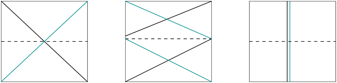
Figure 1: The $\Omega{\cal R}$ world sheet parity takes one set of branes specified by $(n_{i},m_{i})$ to another set $(n_{i},-m_{i})$. The dashed line represent the direction where the O6-plane lives.

The spectrum can be easily obtained by taking $\Omega{\cal R}$ invariant combinations. There are several sectors to be taken into account [2]:

• $D_{a}-D_{a}$: the $\Omega{\cal R}$ takes this sector to the $\Omega{\cal R}D_{a}-\Omega{\cal R}D_{a}$ sector. In general these sectors will be different and one should only take one of these into account. This sector contains, as in the toroidal case, d=4 ${\cal N}=4$ super Yang-Mills. When one brane is its own orientifold image $SO(N)$ and $USp(N)$ groups can appear (See, for instance, [2].). As we are interested in unitary groups we will not consider these cases.

• $D_{a}-D_{b}$: the $\Omega{\cal R}$ takes this sector to the $\Omega{\cal R}D_{b}-\Omega{\cal R}D_{a}$ sector. One obtains chiral fermions in the bifundamental $(N_{a},\bar{N}_{b})$ of the group with multiplicity given by the intersection number :

  $$I_{ab}\ =\ (n_{a}^{1}m_{b}^{1}-m_{a}^{1}n_{b}^{1})(n_{a}^{2}m_{b}^{2}-m_{a}^{2}n_{b}^{2})(n_{a}^{3}m_{b}^{3}-m_{a}^{3}n_{b}^{3})$$ (3.5)

• $D_{a}-\Omega{\cal R}D_{b}$: this sector is taken to the $D_{b}-\Omega{\cal R}D_{a}$ sector. There are chiral fermions in the $(N_{a},N_{b})$ representation with multiplicity

  $$I_{ab^{*}}\ =\ -(n_{a}^{1}m_{b}^{1}+m_{a}^{1}n_{b}^{1})(n_{a}^{2}m_{b}^{2}+m_{a}^{2}n_{b}^{2})(n_{a}^{3}m_{b}^{3}+m_{a}^{3}n_{b}^{3})\ .$$ (3.6)

  In eqs.(3.5) and (3.6) a negative sign implies opposite chirality.

• $D_{a}-\Omega{\cal R}D_{a}$: this sector is taken to the $D_{a}-\Omega{\cal R}D_{a}$ sector. This is an invariant sector so the $\Omega{\cal R}$ projection should be imposed on it: some of the intersections will be invariant and the others will be in pairs. The invariant ones give $8m_{a}^{1}m_{a}^{2}m_{a}^{3}$ fermions in the antisymmetric representation and the others produce $4m_{a}^{1}m_{a}^{2}m_{a}^{3}(n_{a}^{1}n_{a}^{2}n_{a}^{3}-1)$ symmetric and antisymmetric representations [2] .

RR tadpole conditions can be easily obtained from the toroidal case taking into account that some of the conditions are immediately satisfied because the pairs of branes cancel the contribution to some cycle conditions (the cycles with an odd number of $m_{i}$’s). The orientifold plane introduces a net RR charge in the $(1,0),(1,0),(1,0)$ cycle. So the tadpole conditions read

$$\sum_{a}N_{a}n_{a}^{1}n_{a}^{2}n_{a}^{3}=16$$

$$\sum_{a}N_{a}m_{a}^{1}m_{a}^{2}n_{a}^{3}=0$$

$$\sum_{a}N_{a}m_{a}^{1}n_{a}^{2}m_{a}^{3}=0$$

$$\sum_{a}N_{a}n_{a}^{1}m_{a}^{2}m_{a}^{3}=0$$ (3.7)

One can also consider the possibility of adding a NS B-flux [7], $b^{i}$, to each two dimensional torus in the D9-brane picture [5]. The total flux in the brane becomes a combination of the magnetic and B-field flux, ${\cal F}=b+F$. In the T-dual picture the torus changes its complex structure in such a way that it takes into account the modified angle of the brane ${\cal F}=\cot{\vartheta}$. Notice that the B-field is not invariant under $\Omega$. It is not a dynamical field but some discrete values are allowed: $b=0,1/2$. In the T-dual picture the B-field is translated into a fixed complex structure [5]. In an effective manner the addition of this B-background allows for semi-integer $m^{i}$ values. If originally the wrapping numbers on a torus are $(n,m^{\prime})$, the effective wrapping numbers upon the addition of a $b=1/2$ background are $(n,m^{\prime}+n/2)$ [5]. In what follows we will denote by $m=m^{\prime}+n/2$ in those tori with a B-background.

3.2 $U(1)$ Anomaly cancellation

Anomaly cancellation of $U(1)$’s for toroidal models were already considered in ref.[3]. In the orientifold case here considered there are some simplifications compared to the toroidal case. Let us consider the T-dual version consisting of Type I string theory (D9-branes) with magnetic fluxes. We have in ten dimensions RR fields $C_{2}$ and $C_{6}$ only with world-volume couplings (wedge products are understood) :

$$\int_{D9_{a}}C_{6}\,F_{a}^{2}\ ;\ \int_{D9_{a}}C_{2}\,F_{a}^{4}\ .$$ (3.8)

Upon dimensional reduction we get one two form plus three other two-forms:

$$B_{2}^{0} = C_{2}$$

$$B_{2}^{I} = \int_{(T^{2})_{J}\times(T^{2})_{K}}C_{6}\ ;I=1,2,3$$ (3.9)

with $I\not=J\not=K\not=I$ and their four-dimensional duals:

$$C^{0} = \int_{(T^{2})_{1}\times(T^{2})_{2}\times(T^{2})_{3}}C_{6}$$

$$C^{I} = \int_{(T^{2})_{I}}C_{2}\$$ (3.10)

with $dC^{0}=-*dB_{2}^{0}$ and $dC^{I}=-*dB_{2}^{I}$. These RR fields have four-dimensional couplings to the gauge fields given by [3]:

$$\begin{array}[]{ccc}N_{a}\,m^{1}_{a}\,m^{2}_{a}\,m^{3}_{a}\int_{M_{4}}B_{2}^{0}\wedge F_{a}&\quad;&n^{1}_{b}\,n^{2}_{b}\,n^{3}_{b}\int_{M_{4}}C^{0}\wedge F_{b}\wedge F_{b}\\ N_{a}\,n^{J}_{a}\,n^{K}_{a}\,m^{I}_{a}\int_{M_{4}}B_{2}^{I}\wedge F_{a}&\quad;&n^{I}_{b}\,m^{J}_{b}\,m^{K}_{b}\int_{M_{4}}C^{I}\wedge F_{b}\wedge F_{b}\ .\end{array}$$ (3.12)

The Green-Schwarz amplitude where $U(1)_{a}$ couples to one of the $B_{2}$ RR fields which propagates and couples to two $SU(N_{b})$ gauge bosons will be proportional to:

$$-N_{a}\,\;m^{1}_{a}m^{2}_{a}m^{3}_{a}n^{1}_{b}n^{2}_{b}n^{3}_{b}\ -\ N_{a}\,\sum_{I}n^{I}_{a}n^{J}_{a}m^{K}_{a}n^{K}_{b}m^{I}_{b}m^{J}_{b}\ ,\ I\not=J,K$$ (3.13)

which precisely has the form to cancel the triangle anomalies. Notice that due to the linear couplings between the $U(1)$’s and the RR two-forms some of the $U(1)$’s (including all those which are anomalous) will become massive. Since there are only four two-forms available, in any model with any arbitrary number of branes only a maximum of four $U(1)$’s may become massive. Notice also that in any realistic model we will have to ensure that the physical hypercharge generator is not one of them.

4 Searching for the standard model

Let us try to construct a specific model with low-energy spectrum given by that in table 1, corresponding to the intersection numbers in eq.(2.3). We find that getting the spectrum of the SM is quite a strong constraint. We find families of models corresponding to choices of wrapping numbers $n_{i}^{l}$, $m_{i}^{l}$, $i=a,b,c,d$, $l=1,2,3$ as well as adding a NS $B$-background or not on the three underlying tori. To motivate the form of these solutions let us enumerate some of the constraints we have to impose:

1) We will require that for any brane $i$ one has $\Pi_{l=1}^{3}\ m_{i}^{l}\ =0$ because of two reasons. First, to avoid the appearance of matter at the intersections of one brane to its mirror. This matter (transforming like symmetric or antisymmetric representations of the gauge group) has exotic quantum numbers beyond the particle content of the SM which we are trying to reproduce. In addition, there are tachyonic scalars at those intersections which would destabilize the brane configuration.

2) If $\Pi_{l=1}^{3}\ m_{i}^{l}\ =0$ is verified, then in these toroidal models there are only at most three RR fields $B^{l}$, $l=1,2,3$ with couplings to the Abelian groups. Thus at most three $U(1)$’s may become massive by the mechanism described in chapter 2. This implies that we should consider only models with four sets of branes at most, since otherwise there would be additional massless $U(1)$ gauge bosons beyond hypercharge.

3) We further impose that we should reproduce the spectrum in table 1. This is the most constraining condition. It implies that the branes $a$ should be parallel to the $d$ brane in at least one of the three complex planes and that the $b$ branes are parallel to the $c$ brane. Getting $I_{ab}=1$ and $I_{ab^{*}}=2$ requires that at least one of the three tori (e.g.,the third) should be tilted (or should have a b-background, in the T-dual language). Getting the other intersection numbers correct gives us also further constraints.

Imposing these conditions we find the general class of solutions for the wrapping numbers shown in table (2).

$N_{i}$	$(n_{i}^{1},m_{i}^{1})$	$(n_{i}^{2},m_{i}^{2})$	$(n_{i}^{3},m_{i}^{3})$
$N_{a}=3$	$(1/\beta^{1},0)$	$(n_{a}^{2},\epsilon\beta^{2})$	$(1/\rho,1/2)$
$N_{b}=2$	$(n_{b}^{1},-\epsilon\beta^{1})$	$(1/\beta^{2},0)$	$(1,3\rho/2)$
$N_{c}=1$	$(n_{c}^{1},3\rho\epsilon\beta^{1})$	$(1/\beta^{2},0)$	$(0,1)$
$N_{d}=1$	$(1/\beta^{1},0)$	$(n_{d}^{2},-\beta^{2}\epsilon/\rho)$	$(1,3\rho/2)$

Table 2: D6-brane wrapping numbers giving rise to a SM spectrum. The general solutions are parametrized by a phase $\epsilon=\pm 1$, the NS background on the first two tori $\beta^{i}=1-b^{i}=1,1/2$, four integers $n_{a}^{2},n_{b}^{1},n_{c}^{1},n_{d}^{2}$ and a parameter $\rho=1,1/3$. In order to obtain the correct hypercharge massless $U(1)$ those parameters have to verify the extra constraint eq.(4.6).

In the table we have $\beta^{i}=1-b^{i}$, with $b^{i}=0,1/2$ being the NS B-background field discussed in section 3. In the third torus one always has $b^{3}=1/2$. Also $\epsilon=\pm 1$ and $\rho$ takes only the values $\rho=1,1/3$. Notice that each of these families of D6-brane configurations depends on four integers ($n_{a}^{2},n_{b}^{1},n_{c}^{1}$ and $n_{d}^{2}$) . All of the choices lead exactly to the same massless fermion spectrum of table 1.

One has now to ensure that these choices are consistent with the tadpole cancellation conditions described in the previous section. It turns out that all but the first of those conditions are automatically satisfied by the above families of configurations. The first tadpole condition reads in the present case:

$$\frac{3n_{a}^{2}}{\rho\beta^{1}}\ +\ \frac{2n_{b}^{1}}{\beta^{2}}\ +\ \frac{n_{d}^{2}}{\beta^{1}}\ =\ 16\ .$$ (4.1)

Note however that one can always relax this constraint by adding extra D6-branes with no intersection with the SM ones and not contributing to the rest of the tadpole conditions. For example, a simple possibility would be the addition $N_{h}$ D6 branes with $m_{h}^{l}=0$, i.e., parallel to the orientifold plane. In this case the above condition would be replaced by the more general one

$$\frac{3n_{a}^{2}}{\rho\beta^{1}}\ +\ \frac{2n_{b}^{1}}{\beta^{2}}\ +\ \frac{n_{d}^{2}}{\beta^{1}}\ +\ N_{h}n_{h}^{1}n_{h}^{2}n_{h}^{3}\ =\ 16\ .$$ (4.2)

Thus the families of standard model configurations we have found are very weakly constrained by tadpole cancellation conditions. This is not so surprising. Tadpole cancellation conditions are closely connected to cancellation of anomalies. Since the SM is anomaly-free, it is not surprising that the solutions we find almost automatically are tadpole-free.

Let us now analyze the general structure of $U(1)$ anomaly cancellation in this class of models. As we remarked in section 2, there are two anomalous $U(1)$’s given by the generators $(3Q_{a}-Q_{d})$ and $Q_{b}$ and two anomaly free ones which are $(Q_{a}+3Q_{d})$ and $Q_{c}$. Following the general discussion in previous section one can see that the three RR fields $B_{2}^{I}$, $l=1,2,3$ couple to the $U(1)$’s in the models as follows:

$$B_{2}^{1} \wedge \ {{-2\epsilon\beta^{1}}\over{\beta^{2}}}F^{b}$$

$$B_{2}^{2} \wedge \ \frac{(\epsilon\beta^{2})}{\rho\beta^{1}}(3F^{a}\ -\ F^{d})$$

$$B_{2}^{3} \wedge \ {1\over{2\beta^{2}}}(\frac{3\beta^{2}n_{a}^{2}}{\beta^{1}}F^{a}\ +\ 6\rho n_{b}^{1}F^{b}\ +\ 2n_{c}^{1}F^{c}\ +\ \frac{3\rho\beta^{2}n_{d}^{2}}{\beta^{1}}F^{d})\$$ (4.3)

whereas the $B_{2}^{0}$ RR field has no couplings to the $F_{j}$, because $\Pi_{l}m_{j}^{l}=0$ for all the branes. The dual scalars $C^{I}$ and $C^{0}$ have couplings:

$$C^{1}\ (\frac{\epsilon\beta^{2}}{2\beta^{1}}) (F^{a}\wedge F^{a}\ -\ 3F^{d}\wedge F^{d})$$

$$C^{2}\ (\frac{3\rho\epsilon\beta^{1}}{2\beta^{2}}) (-F^{b}\wedge F^{b}\ +\ 2F^{c}\wedge F^{c})$$ (4.4)

$$C^{0} (\frac{n_{a}^{2}}{\rho\beta^{1}}F^{a}\wedge F^{a}\ +\ \frac{n_{b}^{1}}{\beta^{2}}F^{b}\wedge F^{b}\ +\ \frac{n_{d}^{2}}{\beta^{1}}F^{d}\wedge F^{d})\$$

and the RR scalar $C^{3}$ does not couple to any $F\wedge F$ term. It is easy to check that these terms cancel all residual $U(1)$ anomalies in the way described in section 2. Notice in particular how only the exchange of the $B_{2}^{1},B_{2}^{2}$ fields (and their duals $C^{1},C^{2}$) can contribute to the cancellation of anomalies since the $C^{3}$ field does not couple to $F\wedge F$ and $B_{2}^{0}$ does not couple to any $F^{j}$. The exchange of those RR fields proceeds in a universal manner (i.e., independent of the particular choice of $n$’s) and hence the mechanism for the $U(1)$ anomalies to cancel is also universal. On the other hand the $B_{2}^{3}$ field does couple to a linear combination of the four $U(1)$’s and hence will render that combination massive. The $U(1)$ which remains light is given by the linear combination

$$Q\ =\ n_{c}^{1}(Q_{a}+3Q_{d})\ -\ {{3\beta^{2}}\over{2\beta^{1}}}(n_{a}^{2}+3\rho n_{d}^{2})Q_{c}$$ (4.5)

If we want to have just the standard hypercharge at low energies this should be proportional to the hypercharge generator. This is the case as long as:

$$n_{c}^{1}\ =\ {{\beta^{2}}\over{2\beta^{1}}}(n_{a}^{2}+3\rho n_{d}^{2})$$ (4.6)

which is an extra condition the four integers should fulfill in order to really obtain a SM at low energies. Thus we have found families of toroidal models with D6-branes wrapping at angles in which the residual gauge group is just the standard model $SU(3)\times SU(2)\times U(1)_{Y}$ and with three standard generations of quarks and leptons and no extra chiral fermions (except for three right-handed neutrinos which are singlets under hypercharge).

These models are specific examples of the general approach in section 2. Notice in particular that in these models Baryon number ($Q_{a})$, and lepton number ($Q_{d}$) are unbroken gauged $U(1)$ symmetries. The same is the case of the symmetry $Q_{b}$ which is a (generation dependent) Peccei-Quinn symmetry. Once the RR-fields give masses to three of the $U(1)$’s of the models, the corresponding $U(1)$’s remain as effective global symmetries in the theory. This has the important physical consequences:

1) Baryon number is an exact perturbative symmetry of the effective Lagrangian. Thus the nucleon should be stable. This is a very interesting property which is quite a general consequence of the structure of the theory in terms of D-branes intersecting at angles and which was already advanced in ref.[4]. Notice that this property is particularly welcome in brane scenarios with a low energy string scale [11, 12] in which stability of the proton is an outstanding difficulty. But it is also a problem in standard scenarios like the MSSM in which one has to impose by hand discrete symmetries like R-parity or generalizations in order to have a sufficiently stable proton.

2) Lepton number is an exact symmetry in perturbation theory. This has as a consequence that Majorana masses for the neutrinos should be absent. Any neutrino mass should be of standard Dirac type. They can however be naturally small as we discuss below.

3) There is a gauged $U(1)$ symmetry of the Peccei-Quinn type ($Q_{b}$) which is exact at this level. Thus, at this level the $\theta_{QCD}$ parameter can be rotated to zero.

These properties seem to be quite model independent, and also seem to be a generic property of any D-brane model which gives rise to just a SM spectrum at the intersections.

As a final comment note that the pseudoscalar $C^{0}$ remains massless at this level and has axionic couplings (eq.(4.4)) to the gauge fields of the SM (and also to the fields coming from the extra branes added to cancel tadpoles, if present). It would be interesting to study the possible relevance of this axion-like field concerning the strong CP problem.

5 Absence of tachyons and stability of the configurations

We have been concerned up to now with the massless chiral fermions at the D-brane intersections. In addition to those there are scalar states at each intersection which in some sense may be considered (in a sense specified below) ”SUSY-partners”, squarks and sleptons, of the massless chiral fermions, since they have the same multiplicity $|I_{ij}|$ and carry the same gauge quantum numbers . The lightest of those states have masses [3]

$$\begin{array}[]{cc}{\rm\bf State}&\quad{\bf Mass^{2}}\\ t_{1}=(-1+\vartheta_{1},\vartheta_{2},\vartheta_{3},0)&\alpha^{\prime}{\rm(Mass)}^{2}=\frac{1}{2}(-\vartheta_{1}+\vartheta_{2}+\vartheta_{3})\\ t_{2}=(\vartheta_{1},-1+\vartheta_{2},\vartheta_{3},0)&\alpha^{\prime}{\rm(Mass)}^{2}=\frac{1}{2}(\vartheta_{1}-\vartheta_{2}+\vartheta_{3})\\ t_{3}=(\vartheta_{1},\vartheta_{2},-1+\vartheta_{3},0)&\alpha^{\prime}{\rm(Mass)}^{2}=\frac{1}{2}(\vartheta_{1}+\vartheta_{2}-\vartheta_{3})\\ t_{4}=(-1+\vartheta_{1},-1+\vartheta_{2},-1+\vartheta_{3},0)&\alpha^{\prime}{\rm(Mass)}^{2}=1-\frac{1}{2}(\vartheta_{1}+\vartheta_{2}+\vartheta_{3})\end{array}$$ (5.6)

in the notation of ref.[3]. Here $\vartheta_{i}$ are the intersection angles (in units of $\pi$) at each of the three subtori. As is obvious from these formulae the masses depend on the angles at each intersection and hence on the relative size of the radii. Thus in principle some of the scalars may be tachyonic . In fig.2 we show the range of $\vartheta_{i}$ for which there are no tachyons at a given intersection.

Figure 2: The region inside the tetrahedron has no tachyons. Faces, edges and vertices represent respectively, ${\cal N}=1$, ${\cal N}=2$ and ${\cal N}=4$ systems at the given intersection.

There is a region (inside the tetrahedron) where all the scalars have positive $(mass)^{2}$. Supersymmetry is not preserved but the absence of tachyons indicates that the system cannot decay into another one that lowers the energy. Outside this region some scalars become tachyonic. The boundary between the two regions represents a supersymmetric configuration at that intersection. This boundary has a tetrahedral shape. The faces represent configurations that preserve ${\cal N}=1$, the edges correspond to ${\cal N}=2$ configurations and the vertices to ${\cal N}=4$ configurations at that particular intersection. At each of the faces a different scalar becomes massless and hence becomes degenerate with the chiral fermion in the intersection. One can check that if none of the other scalars is tachyonic there is a fermion-boson degeneration that indicates that one supersymmetry is preserved locally. It is in this sense that these scalars are SUSY-partners of the massless chiral fermion. At the edges it is two scalars (and one fermion) which become massless and one has (locally) ${\cal N}=2$ supersymmetry.

For a D-brane configuration to be stable there should be no tachyons at none of the intersections. As already noted in ref.[3], in general it is possible to vary the compact radii in order to get rid of all tachyons of a given model. One can do a general analysis of sufficient conditions for absence of tachyons in the standard model examples of previous sections which are parametrized in terms of $\beta^{1,2}$ and the integers $n_{a}^{2},n_{b}^{1},n_{c}^{1}$ and $n_{d}^{2}$. Let us define the angles

$$\theta_{1}\ =\ \frac{1}{\pi}cot^{-1}\frac{n_{b}^{1}R_{1}^{(1)}}{\beta^{1}R_{2}^{(1)}}\ ;\ \theta_{2}\ =\ \frac{1}{\pi}cot^{-1}\frac{n_{a}^{2}R_{1}^{(2)}}{\beta^{2}R_{2}^{(2)}}\ ;\ \theta_{3}\ =\ \frac{1}{\pi}cot^{-1}\frac{2R_{1}^{(3)}}{\rho R_{2}^{(3)}}$$

$${\tilde{\theta_{1}}}\ =\ \frac{1}{\pi}cot^{-1}\frac{|n_{c}^{1}|R_{1}^{(1)}}{3\rho\beta^{1}R_{2}^{(1)}}\ ;\ {\tilde{\theta_{2}}}\ =\ \frac{1}{\pi}cot^{-1}\frac{\rho n_{d}^{2}R_{1}^{(2)}}{\beta^{2}R_{2}^{(2)}}\ ;\ {\tilde{\theta_{3}}}\ =\ \frac{1}{\pi}cot^{-1}\frac{2R_{1}^{(3)}}{3\rho R_{2}^{(3)}}$$ (5.7)

where $R^{(i)}_{1,2}$ are the compactification radii for the three $i=1,2,3$ tori . The geometrical meaning of the angles is depicted in fig.(3).

Figure 3: Definition of the angles between the different branes on the three tori. We have selected a particular setting where $n_{a}^{2},n_{b}^{1},n_{c}^{1},n_{d}^{2}>0$, $\epsilon=-1$ and $\beta^{1}=1/2$, $\beta^{2}=1$.

Angles at all the intersections may be written in terms of those six angles which depend on the parameters of the particular model and the relative radii. We have four (possibly light) scalars $t_{i},i=1,2,3,4$ at each of the 7 independent types of intersections, thus altogether 28 different scalar masses. Since all these 28 masses can be written in terms of the above 6 angles, it is obvious that the masses are not all independent. Thus for example one finds:

$$m^{2}_{ab}(t_{2})+m^{2}_{ac}(t_{3})\ =\ m^{2}_{ab*}(t_{2})+m^{2}_{ac*}(t_{3})\ =\ m^{2}_{bd*}(t_{2})+m^{2}_{cd*}(t_{3})$$

$$m^{2}_{ab}(t_{1})+m^{2}_{ac}(t_{4})\ =\ m^{2}_{ab*}(t_{1})+m^{2}_{ac*}(t_{4})\ =\ m^{2}_{bd*}(t_{1})+m^{2}_{cd*}(t_{4})$$

$$m^{2}_{ab}(t_{1})+m^{2}_{ac*}(t_{2})\ =\ m^{2}_{ab*}(t_{1})+m^{2}_{ac}(t_{2})\ =\ m^{2}_{bd*}(t_{2})+m^{2}_{cd}(t_{1})$$

$$m^{2}_{ab}(t_{2})+m^{2}_{ac*}(t_{1})\ =\ m^{2}_{ab*}(t_{2})+m^{2}_{ac}(t_{1})\ =\ m^{2}_{bd*}(t_{1})+m^{2}_{cd}(t_{2})\$$ (5.8)

These give interesting relationships among the squark and slepton partners of usual fermions. Due to these kind of constraints the 28 conditions for absence of tachyons may be reduced to only 14 general conditions (see Appendix II).

In order to get an idea of how easy is to get a tachyon-free configuration in one of the standard model examples of the previous section let us consider a particular case. Consider a model with $\rho=\beta^{1}=\beta^{2}=1$, $\epsilon=-1$ and with $n_{a}^{2}=2$, $n_{b}^{1}=n_{d}^{2}=0$ and $n_{c}^{1}=1$. The wrapping numbers of the four stacks of branes are thus:

$$N_{a}=3\ \ (1,0)(2,-1)(1,1/2)$$

$$N_{b}=2\ \ (0,1)(1,0)(1,3/2)$$

$$N_{c}=1\ \ (1,-3)(1,0)(0,1)$$

$$N_{d}=1\ \ (1,0)(0,1)(1,3/2)$$ (5.9)

This verifies all the conditions to get just the SM gauge group with three quark/lepton generations. The first tadpole condition may be fulfilled by adding e.g. 5 parallel branes with $n^{1}=n^{2}=1$, $n^{3}=2$ and $m^{i}=0$. Now, in this case one has $\theta_{1}=1/2>{\tilde{\theta_{1}}}$, $\theta_{2}=1/2$ and many of the equations shown in the Appendix II are trivially satisfied. Then one can check that there are no tachyons at any of the intersections as long as:

$$\theta_{2}\ +\ {\tilde{\theta_{3}}}\ -\ \theta_{3}\ \geq \frac{1}{2}$$

$$\tilde{\theta_{1}}\ \geq\ {\tilde{\theta_{3}}}$$ (5.10)

which may be easily satisfied for wide ranges of the radii. Similar simple expressions are obtained in other examples. For instance, a model within the first family in Table 4 with $n_{a}^{2}=0,n_{b}^{1}=-1,n_{c}^{1}=1,n_{d}^{2}=1$ and $\rho=1/3$, $\beta^{1}=1/2,\beta^{2}=1$ has no tachyons as long as the two conditions ${\tilde{\theta}}_{1}+{\tilde{\theta}}_{3}-\theta_{3}\geq 1/2$ and ${\tilde{\theta}}_{1}+{\tilde{\theta}}_{2}-{\tilde{\theta}_{3}}\geq 1/2$ are verified. Again, this happens for wide ranges of the radii.

6 Spectrum of massive particles beyond the SM

The open string spectrum consists of open strings stretched between the different sets of D-branes (see fig.(4)). The spectrum can be split into two sets:

Figure 4: Each rectangle represents a two torus. There are two branes: one is represented by a straight black line and the other by a dashed line. The curved lines represent strings ending on the D-branes.

• $D6_{a}-D6_{b}$ sector: strings ending on different sets of $D6$-branes. The massless spectrum consists of $|I_{ab}|$ chiral fermions where the chirality is determined by the sign of the intersection number. In our case these are the standard quarks and leptons which we have analyzed above. At those intersections live also the massive scalars we have described in the previous section which in some sense will be SUSY-partners, squarks and sleptons, of the ordinary particles.

  There are also additional string excitations [22] which may be relatively light depending on the angles (these are the gonions of [4]). The mass gap will be proportional to the angles between the branes, $\vartheta_{ab}$, on each torus. These gonion states include vector boson and fermion massive replicas. Here we just describe the lightest ones. In particular there are fermionic states of the form:

  $$\begin{array}[]{cc}{\rm\bf State}&\quad{\bf Mass^{2}}\\ (1/2+\vartheta_{1},-1/2+\vartheta_{2},-1/2+\vartheta_{3},-1/2)&\alpha^{\prime}{\rm(Mass)}^{2}=\ \vartheta_{1}\\ (-1/2+\vartheta_{1},1/2+\vartheta_{2},-1/2+\vartheta_{3},-1/2)&\alpha^{\prime}{\rm(Mass)}^{2}=\ \vartheta_{2}\\ (-1/2+\vartheta_{1},-1/2+\vartheta_{2},1/2+\vartheta_{3},-1/2)&\alpha^{\prime}{\rm(Mass)}^{2}=\ \vartheta_{3}\\ (-3/2+\vartheta_{1},-1/2+\vartheta_{2},-1/2+\vartheta_{3},-1/2)&\alpha^{\prime}{\rm(Mass)}^{2}=\ 1\ -\ \vartheta_{1}\\ (-1/2+\vartheta_{1},-3/2+\vartheta_{2},-1/2+\vartheta_{3},-1/2)&\alpha^{\prime}{\rm(Mass)}^{2}=\ 1\ -\ \vartheta_{2}\\ (-1/2+\vartheta_{1},-1/2+\vartheta_{2},-3/2+\vartheta_{3},-1/2)&\alpha^{\prime}{\rm(Mass)}^{2}=\ 1\ -\ \vartheta_{3}\end{array}$$ (6.8)

  and their chiral partners. They would be sort of massive fermionic partners of quarks and leptons but may be relatively light if some of the angles is sufficiently small. In addition there are vector fields

  $$\begin{array}[]{cc}{\rm\bf State}&\quad{\bf Mass^{2}}\\ (\vartheta_{1},-1+\vartheta_{2},-1+\vartheta_{3},\pm 1)&\alpha^{\prime}{\rm(Mass)}^{2}=\vartheta_{1}+(1-r)\\ (-1+\vartheta_{1},\vartheta_{2},-1+\vartheta_{3},\pm 1)&\alpha^{\prime}{\rm(Mass)}^{2}=\vartheta_{2}+(1-r)\\ (-1+\vartheta_{1},-1+\vartheta_{2},\vartheta_{3},\pm 1)&\alpha^{\prime}{\rm(Mass)}^{2}=\vartheta_{3}+(1-r)\end{array}$$ (6.13)

  where $r=1/2(\vartheta_{1}+\vartheta_{2}+\vartheta_{3})$. Finally there are extra scalars beyond those described in the previous section:

  $$\begin{array}[]{cc}{\rm\bf State}&\quad{\bf Mass^{2}}\\ \alpha_{-\vartheta_{i}}(-1+\vartheta_{1},-1+\vartheta_{2},-1+\vartheta_{3},0)&\alpha^{\prime}{\rm(Mass)}^{2}=\ \vartheta_{i}+(1-r)\ ;\ i=1,2,3\\ \alpha_{\vartheta_{i}-1}(-1+\vartheta_{1},-1+\vartheta_{2},-1+\vartheta_{3},0)&\alpha^{\prime}{\rm(Mass)}^{2}=\ (1-\vartheta_{i})+(1-r)\ ;\ i=1,2,3\\ \end{array}$$ (6.17)

  These states are in general heavier than the scalars considered in the previous section. If some of the angles are small, further excitations appear from acting with twisted oscillator operators ${\tilde{\alpha}}_{-\vartheta_{i}}$ and/or ${\tilde{\alpha}}_{\vartheta_{i}-1}$ on the above states.

  Notice that, unlike the case of D4-branes discussed in ref.[4], in the present case there is a priori no reason for any of the intersection angles of the configurations to be small and hence all the states considered in this subsection may have masses of order the string scale.

• $D6_{a}-D6_{a}$ sector: strings ending on the same set of $D6$-branes.

  In principle the massless spectrum in this sector is just SYM ${\cal N}=4$ in four dimensions. However as explained in Appendix I, quantum effects like those shown in fig.(5) will give masses to all particles in the ${\cal N}=4$ multiplets except for the gauge bosons. Thus only the chiral SM fermions (and the SM gauge bosons) will remain at the massless level.

  

  Figure 5: One loop contribution to the masses of the ${\cal N}=4$ multiplet states in the bulk of the branes

  In addition there are three types of massive particles in this sector [4]:

  • For each stack of branes there will be KK excitations along the direction where the D-brane is living. Their masses are:

    $$m=\frac{k_{1}}{l_{1}}+\frac{k_{2}}{l_{2}}+\frac{k_{3}}{l_{3}}$$ (6.18)

    where $k_{i}$ are integer numbers reflecting the KK mode on the $i$th torus and $l_{i}$ is the length of the brane on this torus.

  • String winding states along the transverse directions to the brane. Their masses are of the form:

    $$\alpha^{\prime}m=\frac{A_{1}}{l_{1}}+\frac{A_{2}}{l_{2}}+\frac{A_{3}}{l_{3}}$$ (6.19)

    where $A_{i}$ is the area of the $i$th two dimensional torus.

  • String excitations with a mass gap of $(\alpha^{\prime})^{-\frac{1}{2}}$.

The closed string spectrum is just the Kaluza Klein reduction of the ten dimensional Type IIA spectrum. None of the supersymmetries is broken in the toroidal compactification. So we expect a ${\cal N}=8$ $d=4$ supergravity multiplet living in the bulk. The fact that on the D-brane network supersymmetry is broken will however transmit supersymmetry breaking to the bulk closed string sector at some level.

7 The Higgs sector and electroweak symmetry breaking

Up to now we have ignored the existence or not of the Higgs system required for the breaking of the electroweak symmetry as well as for giving masses to quarks and leptons. Looking at the $U(1)$ charges of quarks and leptons in Table 1, we see that possible Higgs fields coupling to quarks come in four varieties with charges under $Q_{b},Q_{c}$ and hypercharge given in Table 3.

Higgs	$Q_{b}$	$Q_{c}$	Y
$h_{1}$	1	-1	1/2
$h_{2}$	-1	1	-1/2
$H_{1}$	-1	-1	1/2
$H_{2}$	1	1	-1/2

Table 3: Electroweak Higgs fields

Now, the question is whether for some configuration of the branes such Higgs fields appear in the light spectrum. Indeed that is the case. The $U(2)$ branes ($b,b^{*}$) are parallel to the ($c,c^{*}$) branes along the second torus and hence they do not intersect. However there are open strings which stretch in between both sets of branes and which lead to light scalars when the distance $Z_{2}$ in the second torus is small. In particular there are the scalar states

$$\begin{array}[]{cc}{\rm\bf State}&\quad{\bf Mass^{2}}\\ (-1+\vartheta_{1},0,\vartheta_{3},0)&\alpha^{\prime}{\rm(Mass)}^{2}={{Z_{2}}\over{4\pi^{2}}}\ +\ \frac{1}{2}(\vartheta_{3}-\vartheta_{1})\\ (\vartheta_{1},0,-1+\vartheta_{3},0)&\alpha^{\prime}{\rm(Mass)}^{2}={{Z_{2}}\over{4\pi^{2}}}\ +\ \frac{1}{2}(\vartheta_{1}-\vartheta_{3})\\ \end{array}$$ (7.4)

where $Z_{2}$ is the distance² (in $\alpha^{\prime}$ units) in transverse space along the second torus. $\vartheta_{1}$ and $\vartheta_{3}$ are the relative angles between the $b$ and $c$ (or $b$ and $c^{*}$) in the first and third complex planes. These four scalars have precisely the quantum numbers of the Higgs fields $H_{i}$ and $h_{i}$ in the table. The $H_{i}$’s come from the $b-c^{*}$ intersections whereas the $h_{i}$ come from the $b-c$ intersections. In addition to these scalars there are two fermionic partners at each of $bc$ and $bc^{*}$ intersections

$$\begin{array}[]{cc}{\rm\bf State}&\quad{\bf Mass^{2}}\\ (-1/2+\vartheta_{1},\mp 1/2,-1/2+\vartheta_{3},\pm 1/2)&{\rm(Mass)}^{2}={{Z_{2}}\over{4\pi^{2}\alpha^{\prime}}}\\ \end{array}$$ (7.7)

This Higgs system may be understood as massive ${\cal N}=2$ Hypermultiplets containing respectively the $h_{i}$ and $H_{i}$ scalars along with the above fermions. The above scalar spectrum corresponds to the following mass terms in the effective potential:

$$V_{2}\ =\ m_{H}^{2}(|H_{1}|^{2}+|H_{2}|^{2})\ +\ m_{h}^{2}(|h_{1}|^{2}+|h_{2}|^{2})\ +$$

$$+\ m_{B}^{2}H_{1}H_{2}+h.c.\ +\ m_{b}^{2}h_{1}h_{2}+h.c.$$ (7.8)

where:

$${m_{h}}^{2}\ =\ {{Z_{2}^{(bc)}}\over{4\pi^{2}\alpha^{\prime}}}\ \ {m_{H}}^{2}\ =\ {{Z_{2}^{(bc^{*})}}\over{4\pi^{2}\alpha^{\prime}}}$$ ;

$$m_{b}^{2}\ =\ \frac{1}{2\alpha^{\prime}}|\vartheta_{1}^{(bc)}-\vartheta_{3}^{(bc)}|\ m_{B}^{2}\ =\ \frac{1}{2\alpha^{\prime}}|\vartheta_{1}^{(bc^{*})}-\vartheta_{3}^{(bc^{*})}|$$ ; (7.9)

Notice that each of the Higgs systems have a quadratic potential similar to that of the MSSM. In fact one also expects the quartic potential to be identical to that of the MSSM. In our case the mass parameters of the potential have an interesting geometrical interpretation in terms of the brane distances and intersection angles.

What are the sizes of the Higgs mass terms? The values of $m_{H}$ and $m_{h}$ are controlled by the distance between the $b,c,c^{*}$ branes in the second torus. These values are in principle free parameters and hence one can make these parameters arbitrarily small compared to the string scale $M_{s}$. That is not the case of the $m_{B}^{2},m_{b}^{2}$ parameters. We already mentioned that all scalar mass terms depend on only 6 angles in this class of models. This is also the case here, one finds (using also eq.(5.8)):

$$m^{2}_{B1}\ = m^{2}_{Q_{L}}(t_{2})+m^{2}_{U_{R}}(t_{3})\ =\ m^{2}_{q_{L}}(t_{2})+m^{2}_{D_{R}}(t_{3})\ =\ m^{2}_{L}(t_{2})+m^{2}_{N_{R}}(t_{3})$$

$$m^{2}_{B2}\ = m^{2}_{Q_{L}}(t_{1})+m^{2}_{U_{R}}(t_{4})\ =\ m^{2}_{q_{L}}(t_{1})+m^{2}_{D_{R}}(t_{4})\ =\ m^{2}_{L}(t_{1})+m^{2}_{N_{R}}(t_{4})$$

$$m^{2}_{b1}\ = m^{2}_{Q_{L}}(t_{1})+m^{2}_{D_{R}}(t_{2})\ =\ m^{2}_{q_{L}}(t_{1})+m^{2}_{U_{R}}(t_{2})\ =\ m^{2}_{L}(t_{1})+m^{2}_{E_{R}}(t_{2})$$

$$m^{2}_{b2}\ = m^{2}_{Q_{L}}(t_{2})+m^{2}_{D_{R}}(t_{1})\ =\ m^{2}_{q_{L}}(t_{2})+m^{2}_{U_{R}}(t_{1})\ =\ m^{2}_{L}(t_{2})+m^{2}_{E_{R}}(t_{1})$$ (7.10)

$$m^{2}_{B}\ =min\{m^{2}_{B1},m^{2}_{B2}\}\ ;\ \ m^{2}_{b}=min\{m^{2}_{b1},m^{2}_{b2}\}$$

Thus if one lowers the $m_{B,b}^{2}$ parameters, some other scalar partners of quarks and leptons have also to be relatively light, and one cannot lower $m^{2}_{B,b}$ below present limits of these kind of scalars at accelerators.

Notice however that if the geometry is such that one approximately has $m^{2}_{H}\ =m^{2}_{B}$ (and/or $m^{2}_{h}\ =m^{2}_{b}$ ) there appear scalar flat directions along $<H_{1}>=<H_{2}>$ ($<h_{1}>=<h_{2}>$) which may give rise to electroweak symmetry breaking at a scale well below the string scale. Obviously this requires the string scale to be not far above the weak scale, i.e., $M_{s}=1-few$ TeV since otherwise substantial fine-tuning would be needed. Let us also point out that the particular Higgs coupling to the top-quark (either $h_{1}$ or $H_{1}$) will in general get an additional one-loop negative contribution to its mass² in the usual way [30].

Let us have a look now at the number of Higgs multiplets which may appear in the class of toroidal models discussed in previous sections. Notice first of all that the number $n_{H}$($n_{h}$) of Higgs sets of type $H_{i}$($h_{i}$) are given by the number of times the branes $b$ intersect with the branes $c$($c^{*}$) in the first and third tori:

$$n_{h}\ =\ {\beta^{1}}|n_{c}^{1}+3\rho n_{b}^{1}|\ ;\ n_{H}\ =\ {\beta^{1}}|n_{c}^{1}-3\rho n_{b}^{1}|$$ (7.11)

The simplest Higgs structure is obtained in the following cases:

• Higgs system of the MSSM

  From eq.(7.11) one sees that the minimal set of Higgs fields is obtained when either $n_{H}=1,n_{h}=0$ or $n_{H}=0,n_{H}=1$. For both of those cases it is easy to check that, after imposing the condition eq.(4.6 ), one is left with two families of models with $\rho=1/3,\beta^{1}=1/2$ depending on a single integer $n_{a}^{2}$ and on $\beta^{2}$. These solutions are shown in the first four rows of table 3.

  Higgs	$\rho$	$\beta^{1}$	$\beta^{2}$	$n_{a}^{2}$	$n_{b}^{1}$	$n_{c}^{1}$	$n_{d}^{2}$	$N_{h}$
  $n_{H}=1,n_{h}=0$	1/3	1/2	$\beta^{2}$	$n_{a}^{2}$	-1	1	$\frac{1}{\beta^{2}}-n_{a}^{2}$	$4\beta^{2}(1-n_{a}^{2})$
  $n_{H}=1,n_{h}=0$	1/3	1/2	$\beta^{2}$	$n_{a}^{2}$	1	-1	$-\frac{1}{\beta^{2}}-n_{a}^{2}$	$4\beta^{2}(1-n_{a}^{2})$
  $n_{H}=0,n_{h}=1$	1/3	1/2	$\beta^{2}$	$n_{a}^{2}$	1	1	$\frac{1}{\beta^{2}}-n_{a}^{2}$	$4\beta^{2}(1-n_{a}^{2})-1$
  $n_{H}=0,n_{h}=1$	1/3	1/2	$\beta^{2}$	$n_{a}^{2}$	-1	-1	$-\frac{1}{\beta^{2}}-n_{a}^{2}$	$4\beta^{2}(1-n_{a}^{2})+1$
  $n_{H}=1,n_{h}=1$	1	1	$\beta^{2}$	$n_{a}^{2}$	0	1	$\frac{1}{3}(\frac{2}{\beta^{2}}-n_{a}^{2})$	$\beta^{2}(8-\frac{4n_{a}^{2}}{3})-\frac{1}{3}$
  $n_{H}=1,n_{h}=1$	1	1	$\beta^{2}$	$n_{a}^{2}$	0	-1	$\frac{1}{3}(-\frac{2}{\beta^{2}}-n_{a}^{2})$	$\beta^{2}(8-\frac{4n_{a}^{2}}{3})+\frac{1}{3}$
  $n_{H}=1,n_{h}=1$	1/3	1	$\beta^{2}$	$n_{a}^{2}$	0	1	$\frac{2}{\beta^{2}}-n_{a}^{2}$	$\beta^{2}(8-{4n_{a}^{2}})-1$
  $n_{H}=1,n_{h}=1$	1/3	1	$\beta^{2}$	$n_{a}^{2}$	0	-1	$-\frac{2}{\beta^{2}}-n_{a}^{2}$	$\beta^{2}(8-{4n_{a}^{2}})+1$

  Table 4: Families of models with the minimal Higgs content.

  The last column in the table shows the number $N_{h}$ of branes parallel to the orientifold plane one has to add in order to cancel global RR tadpoles (a negative sign means antibranes).

  As we will discuss in the following section, the minimal choice with $n_{H}=1,n_{h}=0$ is particularly interesting from the point of view of Yukawa couplings since the absence of the Higgs $h_{i}$ could be at the root of the smallness of neutrino masses. The opposite situation with $n_{H}=0$ and $n_{h}=1$ is less interesting since charged leptons would not get sufficiently large masses. For all the models of the first family with $n_{H}=1,n_{h}=0$ the structure of the Higgs system of the three models is analogous and one gets:

  $${m_{H}}^{2}\ =\ {{(\xi_{b}+\xi_{c})^{2}}\over{\alpha^{\prime}}}\ ;\ m_{B}^{2}\ =\ \frac{1}{2\alpha^{\prime}}|2\tilde{\theta}_{1}+{\tilde{\theta}}_{3}-\frac{1}{2}|\ ;$$ (7.12)

  where $\xi_{b}$($\xi_{c}$) is the distance between the orientifold plane and the $b$($c$) branes and ${\tilde{\theta}}_{1}$, ${\tilde{\theta}}_{3}$ were defined in eq.(5.7).

• Double MSSM Higgs system

  The next to minimal set is having $n_{H}=n_{h}=1$. After imposing the condition eq.(4.6 ) one finds four families of such models depending on the integer $n_{a}^{2}$ and on $\beta^{2}$. They are shown in the last four rows of table 3. The structure of the Higgs system in all these 4 families of models is analogous and one gets:

  $${m_{H}}^{2}\ =\ {{(\xi_{b}+\xi_{c})^{2}}\over{\alpha^{\prime}}}\ ;\ {m_{h}}^{2}\ =\ {{(\xi_{b}-\xi_{c})^{2}}\over{\alpha^{\prime}}}$$

  $$m_{B}^{2}\ =\ \frac{1}{2\alpha^{\prime}}|\tilde{\theta}_{1}+{\tilde{\theta}}_{3}|\ ;m_{b}^{2}\ =\ \frac{1}{2\alpha^{\prime}}|\tilde{\theta}_{1}+{\tilde{\theta}}_{3}|$$ (7.13)

Let us finally comment that having a minimal set of Higgs fields would automatically lead to absence of flavour-changing neutral currents (FCNC) from higgs exchange. In the case of a double Higgs system one would have to study in detail the structure of Yukawa couplings in order to check whether FCNC are sufficiently suppressed.

8 The Yukawa and gauge coupling constants

As we discussed in the previous section, there are four possible varieties of Higgs fields $h_{i},H_{i}$ in this class of models. The Yukawa couplings among the SM fields in table 1 and the different Higgs fields which are allowed by the symmetries have the general form:

$$y^{U}_{j}Q_{L}U_{R}^{j}h_{1}\ +\ y^{D}_{j}Q_{L}D_{R}^{j}H_{2}\ +$$

$$y^{u}_{ij}q_{L}^{i}U_{R}^{j}H_{1}\ +\ y^{d}_{ij}q_{L}^{i}D_{R}^{j}h_{2}\ +$$

$$y^{L}_{ij}L^{i}E_{R}^{j}H_{2}\ +\ y^{N}_{ij}L^{i}N_{R}^{j}h_{1}\ +\ h.c.$$ (8.1)

where $i=1,2$ and $j=1,2,3$. Which of the observed quarks (i.e. whether a given left-handed quark is inside $Q_{L}$ or $q_{L}^{i}$) fit into the multiplets will depend on which are the mass eigenstates of the quark and lepton mass matrices after diagonalization. These matrices depend on the Yukawa couplings in the above expression.

The pattern of quark and lepton masses thus depends both on the vevs of the Higgs fields $h_{i},H_{i}$ and on the Yukawa coupling constants and both dependences could be important in order to understand the observed hierarchical structure. In particular it could be that e.g., only one subset of the Higgs fields could get vevs. So let us consider two possibilities in turn.

• Minimal set of Higgs fields This is for example the case in the situation with $n_{H}=1$, $n_{h}=0$ described in the previous section in which only the $H_{1},H_{2}$ fields appear. Looking at eq.(8.1) we see that only two $U$-quarks and one $D$ quark would get masses in this way. Thus one would identify them with the top, charm and b-quarks. In addition there are also masses for charged leptons. Thus, at this level, the $s,d,u$-quarks would remain massless, as well as the neutrinos.

  In fact this is not a bad starting point. The reason why the $H_{1},H_{2}$ fields do not couple to these other fermions is because such couplings would violate the $U(1)_{b}$ symmetry (see the table). On the other hand strong interaction effects will break such a symmetry and one expects that they could allow for effective Yukawa couplings of type $Q_{L}U_{R}^{j}H_{1}$ and $q_{L}^{i}D_{R}^{j}H_{2}$ at some level. These effective terms could generate the current $u,d,s$-quark masses which are all estimated to have values of order or smaller than $\Lambda_{QCD}$.

  Concerning neutrino masses, since Lepton number is an exact symmetry Majorana masses are forbidden, there can only be Dirac neutrino masses. The origin of neutrino (Dirac) masses could be quite interesting. One expects them to be much more suppressed since neutrinos do not couple directly to strong interaction effects (which are the source of $U(1)_{b}$ symmetry breaking). In particular, there are in general dimension 6 operators of the form $\alpha^{\prime}(LN_{R})(Q_{L}U_{R})^{*}$. These come from the exchange of massive string states and are consistent with all gauge symmetries. Plugging the u-quark chiral condensate, neutrino masses of order

  $$m_{\nu}\ \propto\frac{<u_{R}u_{L}>}{M_{s}^{2}}$$ (8.2)

  are obtained . For $<u_{R}u_{L}>\propto$ $(200\ MeV)^{3}$ and $M_{s}\propto 1-10TeV$ one gets neutrino masses of order $0.1-10eV$’s, consistent with oscillation experiments. The smallness of neutrino masses would be thus related to the existence of a PQ-like symmetry ($U(1)_{b}$), which is broken by chiral symmetry breaking. Notice that the dimension 6 operators may have different coefficients for different neutrino generations so there will be in general non-trivial generation structure.

• Double Higgs system

  In the case in which both type of Higgs fields $H_{i}$ and $h_{i}$ coexist, all quarks and leptons have in general Yukawa couplings from the start. The observed hierarchy of fermion masses would be a consequence of the different values of the Higgs fields and hierarchical values for Yukawa couplings. In particular, if the vev of the higgs $h_{i}$ turn out to be small, the fermion mass structure would be quite analogous to the previous case. This could be the case if the Higgs parameters are such that the $h_{i}$ Higgsess were very massive.

To reproduce the observed fermion spectrum it is not enough with the different mass scales given by the Higgs vevs. Thus for example, in the charged lepton sector all masses are proportional to the vev $<H_{2}>$ and the hierarchy of lepton masses has to arise from a hierarchy of Yukawa couplings. Indeed, in models with intersecting branes it is quite natural the appearance of hierarchical Yukawa couplings. As was explained in [4] for the case of D4-branes, quarks, leptons and Higgs fields live in general at different intersections. Yukawa couplings among the Higgs $h_{i},H_{i}$ and two fermion states $F_{R}^{j}$, $F_{L}^{k}$ arise from a string world-sheet stretching among the three D6-branes which cross at those intersections. The world-sheet has a triangular shape, with vertices on the relevant intersections, and sides within the D6-brane world-volumes. The size of the Yukawa couplings are of order

$$Y_{ijk}\ =\ \exp{(-A_{ijk})}$$ (8.3)

where $A_{ijk}$ is the area (in string units) of the world-sheet connecting the three vertices. Since the areas involved are typically order one in string units, corrections due to fluctuations of the world-sheet may be important, but we expect the qualitative behaviour to be controlled by (8.3). This structure makes very natural the appearance of hierarchies in Yukawa couplings of different fermions, with a pattern controlled by the size of the triangles. The size of the triangles depends in turn on the size of the compact radii in the first and third tori, $R_{1,2}^{(1)}$ and $R_{1,2}^{(3)}$ but also on the particular shape of the triangle. The cycle wrapped by a D6-brane around the i-th torus is given by a straight line equation

$$X_{2}^{(i)}\ =\ a^{i}(2\pi R_{2}^{(i)})\ +\ {{m_{i}R_{2}^{(i)}}\over{n^{i}R_{1}^{(i)}}}\ X_{1}^{(i)}\ ,\ i=1,3$$ (8.4)

Thus the area of each triangle depends not only on the wrapping numbers $(n_{i},m_{i})$ but also on the $a^{i}$’s. Since there are four stacks of branes (plus their mirrors), there will be all together 8 independent $a^{i}$ parameters (in addition to the radii and the different vevs for the Higgs fields $h_{i},H_{i}$) in order to reproduce the observed quark and lepton spectrum. It would be interesting to make a systematic analysis of the patterns of fermion masses in this class of models. We postpone this analysis to future work.

Concerning the gauge coupling constants, similarly to the D4-brane models discussed in [4] they are controlled by the length of the wrapping cycles, i.e.,

$${{4\pi^{2}}\over{g_{i}^{2}}}\ =\ {{M_{s}}\over{\lambda_{II}}}\ ||l_{i}||$$ (8.5)

where $M_{s}$ is the string scale, $\lambda_{II}$ is the Type II string coupling, and $||l_{i}||$ is the length of the cycle of the i-th set of branes

$$||l_{i}||^{2}\ =\ ((n_{i}^{1}R_{1}^{(1)})^{2}+(m_{i}^{1}R_{2}^{(1)})^{2})((n_{i}^{2}R_{1}^{(2)})^{2}+(m_{i}^{2}R_{2}^{(2)})^{2})((n_{i}^{3}R_{1}^{(3)})^{2}+(m_{i}^{3}R_{2}^{(3)})^{2})\ .$$ (8.6)

Thus, in the case of the SM configurations described in the previous sections we have

$${\alpha_{QCD}}^{-1}\ = \ {{M_{s}}\over{\pi\lambda_{II}}}||l_{a}||$$ (8.7)

$$\alpha_{2}^{-1}\ = \ {{M_{s}}\over{\pi\lambda_{II}}}||l_{b}||$$ (8.8)

$$\alpha_{Y}^{-1}\ = {(6\alpha_{QCD})}^{-1}+{{M_{s}}\over{\pi\lambda_{II}}}\frac{1}{2}(||l_{c}||+||l_{d}||)$$ (8.9)

where lengths are measured in string units. These are the tree level values at the string scale. In order to compare with the low-energy data one has to consider the effect of the running of couplings in between the string scale $M_{s}$ and the weak scale. Notice that even if the string scale is not far away (e.g., if $M_{s}\propto 1-few$ TeV) those loop corrections may be important if some of the massive states (gonions, windings or KK states) have masses in between the weak scale and the string scale. Thus in order to make a full comparison with experimental data one has to compute the spectra of those massive states (which depend on radii and intersection angles as well as the wrapping numbers of the model considered). As in the case of Yukawa couplings, a detailed analysis of each model is required in order to see if one can reproduce the experimental values. It seems however that there is sufficient freedom to accommodate the observed results for some classes of models.

9 Final comments and outlook

In this article we have presented the first string constructions having just three standard quark/lepton generations and a gauge group $SU(3)\times SU(2)\times U(1)_{Y}$ from the start. We have identified a number of remarkable properties which seem more general than the specific D6-brane toroidal examples that we have explicitly built. In particular: 1) The number of quark-lepton generations is related to the number of colours ; 2) Baryon and Lepton numbers are exact (gauged) symmetries in perturbation theory ; 3) There are three generations of right-handed neutrinos but no Majorana neutrino masses are allowed. 4) There is a gauged (generation dependent) Peccei-Quinn-like symmetry. All these properties depend only on the general structure of $U(1)$ anomaly cancellation in a theory of branes with intersection numbers given by eq.(2.3), yielding just the SM spectrum. This structure of gauged $U(1)$ symmetries could be relevant independently of what the value of the string scale is assumed to be .

All these properties are quite interesting. The first offers us a simple answer to the famous question ”who ordered the muon”. Anomaly (RR-tadpole) cancellations require more than one generation, a single standard quark/lepton generation would necessarily have anomalies in the present context. The second property explains another remarkable property of the SM, proton stability. With the fermion fields of the SM one can form dim=6 operators giving rise to proton decay. The usual explanation for why those operators are so much suppressed is to postpone the scale of fundamental (baryon number violating) physics beyond a scale of order $10^{16}$ GeV. In the present context there is no need to postpone the scale of fundamental physics to such high values, the proton would be stable anyhow. This is particularly important in schemes in which the scale of string theory is assumed to be low (1-few TeV) in which up to now there was no convincing explanation for the absence of fast proton decay. The exact conservation of lepton number also gives us important information. There cannot exist Majorana neutrino masses and hence, processes like $\nu$-less double beta-decay should be absent. Neutrino masses, whose existence is supported by solar and atmospheric neutrino experiments, should be of Dirac type. Their smallness should not come from a traditional see-saw mechanism, given the absence of Majorana masses. In the specific toroidal models discussed in the text we give a possible explanation for their smallness. Due to the presence of the PQ symmetry in this class of models (which is broken by the QCD chiral condensates), a natural scale of order $m_{\nu}\propto(\Lambda_{QCD})^{3}/M_{s}^{2}$ appears, which is of the correct order of magnitude to be consistent with the atmospheric neutrino data if the string scale is of order 1-few TeV.

The specific examples of SM brane configurations that we construct consist on D6-branes wrapping on a 6-torus. We have classified all such models yielding the SM spectrum. The analysis of $U(1)$ anomaly cancellation is crucial in order to really obtain the SM structure in the massless spectrum. We have also shown that the configurations have no tachyons for wide ranges of the geometric moduli and hence are stable at this level.

For certain values of the geometric moduli one can have extra light fields with the quantum numbers of standard Weinberg-Salam doublets which can give rise to electroweak symmetry breaking. This implies that the string scale in this toroidal models should not be far away from the electroweak scale, since the models are non-supersymmetric and the choice of geometric moduli yielding light Higgs fields would become a fine-tuning. As noted in ref.[2] , the usual procedure for lowering the string scale down to 1-10 TeV while maintaining the four-dimensional Plank mass at its experimental value cannot be applied directly to these D6-brane toroidal models. This is because if some of the compact radii $R_{1,2}^{i},i=1,2,3$ are made large some charged KK modes living on the branes would become very light. The point is that there are not torus directions simultaneously transverse to all D6-branes. In ref.[3, 31] it was proposed a way in which one can have a low string scale compatible with the four-dimensional large Planck mass. The idea is that the 6-torus could be small while being connected to some very large volume manifold. For example, one can consider a region of the 6-torus away from the D6-branes, cut a ball and gluing a throat connecting it to a large volume manifold. In this way one would obtain a low string scale model without affecting directly the brane structure discussed in the previous sections. In the intersecting D5 and D4 brane models discussed in refs.[3] the standard approach for lowering the string scale with large transverse dimensions can be on the other hand implemented. It would be interesting to search for SM configurations in these other classes of models. Alternatively it could be that the apparent large value of the four dimensional Planck mass could be associated to the localization of gravity on the branes, along the lines of [32]. This localization could take place at brane intersections [33].

The D6-brane configurations which we have described are free of tachyons and RR tadpoles. However the constructions are non-supersymmetric and there will be in general NS tadpoles. Thus the full stability of the configurations is an open question. We believe however that most of our conclusions in the present work are a consequence of the chirality of the models and RR-tadpole cancellations and a final stable configuration should maintain the general structure of the models.

The D6-brane toroidal models have also a number of additional properties of phenomenological interest. The light Higgs multiplets are analogous to those appearing in the MSSM and their number is controlled by the integer parameters of the models. We find families of solutions leading to the minimal set of Higgs fields or to a double set of Higgs fields, which would be required if we want all quarks and leptons to have Yukawa couplings from the start. The structure of the mass terms in the Higgs scalar potential is quite analogous also to that of the MSSM, although now the mass parameters have an attractive geometrical interpretation in terms of the compactification radii and intersection angles of the models. Quark and lepton masses depend both on the vevs of the different Higgs fields and on the properties of the Yukawa couplings. We showed how the latter can have a hierarchical structure in a natural way, due to their exponential dependence on the area of the world-sheet stretching among the Higgs fields and the given fermions. Finally, the gauge couplings are not unified at the string scale in the present scheme. The size of the couplings are rather inversely proportional to the volume each of the branes are wrapping. It would be interesting to see whether one can find an specific D6-brane model in which we can simultaneously describe all the observed data on gauge coupling constants and fermion masses, while obeying experimental limits on extra heavy particles. In particular the D6-brane toroidal models have extra massive fields on the intersections (some of them looking like squarks and sleptons) as well as KK and winding excitations. Some of these fields may be in the range in between the weak and the string scale, depending on the compact radii and intersection angles. A phenomenological study of these extra fields would be of interest.

In summary, we have obtained the first string constructions giving rise just to three quark/lepton generations of the $SU(3)\times SU(2)\times U(1)_{Y}$ group. Beyond the particular (quite appealing) features of the constructed models, we believe the symmetries of the construction shed light on relevant features of the standard model like generation replication, proton stability, lepton number conservation and other general properties.

Acknowledgements

We are grateful to G. Aldazabal, F.Quevedo and specially to A. Uranga for very useful comments and discussions. The research of R.R. and F.M. was supported by the Ministerio de Educacion, Cultura y Deporte (Spain) through FPU grants. This work is partially supported by CICYT (Spain) and the European Commission (RTN contract HPRN-CT-2000-00148).

10 Appendix I

As we mentioned in section 6, all ${\cal N}=4$ massless fields (with the exception of the gauge group) in the world-volume of D6-branes become massive in loops. In this appendix we show what kind of quantum corrections give masses to these states from the point of view of the effective Lagrangian. It is clear that in order for these states to become massive the loop diagrams have to involve fields living at the intersecting branes, in which supersymmetry is explicitly broken. As an example, let us consider the loop corrections giving masses to the gauginos. Consider the gauginos in a brane $a$ which intersect other branes labelled by $b$. The effective Lagrangian diagram contributing to the $a$-branes gaugino masses is shown in fig.(6).

In order to break chirality only massive fermions at the intersections contribute in the loop. Such massive fermions exist as we discussed in section 6. We will work out for simplicity the case in which we are close to one of the ${\cal N}=1$ walls in fig.(2) where one has an approximate ${\cal N}=1$ supersymmetry unbroken at that intersection. For example, consider we were in the vicinity of $r=1/2(\vartheta_{1}+\vartheta_{2}+\vartheta_{3})=1$ Then there is a scalar with mass $(1-r)$ which is almost massless, a ${\cal N}=1$ partner of the chiral fermion at the intersection. In addition there are three Dirac fermions ( two Weyl spinors of opposite charges $\Psi^{+},\Psi^{-}$) with mass² given by $(1-\vartheta_{i})$, three complex scalars $T_{i}$ with masses $(1-\vartheta_{i})-(1-r)$ and other three $T_{i}^{\prime}$ with masses $(1-\vartheta_{i})+(1-r)$. This spectrum corresponds to two $N=1$ chiral supermultiplets $\Phi_{i}^{+}=(\phi_{i}^{+},\Psi^{+})$ and $\Phi_{i}^{-}=(\phi_{i}^{-},\Psi^{-})$ with $\phi_{i}^{+}=1/2(T_{i}+T_{i}^{\prime})$ and $\phi_{i}^{-}=1/2(T_{i}-T_{i}^{\prime})$. The masses of this system in the vicinity of the ${\cal N}=1$ wall may be described by a superspace action

$$\sum_{i=1}^{3}\ \int d\theta^{2}\ (m_{i}\Phi_{i}^{+}\Phi_{i}^{-}\ +\ \eta\Phi_{i}^{+}\Phi_{i}^{-})$$ (10.1)

where $m_{i}^{2}=(1-\vartheta_{i})$ and $\eta=\theta^{2}(1-r)$ acts as a ${\cal N}=1$ SUSY-breaking spurion. It is clear from this structure that gaugino masses appearing at one loop will be proportional to the SUSY-breaking parameter $(1-r)$. Indeed, the graph in fig.(6) contributes to the gaugino masses (in the limit in which $(1-r)$ is much smaller than $(1-\vartheta_{i})$)

$$M_{a}\ =\ \frac{g_{a}^{2}}{(4\pi)^{2}}\frac{(1-r)}{\sqrt{(1-\vartheta_{i})}}M_{s}\ .$$ (10.2)

Notice that this would be just the contribution of one of the intersections. To get the total contribution one would have to sum over all intersections. In addition, this is just the contribution of the lightest set of fermionic and bosonic ”gonions”. In general there is a tower of such massive fields all contributing to this gaugino masses. Taking into account this, the typical size of these gaugino masses will be of order the string scale. Similar loop contributions exist for the other three adjoint fermions of the initial massless ${\cal N}=4$ multiplet as well as for the adjoint scalars. Notice that although, in order to illustrate the loop corrections we have worked close to a ${\cal N}=1$ wall in fig.(2), the general argument remains true even if we work in a more generic point.

Figure 6: One loop contribution to gaugino masses.

11 Appendix II

In this appendix we show the general conditions which have to be satisfied in order to get a SM configuration without tachyonic scalars. As already stated in section 5, these conditions can be expressed in terms of the six angles defined in (5.7). If performed a general analysis, one finds the following 14 conditions:

$$-\theta_{1}\ +\ \theta_{2}\ +\ {\tilde{\theta_{3}}}\ -\ \theta_{3}\ \geq\ 0$$

$$\theta_{1}\ -\ \theta_{2}\ +\ {\tilde{\theta_{3}}}\ -\ \theta_{3}\ \geq\ 0$$

$${\tilde{\theta_{1}}}\ -\ {\tilde{\theta_{2}}}\ +\ \frac{1}{2}\ -\ {\tilde{\theta_{3}}}\ \geq\ 0$$

$${\tilde{\theta_{1}}}\ +\ {\tilde{\theta_{2}}}\ -\ \frac{1}{2}\ -\ {\tilde{\theta_{3}}}\ \geq\ 0$$

$$\frac{3}{2}\ -\ {\tilde{\theta_{1}}}\ -\ {\tilde{\theta_{2}}}\ \ -\ {\tilde{\theta_{3}}}\ \geq\ 0$$

$$\theta_{1}\ +\ {\tilde{\theta_{2}}}\ -\ 2{\tilde{\theta_{3}}}\ \geq\ 0\ (if\ \ |n_{c}^{1}|<3\rho n_{b}^{1})$$

$$2\ -\ \theta_{1}\ -\ {\tilde{\theta_{2}}}\ -\ 2{\tilde{\theta_{3}}}\ \geq\ 0\ (if\ \ |n_{c}^{1}|>3\rho n_{b}^{1})$$

$$\left.\begin{array}[]{r}\theta_{1}\ -\ {\tilde{\theta_{2}}}\ +\ 2{\tilde{\theta_{3}}}\ \geq\ 0\\ {\tilde{\theta_{1}}}\ +\ \theta_{2}\ -\ \frac{1}{2}\ -\ \theta_{3}\ \geq\ 0\end{array}\right\} (if\ \ n_{a}^{2}<\rho n_{d}^{2})$$ (11.3)

$$\left.\begin{array}[]{r}-\theta_{1}\ +\ {\tilde{\theta_{2}}}\ +\ 2{\tilde{\theta_{3}}}\ \geq\ 0\\ \frac{3}{2}\ -\ {\tilde{\theta_{1}}}\ -\ \theta_{2}\ -\ \theta_{3}\ \geq\ 0\end{array}\right\} (if\ \ n_{a}^{2}>\rho n_{d}^{2})$$ (11.6)

$$\theta_{1}\ +\ \theta_{2}\ -\ {\tilde{\theta_{3}}}\ -\ \theta_{3}\ \geq\ 0 \ (if\ \ |n_{c}^{1}|<3\rho n_{b}^{1}\ \ and\ \ n_{a}^{2}<\rho n_{d}^{2})$$

$$\left.\begin{array}[]{r}{\tilde{\theta_{1}}}\ -\ \theta_{2}\ +\ \frac{1}{2}\ -\ \theta_{3}\ \geq\ 0\\ 2\ -\ \theta_{1}\ -\ \theta_{2}\ -\ {\tilde{\theta_{3}}}\ -\ \theta_{3}\ \geq\ 0\\ \end{array}\right\} \ (if\ \ |n_{c}^{1}|>3\rho n_{b}^{1}\ \ and\ \ n_{a}^{2}>\rho n_{d}^{2})\$$ (11.9)

where, if the conditions indicated in brackets are not verified, the corresponding constraint is absent. Since some of these conditions are incompatible, we see that we can have at most ten of them. However, in most cases many of the conditions become trivial. If, for instance we consider models with positive $n_{a}^{2},n_{b}^{1},n_{d}^{2}$, then we have that $\theta_{i},\tilde{\theta_{i}}\leq 1/2$ and $t_{4}$ scalars are trivially massive. In this case our conditions become:

$$-\theta_{1}\ +\ \theta_{2}\ +\ {\tilde{\theta_{3}}}\ -\ \theta_{3}\ \geq\ 0$$

$$\theta_{1}\ -\ \theta_{2}\ +\ {\tilde{\theta_{3}}}\ -\ \theta_{3}\ \geq\ 0$$

$${\tilde{\theta_{1}}}\ +\ {\tilde{\theta_{2}}}\ -\ \frac{1}{2}\ -\ {\tilde{\theta_{3}}}\ \geq\ 0$$

$$\theta_{1}\ +\ {\tilde{\theta_{2}}}\ -\ 2{\tilde{\theta_{3}}}\ \geq\ 0\ (if\ \ |n_{c}^{1}|<3\rho n_{b}^{1})$$

$$\left.\begin{array}[]{r}\theta_{1}\ -\ {\tilde{\theta_{2}}}\ +\ 2{\tilde{\theta_{3}}}\ \geq\ 0\\ {\tilde{\theta_{1}}}\ +\ \theta_{2}\ -\ \frac{1}{2}\ -\ \theta_{3}\ \geq\ 0\end{array}\right\} (if\ \ n_{a}^{2}<\rho n_{d}^{2})$$ (11.12)

$$-\theta_{1}\ +\ {\tilde{\theta_{2}}}\ +\ 2{\tilde{\theta_{3}}}\ \geq\ 0\ (if\ \ n_{a}^{2}>\rho n_{d}^{2})$$

$$\theta_{1}\ +\ \theta_{2}\ -\ {\tilde{\theta_{3}}}\ -\ \theta_{3}\ \geq\ 0 \ (if\ \ |n_{c}^{1}|<3\rho n_{b}^{1}\ \ and\ \ n_{a}^{2}<\rho n_{d}^{2})\$$ (11.13)

where again bracketed conditions imply the existence or not of the constraint. Notice that these conditions are expressed only in terms of the four integer parameters of our models.

References

-
[1]
For reviews on string phenomenology with reference to the original
literature
see e.g.:
F. Quevedo, hep-ph/9707434; hep-th/9603074 ;
K. Dienes, hep-ph/0004129; hep-th/9602045 ;
J.D. Lykken, hep-ph/9903026; hep-th/9607144 ;
M. Dine, hep-th/0003175;
G. Aldazabal, hep-th/9507162 ;
L.E. Ibáñez, hep-ph/9911499;hep-ph/9804238;hep-th/9505098;
Z. Kakushadze and S.-H.H. Tye, hep-th/9512155;
I. Antoniadis, hep-th/0102202;
E. Dudas, hep-ph/0006190. -
[2]
Ralph Blumenhagen, Lars Goerlich, Boris Kors, Dieter Lust,
Noncommutative Compactifications of Type I Strings on Tori
with Magnetic Background Flux, JHEP 0010 (2000) 006, hep-th/0007024
Magnetic Flux in Toroidal Type I Compactification, hep-th/0010198. - [3] G. Aldazabal, S. Franco, L.E. Ibañez, R. Rabadan, A.M. Uranga, D=4 Chiral String Compactifications from Intersecting Branes, hep-th/0011073.
- [4] G. Aldazabal, S. Franco, L.E. Ibañez, R. Rabadan, A.M. Uranga, Intersecting brane worlds, hep-ph/0011132.
- [5] Ralph Blumenhagen, Boris Kors, Dieter Lust, Type I Strings with F- and B-Flux, JHEP 0102 (2001) 030, hep-th/0012156.
- [6] C.Bachas, A way to break supersymmetry, hep-th/9503030.
-
[7]
M. Bianchi, G. Pradisi and A. Sagnotti,
Toroidal Compactification and Symmetry Breaking in Open-String Theories,
Nucl. Phys. B376 (1992) 365 ;
M. Bianchi, A Note on Toroidal Compactifications of the Type I Superstring and Other Superstring Vacuum Configurations with 16 Supercharges, Nucl. Phys. B528 (1998) 73, hep-th/9711201;
E. Witten, Toroidal Compactification Without Vector Structure, JHEP 9802(1998)006, hep-th/9712028;
C. Angelantonj, Comments on Open String Orbifolds with a Non-Vanishing , hep-th/9908064;
Z. Kakushadze, Geometry of Orientifolds with NS-NS B-flux, Int.J.Mod.Phys. A15(2000)3113,hep-th/0001212;
C. Angelantonj and A. Sagnotti, Type I Vacua and Brane Transmutation, hep-th/0010279. - [8] C. Angelantonj, I. Antoniadis, E. Dudas, A. Sagnotti, Type-I strings on magnetised orbifolds and brane transmutation, Phys.Lett. B489 (2000) 223-232, hep-th/0007090.
- [9] M. Green and J.H. Schwarz, Phys. Lett. B149 (1984) 117.
- [10] J. D. Lykken, Phys. Rev. D54 (1996) 3693, hep-th/9603133.
-
[11]
N. Arkani-Hamed, S. Dimopoulos and G. Dvali, Phys. Lett. B429 (1998) 263,
hep-ph/9803315;
I. Antoniadis, N. Arkani-Hamed, S. Dimopoulos, G. Dvali Phys. Lett. B436 (1999) 257, hep-ph/9804398. -
[12]
K. Dienes, E. Dudas and T. Gherghetta, Phys. Lett. B436 (1998) 55,
hep-ph/9803466;
R. Sundrum, Phys.Rev. D59 (1999) 085009, hep-ph/9805471; Phys. Rev. D59 (1999) 085010, hep-ph/9807348;
G. Shiu, S.H. Tye, Phys. Rev. D58 (1998) 106007, hep-th/9805157;
Z. Kakushadze, Phys. Lett. B434 (1998) 269, hep-th/9804110; Phys. Rev. D58 (1998) 101901, hep-th/9806044;
C. Bachas, JHEP 9811 (1998) 023, hep-ph/9807415;
Z. Kakushadze, S.H. Tye, Nucl.Phys. B548 (1999) 180, hep-th/9809147;
K. Benakli, Phys. Rev. D60 (1999) 104002, hep-ph/9809582;
C.P. Burgess, L.E. Ibáñez, F. Quevedo, Phys. Lett. B447 (1999) 257, hep-ph/9810535.
L.E. Ibáñez, C. Muñoz, S. Rigolin, Nucl. Phys. B553 (1999) 43, hep-ph/9812397.
A. Delgado, A. Pomarol and M. Quiros, Phys. Rev. D60 (1999) 095008, hep-ph/9812489;
L.E. Ibáñez and F. Quevedo, hep-ph/9908305;
E. Accomando, I. Antoniadis, K. Benakli, Nucl. Phys. B579 (2000) 3, hep-ph/9912287;
D. Ghilencea and G.G. Ross, Phys.Lett.B480 (2000) 355, hep-ph/0001143;
I. Antoniadis, E. Kiritsis and T. Tomaras, Phys.Lett. B486 (2000) 186, hep-ph/0004214;
S. Abel, B. Allanach, F. Quevedo, L.E. Ibáñez and M. Klein, hep-ph/0005260. -
[13]
R. Peccei and H. Quinn, Phys. Rev. Lett. 38 (1977) 1440;
S. Weinberg, Phys. Rev. Lett. 40 (1978) 223;
F. Wilczek, Phys. Rev. Lett. 40 (1978) 278. -
[14]
G. Aldazabal, L. E. Ibáñez, F. Quevedo, JHEP 0001 (2000) 031,
hep-th/9909172; JHEP02 (2000) 015, hep-ph/0001083.
M. Cvetic, A. M. Uranga, J. Wang, hep-th/0010091. - [15] G. Aldazabal, L. E. Ibáñez, F. Quevedo, A. M. Uranga, D-branes at singularities: A Bottom up approach to the string embedding of the standard model, JHEP 0008:002,2000. [hep-th/0005067]
- [16] D. Berenstein, V. Jejjala and R.G. Leigh, The Standard Model on a D-brane, hep-ph/0105042.
- [17] A. Sagnotti, in Cargese 87, Strings on Orbifolds, ed. G. Mack et al. (Pergamon Press, 1988) p. 521; P. Horava, Nucl. Phys. B327 (1989) 461; J. Dai, R. Leigh and J. Polchinski, Mod.Phys.Lett. A4 (1989) 2073; G. Pradisi and A. Sagnotti, Phys. Lett. B216 (1989) 59 ; M. Bianchi and A. Sagnotti, Phys. Lett. B247 (1990) 517 ; Nucl. Phys. B361 (1991) 519.
- [18] E. Gimon and J. Polchinski, Phys.Rev. D54 (1996) 1667, hep-th/9601038; E. Gimon and C. Johnson, Nucl. Phys. B477 (1996) 715, hep-th/9604129; A. Dabholkar and J. Park, Nucl. Phys. B477 (1996) 701, hep-th/9604178.
- [19] M. Dine, N. Seiberg and E. Witten, Nucl. Phys. B289 (1987) 589; J. Atick, L. Dixon and A. Sen, Nucl. Phys. B292 (1987) 109; M. Dine, I. Ichinose and N. Seiberg, Nucl. Phys. B293 (1987) 253.
- [20] A. Sagnotti, A Note on the Green-Schwarz mechanism in open string theories, Phys. Lett. B294 (1992) 196, hep-th/9210127.
- [21] L. E. Ibáñez, R. Rabadán, A. M. Uranga, Anomalous U(1)’s in type I and type IIB D = 4, N=1 string vacua, Nucl.Phys. B542 (1999) 112-138, hep-th/9808139.
- [22] M. Berkooz, M. R. Douglas, R. G. Leigh, Branes intersecting at angles, Nucl.Phys. B480(1996)265, hep-th/9606139.
-
[23]
M.M. Sheikh-Jabbari,
Classification of Different Branes at Angles,
Phys.Lett. B420 (1998) 279-284, hep-th/9710121.
H. Arfaei, M.M. Sheikh-Jabbari, Different D-brane Interactions, Phys.Lett. B394 (1997) 288-296, hep-th/9608167
Ralph Blumenhagen, Lars Goerlich, Boris Kors, Supersymmetric Orientifolds in 6D with D-Branes at Angles, Nucl.Phys. B569 (2000) 209-228, hep-th/9908130;
Ralph Blumenhagen, Lars Goerlich, Boris Kors, Supersymmetric 4D Orientifolds of Type IIA with D6-branes at Angles, JHEP 0001 (2000) 040,hep-th/9912204;
Stefan Forste, Gabriele Honecker, Ralph Schreyer, Supersymmetric Orientifolds in 4D with D-Branes at Angles, Nucl.Phys. B593 (2001) 127-154, hep-th/0008250.
Ion V. Vancea, Note on Four Dp-Branes at Angles, JHEP 0104:020,2001, hep-th/0011251. - [24] A.M. Uranga, D-brane probes, RR tadpole cancellation and K-theory charge, Nucl.Phys. B598 (2001) 225-246.
-
[25]
M. Mihailescu, I.Y. Park, T.A. Tran
D-branes as Solitons of an N=1, D=10 Non-commutative Gauge Theory,
hep-th/0011079
E. Witten, BPS Bound States Of D0-D6 And D0-D8 Systems In A B-Field, hep-th/0012054. - [26] Shamit Kachru, John McGreevy, Supersymmetric Three-cycles and (Super)symmetry Breaking, Phys.Rev. D61 (2000) 026001.
- [27] Ralph Blumenhagen, Volker Braun, Robert Helling, Bound States of D(2p)-D0 Systems and Supersymmetric p-Cycles, hep-th/0012157.
-
[28]
G. ’t Hooft, Nucl.Phys. B153 (1979) 141; Comm. Math. Phys. 81 (1981) 257;
P. Van Baal, Comm. Math. Phys. 94 (1984) 397; Comm. Math. Phys. 85 (1982) 529;
J. Troost, Constant field strengths on , Nucl.Phys. B568 (2000) 180-194;
J. Bogaerts, A. Sevrin, J. Troost, W. Troost, S. van der Loo, D-branes and constant electro-magnetic backgrounds, hep-th/0101018;
Z. Guralnik, S. Ramgoolam, From 0-Branes to Torons, Nucl.Phys. B521 (1998) 129-138. -
[29]
Edward Witten,
D-Branes And K-Theory,
JHEP 9812 (1998) 019, hep-th/9810188.
R. Rabadan, A. M. Uranga Type IIB Orientifolds without Untwisted Tadpoles, and non-BPS D-branes, JHEP 0101 (2001) 029.
O. Loaiza-Brito, A.M. Uranga, The fate of the type I non-BPS D7-brane, hep-th/0104173. - [30] L.E. Ibáñez and G.G. Ross, Phys.Lett.B110(1982)215.
- [31] A. Uranga, unpublished (2000).
- [32] L. Randall and R. Sundrum, An Alternative to Compactification, Phys.Rev.Lett.83(1999)4690, hep-th/9906064.
- [33] A. Karch and L. Randall, Localized Gravity in String Theory, hep-th/0105108.