On Higher Derivative Terms in Tachyon Effective Actions

Abstract:

We reconstruct the tachyon effective action for unstable D-branes in superstring theory by examining its behaviour near exactly marginal deformations, where the ambigous higher derivative terms can be eliminated. We then compare this action with that obtained in boundary string field theory and find remarkable agreement. In particular, the tension for lower dimensional branes and the BI-action for the centre of mass motion are reprodued exactly. We also comment on the action for tachyons on the kink in a D-brane/anti-D-brane system and on bosonic string theory.

1 Introduction

Non-BPS branes play an important role in the non-perturbative dynamics of string theory [1]-[18] as well as non-supersymmetric field theory [19]-[26]. Contrary to BPS branes [27], which correspond to stable supersymmetric states, non-BPS branes are generically unstable and decay into the closed string vacuum or a BPS/anti-BPS brane pair. This instability manifests itself by a tachyonic mode in the open string sector [28]. The condensation of this tachyon into a stable vacuum is a very interesting though challenging off-shell problem in string theory (see e.g. [29] for early discussions on tachyon condensation in bosonic string theory). In particular, unlike the Born-Infeld (BI) action of the massless degrees of freedom on a BPS-brane [30, 31, 32], obtaining an effective action for the tachyon is not straightforward [33, 34, 35]. Nevertheless, over the last couple of years considerable progress has been made, both within string field theory (SFT) [36] and the $\sigma$-model approach (BSFT) [37, 38, 39]. Indeed Sen’s relation [40] between brane tension and the tachyon potential energy has been acurately verified using level truncation in SFT [41]-[49]. On the other hand, a portion of the tachyon effective action was probed by perturbing the open string $\sigma$-model with specific tachyon profiles [51]-[60]. In particular this led to the exact tachyon potential by probing the theory with a constant profile. Linear, or quadratic profiles can also be treated in this way. However, extracting an effective action from the corresponding partition function is ambigous due to the higher derivative terms that vanish on this particular profile [56]. For example terms in the Lagrangian of the form $T\partial^{2}T$ vanish on a linear profile but, after integration by parts, contribute to the standard kinetic term. Nevertheless the tensions obtained for various solitons exactely match the tensions of the lower dimensional D-branes they are supposed to describe.

In this paper we reconsider the issue of higher derivative terms in the tachyon effective action. Our approach is based on combining relevant and marginal perturbations of the open string $\sigma$-model. Specifically we probe the effective action with an exactely marginal tachyon profile. This has the advantage that, on this particular background, all higher derivatives can be eliminated. We can therefore construct an effective action with only first order derivatives by imposing that the equations of motion are satisfied exactly on this profile. As we shall see, the action obtained in this way is then determined uniquely in terms of a potential function. The potential cannot be determined without extra information.

One way to proceed is simply to take the exact tachyon potential from BSFT. This is equivalent to neglecting higher derivative terms, since the extra terms in the potential generated by eliminating higher derivative terms on the marginal profile are not taken into account. Nevertheless we ensure that the exact conformal background corresponding to the marginal deformation is always an extremum of the truncated action. Of course the elimination of higher derivative terms works only on this specific profile. Hence one might only expect that this action is a good approximation of the tachyon dynamics only around the marginal profile. However, we find that that our action agrees remarkably well with that obtained in BSFT constructed from a very different profile, i.e. from a linear tachyon. In fact, it matches the latter exactly for linear profiles with large slope $T^{\prime}$, but in contrast to the latter reproduces the correct perturbative mass of the tachyon by construction. This form also produces the expected tension of the lower dimensional branes. Furthermore, we show that our action leads to the expected BI-action for the centre of mass fluctuation of the lower-dimensional branes [24, 61]. That the two actions are almost identical comes as a surprise and one may be tempted to take this as a hint that, rather like for BPS states, higher derivative corrections are unimportant on marignal profiles. However, we know of no fundamental principle leading to such behaviour (for example note that higher derivatives cannot be eliminated for linear profiles).

We can also apply this proceedure to $D\bar{D}$-systems in superstring theory. The remarkable aggreement between our action and the BSFT action contunies to hold in this case. A new feature for the $D\bar{D}$-system is the existence of a tachyonic mode in addition to the massless centre of mass zero mode. We find a Born-Infeld type action for the tachyonic mode on a linear profile as suggested in [62, 63] but the kinetic term is, however, scaled to zero by the renormalisation group flow.

One can also apply our proceedure to the bosonic string. In this case we have not been able to find a closed form for the effective action. In addition there is no closed form available from BSFT and therefore it is difficult to make many comparisons [52, 53]. However we do find agreement for the lowest order tachyon kinetic terms.

An alternative way to approximate the potential function is to impose that the tachyon action should reproduce the BI-action for the massless centre of mass fluctuations of stablised non-BPS brane wrapped on an orbifold [24, 61]. We find that this fixes the action uniquely and leads to an action in qualitative agreement with that found by the other methods, although again we have been unable to find a closed expression for the various coefficients and hence our analysis is incomplete.

The rest of this paper is organised as follows. In the next section we discuss some general features of kink solitons in arbitrary scalar Lagrangians that are first order in derivatives. We then proceed to construct particular Lagrangians relevant to tachyons on a non-BPS brane by demanding that a class of exactly marginal deformations solve the equations of motion. This fixes the Lagrangian in terms of the potential. In the following three sections we then proceed by inputing the potential found in BSFT for the cases of a non-BPS D-brane, a D-brane/anti-D-brane pair and D-branes in Bosonic string theory. In section four we propose an alternative derivation of the tachyon Lagrangian by demanding that it reproduce the effective action of the massless fields for a stablised non-BPS branes on an orbifold. Section five contains a brief summary of our results.

2 The Tachyon Action

2.1 General Comments on Kinks

Consider a non-BPS D$p$-brane whose worldvolume spanned by the coordinates $x^{m}$, $m=0,1,2,3,..,p$. The most general form for the effective action of a real $T$ in $p+1$ dimensions that depends on at most first order derivatives and is even in $T$ is given by

$$S = \int d^{p+1}x{\cal L}\equiv\int d^{p+1}x\sum_{\alpha,\beta=0}^{\infty}c_{\alpha\beta}T^{2\alpha}(\partial_{m}T\partial^{m}T)^{\beta}\ .$$ (1)

Consider now the set of static solutions for $T$ depending on only one space-like coordinate, say $x^{p}$, and denote $T^{\prime}=\partial_{p}T$. The resulting equation of motion is

$$\sum_{\alpha,\beta=0}^{\infty}\left[2\alpha(1-2\beta)c_{\alpha\beta}T^{2\alpha-1}(T^{\prime})^{2\beta}-2\beta(2\beta-1)c_{\alpha\beta}T^{2\alpha}(T^{\prime})^{2\beta-2}T^{\prime\prime}\right]=0\ .$$ (2)

For a non-trivial kink solution we can multiply (2) by $T^{\prime}$ and find

$$\sum_{\alpha,\beta=0}^{\infty}\left[(1-2\beta)c_{\alpha\beta}T^{2\alpha}(T^{\prime})^{2\beta}\right]^{\prime}=0\ .$$ (3)

Thus we arrive at the first order equation for a kink solution

$${\cal L}-{\delta{\cal L}\over\delta T^{\prime}}T^{\prime}=V_{0}\ ,$$ (4)

that is, the Legendre transform of the Lagrangian evaluated on a Kink solution is constant. This is, of course, a general result valid for any Lagrangian depending only on $T$ and it first derivative. As an example we can consider the class of actions of the form

$${\cal L}=V(T)K(\partial_{m}T\partial^{m}T)\ .$$ (5)

In particular, the tachyon effective action proposed in [62] is of this form with $K=\sqrt{1+\partial_{m}T\partial^{m}T}$. However, the kink equation becomes

$$V(T)K((T^{\prime})^{2})-V(T){dK((T^{\prime})^{2})\over dT^{\prime}}T^{\prime}=V_{0}\ .$$ (6)

If the kink approaches the closed string vacuum at infinity, then, according to Sen’s conjecture, $V_{0}=0$. In this case we see that the factors of $V(T)$ in (6) can be cancelled off and hence the only possible kink solutions linear functions with $T^{\prime}$ constant. Moreover in the case that $K((T^{\prime})^{2})=\sqrt{1+(T^{\prime})^{2}}$, the only solution is $T^{\prime}=\infty$, as previously observed in [35].

2.2 Constructing The Kink Action

As is well known, when compactified on a circle of radius $\sqrt{2\alpha^{\prime}}$ $T=\chi{\rm sin}(x/\sqrt{2\alpha^{\prime}})$ is an exactly marginal deformation to all orders in $\alpha^{\prime}$ and for any constant $\chi$ (e.g. [12, 24]). We therefore demand that $T$ solves the field equations of the exact tachyon effective action. Furthermore because $T^{\prime\prime}=\frac{1}{2\alpha^{\prime}}T$ we can eliminate all higher derivatives. That is, without restricting the generality we can assume that the the tachyon action on this profile has only first derivatives, i.e. is of the form (1).

To continue it is helpful to replace the coefficients $c_{\alpha\beta}$ in the Lagrangian by

$$c_{\alpha\beta}=\kappa^{\beta}\left({\kappa\over 2\alpha^{\prime}}\right)^{\alpha}{\tilde{c}}_{\alpha\beta}\ ,$$ (7)

where $\kappa$ is a free parameter, that can be absorbed into a redefinition of $T$, but which we keep for generality. The equation of motion is given in (3) and hence we find

$$0=\sum_{\alpha,\beta}(1-2\beta){\tilde{c}}_{\alpha\beta}\left({\kappa\chi^{2}\over 2\alpha^{\prime}}\right)^{\alpha+\beta}{\rm sin}^{2\alpha-1}\left({x\over\sqrt{2\alpha^{\prime}}}\right){\rm cos}^{2\beta-1}\left({x\over\sqrt{2\alpha^{\prime}}}\right)$$

$$\cdot\left[2\alpha{\rm cos}^{2}\left({x\over\sqrt{2\alpha^{\prime}}}\right)-2\beta{\rm sin}^{2}\left({x\over\sqrt{2\alpha^{\prime}}}\right)\right]$$ . (8)

However, since we demand that (2.2) is true for all $\chi$ we may replace the sum over $\alpha,\beta$ by separate sums labelled by $n=0,1,2,...$ where $\alpha+\beta=n$. Hence for each $n$ (2.2) yields $n$ linear conditions on the coefficients ${\tilde{c}}_{\gamma\ n-\gamma}$. In particular we find, for $\gamma=1,...,n$,

$${\tilde{c}}_{n-\gamma+1\ \gamma-1}={\gamma(1-2\gamma)\over(3-2\gamma)(n+1-\gamma)}{\tilde{c}}_{n-\gamma\ \gamma}\ .$$ (9)

This in turn implies that all the coefficients ${\tilde{c}}_{\alpha\beta}$ with $\alpha+\beta=n$ can be determined in terms of ${\tilde{c}}_{n0}$ to be

$${\tilde{c}}_{n-\gamma\ \gamma}=-{1\over 2\gamma-1}\left(\matrix{n\cr\gamma\cr}\right){\tilde{c}}_{n0}\ .$$ (10)

On the other hand the coefficients ${\tilde{c}}_{n0}$ correspond to the Taylor series expansion of the potential $V(T)$ in powers of $\kappa T^{2}/{2\alpha^{\prime}}$. Thus the requirement that $T=\chi{\rm sin}(x/\sqrt{2\alpha^{\prime}})$ solves the field equations completely determines the action (1) in terms of an arbitrary potential $V(T)$. We may further clarify the situation by constructing the Lagrangian explicitly in terms of $V(T)$

$${\cal L}=-\sum_{\gamma=0}^{\infty}{1\over\gamma!}{1\over 2\gamma-1}{d^{\gamma}V(t)\over dt^{\gamma}}(\kappa\partial_{m}T\partial^{m}T)^{\gamma}\ ,$$ (11)

where $t\equiv\kappa T^{2}/{2\alpha^{\prime}}$. This is a highly suggestive form for the Lagrangian. It’s meaning is easily obtained by evaluating the resulting kink equation (4)

$$V_{0}={\cal L}-{{\cal L}\over dT^{\prime}}T^{\prime} = \sum_{\gamma=0}^{\infty}{1\over\gamma!}{d^{\gamma}V(t)\over dt^{\gamma}}(\kappa(T^{\prime})^{2})^{\gamma}$$ (12)

$$= V\left({\kappa T^{2}\over{2\alpha^{\prime}}}+\kappa(T^{\prime})^{2}\right)\ .$$ (13)

Thus, assuming that the minima of $V$ are isolated, we see that the only regular solutions are

$$T=\chi{\rm sin}\left({x-x_{0}\over\sqrt{2\alpha^{\prime}}}\right)\ ,$$ (14)

for arbitrary $x_{0}$ and $\chi$. To continue we need to fix the function $V(T)$. There is no direct way to construct $V(T)$ exactly in this simple set-up. In the next subsections we explore the results obtained by taking the potential from BSFT and compare them with previous results for the cases of a non-BPS D-brane, D-brane/anti-D-brane pairs and D-branes in bosonic string theory.

2.3 Matching BSFT: non-BPS D-Branes

In boundary string field theory (BSFT) the exact tachyon potential on a non-BPS D-brane can be determined by computing the disk partition function on a constant tachyon profile and yields [54, 59]

$$V(T)=\sqrt{2}\tau_{p}e^{-{\kappa T^{2}\over 2\alpha^{\prime}}}\ ,$$ (15)

where $\tau_{p}$ is the tension of a BPS $Dp$-brane. Of course, the elimination of higher derivative terms on our kink background will affect the non-derivative terms and hence modify the potential in a, a priori uncontrolled way. In this section we will simply ignore these terms, that is, we substitute (15) in (11). Doing so is equivalent to ignoring certain higher derivative terms. The resulting tachyon action nevertheless has some desirable features by construction. In particular, it will admit the exact kink (14) as a solution and the perturbative tachyon mass is also reproduced correctly. The resulting Lagrangian that we construct then takes the form

$${\cal L} = -\sqrt{2}\tau_{p}e^{-{\kappa T^{2}\over 2\alpha^{\prime}}}\sum_{\gamma=0}^{\infty}{1\over\gamma!}{1\over 2\gamma-1}(-\kappa\partial_{m}T\partial^{m}T)^{\gamma}$$

$$= \sqrt{2}\tau_{p}e^{-{\kappa T^{2}\over 2\alpha^{\prime}}}\left[e^{-\kappa\partial_{m}T\partial^{m}T}+\sqrt{\pi\kappa\partial_{m}T\partial^{m}T}{\rm erf}\left(\sqrt{\kappa\partial_{m}T\partial^{m}T}\right)\right]\ ,$$

where

$${\rm erf}(x)\equiv{2\over\sqrt{\pi}}\int_{0}^{x}e^{-t^{2}}dt\ .$$ (17)

Let us now compare the action found here to that obtained in BSFT. In [54, 59] the effective action on a non-BPS D-brane was obtained to all orders in $T$ and $\partial_{m}T\partial^{m}T$ but ignoring other higher derivative terms (more accurately the tachyon was assumed to have a linear form so that only these derivative terms are non-vanishing). Their result was

$${\cal L}=\sqrt{2}\tau_{p}e^{-{T^{2}\over 2\alpha^{\prime}}}{1\over 2}{4^{y}y\Gamma(y)^{2}\over\Gamma(2y)}\ ,$$ (18)

where $y=\partial_{m}T\partial^{m}T$. Thus the overall potential factor appears identically in both (2.3) and (18). By comparing the potentials we see that $\kappa=1$. Let us then compare the kinetic terms. These have been plotted in figure one, i.e. ${1\over 2}{4^{y}y\Gamma(y)^{2}/\Gamma(2y)}$ and $e^{-y}+\sqrt{\pi y}{\rm erf}(\sqrt{y})$ are plotted as a function of $y$. Although the power expansions of the two functions are different, there is a remarkable agreement between the two. A notable difference is that, by construction, the effective action (2.3) produces the correct perturbative tachyon mass ($m^{2}=-1/2\alpha^{\prime}$), whereas in BSFT expression (18) one finds $m^{2}=-1/4\alpha^{\prime}{\rm ln}2$. The difference is related a different treatment of the second derivatives in the two approaches.

In addition to the marginal deformations discussed so far, the linear tachyon profile, $T=ux$ is important. It corresponds to the IR fixed point (for $u=\infty$) of the renormalisation group flow of relevant perturbations and describes a D$(p-1)$-brane [54]. It is clear that $T=ux$ where $x$ is one of the coordinates, say $x^{p}$, of the non-BPS $Dp$-brane, cannot be compatible with (13). However, if we allow for singular configurations then $T=ux$ is a solution if we scale $u\rightarrow\infty$. Indeed we can consider any function of the form $T(x)=u\tilde{T}(x)$ with $u\rightarrow\infty$, provided that $\tilde{T}(x)=0$ only on discrete set of points. The energy of such a configuration is

$$E = \sqrt{2}\tau_{p}\int_{-\infty}^{+\infty}e^{-{\kappa u^{2}\over 2\alpha^{\prime}}\tilde{T}^{2}}\left(e^{-\kappa u^{2}({\tilde{T}}^{\prime})^{2}}+\sqrt{\pi\kappa}u|\tilde{T}^{\prime}|{\rm erf}(\sqrt{\kappa}u|\tilde{T}^{\prime}|)\right)dx$$ (19)

$$= \sqrt{2\pi\kappa}u\tau_{p}\int dx\,|\tilde{T}^{\prime}|e^{-{\kappa u^{2}\over 2\alpha^{\prime}}\tilde{T}^{2}}$$ (20)

$$= 2\pi N\sqrt{\alpha^{\prime}}\tau_{p}\ ,$$ (21)

where in the second line we took the limit $u\rightarrow\infty$. Here $N$ is the number of times $T(x)$ covers the real line, which in the $u\rightarrow\infty$ limit is simply the number of times $\tilde{T}$ changes sign. This is precisely the correct value to interpret the kink as $N$ $D(p-1)$-branes. Note that in this limit it does not matter if we instead use the kinetic terms given in (18) since they have the same asymptotic value for large $u$. This provides some support for the claim that polynomial kinks of the form $T=ux^{N}+...$ correspond to $N$ multiple lower dimensional branes in the limit $u\rightarrow\infty$ [51].

Next we may derive the low energy dynamics on multi-kink $T=u\prod_{i=1}^{N}(x-a_{i})$ by letting the zero modes $a_{i}$ depend on the other coordinates $x^{\mu}$, $\mu=0,...,p-1$ of the non-BPS $Dp$-brane. Substituting in to the action (2.3) we find, taking the limit $u\rightarrow\infty$,

$${\cal L}_{Kink}=\sqrt{2\kappa\pi}\tau_{p}u\int dx\,|\tilde{T}^{\prime}|\,e^{-{\kappa u^{2}\over 2\alpha^{\prime}}\tilde{T}^{2}}\sqrt{1+{\partial_{\mu}\tilde{T}\partial^{\mu}\tilde{T}\over(\tilde{T}^{\prime})^{2}}}\ .$$ (22)

Next we note that

$${\partial_{\mu}\tilde{T}\partial^{\mu}\tilde{T}\over(\tilde{T}^{\prime})^{2}}=\sum_{i,j}{\partial_{\mu}a_{i}\partial^{\mu}a_{j}\over(x-a_{i})(x-a_{j})}/\left(\sum_{k}{1\over(x-a_{k})}\right)^{2}\ .$$ (23)

We assume that all the $a_{i}$ are distinct. On each branch one can invert $\tilde{T}(x)$ to find $x(\tilde{T})=x(u^{-1}T)$ and substitute (23) into (22). However we need only consider the large $u$ limit, which is equivalent to considering $x(0)=a_{i}$. The result is the integral (22) includes a sum over the $N$ zeros $x=a_{i}$ and leads to

$${\cal L}_{Kink}=2\pi\sqrt{\alpha^{\prime}}\tau_{p}\sum_{i=1}^{N}\sqrt{1+\partial_{\mu}a_{i}\partial^{\mu}a_{i}}\ .$$ (24)

This is precisely the Born-Infeld action for the massless modes of $N$ BPS $D(p-1)$-branes where the $a_{i}$ parameterise their separations.

2.4 $Dp$-brane/${\bar{D}}p$-brane pairs

It is clear that a similar action is constructed for a $Dp$-brane/${\bar{D}}p$-brane pair, only with $T$ complex so that $T^{2}$ replaced by $|T|^{2}$ and in addition there is an extra factor of $\sqrt{2}$ in the tension [54, 59]. In these actions the same linear kink solution should now represent a non-BPS $D(p-1)$-brane. However there is now an additional tachyonic mode since if we consider fluctuations we must set $T=u(x-x_{0})+it$, where $t$ is real and hence cannot be absorbed into $x_{0}$ (here, for simplicity, we consider only a single kink). With this ansatz the effective action for the kink is, in the large $u$ limit,

$$\cal L = 2\tau_{p}\int dxe^{-{\kappa u^{2}\over 2\alpha^{\prime}}(x-x_{0})^{2}}e^{-{\kappa^{2}t^{2}\over 2\alpha^{\prime}}}\sqrt{\kappa}u\sqrt{1+\partial_{\mu}x_{0}\partial^{\mu}x_{0}+u^{-2}\partial_{\mu}t\partial^{\mu}t}$$

$$= \sqrt{2}\tau_{p-1}\,e^{-{\kappa^{2}t^{2}\over 2\alpha^{\prime}}}\sqrt{1+\partial_{\mu}x_{0}\partial^{\mu}x_{0}}\ .$$

Note that the kinetic term for the remaining tachyon mode $t$ has disappeared. Had we rescaled $t\rightarrow ut$ in order to obtain a finite kinetic term for $t$, the entire action would have vanished due to the exponential factor. Apart from this issue we arrive at the Born-Infeld effective action for a non-BPS $D(p-1)$-brane.

2.5 The Bosonic String

In principle the application of our approach to the bosonic string is straightforward. The only difference to the superstring is that the potential is no longer an even function of $T$. The tachyon Lagrangian is then found to have a similar form, so that the coefficients $c_{\alpha\beta}$ are again be determined by a recursion relation in terms of the coefficients of potential in a Taylor expansion. We find

$${\cal L}=-\sum\limits_{\beta}\frac{1}{(2\beta-1)}\sum\limits_{\alpha}\frac{(\alpha+2\beta)!!}{\alpha!!(2\beta)!!}c_{\alpha+2\beta\ 0}T^{\alpha}(\alpha^{\prime}\partial_{m}T\partial^{m}T)^{\beta}\ ,$$ (26)

where $n!!$ is the product over all positive odd (even) integers that are less than or equal to $n$ if $n$ is odd (even). Unfortunately there does not seem to be a simple formula analogous to (11) in this case.

In BSFT the potential is $V(T)=(1+T)e^{-T}$ [52, 53]. We have not been able to find a closed form expression for the resulting Lagrangian ${\cal L}$. However the first few kinetic terms can be readily found to be

$${\cal L}=(1+T)e^{-T}+{1\over 2}e^{-T}\partial_{m}T\partial^{m}T+{1\over 24T}(1-e^{-T})(\partial_{m}T\partial^{m}T)^{2}+...\ .$$ (27)

The first order kinetic term is in agreement with BSFT [52] (in our convention the tachyon mass is $-1$). One might also try to calculate the energy of a kink, which is now of the form $T=ux^{2}$ with $u\rightarrow\infty$. In a term by term expansion of the integral we find some divergences. However it is not clear if the actual energy diverges or if this is merely and artifact of the expansion.

3 Matching the orbifold BI-action

In this section we will discuss a different procedure which determines the the higher derivative terms and also the potential function $V(T)$ in (13). It consists of comparing the tachyon effective action (11) with that of a stable non-BPS D$p$-brane on a orbifold [23, 24]. Stable non-BPS branes can be obtained by wrapping a non-BPS D-brane over the orbifold ${\bf T}^{4}/{\bf Z}_{2}$. Only tachyon modes with odd units of momentum the orbifold directions survive. Thus the lightest modes of the tachyon have the form

$$T(x)=\sum_{i=6}^{9}\chi^{i}(x^{\mu})\ {\rm sin}\left({x^{i}\over R^{i}}\right)\ .$$ (28)

In particular, at the critical radius $R^{i}=\sqrt{2\alpha^{\prime}}$, the momentum modes $\chi^{i}$ are exactly massless to all orders in $\alpha^{\prime}$. The effective action for $\chi^{i}$ was derived in [23, 24]. This action for a stabilised non-BPS brane has a non-Abelian Dirac-Born-Infeld form, even for a single brane where the gauge group is $U(1)$ [24]. However, in the special case with non-vanishing momentum in only one orbifold direction, say $\chi^{9}$, the action of [24] is exact, up to higher derivative terms. For our purpose, that is to determine the effective action for an unstable non-BPS brane, this configuration is sufficient. The action is then simply

$$\mu\int d^{p-3}x\sqrt{1+\kappa^{\prime}\partial_{\mu}\chi^{9}\partial^{\mu}\chi^{9}}\ ,$$ (29)

up to higher derivative terms. Here $\mu$ are $\kappa^{\prime}$ are constants which we have introduced for the sake of generality.

One might try to take the action (2.3) obtained in the previous section and wrap it over the orbifold to find the effective action for the mode $\chi^{9}$. This leads to

$${\cal L}=-\sqrt{2}V\tau_{p} \sum_{\gamma=0}^{\infty}\sum_{\delta=0}^{\infty}\sum_{k=0}^{\gamma}{1\over 2\gamma-1}{1\over\delta!}{1\over k!}{1\over(\gamma-k)!}{1\over(\delta+\gamma)!}$$

$$\ \ \ \ \ \ \ {\Gamma(\gamma-k+{1\over 2})\Gamma(\delta+k+{1\over 2})\over(\Gamma({1\over 2}))^{2}}\left(-{\kappa\chi_{9}^{2}\over 2\alpha^{\prime}}\right)^{\delta+\gamma-k}\left(-\kappa\partial_{\mu}\chi^{9}\partial^{\mu}\chi^{9}\right)^{k}\ ,$$

where $V$ is the volume of the orbifold at the critical radius. This form is rather complicated and clearly differs from the expression (29). Although the potential in (LABEL:notsogood) (i.e. the $k=0$ terms) vanishes, one finds that the kinetic terms depend on undifferentiated $\chi^{9}$’s. However, at $\chi^{9}=0$, one finds

$${\cal L}={V\tau_{p}\over\sqrt{2}}\sum_{\gamma=0}^{\infty}\left(\matrix{{1\over 2}\cr\gamma\cr}\right){1\over\gamma!}(\kappa\partial_{\mu}\chi^{9}\partial^{\mu}\chi^{9})^{\gamma}={V\tau_{p}\over\sqrt{2}}L_{1\over 2}(-\kappa\partial_{\mu}\chi^{9}\partial^{\mu}\chi^{9})\ ,$$ (31)

where $L_{1\over 2}$ is the Laguerre function and $\left(\matrix{1/2\cr\gamma\cr}\right)$ are the binomial coefficients in an expansion of $\sqrt{1+y}$. Due to the presence of $\gamma!$, the expansion of $L_{1\over 2}(-\kappa\partial_{\mu}\chi^{9}\partial^{\mu}\chi^{9})$ looks quite different to an expansion of $\sqrt{1+\kappa^{\prime}\partial_{\mu}\chi^{9}\partial^{\mu}\chi^{9}}$. However if we take $\kappa^{\prime}=1.27\kappa$ then a plot of these two functions looks almost identical to figure one (only with a different scale for the vertical axis) and hence in this case there is again a remarkable agreement.

On the other hand we may try to deduce the form of the uncompactified non-BPS action by requiring that the effective tachyon action (1) for a marginal kink $T=\chi^{9}(x^{\mu})\ {\rm sin}\left({x^{9}/\sqrt{2\alpha^{\prime}}}\right)$ on ${\bf T}^{4}/{\bf Z}_{2}$ reproduces the action (29). This leads to the relation

$${V\over\pi}\sum_{\alpha,\beta}\sum_{k=0}^{\beta}c_{\alpha\beta} \left({1\over 2\alpha^{\prime}}\right)^{\beta-k} \left(\matrix{\beta\cr k\cr}\right)B(\alpha+k+\frac{1}{2},\beta-k+\frac{1}{2})(\chi^{2}_{9})^{\alpha+\beta-k}(\partial_{\mu}\chi^{9}\partial^{\mu}\chi^{9})^{k}$$ (32)

$$= \mu\sum_{\beta=0}^{\infty}\left(\matrix{\frac{1}{2}\cr\beta\cr}\right)(\kappa^{\prime}\partial_{\mu}\chi^{9}\partial^{\mu}\chi^{9})^{\beta}\ ,$$ (33)

where $B(x,y)$ is the Euler Beta-function. First we read off the values of the coefficients for the terms involving $\partial_{\mu}\chi^{9}$ with no undifferentiated $\chi^{9}$’s

$$c_{0\beta}={\mu\over V}\kappa^{\prime\beta}\left(\matrix{\frac{1}{2}\cr\beta\cr}\right){\pi\over B(\beta+\frac{1}{2},\frac{1}{2})}\ .$$ (34)

Next we must insure that all other terms on the left hand side of (33) vanish. This leads to the relations, for all $\beta\geq\alpha>0$,

$$\sum_{\gamma=\beta-\alpha}^{\beta}c_{\beta-\gamma\ \gamma}\left({1\over 2\alpha^{\prime}}\right)^{\gamma+\alpha-\beta}\left(\matrix{\gamma\cr\beta-\alpha\cr}\right)B(2\beta-\alpha-\gamma+\frac{1}{2},\gamma+\alpha-\beta+\frac{1}{2})=0\ .$$ (35)

As before, it is helpful to absorb the parameters $\mu,\kappa^{\prime},\alpha^{\prime}$ and $V$ into the coefficients and perform some algebraic simplifications. In particular if we let

$$c_{\alpha\beta}={\mu\kappa^{\prime\beta}\over V}\left({\kappa^{\prime}\over 2\alpha^{\prime}}\right)^{\alpha}{\tilde{c}}_{\alpha\beta}\$$ (36)

then we find that these new coefficients are rational numbers with

$${\tilde{c}}_{0\beta}={(-1)^{1+\beta}\over 2\beta-1}\ ,$$ (37)

and the constraint (35) can be interpreted as a recursion relation

$${\tilde{c}}_{\alpha\beta}=-\sum_{\gamma=0}^{\alpha-1}{\tilde{c}}_{\gamma\ \alpha+\beta-\gamma}{\left(\matrix{\alpha+\beta-\gamma\cr\beta\cr}\right)\left(\matrix{\alpha+\beta\cr\beta+\gamma\cr}\right)\over\left(\matrix{2\alpha+2\beta\cr 2\beta+2\gamma\cr}\right)}\ .$$ (38)

Note that the right hand side of this relation only involves knowing the ${\tilde{c}}$-coefficients whose first index less than $\alpha$. On the other hand, the ${\tilde{c}}_{0\beta}$ are given by (37), so that all coefficients ${\tilde{c}}_{\alpha\beta}$ are uniquely determined using this recursion relation. Although we have been unable to obtain a closed form for these coefficients, they can, in principle, be computed to arbitrary high orders. For example we find, for $\alpha=1,2,3,4$,

$${\tilde{c}}_{1\beta} = (-1)^{1+\beta}{(\beta+1)\over(2\beta+1)^{2}}\ ,$$ (39)

$${\tilde{c}}_{2\beta} = {(-1)^{\beta}\over 2}{(\beta+1)(\beta+2)(2\beta+7)\over(2\beta+1)(2\beta+3)^{3}}\ ,$$ (40)

$${\tilde{c}}_{3\beta} = {(-1)^{\beta+1}\over 2}{(\beta+1)(\beta+2)(\beta+3)(101+44\beta+4\beta^{2})\over(2\beta+1)(2\beta+3)(2\beta+5)^{4}}\ ,$$ (41)

$${\tilde{c}}_{4\beta} = {(-1)^{\beta}\over 8}{(\beta+1)(\beta+2)(\beta+3)(\beta+4)(80\beta^{4}+2000\beta^{3}+15632\beta^{2}+48364\beta+50759)\over(2\beta+1)(2\beta+3)(2\beta+5)^{2}(2\beta+7)^{5}}.$$

Thus we see that by requiring that the tachyon action reproduces the correct effective action for the stabilised brane on a orbifold, we completely fix its form.

Let now try to gain an idea as to how the resulting effective action looks. First we can calculate a power series expansion of the tachyon potential

$$V(T) = \sum_{\alpha=0}^{\infty}c_{\alpha 0}T^{2\alpha}$$ (42)

$$= {\mu\over V}\left(1-{\kappa^{\prime}T^{2}\over 2\alpha^{\prime}}+{7\over 27}\left({\kappa^{\prime}T^{2}\over 2\alpha^{\prime}}\right)^{2}+\ldots\right)\ .$$ (43)

Clearly the potential is not given by $e^{-{\kappa^{\prime}\over 2\alpha^{\prime}}T^{2}}$. This is due to neglecting the higher derivative terms. To fourth order in $T$ we see that the potential is bounded from below with a minima at $\kappa^{\prime}T^{2}/2\alpha^{\prime}=27/14\sim 1.9$ and the ratio of the energies of the true and false vacua is $1/28\sim 0.04$. Unfortunately by going to higher orders in $T^{2}$ one finds that the power expansion diverges for $\kappa^{\prime}T^{2}/2\alpha^{\prime}\sim 1$. In figure two we have plotted the potential and the coefficient of the $\kappa^{\prime}\partial_{m}T\partial^{m}T$ and $(\kappa^{\prime}\partial_{m}T\partial^{m}T)^{2}$ terms as a function of $\sqrt{{\kappa^{\prime}\over 2\alpha^{\prime}}}T$ up to order $T^{40}$. The series is non-convergent beyond the region plotted. In addition, $V(T)$ is strictly decreasing and positive in this range, so that any global minima are beyond the reach of this expansion. However, it is certainly consistent that this potential has a minimum value of zero and that $V(T)$ is non-analytic there.

On the other hand we can consider and expansion in powers of $T^{2}$ but to all orders in $\partial_{m}T\partial^{m}T$. From ${c}_{0\beta}$ and ${c}_{1\beta}$ we can identify

$${\cal L}={\mu\over V}\Big{\{} 1 +\sqrt{\kappa^{\prime}\partial_{m}T\partial^{m}T}{\rm arctan}(\sqrt{\kappa^{\prime}\partial_{m}T\partial^{m}T})$$ (44)

$$- {\kappa^{\prime}T^{2}\over 2\alpha^{\prime}}\left[{{\rm arctan}(\sqrt{\kappa^{\prime}\partial_{m}T\partial^{m}T})\over 2\sqrt{\kappa^{\prime}\partial_{m}T\partial^{m}T}}+{{\rm diarctan}(\sqrt{\kappa^{\prime}\partial_{m}T\partial^{m}T})\over 2\sqrt{\kappa^{\prime}\partial_{m}T\partial^{m}T}}\right]+\ldots\Big{\}}\ ,$$ (45)

where the ellipsis denotes terms with higher powers of $T^{2}$. In (45) ${\rm diarctan}(x)\equiv\frac{1}{2i}({\rm dilog}(1+ix)-{\rm dilog}(1+ix))$ where

$${\rm dilog}(x)\equiv\int_{1}^{x}{{\rm ln}(t)\over 1-t}dt\ .$$ (46)

We note that at $T=0$ and for large $\kappa^{\prime}\partial_{m}T\partial^{m}T$ the kinetic terms behave as ${\pi\over 2}\sqrt{\kappa^{\prime}\partial_{m}T\partial^{m}T}$, i.e. similar to the actions discussed in the previous section. Indeed if we choose $\kappa^{\prime}=4/\pi$ then a plot of $1+\sqrt{4y/\pi}{\rm arctan}\sqrt{4y/\pi}$ vs $y$ looks identical to the plots in figure one. For this choice of $\kappa^{\prime}$ one finds that there is a reasonable, but not striking, agreement between the potential found in this section (i.e. the potential plotted in figure two) and that found in BSFT, i.e. $e^{-{2\over\pi}T^{2}}$.

To complete the analysis we would like to find the kink solution and compute its energy. We will only consider the fourth order approximation for the potential but we must also decide which of the kinetic terms to keep. We have considered the following four possibilities: (1) we keep all terms with no more than four powers of $T$ and/or $T^{\prime}$ (i.e. all terms with $\alpha+\beta\leq 2$), (2) we keep only kinetic terms quadratic in $T^{\prime}$ but with coefficients up to order $T^{4}$, (3) we keep only kinetic terms quadratic in $T^{\prime}$ but with coefficients up to order $T^{2}$, (4) we keep only the simplest kinetic term $c_{01}(T^{\prime})^{2}$.

In the first case we find that there are no solitons. More precisely, in the region near $T=0$, the kink equation becomes complex. In the other cases a kink soliton can be found. Note that for a non-BPS D$p$-brane, $c_{00}$ is its tension and hence we learn that $c_{00}=\mu/V=\sqrt{2}\tau_{p}$, where $\tau_{p}$ is the tension of a BPS D$p$-brane. In the cases (2), (3) and (4) we find the kink energy is $E=7.50\sqrt{\alpha^{\prime}}\tau_{p}$, $E=7.56\sqrt{\alpha^{\prime}}\tau_{p}$ and $E=7.30\sqrt{\alpha^{\prime}}\tau_{p}$ respectively. On the other hand we wish to identify the kink with a BPS-D$(p-1)$-brane in which case its energy should be $2\pi\sqrt{\alpha^{\prime}}\tau_{p}\sim 6.28\sqrt{\alpha^{\prime}}\tau_{p}$. Thus the kinks we find are roughly $20\%$ too heavy.

4 Conclusion

In this note we have constructed a first derivative effective action for the tachyon field on unstable branes in string theory by probing the general ansatz with marginal deformations. While we still need to neglect higher derivative terms to fix the tachyon action completely, we expect our action to be a good approximation of the dynamics around the marginal kink. However, we also find remarkable agreement with the BSFT action which is constructed from a very different, relevant tachyon profile. This may be an indication that higher derivative terms have little effect on marginal deformations, although we do not have a BPS-argument at hand to substantiate such a claim. Furthermore the actions discussed here reproduce the correct BI-action for the centre of mass motion.

For unstable branes our methods do not lead to BI-type actions for the tachyon as suggested in [62, 63], although a $\sqrt{\partial_{m}T\partial^{m}T}$ form appears to be generic at large momenta. Of course one might expect that there is a non-trivial field redefinition between actions discussed from the point of view of the string S-matrix and those discussed here or in BSFT. One can easily verify that field redefintions of the tachyon $T\rightarrow f(T)$ cannot map the actions discussed we have discussed into those of [62, 63], however we have not ruled out field redefinitions of the form $T\rightarrow f(T,\partial_{m}T\partial^{m}T)$.

Figures

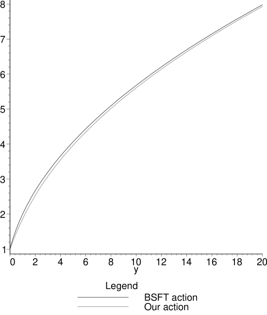
Figure 1: The kinetic terms, i.e. ${\cal{L}}$ as a function of $y=\partial_{m}T\partial^{m}T$ at $T=0$ found in BSFT (18) and in our action (2.3).

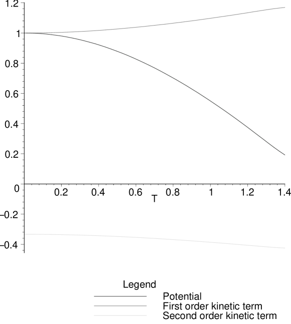
Figure 2: The potential and coefficients of the $\kappa^{\prime}\partial_{m}T\partial^{m}T$ $(\kappa^{\prime}\partial_{m}T\partial^{m}T)^{2}$ terms obtained in section three.

References

- [1] O. Bergman and M. R. Gaberdiel, Nucl. Phys. B499 (1997) 183, hep-th/9701137.
- [2] J. D. Blum and K. R. Dienes, Phys. Lett. B414 (1997) 260, hep-th/9707148.
- [3] J. D. Blum and K. R. Dienes, Nucl. Phys. B516 (1998) 83, hep-th/9707160.
- [4] A. Sen, JHEP 06 (1998) 007, hep-th/9803194.
- [5] A. Sen, JHEP 08 (1998) 020, hep-th/9805019.
- [6] O. Bergman and M.R. Gaberdiel, Phys. Lett. B441 (1998) 133, hep-th/9806155.
- [7] J. A. Harvey, Phys. Rev. D59 (1999) 026002, hep-th/9807213.
- [8] S. Kachru and E. Silverstein, JHEP 11 (1998) 001, hep-th/9808056.
- [9] A. Sen, JHEP 09 (1998) 023, hep-th/9808141.
- [10] A. Sen, JHEP 10 (1998) 021, hep-th/9809111.
- [11] E. Witten, JHEP 12 (1998) 019, hep-th/9810188.
- [12] A. Sen, JHEP 12 (1998) 021, hep-th/9812031.
- [13] I. Sachs, JHEP 11 (1999) 011, hep-th/9907201.
- [14] O. Bergman and M.R. Gaberdiel, JHEP 03 (1999) 013, hep-th/9901014.
- [15] G. Aldazabal and A. M. Uranga, JHEP 10 (1999) 024, hep-th/9908072.
- [16] G. Aldazabal, L.E.Ibanez and F. Quevedo, JHEP 01 (2000) 031, hep-th/9909172.
- [17] T. Dasgupta and B. Stefanski Jr, Nucl. Phys. B572 (2000) 95, hep-th/9910217.
- [18] C. Angelantonj, I. Antoniadis, G. D’Appollonio, E. Dudas and A. Sagnotti, Nucl. Phys. B572 (2000) 36, hep-th/9911081.
- [19] S. Kachru and E. Silverstein, Phys. Rev. Lett. 80 (1998) 4855, hep-th/9802183.
- [20] I. R. Klebanov and A. A. Tseytlin, Nucl. Phys. B546 (1999) 155 , hep-th/9811035.
- [21] I. R. Klebanov and A. A. Tseytlin, Nucl. Phys. B547 (1999) 143, hep-th/9812089.
- [22] I. Antoniadis, E. Dudas and A. Sagnotti, Phys. Lett. B464 (1999) 38, hep-th/9908023.
- [23] N.D. Lambert and I. Sachs, JHEP 05 (2000) 200, hep-th/0002061.
- [24] N.D. Lambert and I. Sachs, JHEP 08 (2000) 024, hep-th/0006122.
- [25] N.D. Lambert and I. Sachs, hep-th/0009155.
- [26] N.D. Lambert and I. Sachs, JHEP 02 (2001) 018, hep-th/0010045.
- [27] J. Polchinski, Phys. Rev. Lett. 75 (1995) 4724, hep-th/9510017.
- [28] T.Banks and L.Susskind, hep-th/9511194.
- [29] K. Bardakci, Nucl. Phys. B68 (1974) 331. K. Bardakci and M.B. Halpern, Phys. Rev. D10 (1974) 4230. K. Bardakci and M.B. Halpern, Nucl. Phys. B96 (1975) 285. K.Bardakci, Nucl. Phys. B133 (1978) 297.
- [30] E.S. Fradkin and A.A. Tseytlin, Phys. Lett. B163 (1985) 123.
- [31] R. Leigh, Mod. Phys. Lett.A4 (1989) 2767.
- [32] A. Abbouelsaood, C.G. Callan, C.R. Nappi and S.A. Yost, Nucl. Phys B280 (1987) 599.
- [33] J. A. Minahan and B. Zwiebach, JHEP 09 (2000) 029, hep-th/0008231.
- [34] J. A. Minahan and B. Zwiebach, hep-th/0009246.
- [35] J. A. Minahan and B. Zwiebach, JHEP 02 (2001) 034, hep-th/0011226.
- [36] E. Witten, Nucl. Phys. B268 (1986) 253.
- [37] E. Witten, Phys. Rev. D46 (1992) 5467, hep-th/9208027.
- [38] S. L. Shatashvili, Phys. Lett. B311 (1993) 83, hep-th/9303143.
- [39] S. L. Shatashvili, hep-th/9311177.
- [40] A. Sen, JHEP 08 (1998) 012, hep-th/9805170.
- [41] V.A. Kostelecky and S. Samuel, Nucl. Phys. B336 (1990) 263.
- [42] A. Sen, JHEP 12 (1998) 027, hep-th/9911116.
- [43] A. Sen and B. Zwiebach, JHEP 03 (2000) 002, hep-th/9912249.
- [44] J. A. Harvey and P. Kraus, JHEP 04 (2000) 012, hep-th/0002117.
- [45] N. Moeller and W. Taylor, Nucl. Phys. B583 (2000) 105, hep-th/0002237.
- [46] R. de Mello Koch, A. Jevicki, M. Mihailescu and R. Tatar, Phys. Lett. B482 (2000) 249, hep-th/0003031.
- [47] P-J. De Smet and J. Raeymaekers, JHEP 05 (2000) 051, hep-th/0003220.
- [48] A. Iqbal and A. Naqvi, JHEP 01 (2001) 040, hep-th/0004015.
- [49] N. Moeller, A. Sen and B. Zwiebach, JHEP 08 (2000) 039, hep-th/0005036.
- [50] E. Witten, Phys. Rev. D47 (1993) 3405, hep-th/9210065.
- [51] J. A. Harvey, D. Kutasov and E. J. Martinec, hep-th/0003101.
- [52] A. A. Gerasimov and S. L. Shatashvili, JHEP 10 (2000) 034, hep-th/0009103.
- [53] D. Kutasov, M. Marino and G. Moore, JHEP 10 (2000) 045, hep-th/0009148.
- [54] D. Kutasov, M. Marino and G. Moore, hep-th/0010108.
- [55] O. Andreev, hep-th/0104061.
- [56] A. A. Gerasimov and S. L. Shatashvili, JHEP 01 (2001) 019, hep-th/0011009.
- [57] A. A. Tseytlin, hep-th/0011033.
- [58] S. Dasgupta and T. Dasgupta, hep-th/0010247.
- [59] P. Kraus and F. Larsen, hep-th/0012198.
- [60] T. Takayanagi, S. Terashima and T. Uesugi, JHEP 03 (2001) 019, hep-th/0012210.
- [61] G. Arutyunov, S. Frolov, S. Theisen and A.A. Tseytlin, JHEP 02 (2001) 002, hep-th/0012080.
- [62] M.R. Garousi, Nucl. Phys. B584 (2000) 284, hep-th/0003122.
- [63] E.A. Bergshoeff, M. de Roo, T.C. de Wit, E. Eyras and S. Panda, JHEP 05 (2000) 009, hep-th/0003221.