Wilsonian Renormalization Group
and the Non-Commutative IR/UV Connection

Abstract:

We study the IR/UV connection of the four-dimensional non-commutative $\phi^{4}$ theory by using the Wilsonian Renormalization Group equation. Extending the usual formulation to the non-commutative case we are able to prove UV renormalizability to all orders in perturbation theory. The full RG equations are finite in the IR, but perturbative approximations of them are plagued by IR divergences. The latter can be systematically resummed in a way analogous to what is done in finite temperature field theory. As an application, next-to-leading order corrections to the two-point function are explicitly computed. The usual Wilsonian picture, i.e. the insensitivity of the IR regime to the UV, does not hold in the non-commutative case. Nevertheless it can be partially recovered by a matching procedure, in which a high-energy theory, defined in the deep non-commutative regime, is connected at some intermediate scale to a commutative low-energy theory. The latter knows about non-commutativity only through the boundary conditions for two would-be irrelevant couplings.

1 Introduction

Recently a lot of interest has been devoted to the study of quantum field theories on non-commutative spaces. The main motivation arises directly from their tight relation with string theories: low energy excitations of a $D$-brane in a magnetic $B_{\mu\nu}$ background are indeed described by field theories with space non-commutativity [1]. In this limit the relevant description of dynamics is in terms of massless open string states, while massive open string states and closed strings decouple: the full consistent string theory seems therefore truncated to the usual field theoretical degrees of freedom. Explicit computations have been performed in [2], showing that the robustness of the above picture holds even after string loop effects are included: this strongly suggests the possibility that the related quantum field theories are well defined too. On the other hand the consistency of the latter is far from being obvious when examined from a purely field theoretical point of view: they are non-local (involving an arbitrarily high number of derivatives in the couplings) and there is a new dimensional parameter, other than the masses, taking into account the scale at which non-commutativity becomes relevant. In particular, unitarity and renormalizability may be in jeopardy: it was shown in fact in [3, 4] that when the non-commutativity involves space and time the perturbative unitarity is in trouble, while in the pure spatial case consistency with the Cutkoski’s rules and positivity properties has been checked [3, 4]. While these results could be expected from string theory – as massive string states do not decouple in the case of space-time non-commutativity [5] – the issue of renormalizability is more subtle. Contrary to early suggestions it was in fact found [6] that infinities appear when perturbative computations are performed in non-commutative scalar theories, the extension of this result to fermionic, gauge and supersymmetric theories being straightforward. The non-local character of the theory could therefore invalidate the usual proofs of renormalizability, which are based on the polynomial nature of the divergent terms in perturbation theory. Moreover, an highly non-trivial mixture between ultraviolet (UV) and infrared (IR) phenomena was observed first in scalar theories [7] and then in gauge theories [8]: this property, being probably the most surprising feature of non-commutative quantum field theories, is known as the IR/UV mixing. It happens that some UV divergences are regulated by an effective cut-off $O(M_{NC}^{2}/p)$, where $M_{NC}$ is the typical scale induced by non-commutativity and $p$ a typical external momentum. Then, as $p\to 0$, a singular IR behavior appears in the perturbative results, even for massive theories, which is actually the remnant of UV divergences of the corresponding commutative theory. If $\Lambda_{0}$ is the overall UV cut-off, it is easy to show that the limit $p\to 0$ does not commute with $\Lambda_{0}\to\infty$, suggesting a dangerous dependence of infrared physics from very high-energy modes. The basis of the program of renormalization seems therefore in trouble and doubts have been casted on the predictivity of the theory itself. Moreover, the IR behavior becomes extremely problematic when the IR/UV terms appear as subdiagrams at higher orders. For instance, in the massless theory the would-be one-loop UV divergence, regulated by the non-commutativity, finds a new avatar as a two-loop IR divergence, independently of the scale of the external momenta.

Concerning the UV behavior, the only four-dimensional theory that has been proved to be renormalizable at any loop order is the Wess-Zumino model [9]. Actually, supersymmetric theories are easier to investigate because the IR/UV mixing generates only logarithmic divergences in the external momenta [8] (this is related to the absence of quadratic divergences in their commutative counterpart). Investigations of non-commutative supersymmetric Yang-Mills were presented in [10]. No general result in this sense has been available up to now for scalar or gauge theories beyond two-loops, mostly due to the extreme complexity of the non-commutative diagrammatics when higher orders are involved. Even in the simple case of the (non-commutative) $\phi^{4}$ theory convergence theorems and recursive subtractions fail to give a definitive answer to the question [11], although renormalizability has been argued since the original quantum investigation [7]. Explicit two-loop computations have been performed in the massive case, showing that the theory can be effectively renormalized at this order: at the same time it was noticed that at higher loops problems arise, due to divergences induced by the presence of the above mentioned IR/UV terms [12]. Non supersymmetric gauge theories have been discussed so far at one-loop [13]. Actually, in ref. [14] it has been claimed that non-commutative QED is renormalizable at all orders. However, that paper is based on mapping the non-commutative gauge theory on a commutative one, where the IR/UV problem is absent. The connection between this approach and the usual diagrammatic one is not clear.

The purpose of this paper is to study the IR/UV connection of the non-commutative $\phi^{4}$ theory using the Wilsonian Renormalization Group equation (RG) [15], as formulated by Polchinski [16] in the case of quantum field theories. The RG turns out to be a very powerful tool in order to disentangle the IR side of the problem from the UV one. The main feature that we will use is the introduction of an explicit momentum cut-off, $\Lambda$, which can take any value between the UV cut-off, $\Lambda_{0}$, and zero. The RG equations describe the evolution of the couplings of the theory as loops with momenta between $\Lambda_{0}$ and $\Lambda$ are included, with $\Lambda$ eventually going to the physical value $\Lambda\to 0$. A two-steps strategy is then possible. First, take $\Lambda$ much larger than any physical mass scale (but $\Lambda\ll\Lambda_{0}$) and sample the UV sector of the theory, discussing under which conditions the $\Lambda_{0}\to\infty$ limit can be taken (UV renormalizability). Second, study the IR limit by sending $\Lambda\to 0$ (IR finiteness).

Besides the neat separation between UV and IR, there is another feature of the RG which will be of great use in the following. The RG equations are formally one-loop equations in which the tree-level vertices and propagators are replaced by full– $\Lambda$-dependent– ones. Thus, perturbation theory is reproduced by solving the full equations iteratively, putting the $n$-th order propagators and vertices in and getting those at $(n+1)$-th order out upon integration.

The two features above were used in [16] and in [17] to prove perturbative UV renormalizability of the commutative $\phi^{4}$ theory to all orders and, in the massless case, the IR finiteness of the theory [17]. These proofs are extremely simple. They are essentially based on power counting and do not require any analysis of overlapping divergences of Feynman diagrams. As we will see, this holds for the non-commutative case as well.

Our results can be summarized as follows:

• UV renormalization is proved to all orders in perturbation theory;

• the full RG equations are finite in the IR, but perturbative approximations of them are plagued by IR divergences. The latter can be systematically resummed in a way analogous to what is done at finite temperature (Hard Thermal Loop (HTL) resummation [18, 20]). Next-to-leading order corrections to the two-point function are explicitly calculated (see also [21]);

• the usual Wilsonian picture, i.e. the insensitivity of the IR regime to the UV, is lost in the non-commutative case. Nevertheless, it can be partially recovered by a matching procedure, in which a high-energy theory, defined in the deep non-commutative regime, is connected at some intermediate scale to a commutative low-energy theory. The latter knows about high-energy non-commutativity only via the boundary conditions for two would-be irrelevant couplings.

The plan of the paper is the following. In sect. 2 we introduce the non-commutative version of the four-dimensional real $\phi^{4}$ theory, we display the Feynman rules and we discuss the difference between planar and non-planar diagrams in a specific example, the two-point function. The IR/UV mixing is presented by a one-loop computation and the problems arising when higher orders are considered are exemplified. In sect. 3 we review the Wilsonian RG approach to UV renormalization and IR finiteness in the commutative case, illustrating the procedure developed in [17]. In sect. 4 we extend the formulation of the RG to the non-commutative case and we prove the UV renormalizability of the theory to all perturbative orders. Then, we discuss the IR regime. We show the necessity of a resummation and perform it by modifying the tree-level propagator and adding a proper counterterm in order to avoid overcounting. As an application, we review our recent calculation of next-to-leading corrections to the two-point function [21]. In sect. 5 we discuss the sensitivity of the theory in the IR regime to the high-energy theory. We point out that UV/IR mixing destroys the usual Wilsonian picture and discuss how it can be partially recovered by a suitable matching procedure. Finally, in sect. 6 we summarize our results and discuss some possible implications of them.

2 Non-commutative field theory

Non-commutative spaces are defined by the following generalization of the usual quantum commutation relations

$$[\hat{x}^{\mu},\hat{x}^{\nu}]=i\Theta^{\mu\nu}\,,\,\,\,\,\,\,[\hat{x}_{i},\hat{p}_{j}]=i\delta_{ij}\,,$$ (1)

where $\Theta^{\mu\nu}$ is a constant anti-symmetric matrix of dimension $[M]^{-2}$, greek indices run from zero to three and latin ones from one to three. It was shown in ref. [3, 4] that when any $\Theta^{0i}$ is different from zero perturbative unitarity is in trouble, so that in order to get a consistent field theory one should consider only spatial indices also in the first of eqs. (1). Since we will work in Euclidean space, we will ignore the problem and consider a generic $\Theta$-matrix.

A non-zero $\Theta^{\mu\nu}$ breaks Lorentz invariance, therefore explicit dependence on $\tilde{p}^{\mu}\equiv\Theta^{\mu\nu}p^{\nu}$, with $p^{\nu}$ a generic external momentum, is to be expected on general grounds.

In order to construct a field theory, it is convenient to use the so-called Weyl-Moyal correspondence which amounts to work on the usual commutative space while redefining the multiplication between functions according to

$$f_{1}(x)f_{2}(x)\rightarrow(f_{1}\star f_{2})(x)\equiv\left.e^{\frac{i}{2}\Theta^{\mu\nu}\partial^{y}_{\mu}\partial^{z}_{\nu}}f_{1}(y)f_{2}(z)\right|_{y=z=x}\,.$$ (2)

It is easy to check that the Moyal bracket between the commuting $x_{\mu}$ and $x_{\nu}$ consistently replaces the relations in (1), that is

$$[x^{\mu},x^{\nu}]_{MB}=x^{\mu}\star x^{\nu}-x^{\nu}\star x^{\mu}=i\Theta^{\mu\nu}\,.$$

The action for the Euclidean real scalar theory becomes

$$S[\phi]=\frac{1}{2}\displaystyle\int\frac{d^{4}p}{(2\pi)^{4}}\left[\phi(p)(p^{2}+m^{2})\phi(-p)\right]$$

$$\displaystyle+\frac{g^{2}}{4!}\int\left(\prod_{a=1}^{4}\frac{d^{4}p_{a}}{(2\pi)^{4}}\phi(p_{a})\right)(2\pi)^{4}\delta^{(4)}\left(\sum_{a=1}^{4}p_{a}\right)e^{ip_{12}}e^{ip_{34}}\,,$$ (3)

where

$$p_{ab}\equiv\frac{p_{a}\cdot\tilde{p}_{b}}{2}\;.$$

As we see, the quadratic part is the same as in the commutative case, due to the antisymmetry of $\Theta^{\mu\nu}$, so the propagator is still $D(p)=(p^{2}+m^{2})^{-1}$, while the Feynman rule for the interaction vertex gets modified according to

$$\Gamma^{(4)}(p_{1},p_{2},p_{3},p_{4})=g^{2}h(p_{1},p_{2},p_{3},p_{4})$$

$$\equiv\frac{g^{2}}{3}\left[\cos(p_{12})\cos(p_{34})+\cos(p_{13})\cos(p_{24})+\cos(p_{14})\cos(p_{23})\right]\,.$$ (4)

The Moyal phase factor modifies the behavior of loop integrals with respect to the commutative case. Consider the one-loop correction to the self-energy

$$\Sigma_{\Lambda_{0}}(p) =-\displaystyle\frac{g^{2}}{6}\int\frac{d^{4}q}{(2\pi)^{4}}\Theta(\Lambda_{0}^{2}-q^{2})\frac{1}{q^{2}+m^{2}}\left[2+\cos(q\cdot\tilde{p})\right]$$ (5)

$$=-\frac{g^{2}}{32\pi^{2}}\left[\frac{2}{3}\Lambda_{0}^{2}+\frac{4}{3~{}\tilde{p}^{2}}\left(1-J_{0}(\Lambda_{0}~{}\tilde{p})\right)\right]\;,\;\;\;(m^{2}\ll\mathrm{min}\{\Lambda_{0}^{2},1/\tilde{p}^{2}\})$$

where we have regulated the UV quadratic divergences by means of a momentum cut-off. The first term in parenthesis exhibits the usual $\Lambda_{0}^{2}$ behavior of the commutative case with a coefficient $2/3$ instead of $1$. This is the contribution of the so-called ‘planar’ graphs, in which two nearby scalar legs are contracted in order to get the tadpole loop. The second term comes from the non-planar graphs and contains a non-vanishing phase factor. It exhibits the two limiting behaviors

$$\displaystyle\frac{4}{3~{}\tilde{p}^{2}}\left(1-J_{0}(\Lambda_{0}~{}\tilde{p})\right) \to\frac{1}{3}\Lambda_{0}^{2}\;\;\;\;\;\;\;\;\;({\mathrm{a}s}~{}\Lambda_{0}~{}\tilde{p}\to 0)$$ (6)

$$\to\frac{4}{3}\frac{1}{\tilde{p}^{2}}\;\;\;\;\;\;\;\;\;({\mathrm{a}s}~{}\Lambda_{0}~{}\tilde{p}\to\infty)\;,$$

from which we see that if we take the commutative limit $\Theta^{\mu\nu}\to 0$ before removing the cut-off, the ‘missing’ UV divergence $\Lambda_{0}^{2}/3$ is recovered. On the other hand, if we let $\Lambda_{0}\to\infty$ first, the oscillating term provides an effective UV cut-off $2/|\tilde{p}|$, which regulates the integral leaving a $\Lambda_{0}$-independent term. Thus, in the non-commutative theory we generally have:

• different coefficients for the UV divergent terms;

• new IR-dangerous terms, induced by the effective UV cut-off, $2/|\tilde{p}|$.

It is rather clear that when we insert the tadpole (5) in higher order contributions to the self-energy, we get more and more IR divergent integrals (we present only the leading contribution to the singularity at a given order)

$$g^{2}\int\frac{d^{4}q}{(2\pi)^{4}}\frac{1}{(q^{2}+m^{2})^{n+1}}\Sigma(q)^{n}\to g^{2n+2}\int\frac{d^{4}q}{(2\pi)^{4}}\frac{1}{(q^{2}+m^{2})^{n+1}}\frac{1}{\tilde{q}^{2n}}\;\;\;\;(\mathrm{IR})\;,$$ (7)

which make the self-energy IR divergent at $O(g^{4})$ in the massless ($m=0$) case and at $O(g^{6})$ in the massive one.

The connection between the UV and IR divergences that we have just outlined makes a proof of perturbative renormalizability along the usual lines quite cumbersome. The main difficulty lies manifestly in the difficulty in disentangling the UV from the IR sectors of the loop integrals. Indeed, the possibility of absorbing UV divergences by means of local counterterms has been discussed at two-loop in refs. [11, 12, 22], but no finite result could be obtained at that order, in the massless theory, due to the pathological behavior of the integrals in the IR. Although this difficulty was recognized since the original work on the subject [7], no proposal has been done up to now to systematically handle these divergences and no results have been presented by taking consistently into account higher orders.

In the following we will show that the use of Wilsonian methods, where an explicit momentum cut-off separates the IR from the UV, is of great help in organizing a perturbative proof of renormalizability. At the same time, the structure of the exact RG equations suggests an appropriate procedure to tame IR singularities.

3 Wilsonian RG in the commutative case

In this section we review the formulation of the RG à la Polchinski [16] in the commutative theory. Following ref. [17], we will review the use of the RG to demonstrate perturbative renormalizability of the real scalar theory and IR finiteness in the massless case.

3.1 The Wilsonian flow

Our starting point is the path integral

$$\displaystyle Z[J]=e^{W[J]}=\int{\cal D}\phi\>\> \exp\left\{-\frac{1}{2}\int\frac{d^{4}p}{(2\pi)^{4}}\phi(p)D^{-1}\phi(-p)-S_{\mathrm{i}nt}[\phi]\right.$$ (8)

$$\>\>\>\>\>\displaystyle+\left.\int\frac{d^{4}p}{(2\pi)^{4}}\phi(p)J(-p)\right\}\;,$$

where the interaction action $S_{\mathrm{i}nt}[\phi]$ contains the bare couplings and has a $Z_{2}$ $\phi\to-\phi$ symmetry. We now introduce an UV cut-off, $\Lambda_{0}$, and a IR one, $\Lambda$, by making the substitution

$$D(p)\rightarrow D_{\Lambda,\Lambda_{0}}(p)\equiv D(p)K_{\Lambda,\Lambda_{0}}(p)$$

in eq. (8), where $K_{\Lambda,\Lambda_{0}}(p)$ is equal to one for $\Lambda^{2}<p^{2}<\Lambda_{0}^{2}$ and vanishes rapidly outside. The substitution above defines $Z_{\Lambda,\Lambda_{0}}$ and $W_{\Lambda,\Lambda_{0}}$, the generating functionals of Green functions in which only momenta between $\Lambda$ and $\Lambda_{0}$ have been integrated out. By differentiating w.r.t $\Lambda$ we get the RG equation for $Z_{\Lambda,\Lambda_{0}}$

$$\Lambda\frac{\partial\;\;}{\partial\Lambda}Z_{\Lambda,\Lambda_{0}}[J]=-\mbox{\small$\frac{1}{2}$}\int\frac{d^{4}q}{(2\pi)^{4}}\Lambda\frac{\partial\;\;}{\partial\Lambda}D_{\Lambda,\Lambda_{0}}^{-1}(q)(2\pi)^{8}\frac{\delta^{2}Z_{\Lambda,\Lambda_{0}}[J]}{\delta J(q)\delta J(-q)}\;.$$ (9)

In order to discuss the issue of renormalizability, it is more convenient to consider the 1PI generating functional, defined as usual as

$$\Gamma_{\Lambda,\Lambda_{0}}[\phi]=-W_{\Lambda,\Lambda_{0}}[J]+W_{\Lambda,\Lambda_{0}}[0]+\int\frac{d^{4}p}{(2\pi)^{4}}\phi(p)J(-p)\;,$$ (10)

where $\displaystyle\phi(p)=\frac{1}{(2\pi)^{4}}\frac{\delta W_{\Lambda,\Lambda_{0}}[J]}{\delta J(-p)}$.

Cut-off, 1PI, 2n-point functions are then given by

$$(2\pi)^{4}\delta^{(4)}(\sum_{i}p_{i})\Gamma^{2n}_{\Lambda,\Lambda_{0}}(p_{1},\ldots,p_{2n})=(2\pi)^{8}\frac{\delta^{2n}\Gamma_{\Lambda,\Lambda_{0}}[J]}{\delta\phi(p_{1})\cdots\delta\phi(p_{2n})}\;.$$ (11)

From the definitions above and from the RG equation (9) we get the evolution equations for the 1PI Green functions [17]. Isolating the interacting part of the two-point function,

$$\Gamma^{2}_{\Lambda,\Lambda_{0}}(p)=D^{-1}_{\Lambda,\Lambda_{0}}(p)+\Sigma_{\Lambda,\Lambda_{0}}(p)\;,$$ (12)

we have

$$\Lambda\frac{\partial\;\;}{\partial\Lambda}\Sigma_{\Lambda,\Lambda_{0}}(p)=\mbox{\small$\frac{1}{2}$}\int\frac{d^{4}q}{(2\pi)^{4}}\frac{S_{\Lambda,\Lambda_{0}}(q)}{q^{2}+m^{2}}\Gamma^{4}_{\Lambda,\Lambda_{0}}(q,p,-p,-q)\;,$$ (13)

while for $n\geq 2$ we have

$$\Lambda\frac{\partial\;\;}{\partial\Lambda}\Gamma^{2n}_{\Lambda,\Lambda_{0}}(p_{1},\ldots,p_{2n})=\mbox{\small$\frac{1}{2}$}\int\frac{d^{4}q}{(2\pi)^{4}}\frac{S_{\Lambda,\Lambda_{0}}(q)}{q^{2}+m^{2}}\overline{\Gamma}^{2n+2}_{\Lambda,\Lambda_{0}}(q,p_{1},\ldots,p_{2n},-q)\;,$$ (14)

with

$$\overline{\Gamma}^{2n+2}_{\Lambda,\Lambda_{0}}(q,p_{1},\ldots,p_{2n},q^{\prime})=\Gamma^{2n+2}_{\Lambda,\Lambda_{0}}(q,p_{1},\ldots,p_{2n},q^{\prime})-$$

$$\sum_{k=1}^{n-1}\Gamma^{2k+2}_{\Lambda,\Lambda_{0}}(q,p_{i_{1}},\ldots,p_{i_{2k}},-Q)\frac{1}{\Gamma^{2}_{\Lambda,\Lambda_{0}}(Q)}\overline{\Gamma}^{2n-2k+2}_{\Lambda,\Lambda_{0}}(Q,p_{i_{2k+1}},\ldots,p_{i_{2n}},q^{\prime})\;.$$ (15)

The kernel in eqs. (13,14) is given by

$$\displaystyle\frac{S_{\Lambda,\Lambda_{0}}(q)}{q^{2}+m^{2}} \displaystyle\equiv\Lambda\frac{\partial\;\;}{\partial\Lambda}\left.\frac{1}{(q^{2}+m^{2})K_{\Lambda,\Lambda_{0}}(q)^{-1}+\Sigma_{\Lambda^{\prime},\Lambda_{0}}(q)}\right|_{\Lambda^{\prime}=\Lambda}\,,$$ (16)

$$\displaystyle=\frac{1}{q^{2}+m^{2}}\frac{1}{\left[1+\frac{\Sigma_{\Lambda,\Lambda_{0}}(q)}{q^{2}+m^{2}}K_{\Lambda,\Lambda_{0}}(q)\right]^{2}}\Lambda\frac{\partial\;\;}{\partial\Lambda}K_{\Lambda,\Lambda_{0}}(q)\;.$$

There is a simple recipe for deriving the RG equation for a given Green function:

• write the one-loop expression for $\Gamma^{(2n)}$ obtained by using all the vertices up to $\Gamma^{(2n+2)}$, as if they were formally tree-level;

• promote the tree-level vertices above to full, running, vertices, $\Gamma^{(2n)}\rightarrow\Gamma_{\Lambda,\Lambda_{0}}^{(2n)}$, and the tree-level propagator to the full, cut-off, propagator;

• take the derivative with respect to $\Lambda$ everywhere in the $K$’s but not in the $\Sigma$’s or $\Gamma$’s.

The fact that the RG equations are formally one-loop is crucial in allowing a iterative proof of perturbative renormalizability, as we review in the following subsection.

3.2 RG flows for relevant and irrelevant couplings

We now impose the renormalization conditions

$$\Gamma_{2}(p^{2}=p_{0}^{2})=m^{2}+p_{0}^{2},\;\;\;\;\;\left.\frac{d\Gamma_{2}(p^{2})}{dp^{2}}\right|_{p^{2}=p_{0}^{2}}=1,\;\;\;\;\;\Gamma_{4}(\bar{p}_{1},\ldots,\bar{p}_{4})=g^{2}\;,$$ (17)

with the symmetric renormalization point defined as $\bar{p}_{i}\cdot\bar{p}_{j}=p_{0}^{2}(\delta_{ij}-\frac{1}{4})$. In order to study UV renormalization, the ‘relevant’ operators, i.e. those with non-negative mass dimension, have to be isolated. They are

$$\gamma_{2}(\Lambda)\equiv\left.\frac{d\Sigma_{\Lambda,\Lambda_{0}}(p)}{dp^{2}}\right|_{p^{2}=p_{0}^{2}},\;\;\;\;\gamma_{3}(\Lambda)\equiv\left.\Sigma_{\Lambda,\Lambda_{0}}(p)\right|_{p^{2}=p_{0}^{2}},\;\;\;\;\gamma_{4}(\Lambda)\equiv\Gamma^{4}_{\Lambda,\Lambda_{0}}(\bar{p}_{1},\ldots,\bar{p}_{4})\,.$$ (18)

The two– and four–point functions can be rewritten as

$$\displaystyle\Sigma_{\Lambda,\Lambda_{0}}(p)=\gamma_{3}(\Lambda)+(p^{2}-p_{0}^{2})\gamma_{2}(\Lambda)+\Delta^{2}_{\Lambda,\Lambda_{0}}(p)$$

$$\displaystyle\Gamma^{4}_{\Lambda,\Lambda_{0}}(p_{1},\ldots,p_{4})=\gamma_{4}(\Lambda)+\Delta^{4}_{\Lambda,\Lambda_{0}}(p_{1},\ldots,p_{4})$$ (19)

where $\Delta^{2}$ and $\Delta^{4}$ satisfy $\Delta^{2}_{\Lambda,\Lambda_{0}}(p^{2}=p_{0}^{2})=0$, $\Delta^{4}_{\Lambda,\Lambda_{0}}(\bar{p}_{1},\ldots,\bar{p}_{4})=0$. They are ‘irrelevant’ operators together with all $\Gamma^{2n}_{\Lambda,\Lambda_{0}}$’s with $n>2$. The RG equations for relevant and irrelevant operators can be read from eqs. (13), (14), and form a system of coupled differential equations giving the evolution of the couplings as the IR cut-off $\Lambda$ is lowered from $\Lambda=\Lambda_{0}$ to $\Lambda=0$. The renormalization conditions corresponding to eq. (17) are imposed by fixing the boundary conditions for the relevant couplings at the physical point $\Lambda=0$:

$$\gamma_{2}(0)=0,\,\,\,\gamma_{3}(0)=0,\,\,\,\gamma_{4}(0)=g^{2}\;.$$ (20)

The irrelevant couplings are fixed at the UV point $\Lambda_{0}$, where they can be taken to be vanishing

$$\Delta^{2}_{\Lambda_{0},\Lambda_{0}}(p)=\Delta^{4}_{\Lambda_{0},\Lambda_{0}}(p_{1},\ldots,p_{4})=\Gamma^{2n}_{\Lambda_{0},\Lambda_{0}}(p_{1},\ldots,p_{2n})=0\;\;\;\;\;\;\;\;\;\;\;(n>2)\;.$$ (21)

Integrating the RG equations with the above boundary conditions leads to a set of coupled integral equations

$$\gamma_{2}(\Lambda) = \displaystyle\mbox{\small$\frac{1}{2}$}\int\frac{d^{4}q}{(2\pi)^{4}}\int_{0}^{\Lambda}\frac{d\lambda}{\lambda}\frac{S_{\lambda,\Lambda_{0}}(q)}{q^{2}+m^{2}}\left.\frac{\partial\;\;}{\partial p^{2}}\Gamma^{4}_{\lambda,\Lambda_{0}}(q,p,-p,-q)\right|_{p^{2}=p_{0}^{2}}\;,$$

$$\gamma_{3}(\Lambda) = \displaystyle\mbox{\small$\frac{1}{2}$}\int\frac{d^{4}q}{(2\pi)^{4}}\int_{0}^{\Lambda}\frac{d\lambda}{\lambda}\frac{S_{\lambda,\Lambda_{0}}(q)}{q^{2}+m^{2}}\left.\Gamma^{4}_{\lambda,\Lambda_{0}}(q,p,-p,-q)\right|_{p^{2}=p_{0}^{2}}\;,$$

$$\gamma_{4}(\Lambda) = \displaystyle g^{2}+\mbox{\small$\frac{1}{2}$}\int\frac{d^{4}q}{(2\pi)^{4}}\int_{0}^{\Lambda}\frac{d\lambda}{\lambda}\frac{S_{\lambda,\Lambda_{0}}(q)}{q^{2}+m^{2}}\;\overline{\Gamma}^{6}_{\lambda,\Lambda_{0}}(q,\bar{p}_{1},\ldots,\bar{p}_{4},-q)\;,$$ (22)

for the relevant couplings, and

$$\Delta^{2}_{\Lambda,\Lambda_{0}}(p)=\displaystyle-\mbox{\small$\frac{1}{2}$}\int\frac{d^{4}q}{(2\pi)^{4}}\int_{\Lambda}^{\Lambda_{0}}\frac{d\lambda}{\lambda}\frac{S_{\lambda,\Lambda_{0}}(q)}{q^{2}+m^{2}}\Delta\Gamma^{4}_{\lambda,\Lambda_{0}}(q,p,-p,-q)\;,$$

$$\Delta^{4}_{\Lambda,\Lambda_{0}}(p_{1},\ldots,p_{4})=\displaystyle-\mbox{\small$\frac{1}{2}$}\int\frac{d^{4}q}{(2\pi)^{4}}\int_{\Lambda}^{\Lambda_{0}}\frac{d\lambda}{\lambda}\frac{S_{\lambda,\Lambda_{0}}(q)}{q^{2}+m^{2}}\Delta\overline{\Gamma}^{6}_{\lambda,\Lambda_{0}}(q,p_{1},\ldots,p_{4},-q)\;,$$

$$\displaystyle\Gamma^{2n}_{\Lambda,\Lambda_{0}}(p_{1},\ldots,p_{2n})=-\mbox{\small$\frac{1}{2}$}\int\displaystyle\frac{d^{4}q}{(2\pi)^{4}}\int_{\Lambda}^{\Lambda_{0}}\frac{d\lambda}{\lambda}\frac{S_{\lambda,\Lambda_{0}}(q)}{q^{2}+m^{2}}\;\overline{\Gamma}^{2n+2}_{\lambda,\Lambda_{0}}(q,\bar{p}_{1},\ldots,\bar{p}_{2n},-q)\;,\;\;\;\;(n>2)$$

where

$$\Delta\Gamma^{4}_{\lambda,\Lambda_{0}}(q,p,-p,-q)\equiv\Gamma^{4}_{\lambda,\Lambda_{0}}(q,p,-p,-q)-\left.\Gamma^{4}_{\lambda,\Lambda_{0}}(q,p,-p,-q)\right|_{p^{2}=p_{0}^{2}}$$

$$\;\;\;\;\;\;\;\;\;\;\;\;\;\;\;\;\;\;\;\;\;\;\;\;\;\;\;\;\;\;\;\;\;\;\;\;\displaystyle-(p^{2}-p_{0}^{2})\left.\frac{\partial\;\;}{\partial p^{2}}\Gamma^{4}_{\lambda,\Lambda_{0}}(q,p,-p,-q)\right|_{p^{2}=p_{0}^{2}}\;,$$

$$\Delta\overline{\Gamma}^{6}_{\lambda,\Lambda_{0}}(q,p_{1},\ldots,p_{4},-q)\equiv\overline{\Gamma}^{6}_{\lambda,\Lambda_{0}}(q,p_{1},\ldots,p_{4},-q)-\overline{\Gamma}^{6}_{\lambda,\Lambda_{0}}(q,\bar{p}_{1},\ldots,\bar{p}_{4},-q)\;.$$

The first aspect to notice about the above equations is the different role played by the cut-off $\Lambda$ for the relevant and the irrelevant operators. In the former case, it acts as a UV cut-off (eq. (3.2)), thus ensuring– by construction– the finiteness of the integrals when the UV cut-off $\Lambda_{0}$ is removed. For the irrelevant couplings $\Lambda$ acts instead as a IR cut-off. The proof of UV renormalizability then amounts to show that in the $\Lambda_{0}\to\infty$ limit the integrals in eq. (3.2) are finite, which is ensured by dimensional reasons and by the subtractions in eq. (3.2). Moreover, in this framework, the discussion of the behavior in the IR is disentangled by that in the UV, as we can take the two limits $\Lambda_{0}\to\infty$ and $\Lambda\to 0$ at different stages. This will turn out to provide useful insights to the IR/UV connection in the non-commutative theory.

The second relevant aspect of eqs. (3.2,3.2) is that they are formally one-loop integrals with loop momentum $q^{2}\sim\lambda^{2}$. Thus, perturbation theory can be reconstructed from the RG equations by putting the $l$-loop result on the RHS of eqs. (3.2,3.2) and getting the $l+1$-loop result upon integration on $\lambda$.

From now on we will use a sharp momentum IR cut-off, i.e. the kernel $K_{\Lambda,\Lambda_{0}}(q)$ of eq. (16) will contain a Heaviside function $\Theta(\sqrt{q^{2}}-\Lambda)$. Our conclusions on renormalizability and IR finiteness do not rely on the type of cut-off function, but we must specify it in order to get explicit results for $\Lambda\neq 0$ and at any finite order in the approximations. Moreover, the explicit form of the UV cut-off needs not to be specified. The kernel (16) then reads

$$\frac{S_{\Lambda,\Lambda_{0}(q)}}{q^{2}+m^{2}}=-\frac{\Lambda}{\Lambda^{2}+m^{2}}\delta(\Lambda-\sqrt{q^{2}})s(\Lambda)\,,\;\;\;\;\;\;s(\Lambda)=\left(1+\frac{\Sigma_{\Lambda,\Lambda_{0}}(\Lambda)}{\Lambda^{2}+m^{2}}\right)^{-2}\,,$$ (25)

where the two-point function $\Sigma_{\Lambda,\Lambda_{0}}(q)$ is evaluated at $q=\Lambda$, a fact which will turn out to be crucial in the following.

3.3 Proof of UV renormalizability

In order to simplify the power-counting, we take $\Lambda$ much larger than any physical scale in the theory, i.e. $p_{0},m\ll\Lambda\ll\Lambda_{0}$. In this limit the one-loop contributions are given by,

$$\gamma_{2}(\Lambda)=0,\;\;\;\;\;\;\gamma_{3}(\Lambda)=-\frac{g^{2}}{32\pi^{2}}\Lambda^{2},\;\;\;\;\;\gamma_{4}(\Lambda)=\frac{3}{32\pi^{2}}g^{4}\log\frac{\Lambda^{2}}{p_{0}^{2}},\;\;\;\;\;$$

$$\Delta^{2}_{\Lambda,\Lambda_{0}}=0\;\;\;\;\;\Delta^{4}_{\Lambda,\Lambda_{0}}=-\frac{g^{4}}{6\pi^{3}}\frac{\left[\sqrt{(p_{1}+p_{2})^{2}}-\sqrt{(\bar{p}_{1}+\bar{p}_{2})^{2}}\right]+[2\to 3]+[2\to 4]}{\Lambda}\;,$$

$$\Gamma^{2n}_{\Lambda,\Lambda_{0}}=\frac{(-1)^{n+1}(2n)!}{2^{n}n(n-2)32\pi^{2}}\frac{g^{2n}}{\Lambda^{2n-4}},\;\;\;\;(n>2).$$ (26)

The vanishing of $\gamma_{2}$ and $\Delta^{2}$ at one-loop is due to the momentum independence of the tadpole. At two-loop they get non-zero contributions which make them scale as $g^{4}\log\Lambda^{2}$ and $g^{4}(p^{2}-p_{0}^{2})^{2}/\Lambda^{2}$ respectively.

The proof of perturbative UV renormalizability proceeds as follows [17];

• for any function $f^{2n}_{\Lambda,\Lambda_{0}}$ (could be any irrelevant vertex or momentum derivative of it) define

  $$\left|f^{2n}\right|_{\Lambda}\equiv\mathrm{Max}_{p_{i}^{2}<c\Lambda^{2}}\left|f^{2n}_{\Lambda,\Lambda_{0}}(p_{1},\ldots,p_{2n})\right|\;,$$ (27)

  where $c$ is some $O(1)$ numerical constant;

• at $l$-loop assume the following scalings

  $$\gamma_{2}^{(l)}\sim\gamma_{4}^{(l)}\sim\left|\Delta^{4}_{(l)}\right|_{\Lambda}=O(1)\;,\;\;\;\;\gamma_{3}^{(l)}\sim\left|\Delta^{2}_{(l)}\right|_{\Lambda}=O(\Lambda^{2})\;,$$

  $$\left|\partial^{m}\Gamma^{2n}_{(l)}\right|_{\Lambda}\sim\left|\partial^{m}\overline{\Gamma}^{2n}_{(l)}\right|_{\Lambda}=O(\Lambda^{4-2n-m})\;,$$ (28)

  where we have considered only the power-law behavior, since logarithms cannot change the power counting. The scaling behavior of $s_{(l)}(\Lambda)$ can be read from eqs. (25,3.2,ii)),

  $$s_{(l)}(\Lambda)=O(1)\;.$$ (29)

  Notice that none of these behaviors depends on the loop order $l$.

• using eq. (3.2) we can maximize the $l+1$-loop contributions to the irrelevant vertices as follows

  $$\left|\Delta^{2}_{(l+1)}\right|_{\Lambda}\mathrel{\vbox{\hbox{$<$}\nointerlineskip\hbox{$\sim$}}}\Lambda^{4}\int_{\Lambda^{2}}^{\infty}d\lambda^{2}s_{(l-l^{\prime})}(\lambda)\left|\partial^{4}\Gamma^{4}_{(l^{\prime})}\right|_{\lambda}\;,$$ (30)

  $$\left|\Delta^{4}_{(l+1)}\right|_{\Lambda}\mathrel{\vbox{\hbox{$<$}\nointerlineskip\hbox{$\sim$}}}\Lambda^{2}\int_{\Lambda^{2}}^{\infty}d\lambda^{2}s_{(l-l^{\prime})}(\lambda)\left|\partial^{2}\overline{\Gamma}^{6}_{(l^{\prime})}\right|_{\lambda}\;,$$ (31)

  $$\left|\Gamma^{2n}_{(l+1)}\right|_{\Lambda}\mathrel{\vbox{\hbox{$<$}\nointerlineskip\hbox{$\sim$}}}\int_{\Lambda^{2}}^{\infty}d\lambda^{2}s_{(l-l^{\prime})}(\lambda)\left|\overline{\Gamma}^{2n+2}_{(l^{\prime})}\right|_{\lambda}\;,$$ (32)

  where $l^{\prime}=0,\ldots,l$. In deriving (30) and (31) we have used the fact that, due to the subtractions, the vertices of eq. (3.2) scale as

  $$\Delta\Gamma^{4}_{\Lambda,\Lambda_{0}}(q,p,-p,-q)\sim(p^{2}-p_{0}^{2})^{2}\frac{\partial^{4}\;\;}{\partial p^{4}}\Gamma^{4}_{\Lambda,\Lambda_{0}}(q,p,-p,-q)\,,$$

  $$\Delta\overline{\Gamma}^{6}_{\Lambda,\Lambda_{0}}(q,p_{1},\ldots,p_{4},-q)\sim(P^{2}-\bar{P}^{2})\frac{\partial^{2}\;\;}{\partial P^{2}}\overline{\Gamma}^{6}_{\Lambda,\Lambda_{0}}(q,p_{1},\ldots,p_{4},-q)\;,$$

  where $P$ ($\bar{P}$) is a combination of $p_{i}$’s ($\bar{p}_{i}$’s). Thanks to the scaling behaviors in eqs. (ii),29) the $\Lambda_{0}\to\infty$ limit can be taken, as the integrals are dominated by the lower limit $\Lambda$.

• the scalings assumed in eqs. (ii),29) hold at one-loop, see eq. (3.3). By using them in eqs. (30–32), it is now straightforward to check that the same– $l$-independent– behaviors are obtained at $l+1$-loop. UV renormalizability is thus proved by induction at any order.

In summary, the UV cut-off $\Lambda_{0}$ can be removed, provided the three subtractions of eq. (3.2)– corresponding to the three renormalization conditions of eq. (17)– are performed.

3.4 IR finiteness

In the previous subsection the $\Lambda_{0}\to\infty$ limit at fixed– and very large– $\Lambda$ was considered. In the massive– and commutative! – theory the $\Lambda\to 0$ limit can be taken with no particular care as the mass provides an effective IR cut-off regardless of the external momenta.

The massless theory requires a more careful study, which was also performed in [17]. The statement to be proved in this case is the finiteness in the $\Lambda\to 0$ limit of any Green function with no exceptional external momenta, where a couple of external momenta $p_{i}$ and $p_{j}$ is said to be exceptional if $p_{i}+p_{j}=O(\Lambda)$. The proof proceeds again by induction, however it is technically complicated by the fact that the RHS’s of the RG equations involve Green functions with a couple of exceptional momenta $q$ and $-q$. Thus, by iteration, Green functions with any number of pairs of exceptional momenta are involved, and one has to consider the IR behaviors of all these. We do not need here to give all the details, which can be found in [17]. For future comparison with the non-commutative case, we just recall the main feature of the commutative theory allowing IR finiteness being realized order by order in the loop expansion, namely the scaling behavior of the $l$-loop kernel,

$$s_{(l)}(\Lambda)=O((\log\Lambda)^{l-1})\;.$$ (33)

As we will see in sect. 4.2, the mild logarithmic divergence above is turned into a power-law in the non-commutative one, more and more divergent as the loop order increases. As a consequence, any Green function is IR divergent at a sufficiently high order in the perturbative expansion, and the latter has to be properly reorganized in order to obtain finite results.

4 The non-commutative Wilsonian flow

The RG equations (13,14) hold for the non-commutative case as well. In the Wilsonian framework, the non-commutativity of the theory is completely encoded in a different identification of the relevant vertex $\gamma_{4}(\Lambda)$. Indeed, we now write the four-point function as

$$\Gamma^{4}_{\Lambda,\Lambda_{0}}(p_{1},\ldots,p_{4})=h(p_{1},\ldots,p_{4})\left[\gamma_{4}(\Lambda)+\Delta^{4}_{\Lambda,\Lambda_{0}}(p_{1},\ldots,p_{4})\right]\;,$$ (34)

where the oscillatory function $h(p_{1},\ldots,p_{4})$ has been defined in eq. (2) and $\Delta^{4}_{\Lambda,\Lambda_{0}}(\bar{p}_{1},\ldots,\bar{p}_{4})=0$. The definitions of the other two relevant vertices $\gamma_{2}(\Lambda)$ and $\gamma_{3}(\Lambda)$ are the same as in eq. (3.2). The renormalization conditions now are

$$\Gamma_{2}(p^{2}=p_{0}^{2})=m^{2}+p_{0}^{2},\;\;\;\;\;\left.\frac{d\Gamma_{2}(p^{2})}{dp^{2}}\right|_{p^{2}=p_{0}^{2}}=1,\;\;\;\;\;\Gamma_{4}(\{\bar{p}_{i}\})=g^{2}h(\bar{p}_{1},\ldots,\bar{p}_{4})\;,$$ (35)

corresponding to the same initial conditions for $\gamma_{2,3}(\Lambda)$ and the new $\gamma_{4}(\Lambda)$ as those in eq. (20). At one-loop we now have the following contributions for $\gamma_{2}(\Lambda)$ and $\gamma_{3}(\Lambda)$ (for $m^{2}\ll\mathrm{min}\{\Lambda^{2},1/\tilde{p_{0}}^{2}\}$)

$$\gamma_{3}(\Lambda)=-\frac{g^{2}}{32\pi^{2}}\left[\frac{2}{3}\Lambda^{2}+\frac{4}{3\tilde{p}_{0}^{2}}(1-J_{0}(\Lambda\tilde{p_{0}}))\right]$$

$$\gamma_{2}(\Lambda)=\frac{g^{2}}{24\pi^{2}}\frac{1}{p_{0}^{2}\tilde{p_{0}}^{2}}\left[1-J_{0}(\Lambda\tilde{p_{0}})-\frac{\Lambda\tilde{p_{0}}}{2}J_{1}(\Lambda\tilde{p_{0}})\right]\;\;.$$ (36)

Analogously, the irrelevant coupling $\Delta^{2}_{\Lambda,\Lambda_{0}}$, again at one-loop and neglecting the mass $m^{2}$, is

$$\Delta^{2}_{\Lambda,\Lambda_{0}}=\frac{g^{2}}{24\pi^{2}}\left\{\frac{J_{0}(\Lambda\tilde{p})-J_{0}(\Lambda_{0}\tilde{p})}{\tilde{p}^{2}}-\frac{J_{0}(\Lambda\tilde{p_{0}})-J_{0}(\Lambda_{0}\tilde{p_{0}})}{\tilde{p_{0}}^{2}}\right.$$

$$\;\;\;\;\;\;\;\;\;\;\;\;\;\left.\frac{p^{2}-p_{0}^{2}}{p_{0}^{2}\tilde{p_{0}}^{2}}\left[J_{0}(\Lambda\tilde{p_{0}})-J_{0}(\Lambda_{0}\tilde{p_{0}})+\frac{\Lambda\tilde{p_{0}}}{2}J_{1}(\Lambda\tilde{p_{0}})-\frac{\Lambda_{0}\tilde{p_{0}}}{2}J_{1}(\Lambda_{0}\tilde{p_{0}})\right]\right\}.$$ (37)

Using the asymptotic behaviors of the Bessel functions, $J_{0}(x)\sim 1-x^{2}/4+x^{4}/64$, $J_{1}(x)\sim x/2-x^{3}/16$ for $x\ll 1$, we can check the commutative limit of eqs. (4), (4). Indeed, $\Theta^{\mu\nu}\to 0$, implies $\tilde{p},\tilde{p_{0}}\to 0$ for any $\Lambda$, $\Lambda_{0}$. In this case the results of eq. (3.3) are correctly reproduced.

We now consider $\gamma_{4}(\Lambda)$ and $\Delta^{4}_{\Lambda,\Lambda_{0}}$: we do not have an analytical expression for any value of $\Lambda,\Lambda_{0}$ and $\bar{p}_{i}$: the relevant integrals are discussed in Appendix A. Taking $\Lambda$ large ($\Lambda^{2}\gg p_{0}^{2}\gg m^{2}$) we have:

$$\gamma_{4}(\Lambda) =\frac{g^{4}}{48\pi^{2}}\log\frac{\Lambda^{2}}{p_{0}^{2}}-\frac{g^{4}}{144\pi^{2}}\frac{1}{h(\bar{p}_{1},\bar{p}_{2},\bar{p}_{3},\bar{p}_{4})}\left[\cos(\bar{p}_{12})\cos(\bar{p}_{34})\log\left(\frac{p_{0}^{2}(\tilde{\bar{p}}_{1}+\tilde{\bar{p}}_{2})^{2}}{4}\right)\right.$$ (38)

$$\left.+\frac{1}{2}\cos(\bar{p}_{12})\cos(\bar{p}_{34})\sum_{i}\log\frac{(p_{0}^{2}\tilde{\bar{p}}_{i}^{2})}{4}+\frac{1}{4}\cos(\bar{p}_{12}+\bar{p}_{34})\log\left(\frac{p_{0}^{2}(\tilde{\bar{p}}_{1}+\tilde{\bar{p}}_{4})^{2}}{4}\right)\right.$$

$$\left.+\frac{1}{4}\cos(\bar{p}_{12}-\bar{p}_{34})\log\left(\frac{p_{0}^{2}(\tilde{\bar{p}}_{1}+\tilde{\bar{p}}_{3})^{2}}{4}\right)+[2\to 3]+[2\to 4]\right]\,.$$

We see a very different behavior between the planar contribution (i.e. the first logarithmic term), that is similar to the commutative case, and the non-planar one, producing a complicate structure that depends logarithmically on the non-commutative scale. On the other hand, if we take the commutative limit at fixed $\Lambda$ the non-planar part develops exactly the factor $\displaystyle\frac{7g^{4}}{96\pi^{2}}\log\frac{\Lambda^{2}}{p_{0}^{2}}$, thus reproducing the result of eq. (3.3).

Concerning $\Delta^{4}_{\Lambda,\Lambda_{0}}$ we consider the $\Lambda_{0}\to\infty$ limit and evaluate the scaling behavior at large $\Lambda$:

$$\Delta^{4}_{\Lambda,\infty}= \frac{g^{4}}{27\pi^{2}}\frac{1}{h(\bar{p}_{1},\bar{p}_{2},\bar{p}_{3},\bar{p}_{4})}\left[\cos(\bar{p}_{12})\cos(\bar{p}_{34})\frac{\sqrt{(p_{1}+p_{2})^{2}}-\sqrt{(\bar{p}_{1}+\bar{p}_{2})^{2}}}{\Lambda}\right]$$ (39)

$$+[2\to 3]+[2\to 4]\,\,\,+O(1/\Lambda^{2}).$$

The non-planar contribution is heavily suppressed in the above limit: one can nevertheless check that at ${\it finite}$ $\Lambda_{0}$, the commutative limit is correctly reproduced.

We are now ready to extend the proof of UV renormalizability described in the previous section to the non-commutative case.

4.1 UV renormalizability of the non-commutative theory

We start by defining the non-commutative scale $M_{NC}$ as

$$M_{NC}\equiv(6\pi^{2}\mathop{\mathrm{Tr}}{\bf A})^{-1/4}\,,$$ (40)

where the entries of the matrix ${\bf A}$ are given by $A_{\mu\nu}=-\Theta_{\mu\rho}\Theta_{\rho\nu}$.

In order to prove UV renormalizability we assume the following relations between the mass scales of the theory,

$$\frac{M_{NC}^{2}}{\Lambda_{0}}\ll p,\;p_{0},\;M_{NC}\ll\Lambda\ll\Lambda_{0}\;,$$ (41)

where $p$ is a generic external momentum. The two extremal inequalities above are not restrictive, as we are interested in the $\Lambda_{0}\to\infty$ limit. In particular, the lower bound on $p$ and $p_{0}$ ensures that $\Delta^{2}_{\Lambda\Lambda_{0}}$ and $\Delta^{4}_{\Lambda\Lambda_{0}}$ are finite and $\Lambda_{0}$-independent in that limit. The condition on $\Lambda$ has been assumed, as before, in order to have a simple power-counting. Notice that at this stage we assume that $\Lambda$ is also larger than the non-commutative scale $M_{NC}$. The practical consequence of this is to cut-off the contributions from the non-planar graphs to the irrelevant vertices, so that all the terms containing explicit $\Theta^{\mu\nu}$ dependence, like those seen in $\Delta^{2}_{\Lambda\Lambda_{0}}$ and $\Delta^{4}_{\Lambda\Lambda_{0}}$, are suppressed.

Going back to sect. 3.3 we will now maximize the irrelevant vertices with a slight modification of the definition of $|f^{2n}|_{\Lambda}$, i.e.

$$\left|f^{2n}\right|_{\Lambda}\equiv\mathrm{Max}_{(M_{NC}^{2}/\Lambda_{0})<p_{i}<c\Lambda}\left|f^{2n}_{\Lambda,\Lambda_{0}}(p_{1},\ldots,p_{2n})\right|\;,$$ (42)

with $c$ again some $O(1)$ numerical constant.

At one-loop the scalings in eq. (ii)) still hold, as can be checked directly from eqs. (4, 4). It remains to be proved that, assuming they hold at $l$-loops, they still hold at $l+1$-loops once the integrals in eqs. (30, 31, 32) are performed. The only thing we have to check is the behavior of $s_{(l)}(\Lambda)$. From eq. (25) we know that it contains the self-energy of eq. (3.2) computed at external momentum $\sim\Lambda$. Then, using the scaling laws of eq. (ii)) we have

$$s_{(l)}(\Lambda)=O(1)\;,$$ (43)

as in (29). As a consequence, the maximizing integrals are the same as for the commutative case, and this is enough to prove perturbative UV renormalizability for the non-commutative case.

4.2 The IR regime and the need of a resummation

When the IR regime comes under scrutiny things change considerably, the reason being that the scaling (43) does not hold any more in the $M_{NC}\gg\Lambda\to 0$ regime. Indeed, the dominant IR behavior of the one-loop self-energy in the IR is given by

$$\Sigma^{(1)}_{\Lambda,\Lambda_{0}}(p)=\frac{g^{2}}{24\pi^{2}}\left(\frac{1}{\tilde{p}^{2}}-\frac{\Lambda^{2}}{4}+\cdots\right)\;.$$ (44)

Recalling that the function $s(\Lambda)$ contains $\Sigma_{\Lambda,\Lambda_{0}}(\Lambda)$ (see eq. (25)), we have, at $l$-loop

$$s_{(l)}(\Lambda)\sim\left[\frac{M_{NC}^{4}g^{2}}{\Lambda^{2}(\Lambda^{2}+m^{2})}\right]^{l}+\cdots\;,$$ (45)

where the dots represent less IR-divergent terms. The most IR-singular contributions come from the so-called ‘daisy’ diagrams, i.e. multiple insertions of (non-planar) one-loop tadpoles. It is then clear that any Green function, even those without exceptional external momenta, is IR divergent at a sufficiently high order in the loop expansion. For instance, the two-point function diverges quadratically in the IR at two-loop for the massless theory and logarithmically at three-loop for the massive one, more tadpole insertions giving more and more IR-divergent behaviors.

Looking at the exact form of the RG kernel, eq. (25), we realize how a solution can be found. Since $\Sigma_{\Lambda\Lambda_{0}}(\Lambda)$ appears in the denominator, it is clear that the full equations are indeed better behaved in the IR than any approximation to them computed at a finite order in $g^{2}$. Actually, since the self-energy acts as an effective mass exploding in the $\Lambda\to 0$ limit, they are even better behaved than those for the commutative massive theory!

It appears then plausible that the IR pathologies might just be an artifact of the perturbative expansion, which could disappear if this is properly reorganized. To see that this is indeed the case, one can split the full two-point function as

$$\displaystyle\Gamma^{(2)}_{\Lambda\Lambda_{0}}(p)= (p^{2}+m^{2})K(p;\Lambda,\Lambda_{0})^{-1}+\Sigma^{\mathrm{1}-loop}_{\mathrm{L}O}(p)$$ (46)

$$+\Delta\Sigma_{\Lambda,\Lambda_{0}}(p)\,,$$

where $\Sigma_{\mathrm{L}O}=g^{2}/24\pi^{2}\tilde{p}^{2}$ is the leading IR divergence at one-loop. Eq. (46) defines the new ‘tree-level’ propagator as

$$\frac{1}{(p^{2}+m^{2})K_{\Lambda,\Lambda_{0}}(p)^{-1}+\Sigma_{\mathrm{L}O}(p)}\;,$$ (47)

and the new tree-level kernel as eq. (25) with $s_{(0)}(\Lambda)=[1+\Sigma_{\mathrm{L}O}(\Lambda)/(\Lambda^{2}+m^{2})]^{-2}$. We can then define a new perturbative procedure to solve the RG equations, in which each iteration adds a new loop with these propagators in the internal lines.

Again, we have to prove that any Green function without exceptional external momenta is finite in the $\Lambda\to 0$ limit. With respect to the commutative case, we have now to extend the definition of exceptional momenta including not only the case $p_{i}+p_{j}=O(\Lambda)$, but also $\displaystyle\tilde{p}_{i}+\tilde{p}_{j}=O\left(\frac{\Lambda}{M_{NC}^{2}}\right)$. The demonstration that the new perturbative expansion is free from IR divergences is now obvious. The tree-level propagator vanishes as $M_{NC}^{-4}\Lambda^{2}$ if it carries an exceptional momentum. Then, given a Green function and a loop order, the higher the number of external exceptional momenta, the lower the degree of IR divergence. So the most worrisome functions would be those with all external momenta of the non-exceptional type. At one-loop in the resummed expansion, the latter are IR finite. Assuming they are finite at $l$-loop, they are also so at $l+1$-loop, since the loop integration induces a factor at most

$$d\lambda\frac{\lambda^{3}}{\lambda^{2}+m^{2}}s_{(0)}(\lambda)\sim d\lambda(\lambda^{2}+m^{2})\lambda^{7}M_{NC}^{-8}\;$$

in the IR.

The behavior of the four-point function does not spoil the above conclusion. Indeed, in the extreme IR limit (and for $\Lambda_{0}\to\infty$), one gets

$$\lim_{\Lambda\to\infty}\Delta^{4}_{\Lambda\Lambda_{0}} =\frac{g^{4}}{144\pi^{3}}\log\frac{(p_{1}+p_{2})^{2}}{p_{0}^{2}}-\frac{g^{4}}{144\pi^{2}}\left[\log\left(\frac{(p_{1}+p_{2})^{2}(\tilde{p}_{1}+\tilde{p}_{2})^{2}}{(\bar{p}_{1}+\bar{p}_{2})^{2}(\tilde{\bar{p}}_{1}+\tilde{\bar{p}}_{2})^{2}}\right)\right.$$ (48)

$$\left.+\frac{1}{2}\sum_{i}\log\left(\frac{p_{i}^{2}\tilde{p}_{i}^{2}}{\bar{p}_{i}^{2}\tilde{\bar{p}}_{i}^{2}}\right)+\frac{1}{4}\log\left(\frac{(p_{1}+p_{2})^{2}(\tilde{p}_{1}+\tilde{p}_{4})^{2}}{(\bar{p}_{1}+\bar{p}_{2})^{2}(\tilde{\bar{p}}_{1}+\tilde{\bar{p}}_{4})^{2}}\right)\right.$$

$$\left.+\frac{1}{4}\log\left(\frac{(p_{1}+p_{2})^{2}(\tilde{p}_{1}+\tilde{p}_{3})^{2}}{(\bar{p}_{1}+\bar{p}_{2})^{2}(\tilde{\bar{p}}_{1}+\tilde{\bar{p}}_{3})^{2}}\right)\right]+[2\to 3]+[2\to 4].$$

We see, therefore, that the four-point function develops only ${\it logarithmically}$ divergent IR singularities. When appearing into higher order graphs, they are made harmless by the presence of a resummed propagator carrying the same loop momentum.

As an application of this resummation, we will review in the next section our recent calculation of the next-to-leading correction to the two-point function [21].

4.3 Hard non-commutative loop resummation

In this section, we will abandon for a while the RG framework to formulate the resummation of IR divergences discussed in the previous section in a more common diagrammatic language. The need of a resummation has been realized by different people, and discussed for instance in [7, 19], although not in a systematic way.

The procedure outlined in the previous section can be rephrased by adding and subtracting the term

$$\frac{g^{2}}{48\pi^{2}}\int\frac{d^{4}p}{(2\pi)^{4}}\phi(p)\frac{1}{\tilde{p}^{2}}\phi(-p)$$ (49)

from the tree-level lagrangian, so as to get the resummed propagator (47) provided the new two-point ‘interaction’ in eq. (49) is also taken into account, in very close analogy to what is done for the resummation of IR divergences in finite temperature scalar theory [20].

The interactions of the resummed theory give the Feynman rules in Fig. 1.

Figure 1: The interaction vertices of the resummed theory

Now we can compute the next-to-leading order corrections to the self-energy, which are given by the two diagrams in Fig. 2, where the resummed propagator runs into the loop (of course also the graph with the UV counterterms has to be included, which is not shown in the figure).

Figure 2: The next-to-leading order contributions to the self-energy

The tadpole diagram in the resummed theory gives

$$\Delta\Sigma(p) =\frac{g^{2}}{6}\int\frac{d^{4}q}{(2\pi)^{4}}\frac{1}{q^{2}+m^{2}+\frac{g^{2}}{24\pi^{2}}\frac{1}{\tilde{q}^{2}}}\left[2+\cos(q\cdot\tilde{p})\right]$$ (50)

$$-\frac{g^{2}}{24\pi^{2}}\frac{1}{\tilde{p}^{2}}+``{\mathrm{U}Vc.t.}^{\prime\prime}\,.$$

In the UV, the integral has the same structure as for the non-resummed theory, with a quadratically divergent contribution from the ‘planar’ diagrams and a finite one from the ‘non-planar’ ones, giving the $1/\tilde{p}^{2}$ term which is exactly cancelled by the new two-point interaction of the resummed theory. In the IR, the planar and non-planar contributions sum up. By writing

$$\tilde{q}^{2}=\frac{1}{4}\mathop{\mathrm{Tr}}{\bf A}q^{2}+q\cdot{\bf B}\cdot q\,,$$

where $B_{\mu\nu}$ is a traceless symmetric matrix. The symmetry of the integrand in the IR regime, selects the $q^{2}$ term as the dominant contribution.

In the massless case ($m=0$) we find the following contribution from the ‘planar’ graph

$$\Delta\Sigma^{m=0}_{\mathrm{p}l}(p)=-\frac{g^{3}}{96\pi}M_{NC}^{2}+O(g^{5})\,,$$ (51)

whereas from the ‘non-planar’ one we get

$$\Delta\Sigma^{m=0}_{\mathrm{n}pl}(p)= \displaystyle-\frac{g^{3}}{192\pi}M_{NC}^{2}$$ (52)

$$-\frac{g^{4}M_{NC}^{4}\tilde{p}^{2}}{1536\pi^{2}}\left[\log\frac{g^{2}M_{NC}^{4}\tilde{p}^{4}}{256}-{\mathrm{c}onst}\right]\,$$

for $M_{NC}\tilde{p}\ll 1$ and

$$\Delta\Sigma^{m=0}_{\mathrm{n}pl}(p)=O\left(\frac{g}{M_{NC}^{4}\tilde{p}^{6}}\right)\,,$$

for $M_{NC}\tilde{p}\gg 1$. In the massive case we get (planar + non-planar)

$$\Delta\Sigma =\frac{g^{2}}{8\pi^{2}}\left[m^{2}\log m^{2}-\frac{g^{2}}{4}\frac{M_{NC}^{4}}{m^{2}}\right.$$ (53)

$$\displaystyle-\left.\frac{g^{4}}{8}\frac{M_{NC}^{8}}{m^{6}}\left(\log\frac{g^{4}M_{NC}^{8}}{m^{8}}+3\right)+O(g^{6})\right]\,.$$

As one could expect, the non-analyticity in the coupling $g^{2}$ emerges at lower order in the massless case (where we find a $O((g^{2})^{3/2})$ correction) compared to the massive one ($g^{6}\log g^{4}$). This reflects the fact that, in ordinary perturbation theory, the self-energy is IR divergent at $O(g^{4})$ in the former case and at $O(g^{6})$ in the latter.

In computing the next-to-next-to-leading order in the resummed perturbative expansion one must consistently take into account the two-point interaction in (49). Indeed, the two-loop graph for the resummed $m=0$ theory with one non-planar tadpole insertion (first graph in Fig. 3) gives a contribution of $O(g^{3}M_{NC}^{2})$, the same as the corrections computed above. It is only when the graph containing the two-point interaction is added that the whole correction comes out $O(g^{5}M_{NC}^{2})$.

Figure 3: The higher order corrections

The $O(g^{4})$ corrections that one gets at two-loop, coming from UV loop momenta, cannot modify the $O(g^{4}\log g^{2})$ term in eq. (52).

The corrections computed above are really ‘perturbatively small’ compared to the leading two-point function $p^{2}+g^{2}/24\pi^{2}\tilde{p}^{2}$ in any range of the momentum $p$. Indeed, for large enough momenta, the $\Delta\Sigma$ correction dominates over the $g^{2}/\tilde{p}^{2}$ term, but in that regime the tree-level $p^{2}$ term is leading. On the other hand in the IR the opposite happens, with $\Delta\Sigma$ never dominating over $g^{2}/\tilde{p}^{2}$. As a consequence, no tachyonic behavior can be induced by the next-to-leading order corrections.

5 IR/UV connection and the breakdown of the Wilsonian picture

In the previous sections we were interested in the UV renormalizability of the theory, so we considered the $\Lambda_{0}\to\infty$ limit. In this section we take a different perspective. We define a high-energy theory at $\Lambda_{0}$, and ask how it looks like at lower and lower energies and larger and larger distances, i.e as $\Lambda$ and the external momenta are lowered, while $\Lambda_{0}$ is kept fixed. In the commutative theory, the well known Wilsonian picture holds: by properly redefining the three relevant couplings any sensitivity to the high scale vanishes as some power of $\Lambda/\Lambda_{0}$ or $p/\Lambda_{0}$, $p$ being some generic external momentum. Then, the irrelevant couplings at some scale $\Lambda$ depend on $\gamma_{2,3,4}(\Lambda)$ and on $\Lambda$ itself, modulo the above mentioned power law corrections.

In the non-commutative theory the Wilsonian picture breaks down. It can be seen explicitly by looking at the one-loop expressions for the irrelevant couplings in eq. (4) and recalling the limiting expressions for the Bessel functions in eq. (6). As long as the external momentum $p$ and the subtraction point $p_{0}$ are such that $\tilde{p}\Lambda_{0},\>\tilde{p}_{0}\Lambda_{0}\gg 1$, the $\Lambda_{0}$-dependence in $\Delta^{2,4}_{\Lambda,\Lambda_{0}}$ is exponentially suppressed. In the previous section, we used this fact to take the $\Lambda_{0}\to\infty$ limit. On the other hand, if we lower the external momenta so that $\tilde{p}\Lambda_{0}\mathrel{\vbox{\hbox{$<$}\nointerlineskip\hbox{$\sim$}}}1$ then we get

$$\Delta^{2}_{\Lambda,\Lambda_{0}}(p)=\frac{g^{2}}{96\pi^{2}}\Lambda_{0}^{2}+\cdots\;,$$ (54)

and analogously $\Delta^{4}_{\Lambda,\Lambda_{0}}\propto\log(\Lambda/\Lambda_{0})$. Thus, the Wilsonian picture is spoiled, as the theory at large distances becomes sensitive to the small distance scale $\Lambda_{0}$.

The origin of this IR/UV connection lies in the UV behavior of non-planar diagrams. They are cut-off by the smaller between $\Lambda_{0}$ and $1/\tilde{p}$, then it is clear that the $\Lambda_{0}$ dependence of UV divergent diagrams is screened for $p\gg M_{NC}^{2}/\Lambda_{0}$, and shows up when $p$ is lowered beyond this threshold. If the non-commutative scale $M_{NC}$ and the scale of the high energy theory $\Lambda_{0}$, are well separated, two different situations may arise:

• if $\Lambda_{0}\ll M_{NC}$ the non-planar diagrams behave as the planar ones for $p,\,\Lambda<\Lambda_{0}$ (i.e. they are cut-off by $\Lambda_{0}$ in the UV). The Wilsonian flow reduces to that of the commutative theory from $\Lambda=\Lambda_{0}$ down to $\Lambda=0$ and the $\Lambda_{0}$ sensitivity is suppressed by powers of $\Lambda/\Lambda_{0}$ or $p/\Lambda_{0}$. Therefore the usual Wilsonian picture holds, since in this energy range we are basically in the commutative regime.

• if $\Lambda_{0}\gg M_{NC}$, that is, the high-energy theory is defined in the deeply non-commutative region, a Wilsonian picture holds in the range $M_{NC}^{2}/\Lambda_{0}\ll p,\,p_{0},\,\Lambda\ll\Lambda_{0}$, where the RG flow is truly non-commutative (planar and non-planar contributions evolve differently). As we have discussed above, the picture breaks down if we try to lower $p$ beyond $M_{NC}^{2}/\Lambda_{0}$.

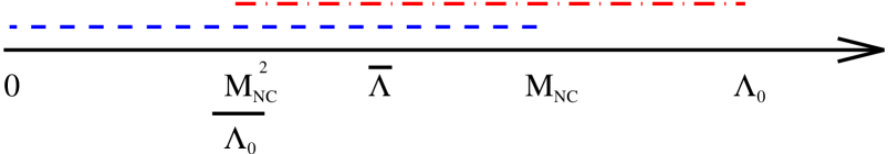
Figure 4: The two overlapping ranges in which a Wilsonian picture holds

5.1 Matching two Wilsonian flows

From the above analysis we learn that the Wilsonian picture does not hold straightforwardly from a very high scale $\Lambda=\Lambda_{0}\gg M_{NC}$ down to $\Lambda=0$. Nevertheless, it may be partially recovered as a two-steps procedure, in which the high-energy theory is matched to a low-energy one at a intermediate scale $\bar{\Lambda}$ such that $M_{NC}^{2}/\Lambda_{0}\ll\bar{\Lambda}\ll M_{NC}$. $\bar{\Lambda}$ lies in the region in which the Wilsonian picture holds for both the high-energy and the low-energy RG flows. Then, once the $\Lambda_{0}$-dependence is absorbed in the relevant couplings of the high-energy theory, it does not enter the matching conditions to the low-energy one at $\bar{\Lambda}$ . Since the RG flow for $\Lambda,\,p\mathrel{\vbox{\hbox{$<$}\nointerlineskip\hbox{$\sim$}}}\bar{\Lambda}$ is that of a commutative theory, the low-energy theory knows about non-commutativity only via its boundary conditions, i.e. the matching conditions at $\bar{\Lambda}$. In the following we illustrate this procedure explicitly at one-loop.

By giving boundary conditions at $\Lambda_{0}$, the relevant couplings of the high-energy theory are

$$\gamma_{3}^{h}(\Lambda)=\gamma_{3}^{h}(\Lambda_{0})+\frac{g^{2}}{32\pi^{2}}\left[\frac{2}{3}\Lambda_{0}^{2}-\frac{4}{3\tilde{p}_{0}^{2}}J_{0}(\Lambda_{0}\tilde{p_{0}})-(\Lambda_{0}\to\Lambda)\right]$$

$$\gamma_{2}^{h}(\Lambda)=\gamma_{2}^{h}(\Lambda_{0})+\frac{g^{2}}{24\pi^{2}}\frac{1}{p_{0}^{2}\tilde{p_{0}}^{2}}\left[J_{0}(\Lambda_{0}\tilde{p_{0}})+\frac{\Lambda_{0}\tilde{p_{0}}}{2}J_{1}(\Lambda_{0}\tilde{p_{0}})-(\Lambda_{0}\to\Lambda)\right]\;\;\;\;$$

$$\gamma_{4}^{h}(\Lambda)=\gamma_{4}^{h}(\Lambda_{0})+\frac{g^{4}}{48\pi^{2}}\log\frac{\Lambda^{2}}{\Lambda_{0}^{2}}+\cdots\;\;\;\;\;\;\;\;(m^{2}\ll p_{0}^{2},\;\Lambda^{2})\,,$$ (55)

where dots are exponentially suppressed terms, while for the low-energy theory they are given by the same expressions with the substitutions

$$``h^{\prime\prime}\to``l^{\prime\prime},\;\;\;\;\;\;\;\;\;\Lambda_{0}\to\bar{\Lambda}.$$ (56)

The $\Lambda_{0}$ dependence in (5.1) can be absorbed in the boundary conditions $\gamma_{2,3,4}^{h}(\bar{\Lambda})$, and the matching conditions for the relevant couplings are trivially given by

$$\gamma_{2,3,4}^{h}(\bar{\Lambda})=\gamma_{2,3,4}^{l}(\bar{\Lambda}).$$ (57)

Besides the relevant couplings, we have also to impose matching conditions on the two irrelevant ones $\Delta^{2}_{\Lambda,\Lambda_{0}}$ and $\Delta^{4}_{\Lambda,\Lambda_{0}}$. We start by discussing $\Delta^{2}_{\Lambda,\Lambda_{0}}$. For the high-energy theory, $\Delta^{2,h}_{\Lambda,\Lambda_{0}}(p)$ is given by eq. (4), while for the low-energy one, $\Delta^{2,l}_{\Lambda,\bar{\Lambda}}(p)$, we have to perform the same substitution as in eq. (56) and to add the initial condition $\Delta^{2,l}_{\bar{\Lambda},\bar{\Lambda}}(p)$(the initial conditions at $\Lambda_{0}$ for the irrelevant couplings of the high energy theory are taken to be zero, as in eq. (4)).

To fix the matching conditions we first take $\Lambda=\bar{\Lambda}$ and set the external momenta at some $P=O(\bar{\Lambda})$. Equating the irrelevant couplings for the two theories we get,

$$\Delta^{2,l}_{\bar{\Lambda},\bar{\Lambda}}(P) =\Delta^{2,h}_{\bar{\Lambda},\Lambda_{0}}(P)$$ (58)

$$=\frac{g^{2}}{24\pi^{2}}\left\{\frac{J_{0}(\bar{\Lambda}\tilde{P})}{\tilde{P}^{2}}-\frac{J_{0}(\bar{\Lambda}\tilde{p_{0}})}{\tilde{p_{0}}^{2}}+\frac{{P}^{2}-p_{0}^{2}}{p_{0}^{2}\tilde{p_{0}}^{2}}\left[J_{0}(\bar{\Lambda}\tilde{p_{0}})+\frac{\bar{\Lambda}\tilde{p_{0}}}{2}J_{1}(\bar{\Lambda}\tilde{p_{0}})\right]\right\}$$

$$\;\;\;\;\;+({\mathrm{exp.\;suppressed\;terms\;in\;}}\Lambda_{0}),$$

where we have neglected the terms in $\Lambda_{0}$ since, due to or choice for the external momenta $P$ (and for $p_{0}$, which we take in the same range), they are exponentially suppressed. Now, we choose the boundary conditions for momenta $p\leq O(P)$ by using the same expression (58), i.e we neglect the $\Lambda_{0}$-terms for any value of the external momenta,

$$\Delta^{2,l}_{\Lambda,\bar{\Lambda}}(p)=\Delta^{2,l}_{\bar{\Lambda},\bar{\Lambda}}(p)$$

$$+\frac{g^{2}}{24\pi^{2}}\left\{\frac{J_{0}(\Lambda\tilde{{p}})}{\tilde{{p}}^{2}}-\frac{J_{0}(\Lambda\tilde{p_{0}})}{\tilde{p_{0}}^{2}}+\frac{{p}^{2}-p_{0}^{2}}{p_{0}^{2}\tilde{p_{0}}^{2}}\left[J_{0}(\Lambda\tilde{p_{0}})+\frac{\Lambda\tilde{p_{0}}}{2}J_{1}(\Lambda\tilde{p_{0}})\right]-(\Lambda\to\bar{\Lambda)}\right\}$$

$$\;\;\;\;=\frac{g^{2}}{24\pi^{2}}\left[\frac{1}{\tilde{p}^{2}}-\frac{1}{\tilde{p_{0}}^{2}}+\frac{p^{2}-p_{0}^{2}}{p_{0}^{2}\tilde{p}_{0}^{2}}\right]+O({\Lambda}^{4}\tilde{p}^{2},\,\Lambda^{4}\tilde{p}_{0}^{2}),$$ (59)

where $\Delta^{2,l}_{\bar{\Lambda},\bar{\Lambda}}(p)$ is given by eq. (58)) for $P\to p$. Notice that the contribution to $\Delta^{2,l}_{\Lambda,\bar{\Lambda}}(p)$ comes mainly from its boundary condition at $\bar{\Lambda}$. The running from $\bar{\Lambda}$ downwards contributes with $O(\bar{\Lambda}^{4}p^{4}/M_{NC}^{8})$ suppressed terms, consistent with the fact that $\Delta^{2}_{\Lambda,\bar{\Lambda}}(p)$ is zero at one-loop in the commutative theory.

Analogously for the four-point irrelevant vertex we impose

$$\Delta^{4,l}_{\bar{\Lambda},\bar{\Lambda}}(P_{i})=\Delta^{4,h}_{\bar{\Lambda},\Lambda_{0}}(P_{i})\,,$$ (60)

and, neglecting the $\Lambda_{0}$ terms for lower external momenta, we get (in the $\Lambda\to 0$ limit)

$$\lim_{\Lambda\to 0}\Delta^{4,l}_{\bar{\Lambda},\bar{\Lambda}}(p_{i})\simeq \frac{g^{4}}{32\pi^{2}}\log\left(\frac{(p_{1}+p_{2})^{2}}{p_{0}^{2}}\right)-\frac{g^{4}}{144\pi^{2}}\left[\log\left(\frac{p_{0}^{2}(\tilde{\bar{p}}_{1}+\tilde{\bar{p}}_{2})^{2}}{4}\right)+\frac{1}{2}\sum_{i}\log\frac{(p_{0}^{2}\tilde{\bar{p}}_{i}^{2})}{4}\right.$$ (61)

$$\left.+\frac{1}{4}\log\left(\frac{p_{0}^{2}(\tilde{\bar{p}}_{1}+\tilde{\bar{p}}_{4})^{2}}{4}\right)+\frac{1}{4}\log\left(\frac{p_{0}^{2}(\tilde{\bar{p}}_{1}+\tilde{\bar{p}}_{3})^{2}}{4}\right)\right]$$

$$+(2\to 3)+(2\to 4).$$

The first logarithm above is just the 1-loop four-point function of the commutative theory, the rest is the contribution coming from the boundary condition at $\bar{\Lambda}$.

From the low-energy point of view, the information that the original high energy theory is non-commutative is encoded in the boundary conditions at $\bar{\Lambda}$ for the three relevant couplings plus those for the two irrelevant ones $\Delta^{2}_{\Lambda,\bar{\Lambda}}$ $\Delta^{4}_{\Lambda,\bar{\Lambda}}$. This is to be contrasted with the usual Wilsonian picture, where the dependence on the boundary conditions of all the irrelevant couplings vanishes at low energies as some powers of $p/\bar{\Lambda}$. Indeed, this is exactly what makes a theory predictive, in that it depends only on a finite number of boundary conditions. In the non-commutative case, the new scale $M_{NC}$ gives rise to terms like $1/\tilde{p}^{2}$ and $\log{\tilde{p}}$ which do not decouple when $M_{NC}\gg\bar{\Lambda}\gg p\to 0$. Fortunately such terms enter only $\Delta^{2}_{\Lambda,\bar{\Lambda}}$ and $\Delta^{4}_{\Lambda,\bar{\Lambda}}$, but not $\Gamma_{2n}$ for $n\geq 3$, as can be checked dimensionally. Thus, the boundary conditions for the latter couplings become more and more irrelevant as $p,\Lambda\to 0$ and the low-energy theory is still predictive –and $\Lambda_{0}$-independent– although it needs two extra boundary conditions compared to the commutative case.

From the point of view of the low-energy observer, the two extra boundary conditions might come from some high-energy degrees of freedom, as discussed in [7]. Also in that picture, once the extra degrees of freedom are integrated out, a commutative theory with the bizarre propagator $(p^{2}+g^{2}/24\pi^{2}\tilde{p}^{2})^{-1}$ is obtained. However, in the case of the massive theory, the reproduction of the logarithmic $\tilde{p}$ behavior by the same means turns out to be not so straightforward.

6 Summary and outlook

The Wilsonian RG equations (3.2) exhibit a remarkable momentum ordering; a given irrelevant coupling evaluated at cut-off $\Lambda$ receives contributions only from loop momenta $\lambda\geq\Lambda$. In this paper we have used this basic property in order to split the analysis of the perturbative behavior of the non-commutative scalar theory in two steps. First, by taking $\Lambda$ much larger than any physical mass scale, we have inspected the UV sector of the theory. In this regime, if the external momenta are all $\gg M_{NC}^{2}/\Lambda_{0}$, the contribution of the non-planar diagrams is damped by the non-commutative phases while that of the planar ones is the same as for the commutative theory. The proof of perturbative renormalizability at any order in perturbation theory is then just a straightforward generalization of that given for the commutative case in [16, 17].

Then we turned to the IR sector by lowering $\Lambda$ towards the physical limit, $\Lambda\to 0$. In this regime the well-known IR/UV connection spoils perturbation theory completely, as IR divergences appear in the contributions to any Green function. The IR divergences can be completely resummed in a way analogous to what is customarily done in finite temperature field theory, i.e. by using a resummed propagator and introducing a corresponding counterterm in the interaction lagrangian. The resummation procedure does not change the UV sector of the theory, so that the previous discussion of UV renormalizability holds unaltered. In the resummed theory we were able to compute the next-to-leading corrections to the two-point functions, which exhibit a non-analytic dependence on the coupling constant.

Finally, we discussed what survives in the non-commutative case of the usual Wilsonian picture, i.e. insensitivity of the theory at long distance to the short distance behavior after proper redefinition of the relevant couplings. At first sight, the IR/UV connection seems to spoil completely this picture. Indeed, since in the resummed theory the IR/UV connection affects only the two- and four- point functions, the situation is less dramatic. The high-energy theory can be matched to a low-energy one which in the IR limit has a purely commutative RG flow and knows about non-commutativity only via the boundary conditions of the two- and four- point functions. If the scale at which the high-energy theory is defined, $\Lambda_{0}$, is well above the non-commutative scale, the low-energy theory sensitivity to $\Lambda_{0}$ is exponentially suppressed.

The present study opens a series of questions. The first one is the extension of this analysis to gauge theories. The main problem in that context is gauge invariance, which is broken by the introduction of a momentum cut-off and can be recovered only in the physical limit $\Lambda\to 0$, $\Lambda_{0}\to\infty$. At finite values of the cut-off the theory satisfies modified Ward identities which were discussed for the commutative case in [23]. In that paper it was shown how gauge invariance can be controlled order by order in perturbation theory in such a way as to be recovered in the physical limit. The extension of those results to the non-commutative case requires close scrutiny, the main complication being the need of a resummation in order to get a finite $\Lambda\to 0$ limit. It is not presently clear to us how such a resummation can be performed. It is evident that the simple resummation of the self-energy in the propagator is not a gauge invariant operation. Again, the example of thermal field theories might be of help for us. In the pure QCD case, Ward identities connect n to n+1-point functions, so that not only the gluon self-energy has to be resummed, but all n-gluon functions. The program was achieved by Braaten and Pisarski and leads to to the well known Hard Thermal Loop effective action [18]. It would be very interesting to understand if an analogous result can be obtained in the non-commutative case.

Another interesting issue is that of phase transition and the critical regime. Indeed some analysis at one-loop have been already presented in ref.  [24], but we argue that the actual behavior should be quite different from that discussed in that paper. The point is that, being higher loops IR divergent, the study of the critical regime can be consistently performed only in the resummed theory, which has the propagator $(p^{2}+m^{2}+g^{2}/24\pi^{2}\tilde{p}^{2})^{-1}$. So, the long distance $p\to 0$ limit is dominated by the $g^{2}/24\pi^{2}\tilde{p}^{2}$ term and turns out to be insensitive to the sign of $m^{2}$, which usually determines whether the vacuum breaks or not the symmetry. Thus we conclude that there are no phase transitions in these theories, at least of the common type. In the RG language, the flow shuts-off well before the mass can be probed ( if $g^{2}M_{NC}^{4}/m^{4}\gg 1$) and the critical exponents are drastically changed with respect to those of the massless commutative theory. This agrees with the evidences for a non-homogeneous phase discussed in ref. [25].

Appendix A Appendix

We have at one-loop that

$$\gamma_{4}(\Lambda)=I_{4}^{(p)}+I_{4}^{(np)},$$ (62)

where the integrals defining $\gamma_{4}(\Lambda)$ are

$$I_{4}^{(p)} =\frac{2g^{4}}{3}\int\frac{d^{4}q}{(2\pi)^{4}}\frac{\Theta(\Lambda^{2}-q^{2})\Theta(\bar{p}^{2}-2\bar{p}q)}{(q^{2}+m^{2})[(q-\bar{p})^{2}+m^{2}]}$$

$$I_{4}^{(np)} =\frac{g^{4}}{9}\frac{1}{h(\bar{p}_{1},\bar{p}_{2},\bar{p}_{3},\bar{p}_{4})}\int\frac{d^{4}q}{(2\pi)^{4}}\frac{\Theta(\Lambda^{2}-q^{2})\Theta(\bar{p}^{2}-2\bar{p}q)}{(q^{2}+m^{2})[(q-\bar{p})^{2}+m^{2}]}F(q,\bar{p}_{i})$$ (63)

$$+(\bar{p}_{2}\to\bar{p}_{3})+(\bar{p}_{2}\to\bar{p}_{4}).$$

$F(q,\bar{p}_{i})$ is defined as

$$F(q,\bar{p}_{i}) =2\cos\bar{p}_{12}\cos\bar{p}_{34}\cos(\bar{p}\cdot\tilde{q})+\cos\bar{p}_{34}\left[\cos\left(\bar{p}_{12}+\bar{p}_{1}\cdot\tilde{q}\right)+\cos\left(\bar{p}_{21}+\bar{p}_{2}\cdot\tilde{q}\right)\right]$$ (64)

$$+\cos\bar{p}_{21}\left[\cos\left(\bar{p}_{43}+\bar{p}_{4}\cdot\tilde{q}\right)+\cos\left(\bar{p}_{34}+\bar{p}_{3}\cdot\tilde{q}\right)\right]$$

$$+\frac{1}{2}\cos\left[\bar{p}_{12}+\bar{p}_{34}+\left(\bar{p}_{1}+\bar{p}_{4}-\bar{p}_{2}-\bar{p}_{3}\right)\cdot\tilde{q}\right]$$

$$+\frac{1}{2}\cos\left[p_{12}-p_{34}+\left(\bar{p}_{1}-\bar{p}_{4}-\bar{p}_{2}+\bar{p}_{3}\right)\cdot\tilde{q}\right].$$

The planar contribution $I_{4}^{(p)}$ is evaluated for $\Lambda\gg p_{0}\gg m$

$$\frac{g^{2}}{12\pi^{3}}\int_{\frac{p_{0}}{2}}^{\Lambda}dq^{2}\int^{1}_{0}dx\sqrt{1-x^{2}}\frac{1}{q^{2}+p_{0}^{2}+2\bar{p}qx}\simeq\frac{1}{48\pi^{2}}\log\frac{\Lambda^{2}}{p_{0}^{2}}.$$ (65)

The generic integral involved in the non-planar part is

$$\int\frac{d^{4}q}{(2\pi)^{4}}\frac{\Theta(\Lambda^{2}-q^{2})\Theta(\bar{p}^{2}-2\bar{p}q)}{(q^{2}+m^{2})((q-\bar{p})^{2}+m^{2})}\cos(a+b\cdot\tilde{q}).$$ (66)

Assuming $\Lambda$ very large

$$\simeq\frac{1}{4\pi^{3}} \left[\cos a\int_{0}^{1}dx\sqrt{1-x^{2}}\left({\rm ci}(\Lambda\tilde{b}x)-{\rm ci}(\frac{p_{0}\tilde{b}x}{2})\right)+\right.$$ (67)

$$\left.\sin a\int_{0}^{1}dx\sqrt{1-x^{2}}\left({\rm si}(\Lambda\tilde{b}x)-{\rm si}(\frac{p_{0}\tilde{b}x}{2})\right)\right],$$

where we have introduced the sine-integral and the cosine-integral functions. As $\Lambda\to\infty$ both ${\rm ci}(\Lambda\tilde{b}x)$ and ${\rm si}(\Lambda\tilde{b}x)$ goes to zero. Taking instead $\Lambda$ finite and $\tilde{b}\to 0$, and using

$${\rm ci}(\Lambda\tilde{b}x)-{\rm ci}(\frac{p_{0}\tilde{b}x}{2})\simeq\log\frac{2\Lambda}{p_{0}}+O(\tilde{b}),$$

$${\rm si}(\Lambda\tilde{b}x)-{\rm si}(\frac{p_{0}\tilde{b}x}{2})\simeq O(\tilde{b}),$$ (68)

we obtain that the leading contribution is commutative-like

$$\simeq\cos a\log\frac{\Lambda^{2}}{p_{0}^{2}}$$

, while as $\Lambda\to\infty$ the dominant term is

$$-\frac{1}{4\pi^{3}}\cos a\int_{0}^{1}dx\sqrt{1-x^{2}}{\rm ci}(\frac{p_{0}\tilde{b}x}{2}).$$ (69)

For $p_{0}\tilde{b}\gg 1$ the contribution is very small while as $p_{0}\tilde{b}\leq 1$ we can expand the integral using eq. (68) and to recover eq. (38) where the explicit form of $F(q,\bar{p}_{i})$ has been used.

Concerning $\Delta^{4}_{\Lambda\Lambda_{0}}$ we have a similar separation (at one-loop):

$$\Delta^{4}_{\Lambda\Lambda_{0}}=\Delta^{4}_{p}+\Delta^{4}_{np},$$ (70)

where for $\Lambda_{0}\to\infty$ we have

$$\Delta^{4}_{(p)} =\frac{2g^{4}}{9}\int\frac{d^{4}q}{(2\pi)^{4}}\left[\frac{\cos p_{12}\cos p_{34}}{h(p_{i})}\frac{\Theta(q^{2}-\Lambda)\Theta({p}^{2}-2{p}q)}{(q^{2}+m^{2})((q-p)^{2}+m^{2})}-(p\to\bar{p})\right]_{p=p_{1}+p_{2}}$$ (71)

$$+(p_{2}\to p_{3})+(p_{2}\to p_{4})$$

$$=\frac{g^{4}}{18\pi^{3}}\int dq~{}q\int_{0}^{1}dx\sqrt{1-x^{2}}\left[\frac{\cos p_{12}\cos p_{34}}{h(p_{i})(q^{2}+p^{2}-2pqx)}-(p\to\bar{p})\right]_{p=p_{1}+p_{2}}$$

$$+(p_{2}\to p_{3})+(p_{2}\to p_{4}).$$

For large $\Lambda$ we can expand the denominators retaining the linear terms and obtaining therefore the first term in eq. (39). The non-planar part is instead suppressed in the same limit: the typical contributions have the form

$$\int_{\Lambda}^{+\infty}\frac{dq}{q}\int_{-1}^{1}dx\sqrt{1-x^{2}}\cos(\tilde{b}qx)\simeq\int_{\Lambda}^{+\infty}\frac{dq}{q}\frac{J_{1}(\tilde{b}q)}{\tilde{b}q}.$$ (72)