April 2001 UMTG–228
hep-th/0104199

Beyond the Elliptic Genus
Orlando Alvarez
Department of Physics
University of Miami
P.O. Box 248046
Coral Gables, FL 33146 USA
and

I. M. Singer
Department of Mathematics
Massachusetts Institute of Technology
77 Massachusetts Avenue, Rm. 2–387
Cambridge, MA 02139 USA

Given a Riemann surface $\Sigma$ and a riemannian manifold $M$ with certain restrictions, we construct a cobordism invariant of $M$. This invariant is a generalization of the elliptic genus and it shares some similar properties.

1 Introduction

The analytic index of an elliptic differential operator $D:C^{\infty}(E_{+})\to C^{\infty}(E_{-})$ between vector bundles over a manifold $M$ is defined as

$$\operatorname{Index}(D)=\dim\ker D-\dim\operatorname{coker}D^{*}\;.$$ (1.1)

This index can be computed by using heat evolution operators. There are two natural laplacians associated with the elliptic operator $D$:

$$\Delta_{+} = D^{*}D:C^{\infty}(E_{+})\to C^{\infty}(E_{+})\;,$$ (1.2)

$$\Delta_{-} = DD^{*}:C^{\infty}(E_{-})\to C^{\infty}(E_{-})\;.$$ (1.3)

The index may be expressed as

$$\operatorname{Index}(D)=\operatorname*{Tr}\exp(-t\Delta_{+})-\operatorname*{Tr}\exp(-t\Delta_{-})\;,t>0,$$ (1.4)

because if $\Delta_{+}\phi=\lambda\phi$, then $\Delta_{-}(D\phi)=\lambda(D\phi)$. Thus all but the $1$ eigenvalues of $e^{-t\Delta_{+}}$ cancel those of $e^{-t\Delta_{-}}$ in the difference of the traces. The cancellation is incomplete because one cannot identify $\ker D$ with $\ker D^{*}$. Using heat operators leads one to attempt to find a classical quantum mechanics problem with the laplacians being the hamiltonians. The end result is supersymmetric quantum mechanics which has a supersymmetric path integral formulation [1, 2, 3].

We can go beyond quantum mechanics to quantum field theory and ask whether there are generalizations of the index theorem. In the context of $(1+1)$ dimensional quantum field theories, the answer is yes in the form of the elliptic genus [4, 5, 6, 7, 8]. For a survey of the mathematical literature look in [9]. The $(1+1)$ dimensional field theory is formulated on a torus where there is a notion of a hamiltonian, i.e., laplacian. Formally, the elliptic genus is the $S^{1}$-index of a formal differential operator, the Dirac-Ramond operator, the Dirac operator with potential function Clifford multiplication by $x^{\prime}(\sigma)$ on the loop space $LM$. If one goes beyond genus one the Hamiltonian interpretation is lost, but there is still a path integral. Can one make any sense of this path integral as some generalization of the index and what is it? In this paper we show that the semiclassical approximation of the path integral gives a cobordism invariant generalizing the elliptic genus to the case of genus $g>1$.

In Section 2 we review the supersymmetric sigma model, its action and partition function. We explain in Section 3 conditions needed on the target manifold to cancel anomalies and make the path integral formally well defined. We derive the semiclassical approximation in Section 4, obtaining the semiclassical partition function as a ratio of determinants in (4.12). The semiclassical limit is “topological” but not a topological quantum field theory [10, 11].

We derive a differential equation for one of these determinants in Section 5 and use it to ultimately compute the determinant in terms of $\vartheta$-functions whose characteristics are determined in Appendix A. We identify the $\vartheta$-function with a cross section of our determinant line bundle in Section 6. Using an explicit construction of the determinant line bundle (Section 7) we compute $\det_{\mathbf{1}^{\perp}}\raisebox{-1.07639pt}{\large$\Box$}_{-}$ in Section 8 (Theorem 8.14). In Section 9 we discuss our final formula which gives a cobordism invariant generalizing the elliptic genus as we explain. There we obtain a simple “relative invariant” by taking ratios.

In the appendices we tried to make explicit known material in algebraic geometry.

The body of the paper was written over two years ago. We had hoped to exhibit our semiclassical partition function explicitly as a nonholomorphic section of a holomorphic line bundle over spin moduli space. We did not succeed in doing so. In the meantime line bundles over jacobians have received considerable attention because of M-theory (partition functions for self-dual fields and chiral anomalies). Though we are aware of some of these developments [12, 13], we have not incorporated their viewpoint into our computations.

2 The Supersymmetric Sigma Model

2.1 The bosonic model

Let $\Sigma$ be a Riemann surface of genus $g$ and let $M$ be a connected and oriented riemannian manifold of dimension $d$. Consider a map $X:\Sigma\to M$; then the classical nonlinear sigma model is defined by the “energy” action

$$I(X)=\frac{1}{2}\left\langle dX,dX\right\rangle\;,$$ (2.1)

where $dX$ denotes the differential map $dX:T\Sigma\to TM$. The natural inner product induced by the riemannian structures is denoted by angular brackets. If $(x^{1},x^{2})$ are real local coordinates on $\Sigma$ and if we abuse notation and also denote local coordinates on $M$ by $X$, action (2.1) may be written in the form

$$I(X) = \frac{1}{2}\int_{\Sigma}d^{2}x\;\sqrt{\det\gamma}\;\gamma^{ab}(x)\,g_{\mu\nu}(X(x)){\partial X^{\mu}\over\partial x^{a}}{\partial X^{\nu}\over\partial x^{b}}$$ (2.2)

$$= i\int_{\Sigma}g_{\mu\nu}(X(x))\partial X(x)^{\mu}\wedge\bar{\partial}X(x)^{\nu}\;.$$ (2.3)

In the first line, $\gamma_{ab}(x)dx^{a}\otimes dx^{b}$ is the riemannian metric on $\Sigma$, and $g_{\mu\nu}(X)dX^{\mu}\otimes dX^{\nu}$ is the riemannian metric on $M$. In the second line we have exploited the complex structure on $\Sigma$ induced by its riemannian structure to write the action in a way that depends manifestly only on the complex structure.

2.2 The supersymmetric model

The chiral Dirac operator on a Riemann surface $\bar{\partial}_{1/2}:\Lambda^{1/2,0}(\Sigma)\to\Lambda^{1/2,1}(\Sigma)$ has numerical index zero. It is also a skew symmetric operator and consequently has a $\operatorname{mod}2$ index, $(\dim\ker\bar{\partial}_{1/2})\operatorname{mod}2$ which is a topological invariant. An even spin structure is one where $\dim\ker\bar{\partial}_{1/2}=0\operatorname{mod}2$ and an odd spin structure is one where $\dim\ker\bar{\partial}_{1/2}=1\operatorname{mod}2$, see [14].

The supersymmetric version of action (2.1) requires the introduction of a fermionic field $\psi$ which is a section of the bundle $K^{1/2}\otimes X^{*}(TM)$ where $K$ is the canonical bundle on $\Sigma$. We have to pick a square root of the canonical bundle, i.e., a spin structure $s$ on $\Sigma$. Later we will see that we have to pick an odd spin structure. Let $\stackrel{{\scriptstyle\circ}}{{\nabla}}\kern-2.15277pt\vphantom{\nabla}_{X}$ be the induced Riemannian covariant differential on the bundle $K^{1/2}\otimes X^{*}(TM)$. If we use the complex structure on $\Sigma$ and decompose the tangent bundle as $T\Sigma=T^{1,0}\Sigma\oplus T^{0,1}\Sigma$ then the differential has a natural decomposition as $\stackrel{{\scriptstyle\circ}}{{\nabla}}\kern-2.15277pt\vphantom{\nabla}_{X}=\stackrel{{\scriptstyle\circ}}{{\nabla}}\kern-2.15277pt\vphantom{\nabla}_{X}^{1,0}+\stackrel{{\scriptstyle\circ}}{{\nabla}}\kern-2.15277pt\vphantom{\nabla}_{X}^{0,1}$. In local coordinates, the covariant derivative of the section

$$\psi^{\mu}\;\sqrt{dz}\otimes{\partial\over\partial X^{\mu}}\;,$$ (2.4)

is given by

$$\left(\stackrel{{\scriptstyle\circ}}{{\nabla}}\kern-2.15277pt\vphantom{\nabla}_{X}^{0,1}\psi\right)^{\mu}=\bar{\partial}\psi^{\mu}+(\bar{\partial}X^{\lambda})\,\stackrel{{\scriptstyle\circ}}{{\Gamma}}\kern-2.15277pt\vphantom{\Gamma}^{\mu}_{\lambda\nu}(X)\psi^{\nu}\;,$$ (2.5)

where $\stackrel{{\scriptstyle\circ}}{{\Gamma}}\kern-2.15277pt\vphantom{\Gamma}^{\mu}_{\lambda\nu}$ are the Christoffel symbols for the Riemannian connection on $TM$.

The supersymmetry transformation laws are

$$\delta X = \epsilon\psi$$ (2.6)

$$\delta\psi = \epsilon\partial_{z}X\;,$$ (2.7)

where $\epsilon$ is a local holomorphic section of $K^{-1/2}$. For the mathematicians, $\delta X$ should be interpreted as a tangent vector to the space of maps $\operatorname{Map}(\Sigma,M)$, i.e., a cross section of $X^{*}(TM)$. The naive supersymmetric action may be written in local complex coordinates as

$$I=I_{g}+I_{B}\;,$$ (2.8)

where

$$I_{g} = i\int_{\Sigma}dz\wedge d\bar{z}\;g_{\mu\nu}(X(z))\partial_{z}X^{\mu}\partial_{\bar{z}}X^{\nu}$$ (2.9)

$$+ i\int_{\Sigma}dz\wedge d\bar{z}\;g_{\mu\nu}(X)\left(\partial_{\bar{z}}\psi^{\mu}+(\partial_{\bar{z}}X^{\lambda})\stackrel{{\scriptstyle\circ}}{{\Gamma}}\kern-2.15277pt\vphantom{\Gamma}^{\mu}_{\lambda\rho}(X)\psi^{\rho}\right)\psi^{\nu}\;,$$

$$= i\int_{\Sigma}g_{\mu\nu}(X)\left(\partial X^{\mu}\wedge\bar{\partial}X^{\nu}+(\stackrel{{\scriptstyle\circ}}{{\nabla}}\vphantom{\nabla}_{X}^{0,1}\psi)^{\mu}\psi^{\nu}\right)\;;$$ (2.10)

and

$$I_{B}=i\int_{\Sigma}dz\wedge d\bar{z}\left(B_{\mu\nu}(X)\partial_{z}X^{\mu}\partial_{\bar{z}}X^{\nu}+\frac{1}{2}C_{\lambda\mu\nu}(X)\psi^{\lambda}\psi^{\mu}\partial_{\bar{z}}X^{\nu}\right)\;.$$ (2.11)

For the moment, we take $B=\frac{1}{2}B_{\mu\nu}dX^{\mu}\wedge dX^{\nu}$ to be a real $2$-form on $M$ with

$$C=dB=\frac{1}{3!}\;C_{\mu\nu\rho}\;dX^{\mu}\wedge dX^{\nu}\wedge dX^{\rho}\;.$$ (2.12)

We will be more precise later on the exact interpretation of the $B$ term. For now suffices to say that it is required for anomaly cancellation.

The action is not invariant under supersymmetry in genus larger than one. For example, the transformation law for action $I_{g}$ under the supersymmetry transformation is

$$\delta I_{g}=\int_{\Sigma}\epsilon\partial_{z}\left(g_{\mu\nu}(X)\psi^{\mu}\partial_{\bar{z}}X^{\nu}\right)\;.$$ (2.13)

For the supersymmetry to be a symmetry of this action, $\epsilon$ must be holomorphic and this only happens in genus zero or genus one. Note that in genus one, a constant $\epsilon$ tells us that $\psi$ must belong to an odd spin structure, a consequence of the SUSY transformation laws and the periodicity of $X$ around any cycle in $\Sigma$. Therefore the field $\psi$ is periodic on a torus, the boundary condition that is consistent with supersymmetry. For genus $g>1$, there is no global supersymmetry and one can only talk about supersymmetry locally. The classical holomorphic supercurrent is of type $(3/2,0)$.

The above action defines a sensible classical conformal field theory. Quantum mechanically, this is not so. Firstly, there are global fermionic anomalies as discussed in [16, 17] and local Adler-Bell-Jackiw anomalies associated with gauge transformations in $TM$. The $I_{B}$ term is used to eliminate these anomalies. Secondly, due to the conformal anomaly, the above is not in general a conformal field theory. But we will only use the semiclassical approximation about a constant background, which is a conformal field theory.

3 The Supersymmetric Path Integral

3.1 Full theory

The path integral for action (2.8) involves integrating over all maps from $\Sigma$ to $M$ and integrating over all fermionic sections of $K^{1/2}\otimes X^{*}(TM)$. Since the fermions enter quadratically, we can perform the fermionic integral obtaining the following formal expression for the partition section

$$Z(g_{\mu\nu},\gamma_{ab},s) = \int\limits_{\operatorname{Map}(\Sigma,M)}[{\cal D}X]\;\operatorname{pf}(\nabla_{X}^{0,1})\;$$ (3.1)

$$\times \exp\left\{i\int_{\Sigma}dz\wedge d\bar{z}\;\left[g_{\mu\nu}(X(z))+B_{\mu\nu}(X(z))\right]\partial_{z}X^{\mu}\partial_{\bar{z}}X^{\nu}\right\}\;.$$

In the above, $\nabla_{X}^{0,1}$ is defined just like (2.5) except that the connection coefficients are given by

$$\Gamma^{\lambda}_{\mu\nu}=\stackrel{{\scriptstyle\circ}}{{\Gamma}}\kern-2.15277pt\vphantom{\Gamma}^{\lambda}_{\mu\nu}+\frac{1}{2}C_{\mu}{}^{\lambda}{}_{\nu}\;.$$ (3.2)

This is a metric compatible connection with torsion. In the expression for the partition section (3.1), $\operatorname{pf}(\nabla_{X}^{0,1})$ is the pfaffian section of the pfaffian line bundle $\operatorname{PF}(\nabla_{X}^{0,1})$. We emphasize that the partition section depends on the metric on the target space $M$, the metric on the Riemann surface $\Sigma$, and the spin structure $s$ of the Riemann surface.

The expression for the partition section $Z$ may be interpreted as an averaging of the pfaffian section over $\operatorname{Map}(\Sigma,M)$. This can be done only if the pfaffian line bundle is a trivial line bundle over $\operatorname{Map}(\Sigma,M)$. If not we have an anomaly in the sigma model as discussed in [16, 17]. General arguments tell us that the determinant line bundle $\operatorname{DET}(\nabla_{X}^{0,1})\to\operatorname{Map}(\Sigma,M)$ exists over compact sets of $\operatorname{Map}(\Sigma,M)$. On such sets it has a canonical section $\det(\nabla_{X}^{0,1})$ because $\operatorname{Index}\nabla_{X}^{0,1}=0$. Freed’s Theorem 3.1 [18] guarantees that there exists a line bundle $\operatorname{PF}(\nabla_{X}^{0,1})$ with a canonical isomorphism $\operatorname{PF}(\nabla_{X}^{0,1})\otimes\operatorname{PF}(\nabla_{X}^{0,1})=\operatorname{DET}(\nabla_{X}^{0,1})$ and with a canonical section $\operatorname{pf}\nabla_{X}^{0,1}$ such that $(\operatorname{pf}\nabla_{X}^{0,1})^{\otimes 2}=\det(\nabla_{X}^{0,1})$. Since the pfaffian line bundle $\operatorname{PF}(\nabla_{X}^{0,1})\to\operatorname{Map}(\Sigma,M)$ must be trivial to prevent the anomaly, the line bundle $\operatorname{DET}(\nabla_{X}^{0,1})\to\operatorname{Map}(\Sigma,M)$ must also be trivial. The family’s index theorem shows that the first Chern class of the determinant line bundle is given by

$$\operatorname{c}_{1}(\operatorname{DET}(\nabla_{X}^{0,1}))=-\frac{1}{2}\int_{\Sigma}\operatorname{ev}^{*}[\operatorname{p}_{1}(M)]\;,$$ (3.3)

where $\operatorname{ev}:\Sigma\times\operatorname{Map}(\Sigma,M)\to M$ is the evaluation map. The cohomology class $2\pi\operatorname{c}_{1}(\operatorname{DET}(\nabla_{X}^{0,1}))$ may be represented by a curvature $2$-form $\mathcal{F}$ of the determinant line bundle $\operatorname{DET}(\nabla_{X}^{0,1})$ (which comes equipped with a Quillen connection). $\mathcal{F}/2\pi=-\frac{1}{2}\int_{\Sigma}\operatorname{ev}^{*}\operatorname{p}_{1}(M)=-\frac{1}{2}\int_{X(\Sigma)}\operatorname{p}_{1}(M)$ at $X\in\operatorname{Map}(\Sigma,M)$, see Bismut and Freed [19, 20]. We assume that $\dim M$ is even and greater than $2$. We also assume that $\pi_{j}(M)=0$ for $j\leq 3$. The condition $\pi_{3}(M)=0$ greatly simplifies the analysis. We discuss complications when $\pi_{3}(M)\neq 0$ later. Our assumptions on $M$ imply that $M$ is an oriented, connected spin manifold and that $\pi_{j}(\operatorname{Map}(\Sigma,M))=0$ for $j=0,1$. Hence $\operatorname{PF}(\nabla_{X}^{0,1})$ is the unique square root of $\operatorname{DET}(\nabla_{X}^{0,1})$ over $\operatorname{Map}(\Sigma,M)$. We now assume that $[\operatorname{p}_{1}(M)]=0$, then $\operatorname{DET}(\nabla_{X}^{0,1})\simeq\operatorname{Map}(\Sigma,M)\times\mathbb{C}$, i.e., $\operatorname{DET}(\nabla_{X}^{0,1})$ is isomorphic to a trivial $C^{\infty}$ line bundle.

Triviality of the line bundle is not sufficient. A locality requirement in physics necessitates that there be no local anomaly. Counterterms have to be added to cancel the local obstructions and not just the topological ones; see Section 3.3.

3.2 Determinant and pfaffian line bundles

The twisted chiral Dirac operator $\nabla_{X}^{0,1}:\Lambda^{1/2,0}(\Sigma,X^{*}(TM))\to\Lambda^{1/2,1}(\Sigma,X^{*}(TM))$ has numerical index zero. It has a determinant line bundle $\operatorname{DET}(\nabla_{X}^{0,1})$ with canonical section $\det\nabla_{X}^{0,1}$ over the parameter space $\operatorname{Map}(\Sigma,M)\times\operatorname{Met}(M)\times{\cal M}^{1/2}_{g}$. Here $\operatorname{Met}(M)$ is the space of metrics on $M$ and ${\cal M}^{1/2}_{g}$ is odd spin moduli space for genus $g$ Riemann surfaces. Actually, the operator $\nabla_{X}^{0,1}$ depends on a choice of orthogonal connection $A$ in $\mathcal{A}$, the space of orthogonal connections; thus the parameter space is really $\operatorname{Map}(\Sigma,M)\times\mathcal{A}\times\operatorname{Met}(M)\times{\cal M}^{1/2}_{g}$.

Note that the vector bundle $X^{*}(TM)$ is a real vector bundle and so $\nabla_{X}^{0,1}$ has a $\operatorname{mod}2$ index. The $\operatorname{mod}2$ index theorem states among other things that

Theorem 3.4

$$\dim\ker\nabla_{X}^{0,1}=(\dim M)(\dim\ker\bar{\partial}_{1/2})\operatorname{mod}2\;.$$

(because $X^{*}(TM)$ is stably trivial as a real bundle over $\Sigma$). Hence, if $M$ is even dimensional, $\dim\ker\nabla_{X}^{0,1}=0\operatorname{mod}2$.

We restrict ourselves to odd spin structures; the basic Dirac operator has a zero mode so that ordinarily the Pfaffian and the path integral would vanish. However we have twisted by the pullback bundle $X^{*}(TM)$ and $\dim M$ is even so the $\dim\ker\nabla_{X}^{0,1}=0\operatorname{mod}2$. Generically, we do not have a zero mode and this fact allows for a nonvanishing partition function. Even spin structures do not give topological invariants of $M$ in the semiclassical approximation.

3.3 Anomaly cancellation

In this section we address two issues. First we give an explicit (local) trivialization of the line bundle $\operatorname{PF}(\nabla_{X}^{0,1})$ so that the section $\operatorname{pf}(\nabla_{X}^{0,1})$ becomes a function. Second, we show how $I_{B}$ cancels the gauge anomaly of $I_{g}$ (general considerations [21] imply that consequently there will be no gravitational anomaly as well).

We first give a rough outline of the chain of arguments which leads to anomaly cancellation. For the moment we do not worry about normalizations factors since later we will do it more carefully.

We have a map $X:\Sigma\to M$. The Dirac operator $\nabla_{X}^{0,1}$ involves the connection on the pullback bundle $X^{*}(TM)$. If $v$ is an infinitesimal gauge transformation then the anomaly is given (up to factors of $\pi$ and integers) by

$$\left(\operatorname{pf}(\nabla_{X}^{0,1})\right)^{-1}\delta\left(\operatorname{pf}(\nabla_{X}^{0,1})\right)=\int_{\Sigma}\operatorname*{Tr}(vdA)\;,$$

where we have denoted the pullback connection by $A$.

Assume we have a two form $B$ on $M$. Action (2.11) contains a term

$$I^{\prime}=\int_{\Sigma}\left(X^{*}B\right)\;.$$

If we can arrange that under a gauge transformation the variation in $I^{\prime}$ is given by $\delta I^{\prime}=-\int_{\Sigma}\operatorname*{Tr}(vdA)$ then we can cancel the anomaly in the pfaffian with the $B$ term.

The local cancellation of the anomaly is based on the observation that if $A$ is a connection, then under an infinitesimal gauge transformation $A\to A+dv+[A,v]$ the Chern-Simons form $\alpha=\operatorname*{Tr}(AdA+\frac{2}{3}A^{3})$ transforms as $\alpha\to\alpha+d\operatorname*{Tr}(vdA)$. The object is to use the Chern-Simons form to cancel the anomaly. Since $\pi_{1}(M)=\pi_{2}(M)=0$, the image $X(\Sigma)$ must be a boundary. There exists $N_{X}\subset M$ such that $\partial N_{X}=X(\Sigma)$. Thus we conclude that

$$\delta I^{\prime}=-\int_{\Sigma}\operatorname*{Tr}(vdA)=-\int_{N_{X}}d\left(\operatorname*{Tr}vdA\right)=-\int_{N_{X}}\delta\alpha=-\delta\int_{N_{X}}\alpha\;.$$

We require

$$I^{\prime}=\int_{\Sigma}X^{*}(B)=-\int_{N_{X}}\alpha+\mbox{constant}\;.$$

Since $\operatorname{p}_{1}(M)=0$ we have $d\alpha=0$ and thus $\alpha$ has a local antiderivative and we want this antiderivative to be $B$ justifying the equation above.

We now give the argument more carefully. Since $[\operatorname{p}_{1}(M)]=0$, we can choose a $3$-form $H$ on $M$ such that $dH=\operatorname{p}_{1}(M)$. So $\mathcal{F}=d\omega$ where $\omega$ is the $1$-form on $\operatorname{Map}(\Sigma,M)$ equal to $-2\pi\times\frac{1}{2}\int_{X(\Sigma)}H$ at $X\in\operatorname{Map}(\Sigma,M)$. Hence $\operatorname{DET}(\nabla_{X}^{0,1})$ is trivialized by using the connection $0+\omega$; the line bundle $\operatorname{PF}(\nabla_{X}^{0,1})$ is then the trivial bundle with connection $0+\frac{1}{2}\omega$, with $\frac{1}{2}\omega$ at $X\in\operatorname{Map}(\Sigma,M)$ equal to $-2\pi\times\frac{1}{4}\int_{X(\Sigma)}H$ [Note that the cohomology class $\operatorname{p}_{1}(M)/4$ is integral because $M$ is spin]. Thus $\operatorname{pf}(\nabla_{X}^{0,1})$ is now a function on $\operatorname{Map}(\Sigma,M)$. Another choice $H^{\prime}=H+db$, $b$ a $2$-form, would give the connection $0+\omega^{\prime}$ with $\omega^{\prime}=\omega+d\mu$ where $\mu$ is the function on $\operatorname{Map}(\Sigma,M)$ given by $X\mapsto\int_{X(\Sigma)}b$.

To study the gauge anomaly, we let $\alpha=\alpha(A)$ be the Chern-Simons form on $\operatorname{SPIN}(M)$ for the connection $1$-form $A$, so that $d\alpha=\frac{1}{8\pi^{2}}\operatorname*{Tr}\Omega^{2}=\pi^{*}(\operatorname{p}_{1}(M))$. Here $\Omega$ is the $\operatorname{\mathfrak{s}\mathfrak{o}}(n)$ valued curvature $2$-form on $\operatorname{SPIN}(M)$. Let $C=\alpha-\pi^{*}H$; hence $dC=0$. The homotopy exact sequence for the principal bundle $\pi:\operatorname{SPIN}(M)\to M$ and $\pi_{j}(M)=0$ for $j\leq 3$ imply that $\pi_{3}(\operatorname{SPIN}(M))\cong\pi_{3}(\operatorname{Spin}(n))=\mathbb{Z}$. Since $\pi_{j}(\operatorname{SPIN}(M))=0$ for $j=1,2$, we get that $H_{3}(\operatorname{SPIN}(M),\mathbb{Z})\cong\pi_{3}(\operatorname{SPIN}(M))=\mathbb{Z}$. But the integral of $C$ over a fundamental $3$-cycle in a fiber is $1$; hence $C$ represents a generator of $H^{3}(\operatorname{SPIN}(M),\mathbb{Z})$.

Note that $\operatorname{Map}(\Sigma,\operatorname{SPIN}(M))$ is a principal bundle over $\operatorname{Map}(\Sigma,M)$ with group $\operatorname{Map}(\Sigma,\operatorname{Spin}(n))$. Let $\widetilde{\operatorname{ev}}:\Sigma\times\operatorname{Map}(\Sigma,\operatorname{SPIN}(M))\to\operatorname{SPIN}(M)$ be the evaluation map. Then $\widetilde{\operatorname{ev}}^{*}(C)$ is a closed integral $3$-from on $\Sigma\times\operatorname{Map}(\Sigma,\operatorname{SPIN}(M))$ and $\int_{\Sigma}\widetilde{\operatorname{ev}}^{*}(C)$ is a closed $1$-form $\tilde{\omega}$ on $\operatorname{Map}(\Sigma,\operatorname{SPIN}(M))$. We define a function $\mathcal{E}(C)$ on $\operatorname{Map}(\Sigma,\operatorname{SPIN}(M))$ as follows. Fix a trivial map $\widetilde{X}_{0}:\Sigma\mapsto P_{0}\in\operatorname{SPIN}(M)$. Let $\gamma$ be any path from $\widetilde{X}_{0}$ to $\widetilde{X}\in\operatorname{Map}(\Sigma,\operatorname{SPIN}(M))$ so that $\gamma:[0,1]\times\Sigma\to\operatorname{SPIN}(M)$ with $\gamma(1)=\widetilde{X}$. Such a path exists because $\pi_{2}(\operatorname{SPIN}(M))=0$. Define

$$\mathcal{E}(C)(\widetilde{X})=\exp\left(2\pi i\int_{\gamma([0,1]\times\Sigma)}C\right)=\exp\left(2\pi i\int_{\gamma([0,1])}\tilde{\omega}\right)\,.$$

Now $\mathcal{E}(C)(\widetilde{X})$ is independent of the path $\gamma$; for if $\gamma_{1}$ is another such path then $\gamma_{1}^{-1}\gamma$ is a map of $S^{1}\times\Sigma\to P_{0}$ and

$$\int_{(\gamma_{1}^{-1}\gamma)(S^{1}\times\Sigma)}C=\int_{\gamma(S^{1}\times\Sigma)}C-\int_{\gamma_{1}(S^{1}\times\Sigma)}C$$

is an integer, i.e., $\tilde{\omega}$ represents an integral $1$-cocycle.

Put another way, $0+\tilde{\omega}$ is a connection on the trivial line bundle over $\operatorname{Map}(\Sigma,\operatorname{SPIN}(M))$ with $0$ curvature and trivial holonomy for all closed paths. So $\tilde{\omega}$ is a pure gauge generating the gauge transformation $\mathcal{E}(C)$.

We can define the function $\mathcal{E}(C)$ a bit more abstractly. Since $C$ represents an element of $H^{3}(\operatorname{SPIN}(M),\mathbb{Z})$, there exists a Cheeger-Simons differential $2$-character $B$ with $dB=C$. Then $\widetilde{\operatorname{ev}}^{*}B$ is a differential $0$-character on $\operatorname{Map}(\Sigma,\operatorname{SPIN}(M))$ with values in $S^{1}$ whose “differential” is $\tilde{\omega}$. $\widetilde{\operatorname{ev}}^{*}B$ is our function $\mathcal{E}(C)$. Changing $H$ to $H+db$, changes $B$ to $B+b$. The bosonic part of the action $I_{B}$ is to be interpreted as $\log\mathcal{E}(C)$.

Let $\mathcal{C}:\operatorname{Map}(\Sigma,\operatorname{SPIN}(M))\times\operatorname{Map}(\Sigma,\operatorname{Spin}(n))\to S^{1}$ be the function $\mathcal{C}(\widetilde{X},\phi)=\mathcal{E}(\phi\cdot\widetilde{X})\mathcal{E}(\widetilde{X})^{-1}$. It is a cocycle, i.e., $\mathcal{C}(\widetilde{X},\phi)\mathcal{C}(\phi\cdot\widetilde{X},\psi)=\mathcal{C}(\widetilde{X},\psi\phi)$. The cocycle $\mathcal{C}$ defines a circle bundle $\operatorname{Map}(\Sigma,\operatorname{SPIN}(M))\times_{\mathcal{C}}S^{1}$ over $\operatorname{Map}(\Sigma,\operatorname{SPIN}(M))$, the equivalence relation is $(\widetilde{X},z)\approx(\phi\cdot\widetilde{X},\mathcal{C}(\widetilde{X},\phi)z)$.

This circle bundle comes equipped with a connection as follows. The trivial circle bundle $\operatorname{Map}(\Sigma,\operatorname{SPIN}(M))\times S^{1}$ has connection $1$-form $d\theta-\tilde{\omega}$, i.e., the trivial connection $d\theta$ modified by the $1$-form $-\tilde{\omega}$. The connection descends to $\operatorname{Map}(\Sigma,\operatorname{SPIN}(M))\times_{\mathcal{C}}S^{1}$ if $d\theta-\tilde{\omega}$ is invariant under the map $(\widetilde{X},z)\mapsto(\phi\cdot\widetilde{X},\mathcal{C}(\widetilde{X},\phi)z)$. Equivalently, we must show that $\mathcal{L}_{V}(d\theta-\tilde{\omega})=0$ where $\mathcal{L}_{V}$ is the Lie derivative with respect to the vector field generating the $1$-parameter family of maps given by $\phi_{t}=e^{tf}$, $f:\Sigma\to\operatorname{\mathfrak{s}\mathfrak{o}}(n)$. Since $d\theta-\tilde{\omega}$ is closed, we need only show that $d\theta(V)-\tilde{\omega}(V)$ is constant. But $V$ in the $\operatorname{Map}(\Sigma,\operatorname{SPIN}(M))$ component at $\widetilde{X}$ is the vector field along $\widetilde{X}(\Sigma)$ equal to $f(\Sigma)$, i.e., $V$ at $\widetilde{X}(\sigma)$ is the vertical vector $f(\sigma)$. Consequently $\tilde{\omega}(V)$ at $\widetilde{X}$ is

$$\int_{\widetilde{X}}C\left(\frac{\partial}{\partial z},\frac{\partial}{\partial\bar{z}},f(\sigma)\right)\,.$$

The component of $V$ in the $S^{1}$-direction can be computed in the following fashion. We have a $1$-parameter family of maps $e^{2\pi i\theta}\to e^{2\pi i(\theta+g(t))}$ where

$$g(t)=\int_{\phi_{t}(\operatorname{ext}\widetilde{X})}C-\int_{\operatorname{ext}\widetilde{X}}C$$

and $\operatorname{ext}\widetilde{X}$ is an extension of $\widetilde{X}$ to a map of a three manifold $N$ with boundary $\Sigma$. The map $\operatorname{ext}\widetilde{X}:N\to\operatorname{SPIN}(M))$ with $\operatorname{ext}\widetilde{X}|_{\Sigma}=\widetilde{X}$ induces a map $\operatorname{ext}\phi_{t}\widetilde{X}:N_{t}\to\operatorname{SPIN}(M)$ with $\operatorname{ext}\phi_{t}\widetilde{X}|_{\partial\phi_{t}\widetilde{X}}=\phi_{t}\widetilde{X}$. $\phi_{t}(\operatorname{ext}\widetilde{X})$ pushes $\operatorname{ext}\widetilde{X}$ in the vertical direction determined by $f(t)$.

Thus the component of $V$ in the $\partial/\partial\theta$ direction is $dg/dt|_{t=0}$ which equals $\int_{\widetilde{X}}C(\frac{\partial}{\partial z},\frac{\partial}{\partial\bar{z}},f(\sigma))$. Thus the circle bundle $\operatorname{Map}(\Sigma,\operatorname{SPIN}(M))\times_{\mathcal{C}}S^{1}$ over $\operatorname{Map}(\Sigma,\operatorname{SPIN}(M))$ has the connection $d\theta-\tilde{\omega}$ pushed down to it. The curvature of this connection is zero; in fact $d\theta-\tilde{\omega}$ is a closed form representing an integral cohomology class. So all holonomies are trivial and this circle bundle can be trivialized using the connection $d\theta-\tilde{\omega}$. Let $\mathcal{T}$ be the associated trivial line bundle. Note that the line bundle $\mathcal{T}$ has a natural nonvanishing section $s$ that is the descendant of the function $\tilde{s}(\widetilde{X},z)=\mathcal{E}(C)(\widetilde{X})z$ on $\operatorname{Map}(\Sigma,\operatorname{SPIN}(M))\times\mathbb{C}$. So $s^{1/2}$ is a nonvanishing section of the line bundle $\mathcal{T}^{1/2}$; since $\mathcal{T}^{1/2}$ has been trivialized, $s^{1/2}$ is a function.

Implicit in our construction of the line bundle $\mathcal{T}$ is its dependence on the spin connection $A\in\mathfrak{A}$, the set of all connections on $\operatorname{SPIN}(M)$. So just as $\operatorname{DET}(\nabla_{X}^{0,1})$ is a line bundle over $\operatorname{Map}(\Sigma,M)\times\mathfrak{A}$, so is $\mathcal{T}$.

Theorem 3.5

$\operatorname{pf}(\nabla_{X}^{0,1})\times s^{1/2}$ over $\operatorname{Map}(\Sigma,M)\times\mathfrak{A}$ is invariant under the group of gauge transformations $\mathfrak{G}$ on $\mathfrak{A}$.

The proof uses two lemmas. Let $\phi$ be a gauge transformation on $\operatorname{SPIN}(M)$ and let $\phi\cdot A$ denote its action on $A$. From [22] we see that

$$\mathcal{E}(C)(\widetilde{X},\phi\cdot A)=\mathcal{E}(C)(\widetilde{X},A)e^{-2\pi i\int_{\operatorname{ext}\widetilde{X}}\operatorname*{Tr}(\phi^{-1}d\phi)^{3}}e^{-2\pi i\int_{\Sigma}\widetilde{X}^{*}\operatorname*{Tr}(A\wedge\phi^{-1}d\phi)}$$

and thus we conclude that

Lemma 3.6

$\tilde{s}(\widetilde{X},\phi\cdot A,z)=\mathcal{E}(C)(\widetilde{X},\phi\cdot A)z$ equals $e^{-2\pi i\{\quad\}}$ where

$$\{\quad\}=\int_{\operatorname{ext}\widetilde{X}}\operatorname*{Tr}(\phi^{-1}d\phi)^{3}+\int_{\Sigma}\widetilde{X}^{*}\operatorname*{Tr}(A\wedge\phi^{-1}d\phi)\,.$$

It is well known [23] that the change of the fermions determinant under a gauge transformation is given by the non-abelian anomaly:

$$\operatorname{pf}(\nabla_{X}^{0,1})(\phi\cdot X^{*}(A))=\operatorname{pf}(\nabla_{X}^{0,1})(X^{*}(A))e^{2\pi i\{\quad\}}$$

with

$$\{\quad\}=\int_{\operatorname{ext}\widetilde{X}}\operatorname*{Tr}(\phi^{-1}d\phi)^{3}+\int_{\Sigma}X^{*}(\operatorname*{Tr}A\wedge\phi^{-1}d\phi).$$

We have that

Lemma 3.7

$\operatorname{pf}(\nabla_{X}^{0,1})(X^{*}\phi\cdot A)=e^{2\pi i\{\!\{\quad\}\!\}}$ where $\{\!\{\quad\}\!\}=\frac{1}{2}\{\quad\}$.

Concluding Remark: When $\pi_{3}(M)\neq 0$, $\operatorname{DET}(\nabla_{X}^{0,1})$ does not have a unique square root because $\operatorname{Map}(\Sigma,M)$ is not simply connected. To see which square root $\operatorname{pf}(\nabla_{X}^{0,1})$ is, requires the K-theory formula (as opposed to a cohomology formula) for the pfaffian line bundle which in general is nonlocal [26]. We do not address this problem here.

3.4 Interpretation

We emphasize that for genus $g>1$, the partition section does not have an interpretation as the index of an operator. We have neither an $S^{1}$-index interpretation nor a topological quantum field theory (TQFT) interpretation as in [10, 11]. However, we make the following observation. Rescale the metric $g_{\mu\nu}(X)\to g_{\mu\nu}(X)/\hbar$ and study the behavior of $Z$ as $\hbar\to 0$. In this case the partition function has an asymptotic expansion of the form

$$Z(g_{\mu\nu}/\hbar,\gamma_{ab},s)\sim Z_{\rm sc}(g_{\mu\nu},\gamma_{ab},s)+O\left(\hbar^{1/2}\right)\;,$$ (3.8)

where the semi-classical partition section $Z_{\rm sc}$ is independent of $\hbar$.

Though we can say very little about the properties of the exact partition section, we show that $Z_{\rm sc}(g_{\mu\nu},\gamma_{ab},s)$ makes sense and is a cobordism invariant of $M$ in the form of a non-holomorphic section of a certain holomorphic line bundle over odd spin Teichmuller space. Thus the $(1,0)$ “supersymmetric” sigma model is a quantum field theory with the property that its semi-classical limit gives topological invariants but it is not a TQFT in the traditional sense.

4 Semiclassical approximation

The partition section may be written as

$$Z(g/\hbar,\gamma,s)=\int[{\cal D}X][{\cal D}\psi]\exp(-I(g,\gamma,s)/\hbar)\;,$$ (4.1)

where $I(g,\gamma,s)$ is given by equation (2.8). As $\hbar\to 0$, we use the steepest descent approximation to evaluate the above. This entails finding the critical points of the action. An example of a critical point is a constant map $X(z)=X_{0}$, and a holomorphic $\psi$. These are the global minima as far as the bosonic degrees of freedom. From now on we neglect all other critical points. Note that for a constant map, the pullback bundle $X^{*}_{0}(TM)=\Sigma\times TM_{X_{0}}=\Sigma\times\mathbb{R}^{2n}$ and therefore it makes sense for the section $\psi$ to be holomorphic. We assume we are working at a generic point in ${\cal M}^{1/2}_{g}$ where $\dim\ker\bar{\partial}_{1/2}=1$.

Next, we look at the quadratic fluctuations of the action. It is convenient to choose a Riemann normal coordinate system about $X_{0}$ in the target manifold. If we write

$$X(z) = X_{0}+\hbar^{1/2}\xi(z)+O(\hbar)\;,$$ (4.2)

$$\psi(z) = \psi_{0}+\hbar^{1/2}\eta(z)+O(\hbar)\;,$$ (4.3)

then one can show that the action (2.8) may be written as

$$I=i\int_{\Sigma}dz\wedge d\bar{z}\;\left[\left(\partial_{\bar{z}}\xi^{\mu}\vphantom{\frac{1}{2}}\right)\left(\partial_{z}\xi^{\mu}+\frac{1}{2}R^{\mu}{}_{\sigma\lambda\rho}(X_{0})\psi^{\lambda}_{0}\psi^{\rho}_{0}\xi^{\sigma}\right)+\left(\partial_{\bar{z}}\eta^{\mu}\right)\eta^{\mu}\right]+O(\hbar^{1/2})\;.$$ (4.4)

Note that $\xi$ is a map of $\Sigma$ into $TM_{X_{0}}$, i.e., $\xi\in\operatorname{Map}(\Sigma,TM_{X_{0}})$, and $\eta$ is a section of $K^{1/2}\otimes X^{*}_{0}(TM)$. $R^{\mu}{}_{\sigma\lambda\rho}$ is the curvature tensor of the full connection (3.2). The steepest descent approximation requires integration over the normal bundle of the critical point set. In our case, the (lowest action) bosonic critical point set is $M$ and we have to integrate over the normal bundle $NM$ of $M$ in $\operatorname{Map}(\Sigma,M)$. The fibers of $NM$ are spanned by the orthogonal complement to the constant map in $\operatorname{Map}(\Sigma,TM_{X_{0}})$. Integration over the constant maps corresponds to integrating along $M$.

One last observation is that at $\hbar=0$, equation  (4.4) defines a free conformal field theory with different Virasoro central charges for the holomorphic and anti-holomorphic sectors. This theory has a conformal anomaly under a Weyl rescaling of the Riemann surface metric $\gamma_{ab}$. The change of the path integral under such a transformation is known and given by the Liouville lagrangian. For this reason we choose the metric on $\Sigma$ to be a constant curvature metric.

By using standard physics methods one can show that the bosonic part of the measure at $X_{0}\in\operatorname{Map}(\Sigma,M)$ reexpressed in terms of normal bundle data is given by

$$[{\cal D}X]=\left({\operatorname{vol}\Sigma\over 2\pi}\right)^{d/2}\left(d^{d}X_{0}\right)[{\cal D}\xi]^{\prime}\;,$$ (4.5)

where $d=2n=\dim M$ and $[{\cal D}\xi]^{\prime}$ is the measure on the space of maps orthogonal to the constant map. The $\operatorname{vol}\Sigma$ factors arise because the normalized constant map is $1/\sqrt{\operatorname{vol}\Sigma}$. The $2\pi$ factors arise from the basic gaussian integral $\int\exp(-x^{2}/2)dx=\sqrt{2\pi}\,$. The $d^{d}X_{0}$ term means integration along the critical point set $M$.

Similarly, if $S_{0}\sqrt{dz}\in\Lambda^{1/2,0}(\Sigma)$ is a normalized holomorphic spinor

$$\int_{\Sigma}d^{2}z\sqrt{\det\gamma}\;(\gamma^{z\bar{z}})^{1/2}|S_{0}|^{2}=1\;.$$ (4.6)

One can always choose $\psi_{0}^{\mu}=\eta^{\mu}_{0}\otimes S_{0}$ and in this way one can conclude that

$$[{\cal D}\psi]=(d^{d}\eta_{0})[{\cal D}\eta]^{\prime}$$ (4.7)

where the prime now denotes the sections orthogonal to the holomorphic ones. The normalized spinor is determined up to an arbitrary phase reflecting the fact that the partition function is morally a section of a line bundle.

Let $I_{p}$ is the identity transformation on a $p$-dimensional vector space. The semiclassical approximation gaussian integral can be explicitly performed obtaining

$$Z_{\rm sc}(g,\gamma,s) = \int(d^{2n}X_{0})(d^{2n}\eta_{0})\;\left({\operatorname{vol}\Sigma\over 2\pi}\right)^{n}\operatorname{pf}^{\prime}(\bar{\partial}_{1/2}\otimes I_{2n})$$ (4.8)

$$\times \left[\det{}^{\prime}\left\{-(\partial_{\bar{z}}\otimes I_{2n})\left(\partial_{z}\otimes I_{2n}+\frac{1}{2}R^{\bullet}{}_{\bullet\mu\nu}\eta_{0}^{\mu}\eta_{0}^{\nu}S_{0}^{2}\right)\right\}\right]^{-1/2}\;.$$

The primes denote that we are working on the space orthogonal to either the constant maps or the holomorphic spinors, respectively. In the last line we have been a bit schematic because we want to simplify the above before writing it in a more intrinsic form. Observe that $\operatorname{pf}^{\prime}(\bar{\partial}_{1/2}\otimes I_{2n})=\det^{\prime}(\bar{\partial}_{1/2}\otimes I_{n})=(\det^{\prime}\bar{\partial}_{1/2})^{n}$. The rules of Grassmann integration tell us that the non-vanishing terms must be homogeneous of degree $2n$ in $\eta_{0}$ and contain the totally skew expression $\eta_{0}^{1}\eta_{0}^{2}\cdots\eta_{0}^{2n}$. This observation and the fact that we have to integrate over $M$ allows us to rewrite $Z_{\rm sc}$ in terms of integration over differential forms. We define the Cartan curvature two form by

$$\mathcal{R}^{\mu}{}_{\nu}=\frac{1}{2}R^{\mu}{}_{\nu\rho\sigma}(X_{0})\,dX_{0}^{\rho}\wedge dX_{0}^{\sigma}$$ (4.9)

and we formally think of $\mathcal{R}$ as a skew linear transformation. Define an operator $D:\Lambda^{0,0}(\Sigma,TM_{X_{0}})\to\Lambda^{0,1}(\Sigma,TM_{X_{0}})$ by

$$D=\bar{\partial}\otimes I_{2n}+A^{0,1}\;,$$ (4.10)

where

$$A^{0,1}=A_{\bar{z}}d\bar{z}=\bar{S}_{0}^{2}d\bar{z}\otimes\frac{1}{2\pi}\mathcal{R}\;.$$ (4.11)

We can formally treat $A^{0,1}$ as a flat $SO(2n)$ connection of type $(0,1)$ on the bundle $\Lambda^{0,0}(\Sigma,X_{0}^{*}(TM))$. This allows us to write the semiclassical partition function as

$$Z_{\rm sc}(g,\gamma,s)=(\operatorname{vol}\Sigma)^{n}(\det{}^{\prime}\bar{\partial}_{1/2})^{n}\;\int_{M}\left[\det{}^{\prime}D^{*}(\bar{\partial}_{0}\otimes I_{2n})\right]^{-1/2}\;,$$ (4.12)

where $\bar{\partial}_{0}:\Lambda^{0,0}(\Sigma)\to\Lambda^{0,1}(\Sigma)$. The $(2\pi)$’s reappear because the only terms of the integrand which contribute are those which are homogeneous of degree $n$ in $\mathcal{R}/(2\pi)$. This is our basic formula; we now compute the determinant.

For reasons which will become clear later on it is convenient to change the orientation on $\Sigma$. This interchanges $z$ with $\bar{z}$. We do this from now on.

5 Differential equation for the determinant

The parameter space for our determinant is $Y=H^{0,1}(\Sigma)$. In $H^{0,1}(\Sigma)$ there is an integral lattice $L_{\Omega}$ determined by the period matrix $\Omega$ of the Riemann surface $\Sigma$. The jacobian is the complex torus $J(\Sigma)=H^{0,1}(\Sigma)/L_{\Omega}$. Basic algebraic geometric facts about the jacobian are discussed in Appendix B. We are interested in the following operators:

$$\partial : \Lambda^{0,0}(\Sigma)\to\Lambda^{1,0}(\Sigma)$$ (5.1)

$$D=*i(\bar{\partial}+A^{0,1}) : \Lambda^{1,0}(\Sigma)\to\Lambda^{0,0}(\Sigma)$$ (5.2)

$$\raisebox{-1.07639pt}{\large$\Box$}_{-}=D\partial : \Lambda^{0,0}(\Sigma)\to\Lambda^{0,0}(\Sigma)$$ (5.3)

$$\raisebox{-1.07639pt}{\large$\Box$}_{+}=\partial D : \Lambda^{1,0}(\Sigma)\to\Lambda^{1,0}(\Sigma)$$ (5.4)

$$\Delta_{-}=DD^{*} : \Lambda^{0,0}(\Sigma)\to\Lambda^{0,0}(\Sigma)$$ (5.5)

$$\Delta_{+}=D^{*}D : \Lambda^{1,0}(\Sigma)\to\Lambda^{1,0}(\Sigma)$$ (5.6)

The operator $D$ has index $g-1$. When $A^{0,1}$ is a lattice point, $D$ is gauge equivalent to $\bar{\partial}$ and $\dim\ker D=g$. If $A^{0,1}$ is not a lattice point then $D$ is surjective and $\dim\ker D=g-1$. The operator $\Delta_{-}$ is invertible if $A^{0,1}$ is not a lattice point. The operator $D$ varies holomorphically on $Y=H^{0,1}(\Sigma)$ and due to its equivariance properties it defines a family over the jacobian $J(\Sigma)$.

Let $\mathbf{1}$ denote the linear subspace in $\Lambda^{0,0}(\Sigma)$ spanned by the constant functions and denote its orthogonal complement by $\mathbf{1}^{\perp}$. We remind the reader that $\partial A^{0,1}=0$ and thus conclude that $\raisebox{-1.07639pt}{\large$\Box$}_{-}:\mathbf{1}^{\perp}\to\mathbf{1}^{\perp}$. At $A^{0,1}=0$ one has that $\raisebox{-1.07639pt}{\large$\Box$}_{-}(A^{0,1})=\Delta_{-}$. Since $\Delta_{-}:\mathbf{1}^{\perp}\to\mathbf{1}^{\perp}$ is invertible we have that near $A^{0,1}=0$, the operator $\raisebox{-1.07639pt}{\large$\Box$}_{-}:\mathbf{1}^{\perp}\to\mathbf{1}^{\perp}$ is invertible. In fact we expect $\raisebox{-1.07639pt}{\large$\Box$}_{-}:\mathbf{1}^{\perp}\to\mathbf{1}^{\perp}$ to be generically invertible. The function $\det_{\mathbf{1}^{\perp}}\raisebox{-1.07639pt}{\large$\Box$}_{-}(A^{0,1})$ is a holomorphic function on $H^{0,1}(\Sigma)$ which is nonvanishing near $A^{0,1}=0$. We expect the zero set of $\det_{\mathbf{1}^{\perp}}\raisebox{-1.07639pt}{\large$\Box$}_{-}(A^{0,1})$ to be generically of codimension 1 in $H^{0,1}(\Sigma)$.

We are interested in computing $\det_{\mathbf{1}^{\perp}}\raisebox{-1.07639pt}{\large$\Box$}_{-}(A^{0,1})$ a term in $Z_{\rm sc}$. Since $\det\raisebox{-1.07639pt}{\large$\Box$}_{-}$ is not invariant under $L_{\Omega}$, we cannot evaluate it by elliptic/geometric methods on $J(\Sigma)$. We note, however, that if we were in finite dimension and all the operators were invertible $\partial_{Y}\log\det\raisebox{-1.07639pt}{\large$\Box$}_{-}=\operatorname*{Tr}D^{-1}(\partial_{Y}D)=\partial_{Y}\log\det\Delta_{-}$. In this way we can relate the derivative $\partial_{Y}\log\det\raisebox{-1.07639pt}{\large$\Box$}_{-}$ of a holomorphic function to the geometry of the determinant line bundle $\operatorname{DET}D\to J(\Sigma)$ because $\det\Delta_{-}$ gives the Quillen metric on $\operatorname{DET}D$ as we show later. This observation is the motivation for the differential equation.

We define the determinant via the heat kernel definition

$$\log\det_{\mathbf{1}^{\perp}}\raisebox{-1.07639pt}{\large$\Box$}_{-}(A^{0,1}) = -\int_{\epsilon}^{\infty}\frac{dt}{t}\;\operatorname*{Tr}_{\mathbf{1}^{\perp}}e^{\mbox{$\displaystyle-t\raisebox{-0.75346pt}{\large$\Box$}_{-}$}}\;,$$ (5.7)

$$= -\int_{\epsilon}^{\infty}\frac{dt}{t}\;\left(\operatorname*{Tr}e^{\mbox{$\displaystyle-t\raisebox{-0.75346pt}{\large$\Box$}_{-}$}}-1\right)\;.$$ (5.8)

In the above $\epsilon$ is a regularization parameter which we keep and at the end of the day we will take the limit $\epsilon\to 0$ or equivalently

$$\log\det_{\mathbf{1}^{\perp}}\raisebox{-1.07639pt}{\large$\Box$}_{-}=-\left.\frac{d}{ds}\right|_{s=0}\frac{1}{\Gamma(s)}\int_{0}^{\infty}t^{s-1}\operatorname*{Tr}e^{\mbox{$\displaystyle-t\raisebox{-0.75346pt}{\large$\Box$}_{-}$}}dt.$$

Note that $\det_{\mathbf{1}^{\perp}}\raisebox{-1.07639pt}{\large$\Box$}_{-}$ is a holomorphic function of $A^{0,1}$. A straightforward calculation shows that

$$\partial_{Y}\log\det_{\mathbf{1}^{\perp}}\raisebox{-1.07639pt}{\large$\Box$}_{-}(A^{0,1})=\int_{\epsilon}^{\infty}dt\;\operatorname*{Tr}e^{\mbox{$\displaystyle-t\raisebox{-0.75346pt}{\large$\Box$}_{+}$}}\partial(\partial_{Y}D)\;.$$ (5.9)

We wish to define $\raisebox{-1.07639pt}{\large$\Box$}_{-}^{-1}$ on $\Lambda^{0,0}(\Sigma)$. We note that $\raisebox{-1.07639pt}{\large$\Box$}_{-}:\mathbf{1}^{\perp}\to\mathbf{1}^{\perp}$ is invertible so we know how to define $\raisebox{-1.07639pt}{\large$\Box$}_{-}^{-1}$ on $\mathbf{1}^{\perp}$. We extend $\raisebox{-1.07639pt}{\large$\Box$}_{-}^{-1}$ to all of $\Lambda^{0,0}(\Sigma)$ by defining $\raisebox{-1.07639pt}{\large$\Box$}_{-}^{-1}(1)=0$. Let $\Pi_{\mathbf{1}}$ be the orthogonal projector onto $\mathbf{1}$. We define a partial inverse $D_{R}^{-1}$ to $D$ by

$$D_{R}^{-1}=\partial\raisebox{-1.07639pt}{\large$\Box$}_{-}^{-1}\;.$$

A quick computation shows that

$$DD_{R}^{-1}=\left\{\begin{array}[]{cl}I&\quad\mbox{on $\mathbf{1}^{\perp}$}\\ 0&\quad\mbox{on $\mathbf{1}$}\;,\end{array}\right.$$

thus concluding that $DD_{R}^{-1}=I-\Pi_{\mathbf{1}}$. Let $Q=D_{R}^{-1}D=\partial\raisebox{-1.07639pt}{\large$\Box$}_{-}^{-1}D$. Note that the image of $Q$ is contained in $H^{1,0}(\Sigma)^{\perp}$. One verifies that $Q^{2}=Q$ and thus $Q$ is a projector but not an orthogonal projector. To characterize $Q$ we observe the following.

If $A^{0,1}$ is not a lattice point then $D$ is surjective and there exists $\eta\in\Lambda^{1,0}(\Sigma)$ such that $D\eta=1$ and $Q\eta=0$. We note that $Q:H^{1,0}(\Sigma)^{\perp}\to H^{1,0}(\Sigma)^{\perp}$. This may be seen by observing that if $\omega\in H^{1,0}(\Sigma)^{\perp}$ then $\exists f\in\Lambda^{0,0}(\Sigma)$ such that $\partial f=\omega$. Using the definition of $Q$ one immediately sees that $Q\omega=\omega$. Also, if $\phi\in\ker D$ then $Q\phi=0$. This allows us to conclude that $\ker\raisebox{-1.07639pt}{\large$\Box$}_{+}=\ker D\oplus\mathbb{C}\eta$. The projector $Q:\Lambda^{1,0}(\Sigma)\to\Lambda^{1,0}(\Sigma)$ may be characterized by

$$Q=\left\{\begin{array}[]{cl}I&\quad\mbox{on}\;H^{1,0}(\Sigma)^{\perp}\\ 0&\quad\mbox{on}\;\ker\raisebox{-1.07639pt}{\large$\Box$}_{+}\end{array}\right.$$

We now return to (5.9) and insert the decomposition $I=DD_{R}^{-1}+\Pi_{\mathbf{1}}$.

$$\partial_{Y}\log\det_{\mathbf{1}^{\perp}}\raisebox{-1.07639pt}{\large$\Box$}_{-} = \int_{\epsilon}^{\infty}dt\;\operatorname*{Tr}e^{\mbox{$\displaystyle-t\raisebox{-0.75346pt}{\large$\Box$}_{+}$}}\partial(\partial_{Y}D)$$

$$= \int_{\epsilon}^{\infty}dt\;\operatorname*{Tr}e^{\mbox{$\displaystyle-t\raisebox{-0.75346pt}{\large$\Box$}_{+}$}}\partial(D\partial\raisebox{-1.07639pt}{\large$\Box$}_{-}^{-1}+\Pi_{\mathbf{1}})(\partial_{Y}D)$$

$$= \int_{\epsilon}^{\infty}dt\;\operatorname*{Tr}e^{\mbox{$\displaystyle-t\raisebox{-0.75346pt}{\large$\Box$}_{+}$}}\raisebox{-1.07639pt}{\large$\Box$}_{+}\partial\raisebox{-1.07639pt}{\large$\Box$}_{-}^{-1}(\partial_{Y}D)$$

$$= -\int_{\epsilon}^{\infty}dt\;\frac{d}{dt}\operatorname*{Tr}e^{\mbox{$\displaystyle-t\raisebox{-0.75346pt}{\large$\Box$}_{+}$}}\partial\raisebox{-1.07639pt}{\large$\Box$}_{-}^{-1}(\partial_{Y}D)$$

$$= -\left.\operatorname*{Tr}e^{\mbox{$\displaystyle-t\raisebox{-0.75346pt}{\large$\Box$}_{+}$}}\partial\raisebox{-1.07639pt}{\large$\Box$}_{-}^{-1}(\partial_{Y}D)\right|_{\epsilon}^{\infty}\;.$$ (5.11)

In (5) we used $\partial\Pi_{\mathbf{1}}=0$.

First we investigate $\lim_{t\to\infty}e^{\mbox{$\displaystyle-t\raisebox{-0.75346pt}{\large$\Box$}_{+}$}}$. We denote the limiting operator by $e^{\mbox{$\displaystyle-\infty\raisebox{-0.75346pt}{\large$\Box$}_{+}$}}$. Assume $\psi$ is an eigenvector of $\raisebox{-1.07639pt}{\large$\Box$}_{+}$ with nonzero eigenvalue $\lambda$. Thus we can write $\psi=\lambda^{-1}\raisebox{-1.07639pt}{\large$\Box$}_{+}\psi=\lambda^{-1}\partial D\psi$. Because of the $\partial$ we see that $\psi\in H^{1,0}(\Sigma)^{\perp}$. We have a non-orthogonal decomposition $\Lambda^{1,0}(\Sigma)=H^{1,0}(\Sigma)^{\perp}\oplus\ker\raisebox{-1.07639pt}{\large$\Box$}_{+}$. It is easy to see that for $A^{0,1}$ sufficiently near zero that $\lambda$ has a positive real part. From now on we assume that $A^{0,1}\in\tilde{V}$ where $\tilde{V}$ is a small neighborhood of $0$ with $0$ deleted. We see that $e^{\mbox{$\displaystyle-\infty\raisebox{-0.75346pt}{\large$\Box$}_{+}$}}(H^{1,0}(\Sigma)^{\perp})=0$. Also $e^{\mbox{$\displaystyle-\infty\raisebox{-0.75346pt}{\large$\Box$}_{+}$}}=I$ on $\ker\raisebox{-1.07639pt}{\large$\Box$}_{+}$. Thus we conclude that $e^{\mbox{$\displaystyle-\infty\raisebox{-0.75346pt}{\large$\Box$}_{+}$}}=I-Q$. We now go back to (5.11) and write

$$\partial_{Y}\log\det_{\mathbf{1}^{\perp}}\raisebox{-1.07639pt}{\large$\Box$}_{-} = -\operatorname*{Tr}e^{\mbox{$\displaystyle-\infty\raisebox{-0.75346pt}{\large$\Box$}_{+}$}}\partial\raisebox{-1.07639pt}{\large$\Box$}_{-}^{-1}(\partial_{Y}D)$$

$$+ \operatorname*{Tr}e^{\mbox{$\displaystyle-\epsilon\raisebox{-0.75346pt}{\large$\Box$}_{+}$}}\partial\raisebox{-1.07639pt}{\large$\Box$}_{-}^{-1}(\partial_{Y}D)\;.$$

In the first line we observe that $e^{\mbox{$\displaystyle-\infty\raisebox{-0.75346pt}{\large$\Box$}_{+}$}}\partial=0$ because $\partial$ maps onto $H^{1,0}(\Sigma)^{\perp}$ and $\operatorname*{Tr}e^{\mbox{$\displaystyle-\infty\raisebox{-0.75346pt}{\large$\Box$}_{+}$}}$ annihilates $H^{1,0}(\Sigma)^{\perp}$. Thus we conclude that

$$\partial_{Y}\log\det_{\mathbf{1}^{\perp}}\raisebox{-1.07639pt}{\large$\Box$}_{-}=\operatorname*{Tr}e^{\mbox{$\displaystyle-\epsilon\raisebox{-0.75346pt}{\large$\Box$}_{+}$}}\partial\raisebox{-1.07639pt}{\large$\Box$}_{-}^{-1}(\partial_{Y}D)\;.$$ (5.12)

In a similar fashion we can also show that

$$\partial_{Y}\log\det\Delta_{-}=\operatorname*{Tr}e^{\mbox{$\displaystyle-\epsilon\Delta_{+}$}}D^{*}\Delta_{-}^{-1}(\partial_{Y}D)\;.$$ (5.13)

Note that the right hand side of the two last equations involves inverses to $D$. The regularization and the infinite dimensional nature of the problem lead to slight differences between the right hand sides. We now compute those differences. We first observe that

$$\partial_{Y}\log\det_{\mathbf{1}^{\perp}}\raisebox{-1.07639pt}{\large$\Box$}_{-}-\partial_{Y}\log\det\Delta_{-} = \operatorname*{Tr}\left(e^{\mbox{$\displaystyle-\epsilon\raisebox{-0.75346pt}{\large$\Box$}_{+}$}}-e^{\mbox{$\displaystyle-\epsilon\Delta_{+}$}}\right)D^{*}\Delta_{-}^{-1}(\partial_{Y}D)$$ (5.14)

$$+ \operatorname*{Tr}e^{\mbox{$\displaystyle-\epsilon\raisebox{-0.75346pt}{\large$\Box$}_{+}$}}(\partial\raisebox{-1.07639pt}{\large$\Box$}_{-}^{-1}-D^{*}\Delta_{-}^{-1})(\partial_{Y}D)$$

The first line of (5.14) is explicitly computable. The computation is a long and tedious exercise in perturbation theory. A key observation is that $D^{-1}(z,z^{\prime})\sim(z-z^{\prime})^{-1}$ as $|z-z^{\prime}|\to 0$. We state the result as a proposition

Proposition 5.15

$$\lim_{\epsilon\to 0}\operatorname*{Tr}\left(e^{\mbox{$\displaystyle-\epsilon\raisebox{-0.75346pt}{\large$\Box$}_{+}$}}-e^{\mbox{$\displaystyle-\epsilon\Delta_{+}$}}\right)D^{*}\Delta_{-}^{-1}(\partial_{Y}D)=-\frac{i}{2\pi}\int_{\Sigma}\overline{A^{0,1}}\wedge\partial_{Y}A^{0,1}\;.$$

The operator $(\partial\raisebox{-1.07639pt}{\large$\Box$}_{-}^{-1}-D^{*}\Delta_{-}^{-1})$ appearing in the second line of (5.14) is of finite rank. The basic reason is that $\partial\raisebox{-1.07639pt}{\large$\Box$}_{-}^{-1}$ and $D^{*}\Delta_{-}^{-1}$ are both partial inverses to $D$. The easiest way to demonstrate finite rank is to observe that $Q(\partial\raisebox{-1.07639pt}{\large$\Box$}_{-}^{-1})=\partial\raisebox{-1.07639pt}{\large$\Box$}_{-}^{-1}$, $Q(D^{*}\Delta_{-}^{-1})=\partial\raisebox{-1.07639pt}{\large$\Box$}_{-}^{-1}$ and therefore the image of $(\partial\raisebox{-1.07639pt}{\large$\Box$}_{-}^{-1}-D^{*}\Delta_{-}^{-1})$ must be in $\ker Q$. The finite rank condition allows us to safely take the $\epsilon\to 0$ limit in the second line of (5.14). We explicitly take $\epsilon\to 0$ and obtain

$$\partial_{Y}\log\det_{\mathbf{1}^{\perp}}\raisebox{-1.07639pt}{\large$\Box$}_{-}-\partial_{Y}\log\det\Delta_{-} = -\frac{i}{2\pi}\int_{\Sigma}\overline{A^{0,1}}\wedge\partial_{Y}A^{0,1}\;.$$ (5.16)

$$+ \operatorname*{Tr}\left(\partial\raisebox{-1.07639pt}{\large$\Box$}_{-}^{-1}-D^{*}\Delta_{-}^{-1}\right)(\partial_{Y}D)$$

Let $\{\omega_{i}\}_{i=1}^{g}$ be a standard basis for $H^{1,0}(\Sigma)$. First we choose a holomorphically varying basis $\{\tau_{a}\}_{a=1}^{g-1}$ for $\ker D$ over $\widetilde{V}$. Next, let $\{\xi_{\alpha}\}_{\alpha=1}^{g}$ be a holomorphically varying basis over $\widetilde{V}$ for $\ker\raisebox{-1.07639pt}{\large$\Box$}_{+}$ chosen as $\{\tau_{a}\}_{a=1}^{g-1}\cup\{\eta\}$, where $\eta$ is a solution to $D\eta=i$ which varies holomorphically over $\widetilde{V}$. It is convenient to define two matrices, the $g\times g$ matrix

$$M_{i\alpha}=\langle\omega_{i},\xi_{\alpha}\rangle$$ (5.17)

and the $(g-1)\times(g-1)$ matrix

$$h_{ab}=\langle\tau_{a},\tau_{b}\rangle\;.$$ (5.18)

We use the physics convention that the hermitian inner product $\langle\cdot,\cdot\rangle$ is anti-linear in the first slot.

Proposition 5.19

$\operatorname*{Tr}\left(\partial\raisebox{-1.07639pt}{\large$\Box$}_{-}^{-1}-D^{*}\Delta_{-}^{-1}\right)(\partial_{Y}D)=\partial_{Y}\log\det M-\partial_{Y}\log\det h\;.$

The proof is a straightforward use of the variational formulas of perturbation theory.

Going back to (5.16) we see that the combination $\det\Delta_{-}/\det h$ appears. The first remark is that

$$\det\Delta_{-}=\det_{(\ker D)^{\perp}}\Delta_{+}\;.$$

Thus the combination

$$\frac{1}{\det h}\;\det_{(\ker D)^{\perp}}\Delta_{+}$$ (5.20)

appears in (5.16). This is important because the hermitian Quillen metric for the determinant line bundle $\operatorname{DET}D\to J(\Sigma)$ in the trivialization given by $(\tau_{1}\wedge\cdots\wedge\tau_{g-1})^{-1}$ is precisely (5.20). The Quillen connection in this trivialization is given by the one-form

$$\tilde{\nu}^{\prime}=\partial_{Y}\log\left(\frac{1}{\det h}\;\det_{(\ker D)^{\perp}}\Delta_{+}\right)$$ (5.21)

Define a one-form on $H^{1,0}(\Sigma)$ by

$$\rho=\frac{i}{2\pi}\int_{\Sigma}\overline{A^{0,1}}\wedge d_{Y}A^{0,1}\;.$$ (5.22)

One can show that

$$d\tilde{\nu}^{\prime}=\bar{\partial}_{Y}\tilde{\nu}^{\prime}=d\rho=\bar{\partial}_{Y}\rho=\frac{i}{2\pi}\;\int_{\Sigma}d_{Y}\overline{A^{0,1}}\wedge d_{Y}A^{0,1}\;.$$ (5.23)

One can interpret $d\tilde{\nu}^{\prime}$ as the curvature of the Quillen connection. It is the standard translationally invariant symplectic $2$-form on the jacobian, the polarization.

It is illustrative to see the above in genus $1$. The complex coordinate on a torus $\Sigma$ with modular parameter $\tau=\tau_{1}+i\tau_{2}$ will be denoted by $\zeta$. The jacobian $J(\Sigma)$ and $H^{0,1}(\Sigma)$ have complex coordinate $z$. We write $A^{0,1}=\pi zd\bar{\zeta}/\tau_{2}$. If we also write $z=u+\tau v$ then the jacobian torus corresponds to period $1$ in the real coordinates $u$ and $v$. One immediately verifies that the Quillen curvature two-form (5.23) is $d\tilde{\nu}=-2\pi idu\wedge dv$.

Using the above definitions and derivations we see that $\det M/\det_{\mathbf{1}^{\perp}}\raisebox{-1.07639pt}{\large$\Box$}_{-}$ satisfies the partial differential equations

$$\left(\partial_{Y}+\tilde{\nu}^{\prime}-\rho\right)\left(\frac{\det M}{\det_{\mathbf{1}^{\perp}}\raisebox{-1.07639pt}{\large$\Box$}_{-}}\right) = 0\;,$$ (5.24)

$$\bar{\partial}_{Y}\left(\frac{\det M}{\det_{\mathbf{1}^{\perp}}\raisebox{-1.07639pt}{\large$\Box$}_{-}}\right) = 0\;.$$ (5.25)

To evaluate $\det M/\det_{\mathbf{1}^{\perp}}\raisebox{-1.07639pt}{\large$\Box$}_{-}$ we have to understand what happens at the origin $A^{0,1}=0$ which we do in Section 8.

6 Holomorphic Trivialization; the $\vartheta$-function

In this section, we trivialize $\operatorname{DET}D_{A}$ pulled up to $H^{0,1}(\Sigma)$ and realize a cross section as a $\vartheta$-function.

6.1 The flat trivialization

Let $\mathcal{L}\to J(\Sigma)$ be the determinant line bundle of $D_{A}=*i(\bar{\partial}+A^{0,1}):\Lambda^{1,0}(\Sigma)\to\Lambda^{0,0}(\Sigma)$ over the jacobian of a Riemann surface $\Sigma$. Let $\pi:H^{0,1}(\Sigma)\to J(\Sigma)$ be the standard covering map. We have a pull-back holomorphic line bundle $\widetilde{\mathcal{L}}=\pi^{*}\mathcal{L}$ which can be holomorphically trivialized over $H^{0,1}(\Sigma)$. We will now discuss an explicit holomorphic trivialization of $\widetilde{\mathcal{L}}$.

$\mathcal{L}$ has its Quillen connection $\nu$. Let $\tilde{\nu}=\pi^{*}\nu$ be the pull-back of this connection. Let $\rho$ (see (5.22)) be the 1-form on $H^{0,1}(\Sigma)$ given by

$$\rho=\frac{i}{2\pi}\int_{\Sigma}\overline{A^{0,1}}\wedge d_{H^{0,1}(\Sigma)}A^{0,1}\;.$$

We have shown that $d(\tilde{\nu}-\rho)=0$ so that $\tilde{\nu}-\rho$ is a flat connection on $\widetilde{\mathcal{L}}$. Trivialize $\widetilde{\mathcal{L}}$ by parallel transport from $A$ to $0$ via this flat connection along any path. Since $\bar{\partial}(\tilde{\nu}-\rho)=0$ the trivialization is holomorphic. If $\widetilde{\mathcal{L}}_{0}$ is the fiber over $0$, this trivialization, which we call the flat trivialization, is given by a map $\varphi:\widetilde{\mathcal{L}}\to H^{0,1}(\Sigma)\times\widetilde{\mathcal{L}}_{0}$ defined by the parallel transport map

$$\tilde{s}=\exp\left(-\int_{0}^{A}(\tilde{\nu}-\rho)\right)(\varphi\tilde{s})\;,$$ (6.1)

where $\tilde{s}\in\widetilde{\mathcal{L}}_{A}$.

If $s$ is a section of $\mathcal{L}$ then the pull-back section $\tilde{s}=\pi^{*}s$ satisfies the periodicity requirement

$$\tilde{s}(A+B)=\tilde{s}(A)$$ (6.2)

where $B$ is a lattice vector. Using the definition of $\varphi$ one can now show that

$$(\varphi\tilde{s})(A+B) = e^{\int_{0}^{B}\tilde{\nu}}$$ (6.3)

$$\times e^{\frac{i}{4\pi}\int_{\Sigma}\overline{B^{0,1}}\wedge B^{0,1}}e^{\frac{i}{2\pi}\int_{\Sigma}\overline{B^{0,1}}\wedge A^{0,1}}(\varphi\tilde{s})(A)\;.$$

In the above $e^{\int_{0}^{B}\tilde{\nu}}$ is along the straight line from $0$ to $B$. Note that the cocycle defined by $(\varphi\tilde{s})(A+B)/(\varphi\tilde{s})(A)$ is holomorphic because it does not depend on $\overline{A^{0,1}}$. To prove (6.3) insert (6.1) into (6.2) with the result that

$$(\varphi\tilde{s})(A+B)=e^{\int_{0}^{A+B}(\tilde{\nu}-\rho)}e^{\int_{0}^{A}(\tilde{\nu}-\rho)}(\varphi\tilde{s})(A)$$

where all integrals are along straight lines joining the respective points. Using the flatness of $\tilde{\nu}-\rho$ the above may be written as

$$(\varphi\tilde{s})(A+B)=e^{\int_{A}^{A+B}(\tilde{\nu}-\rho)}(\varphi\tilde{s})(A)$$

Using the definition (5.22) of $\rho$ we have

$$\int_{A}^{A+B}\rho=-\frac{i}{2\pi}\;\int_{\Sigma}\overline{A^{0,1}}\wedge B^{0,1}-\frac{i}{4\pi}\;\int_{\Sigma}\overline{B^{0,1}}\wedge B^{0,1}\;.$$

We observe that

$$\int_{0}^{A}\tilde{\nu}+\int_{A}^{A+B}\tilde{\nu}-\int_{B}^{A+B}\tilde{\nu}-\int_{0}^{B}\tilde{\nu}=\int_{P}d\tilde{\nu}\;,$$

where $P$ is the parallelogram spanned by $A$ and $B$. Note that

$$\int_{0}^{A}\tilde{\nu}-\int_{B}^{A+B}\tilde{\nu}=\int_{0}^{A}\pi^{*}\nu-\int_{B}^{A+B}\pi^{*}\nu=0\;,$$

because $B$ is a lattice vector and $\tilde{\nu}$ is the pullback of $\nu$. Thus we conclude

$$\int_{A}^{A+B}\tilde{\nu}=\int_{0}^{B}\tilde{\nu}+\int_{P}d\tilde{\nu}\;.$$

We see that

$$e^{-\int_{0}^{B}\tilde{\nu}}=e^{-\int_{0}^{B}\pi^{*}\nu}=e^{-\int_{\gamma_{B}}\nu}=\operatorname{hol}(\gamma_{B})\;,$$ (6.4)

where the loop $\gamma_{B}\subset J(\Sigma)$ is the projection on the jacobian of the straight line from $0$ to $B$. $\operatorname{hol}(\gamma_{B})$ is the holonomy of the Quillen connection. The remaining computation using (5.23) gives

$$\int_{P}d\tilde{\nu}=\frac{i}{2\pi}\int_{\Sigma}\overline{B^{0,1}}\wedge A^{0,1}-\frac{i}{2\pi}\int_{\Sigma}\overline{A^{0,1}}\wedge B^{0,1}\;.$$

Putting together the various terms we obtain (6.3).

We can be more explicit by writing $A$ and $B$ as

$$A^{0,1} = 2\pi i\sum z_{j}(\Omega-\bar{\Omega})^{-1}_{jk}\bar{\omega}_{k}\;,$$ (6.5)

$$B^{0,1}_{nm} = 2\pi i\sum(m+\Omega n)_{j}(\Omega-\bar{\Omega})^{-1}_{jk}\bar{\omega}_{k}\;.$$ (6.6)

The $(z_{1},\ldots,z_{g})$ are the standard complex coordinates on $H^{0,1}(\Sigma)$. We will often abbreviate $B^{0,1}_{nm}$ to $B^{0,1}$. One can now verify that

$$\frac{i}{4\pi}\int_{\Sigma}\overline{B^{0,1}}\wedge B^{0,1} = i\pi\sum_{j,k}(m+\bar{\Omega}n)_{j}(\Omega-\bar{\Omega})^{-1}_{jk}(m+\Omega n)_{k}\;,$$

$$\frac{i}{2\pi}\int_{\Sigma}\overline{B^{0,1}}\wedge A^{0,1} = 2\pi i\sum_{j,k}(m+\bar{\Omega}n)_{j}(\Omega-\bar{\Omega})^{-1}_{jk}z_{k}\;.$$

By inserting the above into (6.3) one sees that this is not the standard cocycle that defines a theta function.

6.2 The standard trivialization

To get the standard trivialization $\Phi$ we multiply $\varphi$ by a specific nonvanishing holomorphic function:

$$(\Phi\tilde{s})(A)=\exp\left(-\pi i\sum_{j,k}z_{j}(\Omega-\bar{\Omega})^{-1}_{jk}z_{k}\right)(\varphi\tilde{s})(A)\;.$$ (6.7)

After some algebra one finds

$$(\Phi\tilde{s})(A+B)=\chi(B_{nm})\times e^{-\pi i\sum_{j,k}n_{j}\Omega_{jk}n_{k}}e^{-2\pi i\sum n_{j}z_{j}}(\Phi\tilde{s})(A)\;.$$ (6.8)

The above is the standard transformation law for a theta function where

$$\chi(B_{nm}) = e^{-\pi i\sum m_{j}n_{j}}e^{\int_{0}^{B}\nu}$$ (6.9)

$$= e^{-\pi i\sum m_{j}n_{j}}\operatorname{hol}(\gamma^{0}_{nm})^{-1}\;.$$ (6.10)

is a character for the lattice. The closed curve $\gamma^{0}_{nm}$ is the projection into the jacobian of the straight line from $0$ to $B_{nm}$ in $H^{0,1}(\Sigma)$. Verifying that $\chi$ is a character is based on the following identity. Given two lattice vectors $B$ and $B^{\prime}$

$$\int_{0}^{B}\tilde{\nu}+\int_{B}^{B+B^{\prime}}\tilde{\nu}-\int_{0}^{B+B^{\prime}}\tilde{\nu}=\int_{\triangle}d\tilde{\nu}\;,$$

where $\triangle$ is the triangle with vertices $\{0,B,B+B^{\prime}\}$. A quick computation shows that

$$\int_{\triangle}d\tilde{\nu}=\frac{i}{4\pi}\;\int_{\Sigma}\left(\overline{B^{\prime}{}^{0,1}}\wedge B^{0,1}-\overline{B^{0,1}}\wedge B^{\prime}{}^{0,1}\right)\;.$$

Using (6.6) and an obvious notation we see that

$$\int_{\triangle}d\tilde{\nu}=i\pi(m^{\prime}\cdot n-m\cdot n^{\prime})\;.$$

Remembering that $B$ and $B^{\prime}$ are lattice vectors we have $\int_{B}^{B+B^{\prime}}\tilde{\nu}=\int_{0}^{B^{\prime}}\tilde{\nu}$. We conclude

$$\int_{0}^{B}\tilde{\nu}+\int_{0}^{B^{\prime}}\tilde{\nu}-\int_{0}^{B+B^{\prime}}\tilde{\nu}=i\pi(m^{\prime}\cdot n-m\cdot n^{\prime})\;.$$

It is now straightforward verifying that (6.10) is a character for the lattice. If one writes

$$\chi(B_{nm})=e^{-2\pi in\cdot b}e^{2\pi im\cdot a}$$ (6.11)

then (6.8) is the transformation law for the theta function $\vartheta\left[{a\atop b}\right](z)$.

6.3 Algebraic geometry viewpoint

The holomorphic line bundle $\mathcal{L}$ depends on the basepoint $P_{0}$. We have exhibited a cross section $\vartheta\left[{a\atop b}\right](z)$ of $\pi^{*}(\mathcal{L})$ by trivializing $\pi^{*}(\mathcal{L})$ using differential geometry. In Appendix A, we summarize the algebraic geometric construction of $\vartheta\left[{a\atop b}\right]$ which also tells us that $\left[{a\atop b}\right]$ in $J_{0}(\Sigma)$ equals the Riemann constant $-\kappa$. Thus $\vartheta\left[{a\atop b}\right]$ is the translate of the ordinary theta function $\vartheta\left[{0\atop 0}\right]$ by $-\kappa$; an explicit formula for $\kappa$ can be found in [28].

7 The explicit construction of $\operatorname{DET}D\to J(\Sigma)$

The construction of the determinant line bundle is particularly simple in this case because the kernel jumps only at the origin of $J(\Sigma)$. We go through the details because we need an explicit representation of transition functions.

Let $O$ be the origin in $J(\Sigma)$. Let $V=J(\Sigma)-\{O\}$ and let $U$ be a small neighborhood of $O$. On $V$ we have that $\dim\ker D=g-1$ and $\ker D$ is a rank $g-1$ vector bundle over $V$. We can take its determinant and obtain the determinant line bundle $\mathcal{L}_{V}\to V$. On $U$ we use the operator $\widetilde{\mathcal{D}}:\Lambda^{1,0}(\Sigma)\to\Lambda^{0,0}(\Sigma)$ defined by

$$\widetilde{\mathcal{D}}\phi=D\phi-i\int_{\Sigma}\left(A^{0,1}\wedge\phi\right)\;$$ (7.1)

for $\phi\in\Lambda^{1,0}(\Sigma)$. A little thought shows that for $A^{0,1}\in U$, $\dim\ker\widetilde{\mathcal{D}}=g$ and we can define a determinant line bundle $\mathcal{L}^{\prime}_{U}$ over $U$ for the operator $\widetilde{\mathcal{D}}$. We will patch these bundles to construct the bundle $\mathcal{L}\to J(\Sigma)$.

We observe that $\ker\widetilde{\mathcal{D}}$ on $U\cap V$ contains $\ker D$ as a subspace of codimension $1$. On $U\cap V$ we have the exact sequence of vector bundles

$$0\to\ker D\to\ker\widetilde{\mathcal{D}}\to\mathcal{K}\to 0\;,$$

where $\mathcal{K}=\ker\widetilde{\mathcal{D}}/\ker D$. As a consequence $\mathcal{L}^{\prime}_{U}$ is isomorphic to $\mathcal{L}_{V}\otimes\mathcal{K}$ over $U\cap V$. To patch $\mathcal{L}^{\prime}_{U}$ with $\mathcal{L}_{V}$ we have to locally trivialize $\mathcal{K}$ which we now do. We first identify $U$ with a deleted neighborhood of the origin in $H^{0,1}(\Sigma)$ with coordinates $(z_{1},\ldots,z_{g})$ given by (6.5). We then introduce an open cover $\{V_{1},\ldots,V_{g}\}$ of $U\cap V$, where the open set $V_{j}$ is the set in $U\cap V$ with $z_{j}\neq 0$. On $V_{j}$ we can find a holomorphically varying basis $\{\tau_{1}^{(j)},\ldots,\tau_{g-1}^{(j)}\}$ for $\ker D$ and a holomorphically varying $\eta^{(j)}$ satisfying

$$D\eta^{(j)}=i\;.$$ (7.2)

As a result of the last equation, $D(\eta^{(j)}-\eta^{(k)})=0$ on $V_{j}\cap V_{k}$, so $\eta^{(j)}\cong\eta^{(k)}\pmod{\ker D}$. Therefore, the equivalence class of $\{\eta^{(j)}\}_{V_{j}}$ gives a holomorphic section of $\mathcal{K}$. This section gives the isomorphism of $\mathcal{L}_{V}$ with $\mathcal{L}^{\prime}_{U}$ over $U\cap V$. Patching together $\mathcal{L}_{V}$ with $\mathcal{L}^{\prime}_{U}$ gives us the determinant line bundle $\operatorname{DET}D\to J(\Sigma)$.

To get explicit transitions functions on $V_{j}\cap V_{k}$, we need an explicit holomorphic basis for $\ker D$. A generic element $\tau$ in $\ker D$ satisfies the equation $\bar{\partial}\tau+A^{0,1}\wedge\tau=0$ from which it follows that $\int_{\Sigma}A^{0,1}\wedge\tau=0$. The differential equation is equivalent to the integral equation

$$\tau=\omega-\partial\Delta_{0}^{-1}\left[*(A^{0,1}\wedge\tau)\right]\;,$$ (7.3)

where $\omega\in H^{1,0}(\Sigma)$ and $\int_{\Sigma}A^{0,1}\wedge\omega=0$. On the other hand, $\eta$ satisfies the equation $*(\bar{\partial}\eta+A^{0,1}\wedge\eta)=1$ from which follows that $\int_{\Sigma}(A^{0,1}\wedge\eta)=1$; we have normalized the metric such that the volume of $\Sigma$ is one. The associated integral equation is

$$\eta=\omega-\partial\Delta_{0}^{-1}\left[*(A^{0,1}\wedge\eta)-1\right]\;,$$ (7.4)

where $\omega\in H^{1,0}(\Sigma)$ and $\int_{\Sigma}A^{0,1}\wedge\omega=1$. We can now explicitly trivialize the line bundles $\mathcal{L}^{\prime}_{U}$ and $\mathcal{L}_{V}$ in $V_{j}$. We order the $\tau$’s and $\eta$ in a specific way to simplify signs. Let $(\xi^{(j)}_{1},\ldots,\xi^{(j)}_{g})=(\tau^{(j)}_{1},\tau^{(j)}_{2},\ldots,\tau^{(j)}_{j-1},\eta^{(j)},\tau^{(j)}_{j},\ldots,\tau^{(j)}_{g-1})$. For $k\neq j$ we define $\xi^{(j)}_{k}$ by choosing $\omega$ in eq (7.3) to be $\omega_{k}-(z_{k}/z_{j})\omega_{j}$. We define $\eta^{(j)}=\xi^{(j)}_{j}$ by choosing $\omega$ in eq (7.4) to be $-\omega_{j}/z_{j}$. Note that if $U$ is chosen small enough then integral equations (7.3) and (7.4) imply that the $\xi^{(j)}$’s vary holomorphically over $V_{j}$.

We trivialize $\mathcal{L}_{V}$ in $V_{j}$ via the local holomorphic section

$$(-1)^{g-(j-1)}\;{1\over\tau^{(j)}_{1}\wedge\cdots\wedge\tau^{(j)}_{g-1}}$$

which gives the trivialization

$$(-1)^{g-(j-1)}\;{1\over\tau^{(j)}_{1}\wedge\cdots\wedge\tau^{(j)}_{g-1}\wedge\eta^{(j)}}$$

of $\mathcal{L}^{\prime}_{U}$ in $V_{j}$. If we use the integral equation one can check that the transition function for $\mathcal{L}_{V}$ to go from $V_{j}$ to $V_{k}$ is given by $z_{j}/z_{k}$. These transition functions are familiar from the study of the canonical line bundle on $\operatorname{\mathbb{C}\mathbb{P}}^{n}$.

8 Evaluation of det $\Box_{-}$

Let $\xi\in\Lambda^{1,0}(\Sigma)$ and define

$$P\xi=*(A^{0,1}\wedge\xi)-\int_{\Sigma}(A^{0,1}\wedge\xi)\;.$$

On $U$ we have an isomorphism with between $H^{1,0}(\Sigma)$ and $\ker\widetilde{\mathcal{D}}$ defined by the integral equation

$$\varpi=\omega-\partial\Delta_{0}^{-1}P\varpi\;,$$ (8.1)

where $\omega\in H^{1,0}(\Sigma)$ and $\varpi\in\ker\widetilde{\mathcal{D}}$. Let $\varpi_{j}$ be the image of $\omega_{j}$. A consequence of the integral equation is that $\{\varpi_{1},\ldots,\varpi_{g}\}$ varies holomorphically on $U$. On $U$, we can identify the line bundle $\mathcal{L}^{\prime}_{U}$ with the line bundle $U\times(\bigwedge^{\rm top}H^{1,0}(\Sigma))^{-1}$ thus trivializing $\mathcal{L}^{\prime}_{U}$. Denote the isomorphism of the dual bundles $(\mathcal{L}^{\prime}_{U})^{*}$ with $U\times(\bigwedge^{\rm top}H^{1,0}(\Sigma))$ by $f$. Now define a section $\mu$ of $\mathcal{L}_{V}$. If $y$ is a point in the fiber of $(\mathcal{L}_{V})^{*}$ over $A^{0,1}$ then $y\otimes\eta$ is in $(\mathcal{L}^{\prime}_{U})^{*}_{A^{0,1}}$. We define $\mu(y)=f(y\otimes\eta)$. $\det M^{(j)}$ is the function $\mu(\tau_{1}^{(j)}\wedge\cdots\wedge\tau_{g-1}^{(j)})$. This agrees with our previous definition of $\det M$ defined in $V_{j}$. If $\xi=(\tau_{1},\ldots,\tau_{g-1},\eta)$ then $M_{i\alpha}=\langle\omega_{i},\xi_{\alpha}\rangle$ and $\det M=\det(M_{i\alpha})$. Said differently we have

$$\mu=(\det M^{(j)})\;{1\over\tau_{1}^{(j)}\wedge\cdots\wedge\tau_{g-1}^{(j)}}$$

over $V_{j}$.

The trivial bundle $U\times(\bigwedge^{\rm top}H^{1,0}(\Sigma))^{-1}$ has a canonical section

$${1\over\omega_{1}\wedge\cdots\wedge\omega_{g}}\;.$$

A local holomorphic section of $\mathcal{L}^{\prime}_{U}$ is

$${1\over\varpi_{1}\wedge\cdots\wedge\varpi_{g}}\;,$$ (8.2)

which gives trivialization of $\mathcal{L}^{\prime}_{U}$ which we call the $U$-trivialization. On $V_{j}$ we had the trivialization of $\mathcal{L}^{\prime}_{U}$ given by

$${1\over\tau^{(j)}_{1}\wedge\cdots\wedge\tau^{(j)}_{g-1}\wedge\eta^{(j)}}\;.$$ (8.3)

One can immediately check that the ratio of (8.2) to (8.3) is given by

$${\det H\over\det M}\;.$$

Here $H_{ij}$ is the matrix $\langle\omega_{i},\omega_{j}\rangle$. Hence the section $s_{U}/\varpi_{1}\wedge\cdots\wedge\varpi_{g}$ of $\widetilde{\mathcal{L}}$ is identified with the section $s_{V_{j}}/\tau^{(j)}_{1}\wedge\cdots\wedge\tau^{(j)}_{g-1}$ of $\mathcal{L}_{V}$ trivialized over $V_{j}$ where

$$s_{U}=s_{V_{j}}\;{\det H\over\det M^{(j)}}\;.$$ (8.4)

Since $\mu$ is represented by $\det M^{(j)}$ in the $V_{j}$ trivialization, it is represented by the constant $\det H$ in the $U$ trivialization. Thus we see that $\mu$ is a well defined holomorphic section of $\mathcal{L}^{\prime}_{U}$ and it does not vanish at the origin.

We showed that $\det M^{(j)}$ satisfies the equations

$$\left[\partial+(\tilde{\nu}^{(j)}-\rho)\right]\left({\det M^{(j)}\over\det_{\mathbf{1}^{\perp}}\raisebox{-1.07639pt}{\large$\Box$}_{-}}\right) = 0\;,$$ (8.5)

$$\bar{\partial}\left({\det M^{(j)}\over\det_{\mathbf{1}^{\perp}}\raisebox{-1.07639pt}{\large$\Box$}_{-}}\right) = 0\;,$$ (8.6)

where $\tilde{\nu}^{(j)}$ is the one form which represents the connection $\omega$ in the $V_{j}$ trivialization. Thus ${\mu/\det_{\mathbf{1}^{\perp}}\raisebox{-1.07639pt}{\large$\Box$}_{-}}$ may be viewed as a covariantly constant holomorphic section of the line bundle $\mathcal{L}^{\prime}_{U}$. We conclude that

$${\mu(A)\over\det_{\mathbf{1}^{\perp}}\raisebox{-1.07639pt}{\large$\Box$}_{-}(A)}=e^{-\int_{0}^{A}(\tilde{\nu}-\rho)}s_{1}$$ (8.7)

for some $s_{1}$ in $\widetilde{\mathcal{L}}_{0}$. We define the theta section $\theta$ in the standard trivialization by

$$\theta(A)=e^{\pi i\sum z_{j}(\Omega-\bar{\Omega})^{-1}_{jk}z_{k}}\vartheta\left[{a\atop b}\right](A)\;e^{-\int_{0}^{A}(\tilde{\nu}-\rho)}s_{0}\;$$ (8.8)

where $s_{0}\in\widetilde{\mathcal{L}}_{0}$. Taking the ratio of (8.8) to (8.7) we have

$$\det_{\mathbf{1}^{\perp}}\raisebox{-1.07639pt}{\large$\Box$}_{-}(A)\;{\theta(A)\over\mu(A)}=e^{\pi i\sum z_{j}(\Omega-\bar{\Omega})^{-1}_{jk}z_{k}}\;\vartheta\left[{a\atop b}\right](A)\;{s_{0}\over s_{1}}\;.$$

Note that $s_{0}/s_{1}$ is a complex number. We evaluate the ratio of the two sections on the left hand side by choosing an appropriate trivialization. The ratio is simplest in the $U$ trivialization where

$$\mu = \frac{\det H}{\varpi_{1}\wedge\cdots\wedge\varpi_{g}}\;,$$ (8.9)

$$\theta = \frac{\mathfrak{z}}{\varpi_{1}\wedge\cdots\wedge\varpi_{g}}\;.$$ (8.10)

Formula (8.10) defines $\mathfrak{z}$ which is central in what follows. The zeroes of $\mathfrak{z}$ describe the $\Theta$-divisor in a small neighborhood of the origin in the jacobian. Thus we conclude that

$$\det_{\mathbf{1}^{\perp}}\raisebox{-1.07639pt}{\large$\Box$}_{-}(A)=ce^{\pi i\sum z_{j}(\Omega-\bar{\Omega})^{-1}_{jk}z_{k}}\;{\vartheta\left[{a\atop b}\right](A)\over\mathfrak{z}(A)}\;,$$ (8.11)

where $c$ is a constant to be determined by the behavior at $A=0$. Let

$$r=\lim_{A\to 0}{\vartheta\left[{a\atop b}\right](A)\over\mathfrak{z}(A)}$$

then

$$\det_{\mathbf{1}^{\perp}}\raisebox{-1.07639pt}{\large$\Box$}_{-}(A)=\frac{1}{r}\;\det_{\mathbf{1}^{\perp}}\Delta_{0}\;e^{\pi i\sum z_{j}(\Omega-\bar{\Omega})^{-1}_{jk}z_{k}}\;{\vartheta\left[{a\atop b}\right](A)\over\mathfrak{z}(A)}\;,$$ (8.12)

There is an interesting expression for the ratio $r$. The $\vartheta$-function in the standard trivialization is given by (8.8). On the other hand we know that $\theta=\mathfrak{z}/\varpi_{1}\wedge\cdots\wedge\varpi_{g}$. Taking ratios and limits we conclude that

$$r={(\omega_{1}\wedge\cdots\wedge\omega_{g})^{-1}\over s_{0}}\;.$$ (8.13)

We have a choice in the overall scale of the $\theta$-section so we can make the constant $r=1$.

Theorem 8.14

$$\det_{\mathbf{1}^{\perp}}\raisebox{-1.07639pt}{\large$\Box$}_{-}(A)=\det_{\mathbf{1}^{\perp}}\Delta_{0}\;{\vartheta\left[{a\atop b}\right](A)\over\mathfrak{z}(A)}\;\exp\left(\pi i\sum_{j,k}z_{j}(\Omega-\bar{\Omega})^{-1}_{jk}z_{k}\right)\;.$$ (8.15)

In the above we have normalized the theta section so that

$$\lim_{A\to 0}{\vartheta\left[{a\atop b}\right](A)\over\mathfrak{z}(A)}=1\;.$$

The characteristics of the theta function are determined by the holonomy of the Quillen connection for the determinant line bundle $\operatorname{DET}D\to J(\Sigma)$ by equations (6.10) and (6.11). They turn out to be $-\kappa$, with $\kappa$ the Riemann constant; see Section 6.3 and Appendix A. Although $\kappa$ depends on the choice of basepoint $P_{0}$, the ratio $\vartheta[-\kappa](A)/\mathfrak{z}(A)$ does not.

8.1 The determinant in the case of genus $1$

In this section we show how the previous applies to genus $1$. The complex coordinate on a torus $\Sigma$ with modular parameter $\tau=\tau_{1}+i\tau_{2}$ will be denoted by $\zeta$. The jacobian $J(\Sigma)$ and $H^{0,1}(\Sigma)$ have complex coordinate $z$. We write $A^{0,1}=\pi zd\bar{\zeta}/\tau_{2}$. If we also write $z=u+\tau v$ then the jacobian torus corresponds to period $1$ in the real coordinates $u$ and $v$. One immediately verifies that the Quillen curvature two-form (5.23) is $d\omega=2\pi du\wedge dv$.

It is clear from the differential equation (7.2) that $\eta\propto d\zeta/z$ and thus $\det M\propto 1/z$. The theta line bundle over $J(\Sigma)$ has first Chern class equal to $1$. There is a unique holomorphic section $\theta$ with a simple zero. Assume the zero is at the origin $O$ in $J(\Sigma)$. This line bundle is characterized by the divisor $O$. Choose $U$ and $V$ as in the beginning of Section 7. We can characterize this section by saying that $\mathfrak{z}=z$ and $\theta_{V}=1$. Comparing with equation (8.4) we see that $z=\mathfrak{z}/\theta_{V}\propto 1/\det M$ in agreement with our general results. Using Theorem 8.14 we conclude that

$$\det_{\mathbf{1}^{\perp}}\raisebox{-1.07639pt}{\large$\Box$}_{-}(z)=\det_{\mathbf{1}^{\perp}}\Delta_{0}\;{\vartheta\left[{1/2\atop 1/2}\right](z)\over cz}\;e^{\pi z^{2}/2\tau_{2}}\;,$$

where $c=\vartheta^{\prime}\left[{1/2\atop 1/2}\right](0)$. The characteristic is the unique odd characteristic in genus 1; in this case $\kappa=\sqrt{K}$ with $\sqrt{K}=\left[{1/2\atop 1/2}\right]$, the odd spin structure. Note that $\det_{\mathbf{1}^{\perp}}\raisebox{-1.07639pt}{\large$\Box$}_{-}(z)$ is a holomorphic function on $H^{0,1}(\Sigma)$. As noted earlier, the operator $\raisebox{-1.07639pt}{\large$\Box$}_{-}(z)$ does not have covariance properties under the lattice and therefore we do not expect $\det_{\mathbf{1}^{\perp}}\raisebox{-1.07639pt}{\large$\Box$}_{-}(z)$ to be a section of a line bundle over $J(\Sigma)$. This is explicitly verified by the formula above.

9 Final Results

We can now collate our results and obtain a formula for (4.12). We remind the reader that $d=2n$. The semiclassical partition function is given by

$$Z_{\rm sc}=\left(\frac{\operatorname{vol}\Sigma}{2\pi}\right)^{d/2}\int_{M}\left(\det{}^{\prime}\partial_{1/2}\right)^{d/2}\left(\det_{\mathbf{1}^{\perp}}i*(\bar{\partial}+\mathcal{R}\otimes\hat{h}_{\delta}^{2})\partial\right)^{-1/2}$$

where $h_{\delta}$ is a holomorphic $(0,1/2)$-spinor for spin structure $\delta$ and $\hat{h}_{\delta}$ is a unit normalized spinor. Note that we can write $h_{\delta}=N\hat{h}_{\delta}$ where $\langle h_{\delta},h_{\delta}\rangle=|N|^{2}$. It well known [29, 30] that the square of the holomorphic spinor may be taken to be

$$h_{\delta}^{2}=\sum_{k=1}^{g}\overline{\frac{\partial\vartheta[\delta](0)}{\partial z_{k}}}\bar{\omega}_{k}\;.$$ (9.1)

Using our results and assuming $\operatorname{p}_{1}(M)=0$ we get

$$Z_{\rm sc}=\left(\frac{\operatorname{vol}\Sigma}{2\pi}\right)^{d/2}\int_{M}\left(\det{}^{\prime}\partial_{1/2}\right)^{d/2}\left(\det_{\mathbf{1}^{\perp}}\Delta_{0}\right)^{-d/2}\prod_{\alpha=1}^{n}{\mathfrak{z}(2\pi ix_{\alpha}\hat{h}_{\delta}^{2})\over\vartheta[-\kappa](2\pi ix_{\alpha}\hat{h}_{\delta}^{2})}\;,$$ (9.2)

where $\kappa$ is the characteristic given by the vector of Riemann constants. The Hodge matrix is $H_{jk}=\langle\omega_{j},\omega_{k}\rangle=(\Omega-\bar{\Omega})_{jk}/2i$. Also note that $\hat{h}_{\delta}^{2}=h_{\delta}^{2}/N^{2}$. The integral over $M$ arises from the terms which are homogeneous of degree $n$ in the $x_{\alpha}$’s. Using this we scale the normalization of the spinor and obtain

$$Z_{\rm sc} = \left({\det{}^{\prime}\partial_{1/2}\over N^{2}}\right)^{d/2}\left({\operatorname{vol}\Sigma\det H\over\det_{\mathbf{1}^{\perp}}\Delta_{0}}\right)^{d/2}$$ (9.3)

$$\times \left(\frac{1}{2\pi}\right)^{d/2}\left(\frac{1}{\det H}\right)^{n}\int_{M}\prod_{\alpha=1}^{n}{\mathfrak{z}(2\pi ix_{\alpha}h_{\delta}^{2})\over\vartheta[-\kappa](2\pi ix_{\alpha}h_{\delta}^{2})}\;.$$

In terms of the standard coordinates $(z_{1},\ldots,z_{g})$ on $H^{0,1}(\Sigma)$,

$$A^{0,1}=2\pi i\sum_{j,k}z_{j}(\Omega-\bar{\Omega})_{jk}^{-1}\bar{\omega}_{k}\;.$$

The $j$-th coordinate for $2\pi ix_{\alpha}h_{\delta}^{2}$ is

$$z_{j}=x_{\alpha}\sum_{k}(\Omega-\bar{\Omega})_{jk}\overline{\frac{\partial\vartheta[\delta](0)}{\partial z_{k}}}\;.$$

We schematically write $z=x_{\alpha}(\Omega-\bar{\Omega})\overline{\vartheta^{\prime}[\delta](0)}$. In this notation our formula becomes

Theorem 9.4

$$Z_{\rm sc} = \left({\det{}^{\prime}\partial_{1/2}\over N^{2}}\right)^{n}\left({\operatorname{vol}\Sigma\det H\over\det_{\mathbf{1}^{\perp}}\Delta_{0}}\right)^{n}$$ (9.5)

$$\times \left(\frac{1}{2\pi}\right)^{n}\left(\frac{1}{\det H}\right)^{n}\int_{M}\prod_{\alpha=1}^{n}{\mathfrak{z}(x_{\alpha}(\Omega-\bar{\Omega})\overline{\vartheta^{\prime}[\delta](0)})\over\vartheta[-\kappa](x_{\alpha}(\Omega-\bar{\Omega})\overline{\vartheta^{\prime}[\delta](0)})}\;,$$

where $\dim M=d=2n$. $Z_{\rm sc}$ is a section of $\left((\operatorname{DET}(\bar{\partial}_{\delta}))^{*}\right)^{n}\otimes\operatorname{Sym}^{n}H^{0,1}(\Sigma)$ over odd spin Teichmuller space

Remark 1.

It is important to better understand $\mathfrak{z}/\vartheta$ in the expression for $Z_{\rm sc}$. Let $\mathcal{J}$ denote the holomorphic bundle over ${\cal M}^{1/2}_{g}$ whose fiber over a point is the jacobian $J_{0}$ for that modulus. Since the point in ${\cal M}^{1/2}_{g}$ specifies the spin as well as the modulus, the square of the holomorphic spinor gives a vector in $H^{1,0}(\Sigma)$ The determinant line bundle $\operatorname{DET}D$ is a holomorphic line bundle over $\mathcal{J}$ (although we can forget the spin structure). The restriction of $\operatorname{DET}D$ to the zero cross section $c:{\cal M}^{1/2}_{g}\to\mathcal{J}$ obtained by choosing the trivial line bundle $0\in J_{0}$ is the Hodge line bundle over ${\cal M}_{g}$ pulled up to ${\cal M}^{1/2}_{g}$.

We want to show that the integrand in the second line of (9.5) is a function in an appropriate “small” neighborhood of the cross section $c({\cal M}^{1/2}_{g})$. Choose a point in ${\cal M}^{1/2}_{g}$. We will see that we can lift a neighborhood $\mathcal{U}$ of this point to a neighborhood of the covering space of ${\cal M}^{1/2}_{g}$ by choosing a fixed symplectic basis $b$ of $H_{1}(\Sigma,\mathbb{Z})$ which in turn determines $(\omega_{1},\ldots,\omega_{g})$ in the usual way. We can think of the neighborhood $\mathcal{U}$ as a collection of metrics close to one metric, a choice of symplectic basis $b$ and a choice of spin structure. Choose the neighborhood $\mathcal{N}_{\mathcal{U}}$ of $c(\mathcal{U})$ to be an open set in $\mathcal{J}$ for which $(\varpi_{1},\ldots,\varpi_{g})$ makes sense, i.e., we can solve PDE (8.1) that defines the $\varpi_{j}$.

Now $(\varpi_{1}\wedge\cdots\wedge\varpi_{g})^{-1}$ is a holomorphic cross section of $\operatorname{DET}D$ restricted to $\mathcal{N}_{\mathcal{U}}$ which is $(\omega_{1}\wedge\cdots\wedge\omega_{g})^{-1}$ on $c(\mathcal{U})$, a cross section of the Hodge line bundle. We note from (8.8) and (8.10) that

$$\frac{\mathfrak{z}(A)}{\vartheta[-\kappa](A)}=e^{\pi i\sum z_{j}(\Omega-\bar{\Omega})^{-1}_{jk}z_{k}}(\varpi_{1}\wedge\cdots\wedge\varpi_{g})e^{-\int_{0}^{A}(\tilde{\nu}-\rho)}(\omega_{1}\wedge\cdots\wedge\omega_{g})^{-1}$$ (9.6)

where we have made the specific choice $s_{0}=(\omega_{1}\wedge\cdots\wedge\omega_{g})^{-1}$ so that $r=1$, see (8.13). We ignore the holomorphic term $e^{\pi i\sum z_{j}(\Omega-\bar{\Omega})^{-1}_{jk}z_{k}}$ because when $z$ is substituted by $x_{\alpha}h^{2}_{\delta}$ and the product is taken over $\alpha=1,\ldots,g$ we get $\operatorname{p}_{1}(M)$ in the exponent and it vanishes under our assumptions. The term $e^{-\int_{0}^{A}(\tilde{\nu}-\rho)}(\omega_{1}\wedge\cdots\wedge\omega_{g})^{-1}$ is parallel transport of $(\omega_{1}\wedge\cdots\wedge\omega_{g})^{-1}$ to an element of $\operatorname{DET}D$ at $A\in H^{0,1}(\Sigma)$ over the projection of $A$ in $\mathcal{U}$. This is a holomorphic cross section of $\operatorname{DET}D$ restricted to $\mathcal{N}_{\mathcal{U}}$ because $\bar{\partial}(\tilde{\nu}-\rho)=0$. The quotient of the two terms is a holomorphic function, $\mathcal{F}_{\mathcal{N}_{\mathcal{U}}}$ on $\mathcal{N}_{\mathcal{U}}$.

We now show that $\mathcal{F}_{\mathcal{N}_{\mathcal{U}}}=\mathcal{F}_{\mathcal{N}_{\mathcal{V}}}$ over $\mathcal{N}_{\mathcal{U}}\cap\mathcal{N}_{\mathcal{U}}$, if $\mathcal{V}$ is another choice of open set in $\mathcal{T}$, which is tantamount to another choice of symplectic basis in $H_{1}(\Sigma,\mathbb{Z})$. The change of basis is given by an element in $\operatorname{Sp}(g,\mathbb{Z})$ represented by the matrix $A\ B\choose C\ D$. On the overlap $(\omega_{1}\wedge\cdots\wedge\omega_{g})$ is transformed into $\det(C\Omega+D)(\omega_{1}\wedge\cdots\wedge\omega_{g})$ and similarly $(\varpi_{1}\wedge\cdots\wedge\varpi_{g})$ is transformed into $\det(C\Omega+D)(\varpi_{1}\wedge\cdots\wedge\varpi_{g})$. However both $\rho$ and the Quillen connection $\tilde{\nu}$ are independent of a choice of symplectic basis. Hence the two factors in the numerator and the denominator in (9.6) cancel.

Remark 2.

Footnote 15 explains how $h_{\delta}$ transforms so that $h^{2}_{\delta}\in H^{0,1}(\Sigma)$ transforms properly under $\operatorname{Sp}(g,\mathbb{Z})$. We need this fact because we evaluate our function on a small multiple of $x_{\alpha}h^{2}_{\delta}$ in $\mathcal{N}_{\mathcal{U}}$.

Remark 3.

We next show that specializing (9.5) to $g=1$ gives the elliptic genus

$$Z_{\rm sc}=\int_{M}\prod_{i=1}^{n}\left[\frac{ix_{\alpha}}{\vartheta(ix_{\alpha}/2\pi,\tau)}\cdot\eta(q)\right]\,.$$ (9.7)

Let $q=e^{2\pi i\tau}$ be the modular parameter for the torus. The Dedekind eta function is defined by $\eta(q)=q^{1/24}\prod_{n=1}^{\infty}(1-q^{n})$. The theta function $-\vartheta[-\kappa](z,\tau)$ is the standard odd theta function and it will simply be denoted by $\vartheta(z,\tau)$. The spin structure $\delta$ is the unique odd structure so $\vartheta[\delta](z,\tau)=\vartheta(z,\tau)$. We need the identity $\vartheta^{\prime}(0,\tau)=-2\pi\eta(q)^{3}$. Note that the abelian differential is $\omega=dz$, $h^{2}_{\delta}=\overline{\vartheta^{\prime}(0,\tau)}d\bar{z}$, $\mathfrak{z}(z)=-\vartheta^{\prime}(0,\tau)z$, $\langle dz,dz\rangle=\tau_{2}$, $\langle\sqrt{dz},\sqrt{dz}\rangle=\tau_{2}$, $\langle h_{\delta},h_{\delta}\rangle=\tau_{2}|\vartheta^{\prime}(0,\tau)|$. We judiciously choose $N^{2}=-\tau_{2}\vartheta^{\prime}(0,\tau)$. We also have the standard results

$${\det{}^{\prime}\partial_{1/2}\over 2\tau_{2}} = \left(\overline{\eta(q)}\right)^{2}$$

$${4\tau_{2}^{2}\over\det_{\mathbf{1}^{\perp}}\Delta_{0}} = \left(\eta(q)\overline{\eta(q)}\right)^{-2}\,.$$

Inserting into (9.5) we see that all dependence on $\bar{\tau}$ disappears and we are left with (9.7). This means that $Z_{\rm sc}$ is a holomorphic function of $\tau$.

Remark 4.

We now explain footnote 12, i.e., $Z_{\rm sc}=0$ when $\dim\ker\bar{\partial}_{1/2}>1$. Let $\bar{\partial}_{\delta}$ denote the $\bar{\partial}_{1/2}$ for odd spin structure $\delta\in{\cal M}^{1/2}_{g}$ and let $V_{0}=\{\delta\in{\cal M}^{1/2}_{g}\,|\,\dim\ker\bar{\partial}_{\delta}=1\}$; $V_{0}$ is an open set in ${\cal M}^{1/2}_{g}$. When $\delta\in V_{0}$, formula (9.5) holds for $Z_{\rm sc}(\delta)$. We show that $Z_{\rm sc}(\delta)\to 0$ as $\delta\to{\cal M}^{1/2}_{g}-V_{0}$.

First, $\det^{\prime}\bar{\partial}_{\delta}\to 0$ as $\delta\to{\cal M}^{1/2}_{g}-V_{0}$ because some nonzero eigenvalues of $\bar{\partial}_{\delta}^{*}\bar{\partial}_{\delta}$ must approach $0$ if $\dim\ker\bar{\partial}_{\delta}$ is to become greater than $1$. So, looking at (9.2), we need only to show that $\hat{h}^{2}_{\delta}\in H^{0,1}(\Sigma)$ remains bounded as $\delta\to{\cal M}^{1/2}_{g}-V_{0}$. But $\hat{h}^{2}_{\delta}=h^{2}_{\delta}/N^{2}$ and its norm squared in $H^{0,1}(\Sigma)$ is $\langle h^{2}_{\delta}/N^{2},h^{2}_{\delta}/N^{2}\rangle_{\Sigma}$. A Rellich inequality gives boundedness: the map from the Sobolev space $H^{s}(\Sigma)$ to the continuous functions $C^{0}(\Sigma)$ is continuous for $s>1$, i.e., there exists a constant $\kappa>0$ such that $(\sup\operatorname{norm}f)\leq\kappa\|f\|_{s}=\kappa\langle f,(1+\Delta)^{s}f\rangle_{\Sigma}^{1/2}=\kappa\langle f,f\rangle^{1/2}_{\Sigma}$ if $f$ is harmonic. This statement is also true if $f$ is a harmonic form and not just a function. So we have $(\sup\operatorname{norm}h^{2}_{\delta}/N^{2})^{2}\leq\kappa^{2}\langle h^{2}_{\delta}/N^{2},h^{2}_{\delta}/N^{2}\rangle_{\Sigma}\leq\kappa^{2}(\sup\operatorname{norm}h^{2}_{\delta}/N^{2})\langle h_{\delta}/N,h_{\delta}/N\rangle_{\Sigma}=\kappa^{2}(\sup\operatorname{norm}h^{2}_{\delta}/N^{2})$. Thus we conclude that $(\sup\operatorname{norm}h^{2}_{\delta}/N^{2})\leq\kappa^{2}$.

Remark 5.

The factor before the integral sign in $Z_{\rm sc}(M)$, equation (9.3), depends only on the Riemann surface and the dimensionality of the target $M$. It is difficult to compute. We can cancel it by taking ratios for two manifolds of the same dimension. Thus

$${Z_{\rm sc}(M_{1})\over Z_{\rm sc}(M_{2})}={\displaystyle\int_{M_{1}}\prod_{\alpha=1}^{n}{\mathfrak{z}(2\pi ix_{\alpha}h_{\delta}^{2})\over\vartheta[-\kappa](2\pi ix_{\alpha}h_{\delta}^{2})}\over\displaystyle\int_{M_{2}}\prod_{\alpha=1}^{n}{\mathfrak{z}(2\pi ix_{\alpha}h_{\delta}^{2})\over\vartheta[-\kappa](2\pi ix_{\alpha}h_{\delta}^{2})}}={\displaystyle\int_{M_{1}}\prod_{\alpha=1}^{n}{\mathfrak{z}(x_{\alpha}(\Omega-\bar{\Omega})\overline{\vartheta^{\prime}[\delta](0)})\over\vartheta[-\kappa](x_{\alpha}(\Omega-\bar{\Omega})\overline{\vartheta^{\prime}[\delta](0)})}\over\displaystyle\int_{M_{2}}\prod_{\alpha=1}^{n}{\mathfrak{z}(x_{\alpha}(\Omega-\bar{\Omega})\overline{\vartheta^{\prime}[\delta](0)})\over\vartheta[-\kappa](x_{\alpha}(\Omega-\bar{\Omega})\overline{\vartheta^{\prime}[\delta](0)})}}\;.$$

The formula above can be made more explicit by a judicious choice of $M_{2}$. Kervaire and Milnor [31, 32] constructed a manifold $M_{0}^{4k}$ of dimension $4k$ whose only nonvanishing class is $\operatorname{p}_{k}$. If $\dim M_{1}=8k$ then let $M_{2}=(M_{0}^{8})^{k}$; if $\dim M_{1}=8k+4$ then let $M_{2}=(M_{0}^{8})^{(k-1)}\times M_{0}^{12}$. With these choices of $M_{2}$ the integral in $Z_{\rm sc}$ is easy to compute (for manifolds of low dimension) using the first few terms in the power series expansion of $\mathfrak{z}/\vartheta$.

Remark 6.

We have constructed a section $Z_{\rm sc}$ over over odd spin Teichmuller space but we do not know if it gives a section over odd spin moduli space ${\cal M}^{1/2}_{g}$.

Appendix A Identifying a holomorphic cross section of $\mathcal{L}$ with a $\vartheta$ function

At the beginning of Section 5 we stated that the operator $D=*i(\bar{\partial}+A^{0,1})$ varied holomorphically on $H^{0,1}(\Sigma)$ and because of equivariance defined a family of operators parametrized by $J(\Sigma)$. This family is in fact $\bar{\partial}$ twisted by flat line bundles as we shall see. Later we needed its determinant line bundle and we needed to identify a holomorphic cross section (unique up to scale) with the appropriate $\vartheta$-function.

In this appendix we make the identification using facts about Riemann surfaces well known to algebraic geometers.

Let $J_{r}(\Sigma)$ denote the set of holomorphic line bundles over $\Sigma$ with $\operatorname{c}_{1}$ equal to $r$. Of particular interest to us is $J_{0}(\Sigma)$ (our $J(\Sigma)$), the set of flat line bundles, which we can identify with $\widetilde{\pi_{1}(\Sigma)}=\{\chi:\pi_{1}(\Sigma)\to S^{1}\}\simeq\widetilde{H_{1}(\Sigma,\mathbb{Z})}\simeq H^{1}(\Sigma,\mathbb{R})/H^{1}(\Sigma,\mathbb{Z})$. The last isomorphism can be described in terms of (real) closed $1$-forms $\omega$: let $\chi_{\omega}(\gamma)=\exp\left(2\pi i\int_{\gamma}\omega\right)$ for $\gamma$ a closed path starting at $P_{0}\in\Sigma$. Clearly $\chi_{\omega}$ is a homomorphism $\pi_{1}(\Sigma)\to S^{1}$ and depends only on the cohomology class of $\omega$. It is easy to see that $\omega\mapsto\chi_{\omega}$ induces an isomorphism $H^{1}(\Sigma,\mathbb{R})/H^{1}(\Sigma,\mathbb{Z})\to\widetilde{\pi_{1}(\Sigma)}$. Here we take $\pi_{1}(\Sigma)$ as the closed (piecewise smooth) paths starting at $P_{0}$ with equivalence relationship given by homotopy.

When the real surface $\Sigma$ has a complex structure, then $H^{1}(\Sigma,\mathbb{C})=H^{1}(\Sigma,\mathbb{R})\otimes\mathbb{C}\simeq H^{1,0}(\Sigma)\oplus H^{0,1}(\Sigma)$. Taking the real part induces an isomorphism of $H^{0,1}(\Sigma)$ (or $H^{1,0}(\Sigma)$) with $H^{1}(\Sigma,\mathbb{R})$. Let $\operatorname{re}:H^{0,1}(\Sigma)\to H^{1}(\Sigma,\mathbb{R})$ be this isomorphism, and let $\widetilde{H^{0,1}(\Sigma)}=(\operatorname{re})^{-1}H^{1}(\Sigma,\mathbb{Z})$ so that $H^{1}(\Sigma,\mathbb{R})/H^{1}(\Sigma,\mathbb{Z})\simeq H^{0,1}(\Sigma)/\widetilde{H^{0,1}(\Sigma)}$. Since $H^{0,1}(\Sigma)$ is a complex vector space, $H^{0,1}(\Sigma)/\widetilde{H^{0,1}(\Sigma)}$ is a complex torus $J(\Sigma)$, the jacobian of $\Sigma$. Our chain of arguments demonstrates that the jacobian $J_{0}(\Sigma)$ is isomorphic to $\widehat{H_{1}(\Sigma,\mathbb{Z})}$, the character group of $H_{1}(\Sigma,\mathbb{Z})$. Specifically, if $\mu\in H^{0,1}(\Sigma)$, let

$$\chi_{\mu}(\gamma)=e^{2\pi i\int_{\gamma}(\mu+\bar{\mu})/2}\;,$$ (A.1)

with $\gamma$ a loop with basepoint $P_{0}$, then $\mu\to\chi_{\mu}$ induces the isomorphism of $H^{0,1}(\Sigma)/L_{\Omega}=J(\Sigma)$ with $\widehat{H_{1}(\Sigma,\mathbb{Z})}$. The covering space of $J(\Sigma)=J_{0}(\Sigma)$ is $H^{0,1}(\Sigma)$.

In Sections 5 and 6 we chose a standard basis $(\bar{\omega}_{1},\ldots,\bar{\omega}_{g})$ of $H^{0,1}(\Sigma)$ obtained from a choice of symplectic basis $\{A_{i},B_{j}\}$ of $H_{1}(\Sigma,\mathbb{R})$ so that $\int_{A_{i}}\omega_{j}=\delta_{ij}$. We remind the reader that the Riemann period matrix $\Omega_{ij}=\int_{B_{i}}\omega_{j}$ with imaginary part $(\Omega_{ij}-\bar{\Omega}_{ij})/2i$ that is positive definite and in fact equal to $\langle\omega_{i},\omega_{j}\rangle$. Then $\omega_{i}=\sum\alpha_{i}+\Omega_{ij}\beta_{j}$ where $\alpha$ and $\beta$ are the harmonic representatives dual to the $a$ and $b$ cycles. We write a point in $H^{0,1}(\Sigma)$ as $(u_{j}+iv_{j})\bar{\omega}_{j}$ where $u$ and $v$ are real. One can easily verify that $\widetilde{H^{0,1}(\Sigma)}$ is represented by $2\sum(m+\Omega n)_{j}(\Omega-\bar{\Omega})_{jk}^{-1}\bar{\omega}_{k}$ where $m\in\mathbb{Z}^{g}$ and $n\in\mathbb{Z}^{g}$. This is not quite (6.6). The discrepancy arises because of the factors of $\pi$ and $i$ in the exponent of (A.1). Taking these factors into account leads to the normalization (6.5) and (6.6). When we write $\vartheta(A^{0,1})$ we mean $\vartheta(z)$ where $z$ is given by (6.5). The quasiperiodicity properties of the theta function are associated with $z\to z+(m+\Omega n)$.

Multiplication $m_{L}$ by a line bundle $L\in J_{r}(\Sigma)$ gives an isomorphism $m_{L}:J_{0}(\Sigma)\to J_{r}(\Sigma)$. In particular a spin structure $\sqrt{K}$, where $K$ is the canonical bundle of $\Sigma$, gives $m_{\sqrt{K}}:J_{0}(\Sigma)\to J_{g-1}(\Sigma)$ with $g$ the genus of $\Sigma$. Similarly for $P_{0}\in\Sigma$ let $L_{P_{0}}$ be the line bundle with divisor $P_{0}$ so that $L_{P_{0}}\in J_{1}(\Sigma)$. Then $m_{L_{P_{0}}^{r}}:J_{0}(\Sigma)\to J_{r}(\Sigma)$ is an isomorphism. The complex structure on $J_{r}$ is chosen such that $m_{L}$ is holomorphic.

One can construct a Poincaré line bundle $Q_{r}$ over $J_{r}(\Sigma)\times\Sigma$ whose restriction to each fiber $\{L\}\times\Sigma$ is the line $L\in J_{r}(\Sigma)$. The holomorphic line bundle $Q_{r}$ over $J_{r}(\Sigma)\times\Sigma$ is determined only up to a line bundle on $J_{r}(\Sigma)$ pulled up to $J_{r}(\Sigma)\times\Sigma$. A choice of point $P_{0}\in\Sigma$ determines $Q_{r}$ by stipulating that $Q_{r}|_{J_{r}(\Sigma)\times\{P_{0}\}}\simeq 1$ on $J_{r}(\Sigma)$. In Appendix B below we construct such a $Q_{0}$ explicitly. We can use $(m_{L_{P_{0}}^{g-1}})^{*}Q_{g-1}$ instead.

Let $\bar{\partial}\otimes I_{Q_{r}}$ be the family of $\bar{\partial}$ operators parametrized by $Q_{r}$. Suppose $\mathcal{M}$ is a holomorphic line bundle on $J_{r}(\Sigma)$ which pulled up to $J_{r}(\Sigma)\times\Sigma$ is $\widetilde{\mathcal{M}}$. Suppose we have modified our choice of Poincaré line bundle $Q_{r}$ by $Q_{r}\otimes\widetilde{\mathcal{M}}$. One can show the determinant line bundle of the family $\bar{\partial}\otimes I_{Q_{r}\otimes\widetilde{\mathcal{M}}}$, $\operatorname{DET}(\bar{\partial}\otimes I_{Q_{r}\otimes\widetilde{\mathcal{M}}})$ is isomorphic to $\operatorname{DET}(\bar{\partial}\otimes I_{Q_{r}})\otimes\mathcal{M}^{r+1-g}$. In particular, when $r=g-1$, $\operatorname{DET}(\bar{\partial}\otimes I_{Q_{g-1}})$ is independent of choice of $Q_{g-1}$.

The choice of $r=g-1$ is special because the index of the operator $\bar{\partial}\otimes I_{L}$, $L\in Q_{g-1}$, is zero. Generically the operator $\bar{\partial}\otimes I_{L}$ is invertible. Let $\mathcal{V}=\{L\in J_{g-1}(\Sigma)\;|\;\bar{\partial}\otimes I_{L}\quad\mbox{is not invertible}\}$. $\mathcal{V}$ is a variety in $J_{g-1}(\Sigma)$, in fact the divisor of the line bundle $\operatorname{DET}(\bar{\partial}\otimes I_{Q_{g-1}})$. Of course, $\mathcal{V}$ is also $\{L\in J_{g-1}(\Sigma)\;|\;L\quad\mbox{has a nonzero holomorphic section}\}$.

We use $m_{L^{g-1}_{P_{0}}}$ to compare $\operatorname{DET}(\bar{\partial}\otimes I_{Q_{g-1}})$ with $\operatorname{DET}(\bar{\partial}\otimes I_{Q_{0}})$, the latter our line bundle $\mathcal{L}$ over $J_{0}(\Sigma)$. The Grothendieck-Riemann-Roch theorem implies that

$$\left(m_{L^{g-1}_{P_{0}}}\right)^{*}\left(\operatorname{DET}(\bar{\partial}\otimes I_{Q_{g-1}})\right)$$

is isomorphic to $\mathcal{L}$. Although it is well known that $H^{0}(\mathcal{L},\mathbb{C})$ has complex dimension one, i.e., the holomorphic sections of $\mathcal{L}$ form a one dimensional subspace, we explain this in Appendix C. We now want to identify a properly normalized holomorphic section of $\mathcal{L}$ with a $\vartheta$-function.

First identify $\widetilde{J_{0}(\Sigma)}$, the universal cover of $J_{0}(\Sigma)$, with $\mathbb{C}^{g}$, where we have defined the Riemann theta function $\vartheta$ and its divisor. Let $\mathcal{L}_{\vartheta}$ be the holomorphic line bundle over $J_{0}(\Sigma)$ whose divisor pulls up to the divisor of $\vartheta$. We learn from Riemann surface theory that there exists a spin structure $\sqrt{K}\in J_{g-1}(\Sigma)$ such that $\mathcal{L}_{\vartheta}=m^{*}_{\sqrt{K}}\operatorname{DET}(\bar{\partial}\otimes I_{Q_{g-1}})$. Put another way, $m_{\sqrt{K}}(\mbox{divisor of $\mathcal{L}_{\vartheta}$})=\mathcal{V}$. The spin structure is the one determined by the choice of symplectic basis of cycles in $H_{1}(\Sigma,\mathbb{R})$.

Putting these two facts together gives $\mathcal{L}\simeq\left(m^{-1}_{\sqrt{K}}m_{L^{g-1}_{P_{0}}}\right)^{*}\mathcal{L}_{\vartheta}\simeq\left(m_{K^{-1/2}L^{g-1}_{P_{0}}}\right)\mathcal{L}_{\vartheta}$. The flat line bundle $K^{-1/2}L^{g-1}_{P_{0}}$ lies in $J_{0}(\Sigma)$ and is in fact $-\kappa$ where $\kappa$ is the Riemann constant [33, p. 338]. Hence $\mathcal{L}$ is the translate of $\mathcal{L}_{\vartheta}$ by $-\kappa$. As a result, our $\vartheta\left[{a\atop b}\right]$ is the translate of $\vartheta$ by $-\kappa$; the characteristic $\left[{a\atop b}\right]$ equals $-\kappa$.

Appendix B Explicit construction of $Q_{0}$

We now construct $Q_{0}$ and identify the family $\bar{\partial}\otimes I_{Q_{0}}$ with the equivariant family $*i(\bar{\partial}+A^{0,1})$, $A^{0,1}\in H^{0,1}(\Sigma)$.

Fix a point $P_{0}\in\Sigma$ once and for all, and construct the simply connected covering space $\widetilde{\Sigma}$ of $\Sigma$ as the (piecewise smooth) space of equivalence classes of paths starting at $P_{0}$ with equivalence the relation given by homotopy. $\widetilde{\Sigma}$ is a principal bundle over $\Sigma$ with group $\pi_{1}(\Sigma)=\pi_{1}(\Sigma,P_{0})$ (the closed paths starting at $P_{0}$) and projection map the endpoint map.

The Poincaré line bundle $Q$ is the complex line bundle over $J(\Sigma)\times\Sigma$ defined as follows: for each $\chi\in J(\Sigma)$, $Q_{\chi}$ over $\Sigma$ is $\widetilde{\Sigma}\times_{\chi}\mathbb{C}$ with $\pi_{1}(\Sigma)$ acting on $\mathbb{C}$ via $\chi$. Standard arguments demonstrate (see for example [33]) that $\{Q_{\chi}\}_{\chi\in J(\Sigma)}$ can be made into a holomorphic line bundle over $J(\Sigma)\times\Sigma$ with hermitian metric (because $\chi:\pi_{1}(\Sigma)\to S^{1}$). One can think of this as a family of line bundles parametrized by $J(\Sigma)$. Note that $Q|_{J(\Sigma)\times\{P_{0}\}}$ is $J(\Sigma)\times\mathbb{C}$ because for any $\chi$, $Q_{\chi}$ at $(\chi,P_{0})$ is $\{P_{0}\}\times\mathbb{C}$ with $\{P_{0}\}$ the constant path at $P_{0}$. For each $\chi$, $Q_{\chi}$ is a holomorphic flat line bundle over $\Sigma$ with hermitian metric hence comes equipped with a unique $(1,0)$ connection $a_{\chi}$ on the associated $\mathbb{C}^{*}$ bundle over $\Sigma$; moreover, $\bar{\partial}a_{\chi}=0$ since $Q_{\chi}$ is flat.

We now trivialize $Q_{\chi}$ by finding a $C^{\infty}$ nonvanishing section. Since $Q_{\chi}=\widetilde{\Sigma}\times_{\chi}\mathbb{C}$, a section of $Q_{\chi}$ is a complex valued function $f$ on $\widetilde{\Sigma}$ such that $f(\tilde{\sigma}\cdot\gamma)=\chi(\gamma)f(\tilde{\sigma})$ for $\gamma$ a loop based at $P_{0}$. Suppose $\chi=\chi_{\omega}$ for $\omega\in H^{0,1}(\Sigma)$, i.e., $\chi_{\omega}(\gamma)=e^{\pi i\int_{\gamma}(\omega+\bar{\omega})}$. Define $f(\tilde{\sigma})=e^{\pi i\int_{\tilde{\sigma}}(\omega+\bar{\omega})}$, remembering that $\tilde{\sigma}$ is a path with $\tilde{\sigma}(0)=P_{0}$. Since $\int_{\tilde{\sigma}\cdot\gamma}(\omega+\bar{\omega})=\int_{\tilde{\sigma}}(\omega+\bar{\omega})+\int_{\gamma}(\omega+\bar{\omega})$, $f$ is a nonvanishing section of $Q_{\chi}$.

$f$ also gives a section $\tilde{f}$ of the circle bundle $P_{\chi}=\widetilde{\Sigma}\times_{\chi}S^{1}$ over $\Sigma$ because $f$ has values in $S^{1}$. Hence $\tilde{f}$ identifies $P_{\chi}$ with $\Sigma\times S^{1}$ by $(\gamma,e^{2\pi i\theta})\mapsto(\gamma(1),f(\gamma)e^{2\pi i\theta})$; thus the canonical connection on $P_{\chi}$ becomes a $1$-form on $\Sigma=\Sigma\times\{1\}\hookrightarrow\Sigma\times S^{1}$ which we now compute. Given a point $P\in\Sigma$ we have the lift of a coordinate neighborhood $N$ of $P$ into $\widetilde{\Sigma}$. Figure 1 explains the lift.

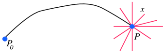
Figure 1: The lift of a coordinate neighborhood $N$ of $P$ into $\widetilde{\Sigma}$.

We choose a path $\gamma_{P}$ from $P_{0}$ to $P$ and follow it by the straight line from $P$ to $x$. Call $\gamma_{x}$ this path from $P_{0}$ to $x$. Then $x\mapsto\gamma_{x}$ is a lift of the coordinate neighborhood to a neighborhood about $\gamma_{P}$. The connection $1$-form on $P_{\chi}$ is $0$ on $(\gamma_{x},1)$ and so is $d\theta$ on $(\gamma_{x},e^{2\pi i\theta})$. Now $\tilde{f}(\gamma_{x},e^{2\pi i\theta})=(x,e^{\pi i\int_{\gamma_{x}}(\omega+\bar{\omega})}e^{2\pi i\theta})$. Hence the $1$-form on $\Sigma$ is $\frac{1}{2}(\omega+\bar{\omega})$ in the trivialization we used. With our choices the $(0,1)$ part of the connection is $\frac{1}{2}(I+iJ)(\omega+\bar{\omega})=\omega$, which we denote by $A^{0,1}$ in Section 5.

We thus have a family of $\bar{\partial}$ operators parametrized by $J(\Sigma)$, namely $\{\bar{\partial}\otimes I_{Q_{\chi}}\}_{\chi\in J(\Sigma)}$ with canonical connection on $Q_{\chi}$. When we trivialize $Q_{\chi}$ as above, $\bar{\partial}\otimes I_{Q_{\chi}}$ becomes $\bar{\partial}+\omega=\bar{\partial}+A^{0,1}$. Another trivialization would transform $\omega$ by $L_{\Omega}+\bar{\partial}\Lambda^{0}(\Sigma)$ so that if we choose a metric on $\Sigma$ and choose $H^{0,1}(\Sigma)$ as the harmonic forms of type $(0,1)$, then $\omega$ is determined up to translation by $L_{\Omega}$ as expected. The identification $\{\bar{\partial}\otimes I_{Q_{\chi}}\}_{\chi\in J(\Sigma)}$ with $\{\bar{\partial}+A^{0,1}\}_{A^{0,1}\in H^{0,1}(\Sigma)}$ works for each $\chi$ on at most a fundamental domain in $L_{\Omega}$.

With any trivialization $Q_{\chi}\simeq\Sigma\times\mathbb{C}$, the connection $1$-form $a_{\chi}$ becomes a $1$-form $A$ on $\Sigma$ which is closed because the curvature is $0$. Furthermore, $\chi(\gamma)=\exp\left(2\pi i\int_{\gamma}A\right)$ so that $A$ is determined as a closed $1$-form up to integral $1$-cocycles. Since we have not specified the trivialization, $A$ is determined only up to a gauge transformation, i.e., as an element of $H^{1}(\Sigma,\mathbb{R})/H^{1}(\Sigma,\mathbb{Z})$. We could choose $A=(A^{0,1}+A^{1,0})/2$ with $A^{0,1}$ the harmonic representative in $H^{0,1}(\Sigma)$. Choosing another representative in the coset $A^{0,1}+L_{\Omega}$ amount to choosing another trivialization of $Q_{\chi}$. In any case, $\bar{\partial}\otimes I_{Q_{\chi}}$ becomes $\bar{\partial}+A^{0,1}$.

We conclude this appendix with the following theorem about the operator $D_{A}=*i(\bar{\partial}+A^{0,1}):\Lambda^{1,0}(\Sigma)\to\Lambda^{0,0}(\Sigma)$.

Theorem B.1

Let $\chi\in J(\Sigma)$ be a character and let $A^{0,1}$ be the associated flat connection. If $\chi=1$ then $\dim\ker D_{0}=g$. If $\chi\neq 1$ then $\dim\ker D_{A}=g-1$.

Proof: Since $\ker D_{0}=H^{1,0}(\Sigma)$ we have $\dim\ker D_{0}=g$. Now the index of $D_{A}$ equals $\operatorname{Index}D_{0}=g-1$. To complete the proof of the theorem we need only show that $\dim\ker D_{A}^{*}=\dim\operatorname{coker}D_{A}=0$. But $D_{A}^{*}=\bar{\partial}+A^{0,1}:\Lambda^{0,0}(\Sigma)\to\Lambda^{0,1}(\Sigma)$ and we have shown that $\bar{\partial}+A^{0,1}$ is $\bar{\partial}:L_{\chi}\to\Lambda^{0,1}(\Sigma)\otimes L_{\chi}$, for some character $\chi$. Now $\operatorname{c}_{1}(L_{\chi})=0$ because $L_{\chi}$ is flat. So any holomorphic section of $L_{\chi}$ has no zeroes. Thus a nonvanishing holomorphic section of $L_{\chi}$ would give a holomorphic isomorphism with $\Sigma\times\mathbb{C}$ which is not possible if $\chi\neq 1$. Hence $\dim\ker D^{*}_{A}=0$.

Appendix C Holomorphic sections of the determinant line bundle

We now compute $\operatorname{c}_{1}$ of $\operatorname{DET}(\bar{\partial}\otimes I_{Q_{0}})$ and show that the space of holomorphic sections is one dimensional.

We want to compute the determinant line bundle $\operatorname{DET}(\bar{\partial}\otimes I_{Q})\to J(\Sigma)$ of the family $\{\bar{\partial}\otimes I_{Q_{\chi}}\}_{\chi\in J(\Sigma)}$. We first compute its first Chern class using Riemann-Roch or the families index theorem.

Theorem C.1

$\operatorname{c}_{1}\left(\operatorname{DET}(\bar{\partial}\otimes I_{Q})\right)$ is represented by the basic Kähler form on $J(\Sigma)$.

Proof: The Chern character of the index bundle over $J(\Sigma)$ is

$$\int_{\Sigma}\operatorname{ch}(Q)\operatorname{Todd}T(\Sigma)$$ (C.2)

where $T(\Sigma)$ is the vector bundle over $\Sigma\times J(\Sigma)$ which is $T^{1,0}(\Sigma)$ and is independent of $J(\Sigma)$. Its Todd class is $1+\operatorname{c}_{1}(T^{1,0}(\Sigma))/2$. Following convention we define $\operatorname{c}_{1}(\Sigma)=\operatorname{c}_{1}(T^{1,0}(\Sigma))$. Further $\operatorname{ch}(Q)=\sum_{n=1}^{\infty}\operatorname{c}_{1}(Q)^{n}/n!$.

Since the first Chern class of the family is given by the $2$-form term in (C.2), we want the $4$-form in the integrand which is of total degree $2$ in the $\Sigma$ direction. If we write $\operatorname{c}_{1}(Q)$ as $\mu_{2,0}+\mu_{1,1}+\mu_{0,2}$, the decomposition of $\operatorname{c}_{1}(Q)$ along $\Sigma$, $\Sigma\times J(\Sigma)$ and $J(\Sigma)$ respectively, we find the desired $4$-form to be $\frac{1}{2}\mu_{1,1}^{2}+\mu_{0,2}\mu_{2,0}+\frac{1}{2}\mu_{0,2}\operatorname{c}_{1}(\Sigma)$. Since $Q_{\chi}$ is flat, $\mu_{2,0}=\operatorname{c}_{1}(Q_{\chi})=0$; so

$$\operatorname{c}_{1}\left(\operatorname{DET}(\bar{\partial}\otimes I_{Q})\right)=\frac{1}{2}\int_{\Sigma}\left(\mu_{1,1}^{2}+\mu_{0,2}\operatorname{c}_{1}(\Sigma)\right)\;.$$

We now compute $\mu_{1,1}$ and show that $\mu_{0,2}=0$. We do so using the fact that $\operatorname{c}_{1}(Q)=\frac{1}{2\pi i}\partial\bar{\partial}\|F\|^{2}$ where $F$ is a local holomorphic section of $Q$ and $\|\bullet\|$ is the norm for the hermitian metric on $Q$.

Let $N_{P}$ be a neighborhood of $P\in\Sigma$, and let $U_{\chi}$ be a coordinate neighborhood of $\chi\in J(\Sigma)$. Because $H^{0,1}(\Sigma)$ covers $J(\Sigma)$, we can identify $U_{\chi}$ with a neighborhood of the appropriate $A^{0,1}\in H^{0,1}(\Sigma)$. In fact we can take $U_{\chi}=A^{0,1}+U_{0}$ where $U_{0}$ is a neighborhood of the origin in $H^{0,1}(\Sigma)$.

Fix a path $\gamma_{0}$ from $P_{0}$ to $P$. If $x\in N_{P}$, let $\gamma_{x}$ be the path from $P_{0}$ to $x$ which is $\gamma_{0}$ followed by the straight line from $P$ to $x$ (see Figure 1). For $(x,\omega)\in N_{P}\times U_{\chi}$ let $F(x,\omega)=\exp^{2\pi i\int_{\gamma_{x}}\omega}$. For each $\omega\in U_{\chi}$, $F$ is actually a function on the lift of $N_{P}$ to $\widetilde{\Sigma}$; it transforms correctly under $\pi_{1}(\Sigma)$ to give a local section of $Q_{\chi_{\omega}}$. We leave the reader to check that $F$ is a holomorphic section of $Q$ over $N_{P}\times U_{\chi}$.

Now $\frac{1}{2\pi i}\log\|F\|^{2}(x,\omega)=\int_{\gamma_{x}}(\omega-\bar{\omega})$ and $d_{\Sigma}$ of this expression is $(\omega-\bar{\omega})$. Hence $\frac{1}{2\pi i}\bar{\partial}_{\Sigma}\log\|F\|^{2}=\omega$ and $\frac{1}{2\pi i}\partial_{\Sigma}\log\|F\|^{2}=-\bar{\omega}$. Since $\log\|F\|^{2}$ is (real) linear in $\omega$,

$$\frac{1}{2\pi i}\left(d_{\Sigma}\log\|F\|^{2}\right)(\tau)=\int_{\gamma_{x}}(\tau-\bar{\tau})\;,$$

for $\tau\in T_{\omega}(J(\Sigma))\cong H^{0,1}(\Sigma)$. Hence

$$\frac{1}{2\pi i}\left(\bar{\partial}_{\Sigma}\log\|F\|^{2}\right)(\tau)=-\int_{\gamma_{x}}\bar{\tau}\;,$$

while

$$\frac{1}{2\pi i}\left(\partial_{\Sigma}\log\|F\|^{2}\right)(\tau)=\int_{\gamma_{x}}\tau\;.$$

Furthermore linearity implies $\partial_{J(\Sigma)}\bar{\partial}_{J(\Sigma)}\log\|F\|^{2}=0$. We conclude that $\mu_{0,2}=0$ and $\mu_{1,1}(\partial/\partial\bar{z},\tau)=\tau(\partial/\partial\bar{z})$ and $\mu_{1,1}(\partial/\partial z,\tau)=-\bar{\tau}(\partial/\partial z)$. Hence for $\tau\in T_{\omega}(J(\Sigma))$. $\mu_{1,1}(\bullet,\tau)$ is the $1$-form on $\Sigma$ equal to $(\tau-\bar{\tau})$ and the two form $\frac{1}{2}\int_{\Sigma}\mu_{1,1}^{2}$ on $J(\Sigma)$ evaluated at $\tau_{1}$, $\tau_{2}$ equals

$$\int_{\Sigma}(\tau_{1}-\bar{\tau}_{1})\wedge(\tau_{2}-\bar{\tau}_{2})=\frac{1}{2}\int_{\Sigma}\left(-\tau_{1}\wedge\bar{\tau}_{2}+\tau_{2}\wedge\bar{\tau}_{1}\right)\;.$$

Finally we recall that the metric on $J(\Sigma)$ is given by the inner product on $H^{0,1}(\Sigma)$:

$$\left\langle\tau_{2},\tau_{1}\right\rangle=\int_{\Sigma}\tau_{1}\wedge*\bar{\tau}_{2}=i\int_{\Sigma}\tau_{1}\wedge\bar{\tau}_{2}\;.$$

Thus $\frac{1}{2}\int_{\Sigma}\mu_{1,1}^{2}=\frac{i}{2}(\langle\tau_{2},\tau_{1}\rangle-\overline{\langle\tau_{2},\tau_{1}\rangle})$. Moreover, $(\langle\tau_{2},\tau_{1}\rangle-\overline{\langle\tau_{2},\tau_{1}\rangle})=-2i\omega(\tau_{1},\tau_{2})$ with $\omega$ the basic Kähler form on $J(\Sigma)$. Hence the first Chern class $\operatorname{c}_{1}\left(\operatorname{DET}(\bar{\partial}\otimes I_{Q})\right)$ of the determinant line bundle for $\{\bar{\partial}\otimes I_{Q_{\chi}}\}_{\chi\in J(\Sigma)}$ equals $\omega$.

Corollary C.3

The space of holomorphic sections of the determinant line bundle $\operatorname{DET}(\bar{\partial}\otimes I_{Q})\to J(\Sigma)$ has dimension 1.

Proof: Because $\operatorname{c}_{1}(\operatorname{DET}(\bar{\partial}\otimes I_{Q}))=\omega$, $\operatorname{DET}(\bar{\partial}\otimes I_{Q})\to J(\Sigma)$ is a positive line bundle. The Kodaira vanishing theorem applies and tell us that $\dim H^{0}(\bar{\partial}\otimes I_{Q})$ equals the Euler class of the elliptic complex

$$\Lambda^{0,q}\otimes\operatorname{DET}(\bar{\partial}\otimes I_{Q})\stackrel{{\scriptstyle\bar{\partial}\otimes I_{Q}}}{{\longrightarrow}}\Lambda^{0,q+1}\otimes\operatorname{DET}(\bar{\partial}\otimes I_{Q})$$

and is computable by Riemann-Roch. Note that $\operatorname{Todd}J(\Sigma)=1$ hence

$$\dim H^{0}(\bar{\partial}\otimes I_{Q})=\int_{J(\Sigma)}\operatorname{ch}(Q)\operatorname{Todd}J(\Sigma)=\int_{J(\Sigma)}\omega^{g}/g!=1\;.$$

References

- [1] L. Alvarez-Gaume, “Supersymmetry and the Atiyah-Singer index theorem,” Commun. Math. Phys. 90 (1983) 161.
- [2] D. Friedan and P. Windey, “Supersymmetric derivation of the Atiyah-Singer index and the chiral anomaly,” Nucl. Phys. B235 (1984) 395.
- [3] E. Witten, “Unpublished.” See M. F. Atiyah’s exposition in Astérisque 131, 1985, p. 43.
- [4] O. Alvarez, T. P. Killingback, M. Mangano, and P. Windey, “The Dirac-Ramond operator in string theory and loop space index theorems,”. Invited talk presented at the Irvine Conf. on Non- Perturbative Methods in Physics, Irvine, Calif., Jan 5-9, 1987.
- [5] O. Alvarez, T. P. Killingback, M. Mangano, and P. Windey, “String theory and loop space index theorems,” Commun. Math. Phys. 111 (1987) 1.
- [6] K. Pilch, A. N. Schellekens, and N. P. Warner, “Path integral calculation of string anomalies,” Nucl. Phys. B287 (1987) 362.
- [7] E. Witten, “Elliptic genera and quantum field theory,” Commun. Math. Phys. 109 (1987) 525.
- [8] E. Witten, “The Dirac operator in loop space,” in Elliptic Curves and Modular Forms in Algebraic Topology, P. S. Landweber, ed., Lecture Notes in Mathematics, 1326. Springer Verlag, 1988.
- [9] P. S. Landweber, ed., Elliptic Curves and Modular Forms in Algebraic Topology, Lecture Notes in Mathematics, 1326. Springer Verlag, 1988.
- [10] E. Witten, “Topological sigma models,” Commun. Math. Phys. 118 (1988) 411.
- [11] M. Atiyah, “Topological quantum field theories,” Inst. Hautes Études Sci. Publ. Math. (1988), no. 68, 175–186 (1989).
- [12] D. S. Freed and M. J. Hopkins, “On Ramond-Ramond fields and K-theory,” JHEP 05 (2000) 044, hep-th/0002027.
- [13] M. J. Hopkins and I. M. Singer, “Quadratic functions in geometry, topology and M-theory.” Unpublished.
- [14] M. F. Atiyah, “Riemann surfaces and spin structures,” Ann. Sci. École Norm. Sup. (4) 4 (1971) 47–62.
- [15] O. Alvarez, “Topological quantization and cohomology,” Commun. Math. Phys. 100 (1985) 279.
- [16] G. Moore and P. Nelson, “Anomalies in nonlinear sigma models,” Phys. Rev. Lett. 53 (1984) 1519.
- [17] G. Moore and P. Nelson, “The ætiology of sigma model anomalies,” Commun. Math. Phys. 100 (1985) 83.
- [18] D. S. Freed, “On determinant line bundles,” in Mathematical Aspects of String Theory, S. T. Yau, ed. World Scientific, 1987. Proceedings of the conference helt at University of California, San Diego July 21 – August 1, 1986.
- [19] J.-M. Bismut and D. S. Freed, “The analysis of elliptic families. I. Metrics and connections on determinant bundles,” Comm. Math. Phys. 106 (1986), no. 1, 159–176.
- [20] J.-M. Bismut and D. S. Freed, “The analysis of elliptic families. II. Dirac operators, eta invariants, and the holonomy theorem,” Comm. Math. Phys. 107 (1986), no. 1, 103–163.
- [21] W. A. Bardeen and B. Zumino, “Consistent and covariant anomalies in gauge and gravitational theories,” Nucl. Phys. B244 (1984) 421.
- [22] D. S. Freed, “Classical Chern-Simons theory. part 1,” Adv. Math. 113 (1995) 237–303, hep-th/9206021.
- [23] W. A. Bardeen, “Anomalous Ward identities in spinor field theories,” Phys. Rev. 184 (1969) 1848–1857.
- [24] K. Fujikawa, “Path integral measure for gauge invariant fermion theories,” Phys. Rev. Lett. 42 (1979) 1195.
- [25] L. Alvarez-Gaume and P. Ginsparg, “The structure of gauge and gravitational anomalies,” Ann. Phys. 161 (1985) 423.
- [26] M. F. Atiyah and I. M. Singer, “Index of elliptic operators. V,” Ann. of Math. (2) 93 (1971) 139–149.
- [27] L. Alvarez-Gaume, G. Moore, and C. Vafa, “Theta functions, modular invariance, and strings,” Commun. Math. Phys. 106 (1986) 1–40.
- [28] D. Mumford, Tata Lectures on Theta I. Birkhäuser, 1983.
- [29] J. D. Fay, Theta functions on Riemann surfaces, vol. 352 of Lecture Notes on Mathematics. Springer-Verlag, 1973.
- [30] D. Mumford, Tata Lectures on Theta II. Birkhäuser, 1984.
- [31] M. A. Kervaire and J. W. Milnor, “Groups of homotopy spheres: I,” Ann. Math. 77 (1963) 504–537.
- [32] F. Hirzebruch, T. Berger, and R. Jung, Manifolds and modular forms. Friedr. Vieweg & Sohn, Braunschweig, 1992.
- [33] P. Griffiths and J. Harris, Principles of Algebraic Geometry. Wiley, 1978.