Unruh Radiation, Holography and Boundary Cosmology

Sumit R. Das^a,b and Andrei Zelnikov^a,c,d

Yukawa Institute for Theoretical Physics

Kyoto University, Kyoto 606, JAPAN ^a

Tata Institute of Fundamental Research

Homi Bhabha Road, Mumbai 400 005 INDIA ^b

Theoretical Physics Institute, Department of Physics

University of Alberta, Edmonton AB, CANADA ^c

P.N. Lebedev Physics Institute,

Leninsky pr. 53, Moscow 117924, RUSSIA ^d

das@theory.tifr.res.in          zelnikov@phys.ualberta.ca

Abstract

A uniformly acclerated observer in anti-deSitter spacetime is known to detect thermal radiation when the acceleration exceeds a critical value. We investigate the holographic interpretation of this phenomenon. For uniformly accelerated trajectories transverse to the boundary of the $AdS$ space, the hologram is a blob which expands along the boundary. Observers on the boundary co-moving with the hologram become observers in cosmological spacetimes. For supercritical accelerations one gets a Milne universe when the holographic screen is the boundary in Poincaré coordinates, while for the boundary in hyperspherical coordinates one gets deSitter spacetimes. The presence or absence of thermality is then interpreted in terms of specific classes of observers in these cosmologies.

1 Introduction

The concrete realization of the ideas of holography [1] in terms of the $AdS-CFT$ correspondence [2] has provided a new insight into spacetime physics. According to this correspondence, all states of string theory or M-theory in an asymptotically $AdS_{m}\times S^{n}$ background can be described as states in a theory which is defined on the boundary of $AdS$ and which does not involve gravity. In particular for $m=3,5$ the boundary theory is a conventional large-N gauge theory. The vacuum of the boundary theory corresponds to a background which is purely $AdS$ while gauge invariant states are described as states of string theory defined in this background. More interestingly, a thermal state of the gauge theory is dual to a $AdS$ black hole at the same temperature [3]. This is consistent with the success of microscopic understanding of entropy and Hawking radiation of near-extremal black holes in string theory [4].

The phenomenon of Hawking radiation from Schwarzschild black holes is deeply related to Unruh radiation [5] detected by a uniformly accelerated observer in flat space, essentially because the near-horizon geometry of such black holes is Rindler space. A uniformly accelerated observer in $AdS$ spacetime would also perceive the $AdS$-invariant vacuum to be a thermal bath, provided the acceleration exceeds a critical value [6], a fact which can be proved for any field theory [7] and can be easily understood in terms of the trajectories in the global embedding spacetime. In this paper we attempt a holographic understanding of such acceleration radiation.

One of the motivations behind this work is to get some holographic insight into bulk physics as perceived by various classes of observers. The AdS/CFT correspondence has given a rather satisfactory description of the bulk physics for a certain class of observers, e.g. for observers who are stationary outside a black hole. To understand black hole complementarity, however, we need to compare this with the description of bulk physics from the viewpoint of other observers, like those freely falling into a black hole. Some of these interesting problems are quite general and do not depend on presence of a black hole. In this paper our analysis is focused on observer dependent properties of quantum fields in $AdS$ spacetime and their holographic interpretation on the boundary. We hope that it will provide some insight into the holographic description of physics for an interesting class of accelerated observers.

Consider a geodesic in the bulk of $AdS$ which is entirely transverse to the boundary. As expected from the IR/UV relationship, the “image” of this in the boundary theory is a blob [8], or rather a “bubble” [9] which expands in the longitudinal directions along the boundary. The size of the image at any given time is related to the distance of the object from the boundary. When we have a uniformly accelerated trajectory in the bulk we, of course, have a similar physics. The nature of the expanding image depends on whether or not the acceleration exceeds a critical bound. We will find that observers according to whom the holographic image is time-independent are like observers in cosmological spacetimes. When the accleration exceeds the critical value, such observers preceive the vacuum as a thermal state, while for subcritical or critical acclerations they dont.

The nature of the cosmology we obtain depends on the particular coordinates in $AdS$ used to define a boundary. We will need to work not really on the boundary, but at a small but finite distance away from the boundary. This implies that the holographic theory has an UV cutoff. We will nevertheless continue to refer to the holographic screen as the “boundary”. For example, on the Poincaré boundary, which is flat, images of observers with a supercritical acceleration in the bulk, look like observers who use the conformal time in an expanding Milne universe. According to them the image of the accelerating bulk object is time independent. These boundary observers do not cover the complete Poincaré boundary and perceive the invariant vacuum as a thermal state [10]. The picture looks different in the case of observers with critical or subcritical accelerations. These map on to boundary observers whose coordinate systems cover the entire Poincaré boundary. On the other hand, the boundary defined in a coordinate system in $AdS_{d+1}$ which is similar to the standard spherical coordinate system on a sphere and may be obtained from it by analytical continuation ( we call these “hyperspherical coordinates”) is $d$ dimensional deSitter spacetime. Now subcritical acclerations correspond to the choice of global time in $dS_{d}$. Critical acclerations correspond to choice of the conformal time in the extension of the steady state universe which covers the entire $dS_{d}$ boundary. Supercritical accelerations correspond to the time in the $dS_{d}$ coordinate system in which the metric is time-independent. For well known reasons the last class of observers detect a thermal bath [11, 10].

The appearance of a cosmological interpretation of Unruh radiation in the bulk is intruiging. This is similar to the microscopic interpretation of the deSitter entropy in two dimensions in [12]. Here one has a physical brane in the bulk theory which is also the holographic screen. Its location is determined dynamically by the brane tension. Consequently, the holographic theory has dynamical gravity [13, 12] as in brane world models [14]. In hyperspherical coordinates, the entropy of the deSitter spacetime on the screen is understood as entaglement entropy as in theories of induced gravity [15]. From our point of view, this happens because stationary observers on the screen are bulk accelerated observers with supercritical acceleration which are moving along the screen. In our work, we have a fixed holographic screen and we look at objects in the bulk which are away from the screen with no motion along it. Nevertheless, examining their holograms lead to similar connections with cosmological spacetimes - not only for screens placed near the boundary in hyperspherical coordinates but for other coordinates as well. This circle of ideas is also somewhat related to the observation of [6] that thermal properties of spacetimes with genuine gravity, like black holes or deSitter spaces can be in fact derived from the thermal properties of acclerated observers in global embeddings spacetimes which can be flat. This latter observation, however, does not use any holographic correspondence.

In Section 2 we give the definitions of the various coordinate systems in $AdS_{d+1}$ which are used in the paper. In Section 3 we derive an equation which describes the motion of a general uniformly accelerated object in $AdS$ space and find all solutions to obtain three classes. In Section 4 we compute the one point functions in the various boundary theories for $AdS_{3}$ which provide holograms of such acclerated objects when they couple to some massless scalar field in the bulk. In Section 5 we give the boundary interpretation of presence or absence of thermal behavior as perceived by bulk observers moving along those trajectories. The various cosmolgies appear here. In Section 6 we discuss generalizations to higher dimensions and argue that the connection with boundary cosmologies is general. Section 7 contains conclusions and comments. Appendix I contains details of the various coordinate systems. Appendix II contains the details of the calculation of the formulae used in Section 4.

2 Coordinate Systems in $AdS_{d+1}$

We will consider four classes of coordinate systems in $AdS_{d+1}$. These describe different ways of choosing $AdS_{d+1}$ as a hyperbolic surface in $d+2$ dimensional flat space with two timelike coordinates. The details of the embeddings are given in the Appendix I.

2.1 Global Coordinates

The global coordinate system has a time $\tau$ which has a finite range $0<\tau<2\pi$. However very often one considers a covering space with an infinite range by attaching identical copies. The spatial coordinates include a radial variable $\nu,0<\nu<\pi/2$, and $(d-1)$ other angles $\phi,\theta_{i},i=1,\cdots d-2$ with ranges $0<\phi,\theta_{i}<\pi$ for $i=2,\cdots(d-3)$ and $0<\theta_{d-2}<2\pi$. The metric is then given by

$$ds^{2}=\sec^{2}\nu[-d\tau^{2}+d\nu^{2}+\sin^{2}\nu(d\phi^{2}+\sin^{2}\phi d\Omega_{d-2}^{2})].$$ (1)

The boundary is at $\nu=\pi/2$ in these global coordinates. Surfaces of constant $\nu=\nu_{B}$ have spatial sections which are $S^{d-1}$. When $\nu_{B}$ is close to, but less than ${\pi\over 2}$ the induced metric is

$$ds_{gIn}^{2}=\sec^{2}\nu_{B}[-d\tau^{2}+\sin^{2}\nu(d\phi^{2}+\sin^{2}\phi d\Omega_{d-2}^{2})].$$ (2)

The metric of the boundary theory is obtained by removing the overall factor of $\sec^{2}\nu_{B}$ from (2).

2.2 Poincaré Coordinates

The time in Poincaré coordinates has infinite range $-\infty<t<\infty$ and the spatial coordinates include radial variables $r,z$ with a range $0<r,z<\infty$ and $d-2$ angles on a $S^{d-2}$. These are denoted by $\theta_{i},i=1,\cdots d-2$ and have the usual ranges $0<\theta_{i}<\pi$ for $i=2,\cdots(d-3)$ and $0<\theta_{d-2}<2\pi$. These angles $\theta_{i}$ are common with the corresponding angles in the global coordinate system. The metric is now

$$ds^{2}={1\over z^{2}}[-dt^{2}+dz^{2}+dr^{2}+r^{2}d\Omega^{2}_{d-2}].$$ (3)

The Poincaré system does not cover the entire $AdS$ spacetime. For a set of static observers $~{}\{z,r,\theta_{i}\}={\mathrm{c}onst}~{}$ there is a horizon at $z=\infty$.

The Poincaré boundary is at $z=0$. Constant $z=z_{B}$ surfaces are flat, with induced metric

$$ds_{PIn}^{2}={1\over z_{B}^{2}}[-dt^{2}+dr^{2}+r^{2}d\Omega^{2}_{d-2}].$$ (4)

The boundary metric is obtained by removing the overall factor ${1\over z_{B}^{2}}$.

2.3 “BTZ” Coordinates

The third coordinate system we will use will be called “BTZ” coordinates, since this is a natural extension of the BTZ coordinates for $d=2$. The time $\eta$ has infinite range, $-\infty<\eta<\infty$. There is a radial variable $\rho$ with $1<\rho<\infty$ and another noncompact coordinate $\psi$ with $0<\psi<\infty$ and in addition the same $d-2$ angles $\theta_{i}$ as in the global and Poincaré systems. The metric is now

$$ds^{2}=-(\rho^{2}-1)d\eta^{2}+{d\rho^{2}\over(\rho^{2}-1)}+\rho^{2}[d\psi^{2}+\sinh^{2}\psi d\Omega_{d-2}^{2}].$$ (5)

These coordinates also do not cover the entire $AdS$ spacetime and static observers see horizons at $\rho^{2}=1$.

The boundary is at $\rho=\infty$. Finite $\rho=\rho_{B}$ surfaces have spatial sections which are hyperbolic spaces in $(d-1)$ dimensions. For large $\rho_{B}$ the induced metric is

$$ds^{2}_{BTZIn}=\rho_{B}^{2}[-d\eta^{2}+d\psi^{2}+\sinh^{2}\psi d\Omega_{d-2}^{2}].$$ (6)

The boundary metric is (6) divided by the factor $\rho_{B}^{2}$.

2.4 Hyperspherical coordinates

These coordinates are obtained from analytic continuations of standard polar coordinates on a $S^{d+1}$. They include a time which is in fact identical to the time $\eta$ in BTZ coordinates, a radial variable $\mu$ with $0<\mu<\infty$, an angle $\theta$ with range $0<\theta<\pi$ and the standard set of $d-2$ angles $\theta_{i}$ which are identical to the above. The metric is given by

$$ds^{2}=-\sinh^{2}\mu~{}\sin^{2}\theta d\eta^{2}+d\mu^{2}+\sinh^{2}\mu~{}d\theta^{2}+\sinh^{2}\mu\cos^{2}\theta d\Omega^{2}_{d-2}.$$ (7)

Like BTZ coordinates, these do not cover the entire $AdS$ spacetime. Once again, static observers see a horizon at $\mu=0$.

The boundary is at $\mu=\infty$. Any finite $\mu=\mu_{B}$ surface is a $d$-dimensional deSitter space with the metric

$$ds_{HIn}^{2}=\sinh^{2}\mu_{B}(-\sin^{2}\theta d\eta^{2}+d\theta^{2}+\cos^{2}\theta d\Omega^{2}_{d-2}),$$ (8)

with a constant Ricci scalar ${6/\sinh^{2}\mu_{B}}$. Once again the boundary metric is obtained by removing the overall factor. The Ricci scalar of the boundary metric is thus $6$.

3 Accelerated Trajectories

Consider a trajectory specified by the following equations in Poincaré coordinates

$$z=z(\lambda)~{}~{}~{}~{}~{}t=t(\lambda)~{}~{}~{}~{}~{}~{}r=0,$$ (9)

where $\lambda$ denotes the proper time. The components of the velocity may be then written as

$$u^{t}(\lambda) = {dt\over d\lambda}=z(\lambda)\cosh\gamma(\lambda),$$

$$u^{z}(\lambda) = {dz\over d\lambda}=z(\lambda)\sinh\gamma(\lambda),$$ (10)

with all other components equal to zero. We have written $u^{t},u^{z}$ in a way which automatically satisfies the requirement $g_{\alpha\beta}u^{\alpha}u^{\beta}=-1$. The nonzero components of an acceleration vector are

$$a^{t} = {du^{t}\over d\lambda}-{2\over z}u^{t}u^{z},$$

$$a^{z} = {du^{z}\over d\lambda}-{1\over z}[(u^{t})^{2}+(u^{z})^{2}].$$ (11)

3.1 Uniform Accceleration

Now we derive a differential equation for $\gamma(\lambda)$ such that the proper acceleration is constant along the trajectory. This means that

$$g_{\alpha\beta}a^{\alpha}a^{\beta}={1\over z^{2}}[(a^{z})^{2}-(a^{t})^{2}]=a^{2}.$$ (12)

Together with the relation $g_{\alpha\beta}u^{\alpha}a^{\beta}=0$ this implies that we can write

$$a^{t}=a~{}z(\lambda)~{}\sin\gamma(\lambda),~{}~{}~{}~{}~{}~{}a^{z}=a~{}z(\lambda)~{}\cos\gamma(\lambda).$$ (13)

Substituting this in any of the equations in (11) we easily get the following differential equation for $\gamma(\lambda)$

$${d\gamma\over d\lambda}=\cosh\gamma+a.$$ (14)

This equation can be easily solved.

1. In the first solution the right hand side of (14) vanishes,

   $$\cosh\gamma+a=0.$$ (15)

   which is possible only if $a^{2}\geq 1$. $\gamma$ is thus a constant along the trajectory. It is trivial to solve for $z(\lambda)$ and $t(\lambda)$. For $a^{2}>1$ we have

   $$z(\lambda) = A~{}e^{\pm{\sqrt{a^{2}-1}}~{}\lambda},$$

   $$t(\lambda) = \pm{a\over{\sqrt{a^{2}-1}}}A~{}e^{\pm{\sqrt{a^{2}-1}}~{}\lambda},$$ (16)

   The $\pm$ sign corresponds to the direction of $t$. We can choose this to be lower sign to get for the trajectory

   $$t={a\over{\sqrt{a^{2}-1}}}~{}z.$$ (17)

   Different values of the integration constant $A$ lead to trajectories which are related by simultaneous rescalings of $z$ and $t$, which is an isometry of the spacetime . The final equation (17), of course, does not depend on this choice.

   When $a=-1$ we have $\gamma=0$ along the trajectory. It follows from (10) that these trajectories are simply $z={\mathrm{c}onst}$.

2. The second solution has nonvanishing ${d\gamma\over d\lambda}$. Using (14) and the definitions of $u^{\alpha}(\lambda)$ we can now easily solve for $z$ and $t$ as functions of $\gamma$

   $$z = A(\cosh\gamma+a),$$

   $$t = A\sinh\gamma.$$ (18)

   so that we have the trajectory

   $$(z-aA)^{2}-t^{2}=A^{2}.$$ (19)

   The solution for $\gamma(\lambda)$ now depends on whether $a^{2}>1,~{}a^{2}=1$ or $a^{2}<1$. For $a^{2}>1$ we have

   $$\cosh\gamma={a\cosh[{\sqrt{a^{2}-1}}~{}(\lambda-\lambda_{0})]-1\over a-\cosh[{\sqrt{a^{2}-1}}~{}(\lambda-\lambda_{0})]}~{}~{}~{}~{}~{}(a^{2}>1),$$ (20)

   When $a^{2}=1$ we get

   $$\coth(\gamma/2)=-(\lambda-\lambda_{0})~{}~{}~{}~{}~{}(a^{2}=1),$$ (21)

   while for $a^{2}<1$ we have

   $$\cosh\gamma={a\cos[{\sqrt{1-a^{2}}}~{}(\lambda-\lambda_{0})]-1\over a-\cos[{\sqrt{1-a^{2}}}~{}(\lambda-\lambda_{0})]}~{}~{}~{}~{}~{}(a^{2}<1).$$ (22)

For $a^{2}\geq 1$ the trajectories of the second type can be in fact related to those of the first type by isometries of the metric. For $a^{2}>1$ we first transform to coordinates $(t^{\prime},z^{\prime},r^{\prime},\theta_{i})$ defined as

$$U={t^{\prime}\over z^{\prime}}, V={1\over 2z^{\prime}}[1+((r^{\prime})^{2}+(z^{\prime})^{2}-(t^{\prime})^{2})],$$ (23)

$$W_{1}={1\over 2z^{\prime}}[1-(r^{\prime})^{2}+(z^{\prime})^{2}-(t^{\prime})^{2})],$$

$$W_{2}={r^{\prime}\over z^{\prime}}\cos\theta_{1}, \cdots W_{d}={r^{\prime}\over z^{\prime}}\sin\theta_{1}\sin\theta_{2}\cdots\sin\theta_{d-2}.$$

This is clearly an isometry since this involves just interchange of $U$ and $V$ in (109). Defining

$$a={\rho_{0}\over{\sqrt{\rho_{0}^{2}-1}}},$$ (24)

the trajectory (17) is simply

$$t=\rho_{0}z,~{}~{}r=0~{}~{}~{}~{}~{}~{}{\rm i.e.}~{}~{}~{}V=\rho_{0}~{}~{}W_{n}=0~{}~{}(n>1).$$ (25)

Then in terms of the primed coordinates this becomes

$$(z^{\prime}-\rho_{0})^{2}-(t^{\prime})^{2}=\rho_{0}^{2}-1~{}~{}~{}~{}~{}r^{\prime}=0.$$ (26)

We then make a simultaneous rescaling of $z^{\prime}$ and $t^{\prime}$

$${\bar{z}}={A\over{\sqrt{\rho_{0}^{2}-1}}}z^{\prime},~{}~{}~{}~{}~{}~{}~{}{\bar{t}}={A\over{\sqrt{\rho_{0}^{2}-1}}}t^{\prime},$$ (27)

together with a similar rescling of $r$, which is also an isometry. The trajectory now takes the form

$$({\bar{z}}-aA)^{2}-{\bar{t}}^{2}=A^{2},$$

which is identical to (19).

Similarly for $a=-1$ the trajectory is given by

$${1\over z_{0}}=U+W_{1},~{}~{}~{}~{}~{}~{}~{}~{}r=0$$

which becomes

$$(z^{\prime}+{1\over z_{0}})^{2}-(t^{\prime}+1)^{2}=({1\over z_{0}})^{2}.$$

After performing a shift $t^{\prime}\rightarrow t^{\prime}+1$ and a simultaneous rescaling of $t^{\prime}$ and $z^{\prime}$ the trajectory becomes identical to (19) with $a=-1$ (see Fig.(1)).

We therefore need to consider only three classes of trajectories

$$(z+\xi_{0})^{2}-t^{2} = (1+\xi_{0}^{2})~{}~{}~{}~{}~{}~{}~{}~{}(a^{2}={\xi_{0}^{2}\over\xi_{0}^{2}+1}<1),$$ (28)

$$z = z_{0}~{}~{}~{}~{}~{}~{}~{}~{}~{}~{}~{}~{}~{}~{}~{}~{}~{}(a=-1),$$ (29)

$$t = \rho_{0}~{}z~{}~{}~{}~{}~{}~{}~{}~{}~{}~{}(a^{2}={\rho_{0}^{2}\over\rho_{0}^{2}-1}>1),$$ (30)

where the first trajectory (28) was obtained from (19) by choosing $A$ suitably.

Using the definitions of various coordinate systems in the previous section, it is now easy to see that (30) corresponds to a constant value of $\rho=\rho_{0}$ with $\psi=0$ in the BTZ coordinate system (see Fig.(1)), or equivalently $\mu=\mu_{0}=\cosh^{-1}\rho_{0}$ with $\theta=\pi/2$ in the hyperspherical coordinate system. Similarly, (29) corresponds to a constant value of $z=z_{0}$ in the Poincaré coordinate system and (28) corresponds to a constant value of $\nu=\nu_{0}$ in the global coordinate system where $\tan\nu_{0}=\xi_{0}$.

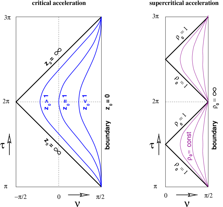
Figure 1: Left picture: The trajectories corresponding to the critical accleleration $a=-1$. Right picture: The trajectories with supercritical acceleration $a^{2}>1$.

We have performed the analysis of accelerated trajectories using the Poincaré coordinate system. However the analysis can be redone in any other coordinate system. Even though the Poincaré, BTZ and hyperspherical coordinate systems do not cover the entire $AdS$ spacetime the basic differential equation (14) can be easily transformed to the global coordinate system and solved. The final result is, of course, the same and we have the three basic classes of trajectories as listed above. For example, in global coordinates these trajectories become

$$\nu=\nu_{0} ~{}~{}~{}~{}(a^{2}<1),$$ (31)

$$\sec\nu\cos\tau\pm\tan\nu={1\over z_{0}} ~{}~{}~{}~{}(a=-1),$$

$$\sec\nu\sin\tau=\rho_{0} ~{}~{}~{}~{}(a^{2}>1).$$

All these trajectories have $\sin\phi=0$. Starting from $\phi=0$ The $\pm$ sign in the second equation refers to the sides of a section with $\sin\phi=0$. Since this trajectory can pass from the side with $\phi=0$ to the side which has $\phi=\pi$, it is conveninent to imagine that the sign of $\nu$ is reversed in this latter side. This explains why we consider the range $-{\pi/2}<\nu<\pi/2$ in Figure (1).

3.2 Unruh radiation

In flat space, any unformly accelerated observer perceives the Minkowski vacuum as a thermal state. In $AdS$ space, however, among the three classes of unform acceleration, only observers which follow the trajectory (30) or those obtained from this by isometries will perceive the $AdS$ vacuum as a thermal state [6]. A nice way to see this is to consider the corresponding trajectories in the $d+2$ dimensional space $(U,V,W_{i})$ in which $AdS_{d+1}$ is embedded as a hyperboloid. Only those trajectories with $a^{2}>1$ have a real acceleration in this embedding spacetime, and the corresponding temperature can be read off from the usual Unruh formula [6]. Another way to see this is to consider the horizons perceived by the class of accelerated observers and calculate the surface gravity. This calculation can be done entirely in global coordinates. However, as in the case of spacetimes with bifurcate Killing horizons (see [7]), it is easier done in appropriate coordinates where the time is chosen to be along the Killing vector which becomes null at the horizon. The answer is valid for arbitrary interacting fields and is, of course, coordinate invariant.

Thus for $a^{2}=1$ trajectories the horizon is simply at $z=\infty$ (in Poincaré coordinates), where the Killing vector $k=z_{0}{\partial\over\partial t}$ becomes null. We assume the Killing vector to be normalized $k^{\epsilon}k_{\epsilon}=-1~{}|_{z=z_{0}}$ at the location of the observer. The surface gravity for the horizon reads

$$\kappa^{2}=-{1\over 2}\nabla^{\alpha}k^{\beta}\nabla_{\alpha}k_{\beta}|_{z=\infty}={z_{0}^{2}\over z^{2}}|_{z=\infty}=0.$$ (32)

This implies that the Unruh temperature vanishes.

For the $a^{2}>1$ trajectories are specified by constant $\rho=\rho_{0}$ in the BTZ coordinates and the horizon is at $\rho=1$. Here the Killing vector $k={1\over\sqrt{\rho_{0}^{2}-1}}{\partial\over\partial\eta}$ becomes null and the surface gravity is

$$\kappa^{2}=-{1\over 2}\nabla^{\alpha}k^{\beta}\nabla_{\alpha}k_{\beta}|_{\rho=1}={\rho^{2}\over\rho_{0}^{2}-1}|_{\rho=1}={1\over\rho_{0}^{2}-1}\hskip 28.45274ptk^{\epsilon}k_{\epsilon}=-1~{}|_{\rho=\rho_{0}}.$$ (33)

The local temperature measured by an observer at $\rho=\rho_{o}$ then reads

$$T_{local}={1\over 2\pi{\sqrt{\rho_{0}^{2}-1}}}.$$ (34)

This implies that it is just red-shifted Unruh temperature

$$T_{U}={1\over 2\pi},$$ (35)

measured at infinity.

For $a^{2}<1$ the trajectories have constant $\nu$ in global coordinates and there is no horizon and, hence, no temperature.

4 Holograms of the trajectories in $AdS_{3}$

The above trajectories in the bulk have holograms on the boundary. The profile of the hologram may be obtained as follows. Imagine that we have a source of some supergravity field which is moving along some trajectory in the bulk, specified by $Y^{\alpha}(\lambda)$. The one point function of the operator of the boundary theory which is dual to this field evaluated in a state corresponding to the motion of the source is then obtained by evaluating the value of this field on the boundary and then integrating over the world-line of the source [8, 9].

For simplicity we will consider a source which is coupled to a minimally coupled massless scalar field in the $AdS$ spacetime. We therefore need to calculate the scalar Green’s function between a point on the trajectory $Y^{\alpha}(\lambda)$ and a point in the bulk $X^{\alpha}$ and integrate this over the trajectory. Finally we have to take the point $X$ to the boundary. In this section we will perform this computation for the case of $AdS_{3}$. Generalization to other $AdS_{d+1}$ and to sources of other supergravity fields should be quite similar in spirit.

The hologram would of course depend on the specific boundary which is chosen. We will choose three different boundaries, (i) the boundary defined in Poincaré coordinates defined by $z=0$ , (ii) the boundary in global coordinates defined by $\nu={\pi\over 2}$ and (iii) the boundary defined in hyperspherical coordinates at $\mu=\infty$. The one point functions would be then results in the corresponding boundary theory. In each case we will consider the holographic screen a little away from the boundary, i.e. for small but finite $z$, for $\nu$ close to, but less than ${\pi\over 2}$ and for $\mu$ large but finite. As is well known from the IR/UV correspondence, this corresponds to a boundary theory with an ultraviolet cutoff.

In $AdS_{3}$ the scalar Green’s function for a massless scalar field is given by [9]

$$G(X,Y) = -{1\over 2\pi}\cot(v)~{}~{}~{}~{}~{}-1<\cos v<1,$$ (36)

$$= 0\hskip 93.89418pt{\rm otherwise},$$

where $v$ is the timelike geodesic distance between the point $X$ and $Y$.

In global coordinate system defined in (105) the geodesic distance is given by

$$\cos(v)=\sec\nu~{}\sec\nu^{\prime}~{}\cos(\tau-\tau^{\prime})-\tan\nu~{}\tan\nu^{\prime}~{}\cos(\phi-\phi^{\prime}),$$ (37)

where we have labelled $X=(\tau,\nu,\phi)$ and $Y=(\tau^{\prime},\nu^{\prime},\phi^{\prime})$.

In Poincaré coordinate system defined in (109) one has

$$\cos(v)=1+{(r-r^{\prime})^{2}+(z-z^{\prime})^{2}-(t-t^{\prime})^{2}\over 2zz^{\prime}},$$ (38)

where $X=(t,z,r)$ and $Y=(t^{\prime},z^{\prime},r^{\prime})$.

In the BTZ coordinate system defined in (113) one has

$$\cos(v)=\rho\rho^{\prime}\cosh(\psi-\psi^{\prime})-{\sqrt{(\rho^{2}-1)(\rho^{\prime 2}-1)}}~{}\cosh(\eta-\eta^{\prime}),$$ (39)

where $X=(\eta,\rho,\psi)$ and $Y=(\eta^{\prime},\rho^{\prime},\psi^{\prime})$.

Finally in the hyperspherical coordinate system, with $X=(\eta,\mu,\theta)$ and $Y=(\eta^{\prime},\mu^{\prime},\theta^{\prime})$

$$\cos(v)=\cosh\mu\cosh\mu^{\prime}-\sinh\mu\sinh\mu^{\prime}[\sin\theta\sin\theta^{\prime}\cos(\eta-\eta^{\prime})-\cos\theta\cos\theta^{\prime}].$$ (40)

The value of the scalar field at the location $X^{\alpha}$ in the bulk due to a source moving along $Y^{\alpha}=Y^{\alpha}(\lambda)$ is then given by [9]

$$\Phi(X)=\int d\lambda G(X,Y(\lambda)),$$ (41)

where we substitute for the specific form of the trajectory $Y^{\alpha}(\lambda)$ and $\lambda$ denotes the proper time. The answer is of course independent of the coordinate system used to do the calculation. However the one point function for a specific boundary theory

$$<{\cal O}>\sim\Phi(X)|_{boundary},$$ (42)

depends on the coordinates used to define the boundary. The transformation between different coordinate systems become conformal transformations when restricted to the boundary. The one point function for different boundary theories can then be related by transforming $<{\cal O}>$ according to the standard rules determined by its conformal weight.

Strictly speaking, one has to divide the right side of (42) by the radial part of the normalizable wave function evaluated on the boundary [2, 8, 16]. The latter is a cutoff factor which is consistent with the correct conformal weight of ${\cal O}$. However, in the following we will retain this cutoff factor in the formulae for reasons which will become clear later.

The strategy to calculate $\Phi(X)$ is to first use a coordinate system which is best suited for the particular kind of acceleration. Since subcritical accelerations are described in global coordinates by $\nu=\nu_{0}$ we use global coordinates for this computation. Similarly for the critical and supercritical accelerations we use the Poincaré and BTZ coordinates respectively. Once this is done we can transform to any coordinate system we like. This latter system is chosen according to which boundary we are considering. We then take the limit of $\Phi(X)$ for the appropriate boundary to extract the one point function.

In the following we outline the derivation of boundary one point functions for Poincaré, global and hyperspherical boundaries. Details of the calculation of the field are given in Appendix II.

4.1 Poincaré Boundary

The Poincaré boundary is at $z=z_{B}\rightarrow 0$ and we will need $\Phi(X)$ in the Poincaré coordinate system.

4.1.1 Subcritical Accelerations, $a^{2}<1$

First consider trajectories given by (28) which have accelerations $a^{2}<1$. Since these correspond to constant values of $\nu=\nu_{0}$ it is most conveninent to write down the Green’s function and the field $\Phi(X)$ in global coordinates. The result is in the Appendix II, equation (124). We then transform to Poincaré coordinates. The result is

$$\Phi(X)={2z\sec\nu_{0}\over 2\pi}\int_{0}^{\pi}dv~{}{\cos v\over[\sec^{2}\nu_{0}(4t^{2}+(1+s)^{2})-(2z\cos v+\tan\nu_{0}(1-s))^{2}]^{1/2}},$$ (43)

where

$$s=r^{2}+z^{2}-t^{2}.$$ (44)

The one point function is then given by

$$<{\cal O}>^{a^{2}<1}_{Poincare}=\Phi(X)|_{z=z_{B}\rightarrow 0}.$$ (45)

The leading answer vanishes and one has to evaluate the first subleading (in $z_{B}$) contribution. The answer is

$$<{\cal O}>^{a^{2}<1}_{Poincare}=z_{B}^{2}{\sin\nu_{0}\over\cos^{2}\nu_{0}}{(1-(r^{2}-t^{2}))\over[4t^{2}+(1+(r^{2}-t^{2}))^{2}+4r^{2}\tan^{2}\nu_{0}]^{3/2}}$$ (46)

Note that there is an overall factor $z_{B}^{2}$ in the expression, and $z_{B}\rightarrow 0$. From the UV/IR connection $z_{B}$ appears as a (position space) UV cutoff in the boundary theory, as is evident from the form of the metric restricted to the boundary. The power of $z_{B}$ in (46) reflects the fact that ${\cal O}$, being dual to a massless scalar field in the bulk, is a $(1,1)$ operator on the boundary.

4.1.2 Critical Acceleration

For the trajectory (29) with critical acceleration one has $z^{\prime}=z_{0}$ in the Poincaré system. Therefore we do the calculation in this coordinate system. The result is equation (128) in Appendix II which we rewrite here

$$\Phi(X)={z\over 2\pi}\int_{0}^{\pi}dv~{}{\cos v\over[r^{2}+z^{2}+z_{0}^{2}-2zz_{0}\cos v]^{1/2}}.$$ (47)

This one point function can be read off directly by considering the leading contribution when $z=z_{B}\rightarrow 0$ :

$$<{\cal O}>^{a^{2}=1}_{Poincare}={z_{B}^{2}z_{0}\over 4(r^{2}+z_{0}^{2})^{3/2}}.$$ (48)

As expected, the one point function is a constant in Poincaré time and the correct factor of cutoff appears.

4.1.3 Supercritical Acceleration

Finally we consider the case of $a^{2}>1$ given by the trajectory (30) $\rho^{\prime}=\rho_{0}$ in BTZ coordinates. Therefore we first do the calculation in BTZ coordinates. The result is (134) in Appendix II. In Poincaré coordinates this becomes

$$\Phi(X)={z{\sqrt{\rho_{0}^{2}-1}}\over 2\pi}\int_{0}^{\pi}dv~{}{\cos v\over[(\rho_{0}t-z\cos v)^{2}+(\rho_{0}^{2}-1)(r^{2}+z^{2}-t^{2})]^{1/2}},$$ (49)

which leads to the one point function

$$<{\cal O}>^{a^{2}>1}_{Poincare}={z_{B}^{2}\rho_{0}{\sqrt{\rho_{0}^{2}-1}}\over 4}{t\over[(\rho_{0}^{2}-1)r^{2}+t^{2}]^{3/2}}.$$ (50)

4.2 Global Boundary

The one point functions in the boundary theory defined on the boundary in global coordinates, $\nu=\nu_{B}\rightarrow{\pi\over 2}$ can be obtained by entirely similar methods. For all cases we write down the field $\Phi(X)$ in global coordinates and evaluate the leading nonzero contribution in the limit $\nu_{B}\rightarrow{\pi\over 2}$.

4.2.1 Subcritical Accelerations

For $a^{2}<1$ the calculation is trivial since the trajectories are those of constant values of $\nu^{\prime}=\nu_{0}$. The one point function may be obtained by simply taking the limit of $\Phi(X)$ in (124) as $\nu\rightarrow{\pi\over 2}$. The result is

$$<{\cal O}>^{a^{2}<1}_{global}={\cos^{2}\nu_{B}\over 4}{\sin\nu_{0}\over\cos^{2}\nu_{0}}{\cos\phi\over[1+\tan^{2}\nu_{0}\sin^{2}\phi]^{3/2}},$$ (51)

which is of course constant in global time. The overall factor of $\cos^{2}\nu_{B}$ is the UV cutoff factor as is evident from the form of the metric and its appearance is consistent with the dimension of the operator ${\cal O}$.

4.2.2 Critical Acceleration

For $a^{2}=1$, the field (128) has to be first transformed into global coordinates. The result is

$$\Phi(X)={\cos\nu\over 2\pi}\int_{0}^{\pi}dv~{}{\cos v\over\Delta^{1/2}},$$ (52)

where

$$\Delta=(\sin^{2}\nu\sin^{2}\phi+\cos^{2}\nu)+z_{0}^{2}(\cos\tau+\sin\nu\cos\phi)^{2}-2z_{0}\cos\nu\cos v~{}(\cos\tau+\sin\nu\cos\phi).$$ (53)

This leads to the one point function

$$<{\cal O}>^{a^{2}=1}_{global}={z_{0}\cos^{2}\nu_{B}\over 4}~{}{\cos\tau+\cos\phi\over[\sin^{2}\phi+z_{0}^{2}(\cos\tau+\cos\phi)^{2}]^{3/2}}.$$ (54)

This is now a nontrivial function of the time $\tau$ on the global boundary.

4.2.3 Supercritical Acceleration

The field $\Phi(X)$ (134) is, in terms of global coordinates,

$$\Phi(X)={\cos\nu{\sqrt{\rho_{0}^{2}-1}}\over 2\pi}\int_{0}^{\pi}dv~{}{\cos v\over[(\rho_{0}\sin\tau-\cos\nu\cos v)^{2}-(\rho_{0}^{2}-1)(\sin^{2}\nu\cos^{2}\phi-\cos^{2}\tau)]^{1/2}},$$ (55)

which leads to the one point function

$$<{\cal O}>^{a^{2}>1}_{global}={\cos^{2}\nu_{B}~{}\rho_{0}{\sqrt{\rho_{0}^{2}-1}}\over 4}{\sin\tau\over[(\rho_{0}^{2}-1)\sin^{2}\phi+\sin^{2}\tau]^{3/2}}.$$ (56)

4.3 Boundary in Hyperspherical coordinates

In hyperspherical coordinates the boundary is at $\mu=\mu_{B}$ and we have to consider the limit $\mu_{B}\rightarrow\infty$.

4.3.1 Subcritical Accelerations

For $a^{2}<1$ we first need to write the field $\Phi(X)$ in (121) at arbitrary $X$ in the hyperspherical coordinates. The result is

$$\Phi(X)={\sec\nu_{0}\over 2\pi}\int_{0}^{\pi}dv{\cos v\over\Sigma^{1/2}},$$ (57)

where

$$\Sigma=\sec^{2}\nu_{0}(\sinh^{2}\mu\sin^{2}\theta\sinh^{2}\eta+\cosh^{2}\mu)-(\cos v+\sinh\mu\sin\theta\cosh\eta\tan\nu_{0})^{2}.$$ (58)

The one point function is obtained by evaluating the leading nonzero contrinution as we take $\mu=\mu_{B}\rightarrow\infty$

$$<{\cal O}>^{a^{2}<1}_{hyperspherical}={1\over 4\sinh^{2}\mu_{B}}{\sin\nu_{0}\over\cos^{2}\nu_{0}}{\sin\theta\sinh\eta\over[\sec^{2}\nu_{0}+\sin^{2}\theta\sinh^{2}\eta-\tan^{2}\nu_{0}\sin^{2}\theta]^{3/2}}.$$ (59)

4.3.2 Critical Acceleration

The field $\Phi(X)$ in (125) becomes in hyperspherical coordinates

$$\Phi(X)={e^{-\eta}\over 2\pi}\int_{0}^{\pi}{\cos v\over{\tilde{\Sigma}}^{1/2}},$$ (60)

where

$${\tilde{\Sigma}}=e^{-2\eta}(1+\sinh^{2}\mu\cos^{2}\theta)+z_{0}^{2}\sinh^{2}\mu\sin^{2}\theta-2z_{0}e^{-\eta}\sinh\mu\sin\theta\cos v.$$ (61)

The result for the one point function is

$$<{\cal O}>^{a^{2}=1}_{hyperspherical}={z_{0}\over 4\sinh^{2}\mu_{B}}{\sin\theta~{}e^{-2\eta}\over[z_{0}^{2}\sin^{2}\theta+e^{-2\eta}\cos^{2}\theta]^{3/2}}.$$ (62)

4.3.3 Supercritical Acceleration

For supercritical acceleration the trajectories with $\rho=\rho_{0}$ and $\psi=0$ are in fact those with $\mu=\mu_{0}$ and $\theta={\pi\over 2}$ where $\cosh\mu_{0}=\rho_{0}$. The field is given in (135) which we rewrite below

$$\Phi(X)={\sinh\mu_{0}\over 2\pi}\int_{0}^{\pi}dv{\cos v\over[\sinh^{2}\mu\sinh^{2}\mu_{0}\sin^{2}\theta-(\cosh\mu\cosh\mu_{0}-\cos v)^{2}]^{1/2}},$$ (63)

which leads to a one point function which is independent of the time $\eta$, when expressed in terms of $\rho_{0}$

$$<{\cal O}>^{a^{2}>1}_{hyperspherical}={\rho_{0}{\sqrt{\rho_{0}^{2}-1}}\over 4\sinh^{2}\mu_{B}}{1\over[\sin^{2}\theta+\rho_{0}^{2}\cos^{2}\theta]^{3/2}}.$$ (64)

5 Boundary Interpretation of Unruh Radiation

The one point functions calculated above provide us with holograms of the accelerated trajectories. They have features expected from the IR/UV correspondence. In each case, the one point function is sharply peaked when the trajectory is close to the boundary. It is clear from equations (46),(48) and (50) that when the trajectories are given by $\nu_{0}\sim{\pi\over 2},z_{0}\sim 0$ and $\rho_{0}\sim\infty$ respectively, the peak appears at at $r=0$ for the Poincaré one point functions. Similarly from (23), (25) and (27) it is clear that the corresponding peaks appear at $\phi=0$ for the global one point functions. Finally, from (59), (62) and (64) we see that there is a peak at $\theta={\pi\over 2}$. Recall that in the bulk the trajectories all have $r=0$ or $\phi=0$ or $\theta={\pi\over 2}$. When the trajectories are at some finite distance away from the boundary the one point functions have a spread in the direction along the boundary and the spread increases as the object in the bulk goes further away from the boundary.

How does a boundary field theorist figure out, by looking at these profiles, whether a bulk observer along those trajectories will perceive thermal radiation ?

We propose that the following is a possible way to do so. The idea is to introduce a class of observers on the boundary according to whom the one point function is time-independent. To do this it is crucial to remember that the one point function is a $(1,1)$ operator in the boundary theory. We thus go to a coordinate system in which the transformed one point function is time independent. These observers are then co-moving with the profile of the trajectory on the boundary. Generally, the time measured by these observers would be different from the Poincaré, global or hyperspherical coordinate times. Consequently the definition of particles would also be different. We have to then figure out whether the vacuum on the boundary appears as a vacuum defined by the positive frequency modes with respect to this new time. If not, there is a nontrivial Bogoluibov transformation and one would generally perceive a mixed state.

Making a coordinate transformation to implement this of course changes the form of metric of the corresponding boundary theory. We will find that the transformed form of the metric would be in general of the form of cosmological spacetimes. The nature of this cosmology then determines whether one will have a thermal state.

Note that the time in which these one point functions become time-independent is not the comoving time of the resulting cosmology. A further transformation to the latter comoving time would reintroduce a time dependence in the one point function since the latter is a $(1,1)$ tensor in the boundary theory.

5.1 Poincaré Boundary

First consider the description of the three classes of accelerated trajectories in the bulk in the boundary theory defined by the Poincaré boundary at $z=z_{B}\rightarrow 0$. We want to make coordinate transformations on the boundary such that the one point functions (46),(48) and (50) become time independent. The one point function (48) corresponding to critical acceleration is already time independent. We have to thus deal with only the subcritical and supercritical cases. To find these coordinate transformations we need to use the fact that the operator ${\cal O}$ is a $(1,1)$ operator in the conformal field theory on the boundary. It is therefore best to use null coordinates defined by

$$u=t-r,~{}~{}~{}~{}~{}~{}~{}~{}~{}{\bar{u}}=t+r.$$ (65)

We will also write the operator as ${\cal O}_{u{\bar{u}}}(u,{\bar{u}})$ in an obvious notation.

5.1.1 Subcritical Acceleration

The following coordinate transformations to another set of null coordinates $w,{\bar{w}}$ renders the one point function (46) constant

$$u=\tan{w\over 2},~{}~{}~{}~{}~{}~{}~{}~{}~{}~{}~{}~{}~{}{\bar{u}}=\tan{{\bar{w}}\over 2}.$$ (66)

Using the transformation law

$$<{\cal O}_{w{\bar{w}}}>(w,{\bar{w}})=({\partial u\over\partial w})({\partial{\bar{u}}\over\partial{\bar{w}}})<{\cal O}_{u{\bar{u}}}>(u,{\bar{u}}),$$ (67)

and introducing

$${\bar{\tau}}={1\over 2}({\bar{w}}+w)~{}~{}~{}~{}~{}~{}~{}~{}~{}{\bar{\phi}}={1\over 2}({\bar{w}}-w),$$ (68)

one gets

$$<{\cal O}_{w{\bar{w}}}>^{a^{2}<1}={z_{B}^{2}\over 4}{\sin\nu_{0}\over\cos^{2}\nu_{0}}{\cos{\bar{\phi}}\over[1+\tan^{2}\nu_{0}\sin^{2}{\bar{\phi}}]^{3/2}},$$ (69)

which is independent of the new time ${\bar{\tau}}$. The original metric of the boundary

$$ds^{2}=-dt^{2}+dr^{2},$$ (70)

becomes

$$ds^{2}={1\over(\cos{\bar{\tau}}+\cos{\bar{\phi}})^{2}}[-d{\bar{\tau}}^{2}+d{\bar{\phi}}^{2}]$$ (71)

This has the form of a cosmological spacetime with time dependent metric. It is a fake cosmology, since the spacetime is really flat. Nevertheless, in a way similar to the discussion of usual Unruh radiation, we have to ask whether the modes which are positive frequency with respect to ${\bar{\tau}}$ are also purely positive frequency with respect to $t$ and vice versa. In this case the answer is that there is no mixing of positive and negative frequency modes. This is because constant ${\bar{\tau}}$ surfaces foliate the entire spacetime. The vacuum which is defined with respect to positive frequency modes of $t$ does not contain particles which are defined with respect to positive frequency modes of ${\bar{\tau}}$. The equivalence of Poincare and global vacua have been shown in [9] from a slightly different point of view.

In fact the transformed one point function (69) is exactly identical to the one point function calculated in the global boundary theory, equation (51) if me make the identifications ${\bar{\tau}}=\tau$ and ${\bar{\phi}}=\phi$ and if we identify the UV cutoff $z_{B}$ appearing in (69) with the UV cutoff $\cos\nu_{B}$ appearing in (51). This is easy to understand from the bulk point of view. While the value of the field $\Phi(X)$ produced by the source is a scalar and independent of the coordinates, the one point function extracted from it depends on the particular choice of the boundary. The results for different choices should be related by the conformal transformation which is the restriction of the bulk coordinate transformation to the boundary. Indeed the coordinate transformation (66) is precisely that. Furthermore cutoffs used in the two boundary theories should be related by comparing the boundary metrics obtained from the bulk metric. This identifies $z_{B}$ with $\cos\nu_{B}$ for $z_{B}\rightarrow 0$ and $\nu_{B}\rightarrow{\pi\over 2}$.

Note that we could have made an overall scale transformation in addition to (66) and the one point function would remain time independent. In the following we will show how to determine this overall scale, which is important to extract the correct temeperature. We have not bothered to do that in this case since there is no temperature anyway.

5.1.2 Supercritical Acceleration

In the bulk, an observer with supercritical acceleration detects thermal radiation. To understand this from the point of view of the theory on the Poincaré boundary, we need to find a coordinate transformation which renders the one point function (50) time independent. The appropriate coordinates are now $({\bar{\eta}},{\bar{\psi}})$ defined by

$$r={1\over\alpha}e^{-\alpha{\bar{\eta}}}\sinh\alpha{\bar{\psi}},~{}~{}~{}~{}~{}~{}~{}~{}t={1\over\alpha}e^{-\alpha{\bar{\eta}}}\cosh\alpha{\bar{\psi}},$$ (72)

where

$$\alpha={1\over{\sqrt{\rho_{0}^{2}-1}}},$$ (73)

which is a conformal transformation. The one point function now becomes

$$<{\cal O}_{{\bar{\eta}},{\bar{\psi}}}>^{a^{2}>1}={z_{B}^{2}\rho_{0}\over 4{\sqrt{\rho_{0}^{2}-1}}}{\cosh\alpha{\bar{\psi}}\over(\rho_{0}^{2}\sinh^{2}\alpha{\bar{\psi}}+1)^{3/2}},$$ (74)

which is independent of the new time ${\bar{\eta}}$. In terms of these coordinates, the metric on the Poincaré boundary becomes

$$ds^{2}={e^{-2\alpha{\bar{\eta}}}}[-d{\bar{\eta}}^{2}+d{\bar{\psi}}^{2}].$$ (75)

This is the metric of a two dimensional Milne universe. The latter is given by the metric

$$ds^{2}=e^{2b\zeta}(-d\zeta^{2}+dx^{2}),$$ (76)

and we have $b=-\alpha$ here. Of course we can make a transformation ${\bar{\eta}}\rightarrow{\bar{\eta}}$ to make $b=\alpha$.

As emphasized above the correct time for us is ${\bar{\eta}}$, which is the conformal time of the Milne universe. This is not the comoving time $\gamma={1\over\alpha}e^{-\alpha{\bar{\eta}}}$ of the Milne universe. If we make a further coordinate transformation to this time $\gamma$ the resulting one point function, which is a tensor, will no longer be indpendent of $\gamma$.

The one point function (74) is in fact identical to the one point function obtained by considering the field $\Phi(X)$ and going to the BTZ boundary at $\rho_{B}\rightarrow\infty$ and then performing a scale transformation to identify $\alpha{\bar{\eta}}=\eta$ and $\alpha{\bar{\psi}}=\psi$. The cutoff $z_{B}$ has to be idetified with the cutoff ${1\over\rho_{B}}$. As expected, the coordinate transformation (72) is the restriction of the coordinate transformation relating BTZ and Poincaré coordinates to the Poincaré boundary, together with an overall scale transformation.

The particular choice of $\alpha$ may be motivated in several ways. It is straightforward to see that for a given portion of the trajectory at some $\rho_{0}$, the elapsed proper time is given by the expression

$$\lambda_{bulk}={1\over z_{B}}\partial_{z_{B}}\int dtdr<{\cal O}>^{a^{2}>1}_{t,r}.$$ (77)

From the bulk point of view this follows from the equation satsified by the field $\Phi(X,Y)$. However the expression (77) expresses this entirely in terms of boundary quantities, viz. the derivative of the integral of the one point function with respect to the cutoff. It may be easily checked that the choice of $\alpha$ in (73) then implies that $\lambda_{bulk}={\bar{\eta}}$.

Another way to see that (73) is the correct choice is to see that after the conformal transformation to $({\bar{\eta}},{\bar{\psi}})$ the integral of the one point function $<{\cal O}>^{a^{2}>1}_{{\bar{\eta}},{\bar{\psi}}}$ over space, viz. $\int d\psi<{\cal O}>^{a^{2}>1}_{{\bar{\eta}},{\bar{\psi}}}$ is independent of the particular trajectory which is labelled by $\rho_{0}$. Thus the overall scaling we have used compensates for the redshift factor in the bulk.

It is well known that in the Milne universe, positive frequency modes defined with respect to the time $\zeta$ mix with positive and negative frequency modes defined with respect to the time $t$ and vice versa [10]. Consider for example positive frequency modes of a massive scalar field of mass $m$. The normalized positive frequency modes with respect to the time $\zeta$ are

$${\bar{\chi}}_{k}=({2b\over\pi}\sinh{\pi k\over b})^{-1/2}~{}J_{-{ik\over b}}({m\over b}e^{b\zeta}),$$ (78)

while the positive frequency modes with respect to the time $t$ are given by

$$\chi_{k}={1\over 2}({\pi\over b})^{1/2}~{}e^{\pi k\over 2b}~{}H^{(2)}_{ik\over b}({m\over b}e^{b\zeta}),$$ (79)

where $J$ and $H^{(2)}$ denotes Bessel and Hankel functions respectively. The fact that (78) are positive frequency with respect to the time $\zeta$ is clear from the small $m$ expansion of the Bessel function. To see why (79) are positive frequency with respect to time $t$ consider a different time coordinate $\gamma$ defined by

$$\gamma={1\over b}e^{b\zeta}.$$ (80)

A positive frequency mode with respect to the time $\gamma$ is

$$\phi_{p}=e^{-i(\omega_{p}\gamma-px)},~{}~{}~{}~{}~{}~{}\omega_{p}^{2}=p^{2}+m^{2}.$$ (81)

The fourier transform of this in the $x$ space (the coordinate $x$ is defined in (76)) is then easily seen to be, for $\gamma>0$

$$\phi_{k}(\gamma) = \int dxe^{-ikx}~{}\phi_{p}$$ (82)

$$= {1\over 2}({\pi\over b})^{1/2}~{}e^{\pi k\over 2b}~{}H^{(2)}_{ik\over b}(m\gamma)~{}e^{-ik\alpha},$$

where $\sinh\alpha b={p\over m}$. This is exactly $\chi_{k}$ in (79) upto a constant phase. The $m\rightarrow 0$ limit is tricky : one has to always consider a finite $m$ and then take the limit at the end.

The relationship between various Bessel functions can be now used to show that

$$\chi_{k}={1\over 2\sinh{\pi k\over b}}[e^{\pi k\over 2b}{\bar{\chi}}_{k}-e^{-\pi k\over 2b}({\bar{\chi}}_{k})^{*}],$$ (83)

showing that the positive frequency mode with respect to the time $t$ is a linear combination of positive and negative frequency modes with respect to the time $\zeta$. The Bogoliubov coefficients then imply that the Poincaré vacuum (i.e. defined by modes $\chi_{k}$) is a thermal state in terms of the $\zeta$-particles with a temperature

$$T={b\over 2\pi}.$$ (84)

The underlying reason behind this is that the coordinates $\zeta,x$ cover only one wedge of the entire $(t,r)$ space, namely the wedge $t^{2}>r^{2}$. The other two wedges are covered by the well known Rindler coordinates. These can be obtained from the Milne coordinates by performing the analytic continuation [18]

$$\chi_{R}=x-i{\pi\over 2},~{}~{}~{}~{}~{}~{}~{}\xi_{R}=i\gamma$$ (85)

in the above metric. This leads to the standard Rindler metric with a Rindler time $\chi_{R}$.

Figure 2: The Penrose-Carter diagram of Poincaré boundary

Specializing to our case, we now see that the observers who use the time ${\bar{\eta}}$ perceives a thermal state with a temperature

$$T={1\over 2\pi{\sqrt{\rho_{0}^{2}-1}}},$$ (86)

which is the correct temperature detected by the accelerated observer in the bulk.

From the point of view of the Poincaré boundary, the source moving on a trajectory with supercritical acceleration is a pure state of the conformal field theory, built upon the usual vacuum. However an observer co-moving with the hologram of the source perceives this vacuum as a mixed state and hence perceives all states constructed over this vacuum as mixed states. Note that such observers are those at constant values of the coordinate ${\bar{\psi}}$ and are in fact described in terms of the Poincaré coordinates $(r,t)$ by the motion

$$t=r\tanh{\bar{\psi}}.$$ (87)

This is motion with a constant velocity since the boundary metric is flat. The point, however, is that the constant $\zeta$ surfaces are not Cauchy surfaces and one has to also consider the spacelike surfaces of constant $\chi_{R}$ to perform a quantization. The outgoing modes in the Rindler part of the spacetime do not enter the Milne universe and this is the basic reason behind thermal behavior.

The one point function (50) is nonzero in the region which is not covered by the ${\bar{\eta}},{\bar{\psi}}$ coordinates. Observers who use ${\bar{\eta}}$ as time cannot see the entire profile and therefore performs an averaging, resulting in thermality.

Finally, the coordinate transformation (72) itself makes it clear why in this case there is thermal behavior. This simply arises from the fact that the transformation is periodic under ${\bar{\eta}}\rightarrow{\bar{\eta}}+2\pi i{\sqrt{\rho_{0}^{2}-1}}$ and consequently all correlation functions will be periodic with this imaginary period - a signature of a thermal correlation function.

5.2 Global Boundary

From the point of view of the field theory defined on the global boundary, we need to consider the critical and supercritical cases.

5.2.1 Critical Acceleration

The coordinate transformation from $(\tau,\phi)$ to new coordinates $({\tilde{t}},{\tilde{r}})$ which makes the one point function (54) independent of ${\tilde{t}}$ is the inverse of (66)

$${\tilde{t}}-{\tilde{r}}=\tan{\tau-\phi\over 2},~{}~{}~{}~{}~{}{\tilde{t}}+{\tilde{r}}=\tan{\tau+\phi\over 2},$$ (88)

and now the one point function becomes

$$<{\cal O}_{{\tilde{t}},{\tilde{r}}}>={z_{0}\cos^{2}\nu_{B}\over 4({\tilde{r}}^{2}+z_{0}^{2})^{3/2}},$$ (89)

which of course agrees with (48) after the identification ${\tilde{t}}=t$ and ${\tilde{r}}=r$ and $\cos\nu_{B}=z_{B}$. The boundary metric now becomes

$$ds^{2}=-d\tau^{2}+d\phi^{2}={4\over 4{\tilde{r}}^{2}+(1+{\tilde{t}}^{2}-{\tilde{r}}^{2})^{2}}[-d{\tilde{t}}^{2}+d{\tilde{r}}^{2}],$$ (90)

which is again a cosmological spacetime. However since the vacuum defined in terms of $(t,r)$ is the same as that in terms of $(\tau,\phi)$ (this is what we in fact showed in the previous subsection), there is no thermal behavior.

5.2.2 Supercritical Acceleration

Proceeding as above it is clear that the coordinate system in which the one point function becomes time independent is the BTZ system restricted to the boundary. Thus we need to introduce the coordinates $({\bar{\eta}},{\bar{\psi}})$ which are related to $\tau,\phi$ by

$$\tan\tau={\cosh\alpha{\bar{\psi}}\over\sinh\alpha{\bar{\eta}}},~{}~{}~{}~{}~{}~{}~{}~{}~{}~{}\tan\phi={\sinh\alpha{\bar{\psi}}\over\cosh\alpha{\bar{\eta}}},$$ (91)

and the boundary metric now becomes

$$ds^{2}={2\alpha^{2}\over\cosh 2\alpha{\bar{\eta}}+\cosh 2\alpha{\bar{\psi}}}[-d{\bar{\eta}}^{2}+d{\bar{\psi}}^{2}],$$ (92)

where $\alpha$ is given in (73). Once again the one point function becomes the same as that in BTZ coordinates with the identification of the UV cutoffs $\rho_{B}\sim\sec\nu_{B}$ and coordinates upto a scale $\alpha{\bar{\eta}}=\eta,\alpha{\bar{\psi}}=\psi$. As discussed above the spatial integral of the transformed one point function is now independent of $\rho=0$.

The metric (92) is again a cosmological spacetime. Trajectories with constant $\psi$ are now accelerated trajectories, but with a non-uniform acceleration

$$a_{B}^{2}={\cosh^{2}\psi\sinh^{2}\psi\over(\cosh^{2}\eta+\sinh^{2}\psi)}.$$ (93)

The acceleration vanishes in the far past and far future. Observers moving along such a constant $\psi$ trajectory in fact perceive an event horizon, pretty much like Rindler observers.

The origin of thermality is now a little different than the origin of thermality in the Poincaré boundary theory. Here it is a bit similar, though not identical to, the thermal behavior detected by Rindler observers in flat space. Instead of the uniform acceleration of Rindler observers, we now have a time dependent acceleration. Nevertheless the physics is rather similar. Once again, the periodicity of the transformation rules (91) is a signature of thermal behavior with the correct temperature.

5.3 Hyperspherical Boundary

The boundary in hyperspherical coordinates is deSitter spacetime. We will consider the three classes of trajectories and follow the above strategy to find the appropriate coordinates in which the one point function becomes time independent.

5.3.1 Subcritical Acceleration

The coordinate transformation from $\eta,\theta$ to new coordinates ${\tilde{\tau}},{\tilde{\phi}}$ is in fact that between hyperspherical and global coordinates on the boundary

$$\tanh\eta={\cos{\tilde{\tau}}\over\cos{\tilde{\phi}}},~{}~{}~{}~{}~{}~{}~{}\cos\theta={\sin{\tilde{\phi}}\over\sin{\tilde{\tau}}}.$$ (94)

With the identification ${\tilde{\tau}}=\tau$ and ${\tilde{\phi}}=\phi$ the one point function becomes precisely (51) provided one identifies the cutoffs as $\sinh\mu_{B}=\sec\nu_{B}$.

The boundary metric now becomes

$$ds^{2}={1\over\sin^{2}{\tilde{\tau}}}[-d{\tilde{\tau}}^{2}+d{\tilde{\phi}}^{2}].$$ (95)

The coordinates ${\tilde{\tau}},{\tilde{\phi}}$ cover the entire 2d deSitter spacetime, thus forming a global coordinate system. Boundary observers using this time do not detect any thermal radiation in the invariant vacuum. This is what we expect from subcritical acceleration.

Once again the correct time ${\tilde{\tau}}$ is not the comoving time $T=\cosh^{-1}(1/\sin{\tilde{\tau}})$. Observers using this time $T$ do detect thermal radiation [10], but this is not relevant to our discussion.

5.3.2 Critical Acceleration

For $a^{2}=1$ one has to go to coordinates

$$e^{2\eta}={1\over{\hat{t}}^{2}-{\hat{r}}^{2}},~{}~{}~{}~{}~{}~{}~{}~{}\cos\theta={{\hat{r}}\over{\hat{t}}}.$$ (96)

As expected, the one point function becomes (48) with the identification ${\hat{r}}=r,~{}~{}{\hat{t}}=t$ and $\sinh\mu_{B}={1\over z_{B}}$. The deSitter metric on the boundary now becomes

$$ds^{2}={1\over{\hat{t}}^{2}}[-d{\hat{t}}^{2}+d{\hat{r}}^{2}].$$ (97)

The coordinate $t={\hat{t}}$ has the range $-\infty<t<\infty$ and of course cover the entire boundary (in fact more). If the range of ${\hat{t}}$ is $-\infty<{\hat{t}}<0$ rather than the full range we would have the two dimensional steady state universe [10]. What we have, instead, are two copies of steady state universe which are attached to cover the entire $dS_{2}$ spacetime. As such there is no thermal behavior.

5.3.3 Supercritical Acceleration

For supercritical acceleration, the one point function (64) is already independent of the time $\eta$. However, as explained above we need to make a further scale transformation to coordinates ${\tilde{\eta}},{\tilde{\theta}}$ with $\eta={\tilde{\eta}}/{\sqrt{\rho_{0}^{2}-1}}$ and ${\tilde{\theta}}=\theta/{\sqrt{\rho_{0}^{2}-1}}$. Note that $\sin\mu_{0}={\sqrt{\rho_{0}^{2}-1}}$ so that this rescaling follows from the form of the metric.

The boundary metric may be rendered into a more standard form by writing $\cos{\theta\over{\sqrt{\rho_{o}^{2}-1}}}=\chi$ so that the metric becomes

$$ds^{2}=\sin^{2}\mu_{0}[-(1-\chi^{2})d\eta^{2}+{d\chi^{2}\over 1-\chi^{2}}].$$ (98)

Constant $\chi$ observers (see Fig.(3)) on the boundary thus have a horizon at $\chi=1$ and as a result they detect a thermal bath in the invariant vacuum [11] with a temperature ( see also [10] and references to other original work therein)

$$T={1\over 2\pi\sin\mu_{0}}={1\over 2\pi{\sqrt{\rho_{o}^{2}-1}}}.$$ (99)

In particular, $\chi=0$ is a geodesic - deSitter invariance then ensures that all geodesic observers measure the same temperature. The holographic interpretation of thermal radiation detected by an object with supercritical acceleration in the bulk is then interpreted as thermal radiation measured by stationary observers in a deSitter spacetime on the boundary.

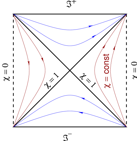
Figure 3: The Penrose-Carter diagram of deSitter space

When the bulk object is moving along the holographic screen $\mu=\mu_{B}$ itself, this is the fact used in [12] to obtain a microscopic interpretation of two dimensional deSitter entropy.

6 Higher dimensions

We have so far restricted our attention to $AdS_{3}$ for simplicity. The discussion, however, can be easily generalized to any $AdS_{d+1}$. The lesson we have learnt is that the boundary interpretation of Unruh radiation in the bulk lies in the appearance of cosmological spacetimes. From this point of view all we have to find is the relevant cosmology. This is easily done for any $d$ since we have also learnt that the class of observers who move with the hologram are specified by a coordinate system which is in fact an appropriate coordinate system in the bulk restricted to the boundary.

The transformation rules to these coordinates are in fact identical to those for $d=2$. This is because in our definitions of the various coordinate systems in terms of the globally embedding space of $(U,V,W_{i})$ (equations (105),(109) and (113)) we have used a common set of $(d-2)$ angles $\theta_{1}\cdots\theta_{d-2}$. Using this fact we can immediately write down the cosmology arising on the Poincaré boundary

$${\rm Subcritical}~{}~{}~{} ds^{2} ={1\over(\cos{\bar{\tau}}+\cos{\bar{\phi}})^{2}}[-d{\bar{\tau}}^{2}+d{\bar{\phi}}^{2}+\sin^{2}{\bar{\phi}}~{}d\Omega_{d-2}^{2}].$$

$${\rm Supercritical}~{}~{}~{} ds^{2} =e^{-2{\bar{\eta}}}[-d{\bar{\eta}}^{2}+d{\bar{\psi}}^{2}+\sinh^{2}{\bar{\psi}}~{}d\Omega_{d-2}^{2}].$$ (100)

For the Global boundary we have the spacetimes

$${\rm Critical}~{}~{}~{} ds^{2} ={4\over 4{\tilde{r}}^{2}+(1+{\tilde{t}}^{2}-{\tilde{r}}^{2})^{2}}[-d{\tilde{t}}^{2}+d{\tilde{r}}^{2}+{\tilde{r}}^{2}~{}d\Omega_{d-2}^{2}].$$

$${\rm Supercritical}~{}~{}~{} ds^{2} ={2\over\cosh 2{\bar{\eta}}+\cosh 2{\bar{\psi}}}[-d{\bar{\eta}}^{2}+d{\bar{\psi}}^{2}+\sinh^{2}{\bar{\psi}}~{}d\Omega_{d-2}^{2}].$$ (101)

Finally for the $d$ dimensional deSitter boundary in hyperspherical coordinates the following different metrics arise in the three different cases

$${\rm Subcritical}~{}~{}~{} ds^{2} ={1\over\sin^{2}{\tilde{\tau}}}[-d{\tilde{\tau}}^{2}+d{\tilde{\phi}}^{2}+\sin^{2}{\tilde{\phi}}~{}d\Omega_{d-2}^{2}].$$

$${\rm Critical}~{}~{}~{} ds^{2} ={1\over{\hat{t}}^{2}}[-d{\hat{t}}^{2}+d{\hat{r}}^{2}+{\hat{r}}^{2}~{}d\Omega_{d-2}^{2}].$$

$${\rm Supercritical}~{}~{}~{} ds^{2} =-\sin^{2}\theta d{\bar{\eta}}^{2}+d\theta^{2}+\cos^{2}\theta~{}d\Omega_{d-2}^{2}.$$ (102)

In particular for the supercritical case one has $d$ dimensional Milne universe on the Poincaré boundary and the stationary form of the $d$ dimensional deSitter metric on the hyperspherical boundary.

For $d\neq 2$ the one point functions can be also calculated using the results of [9]. However, the transformation properties of the one point function would not be as simple as for $d=2$.

7 Conclusions

The main lesson of our study is that there is a dual relationship between thermal behavior (or its absence) in cosmological spacetimes on the boundary and thermal behavior observed by uniformly accelerated objects in the bulk.

An interesting relationship between thermal effects due to acceleration and those due to “genunine” gravity effects has been uncovered in [6]. Here one considers some flat global embedding spacetime, typically with more than one timelike dimension, in which various nontrivial lower dimensional spacetimes, like deSitter , anti-deSitter or various kinds of black holes, are embedded by defining a suitable hypersurface. Accelerated trajectories in these lower dimensional spacetimes - e.g. those in $AdS$ spacetimes discussed in this paper, or those of stationary observers in a deSitter space or black hole background - then become uniformly accelerated trajectories in the higher dimensional flat emebdding spacetime. Thermal effects of the former, which may be thought of as “genuine” gravity effects, can be then obtained from Unruh effect in the embedding spacetime. Note that in this discussion the trajectories in the lower dimensional nontrivial spacetime are not holograms of those in the embedding space - they are the latter trajectories themselves. In other words the trajectories always lie in the lower dimensional space.

If we consider the $AdS$ space time of this paper as the global embedding spacetime, and the various boundaries are used to define lower dimensional spacetime, the situation may appear somewhat similar to the setup of [6]. However, the problem we have studied is rather different. In our work the trajectories in fact do not lie on the boundary. Rather they are transverse to the boundary and their holograms are expanding blobs on the boundary. The thermal behavior in the bulk now has an interpretation in terms of observers in appropriate cosmologies.

In one sense the problem addressed in [12] also appears similar to that in [6]. Here one considers the induced deSitter space on a constant $\mu$ surface in hyperspherical coordinates in $AdS_{3}$. Stationary observers in this deSitter space then become uniformly accelerated observers in the $AdS$ space with supercritical acceleration. However the crucial difference with [6] is that this constant $\mu$ surface, on which the bulk trajectory lies, is regarded as a holographic screen. Furthermore as opposed to the usual AdS/CFT setup (which is the one used in our work), $\mu$ is finite and dynamically determined in terms of the tension of a 1-brane which is on this surface. For the same reason, the holographic theory has dynamical gravity [14]. This allows a microscopic understanding of the thermodynamics measured by these stationary observers.

In our work we have argued that a similar correspondence between Unruh thermal properties of bulk objects moving transverse to the boundary and cosmological thermal properties on the boundary theory. The boundary is of course not the trajectory itself. Nevertheless, the presence or absence of thermal behavior follows from the appropriate choice of time in the boundary cosmology. This correspondence is in the traditional AdS/CFT framework and different choices of the boundary theory give rise to different cosmologies, which of course include deSitter spacetimes.

Finally we note that we have not obtained these conclusions from the boundary theory itself. Rather we have simply presented what the AdS/CFT predicts in the boundary theory. The outstanding task is to obtain these results starting from the specific CFT on the boundary. That would lead to a microscopic understanding. As usual, the problem is that one has to compute quantities at strong coupling. Nevertheless one may hope that some qualitative features can be nevertheless derived.

8 Acknowledgements

We would like to thank the High Energy Theory group and Cosmology and General Relativity group at YITP for providing a stimulating atmosphere and T. Yoneya for a discussion. A.Z. is also grateful to the Killam Trust for its support. S.R.D would like to thank the Theory group of University of Hokkaido for hospitality during the final stages of preparation of this manuscript.

9 Appendix I : Coordinate systems in $AdS_{d+1}$

All the three coordinate systems we have used in this paper are various ways of solving the basic definition of $AdS_{d+1}$ as a hyperboloid in $d+2$ dimensional flat space with two timelike coordinates. The coordinates in this embedding spacetime are denoted by $U,V,W_{i}$ with $i=1,\cdots D$. The metric in this emebdding space is

$$ds^{2}=-dU^{2}-dV^{2}+\sum_{i=1}^{d}dW_{i}^{2}$$ (103)

The $AdS_{d+1}$ is defined as the hyperboloid

$$-U^{2}-V^{2}+\sum_{i=1}^{d}W_{i}^{2}=-R^{2}$$ (104)

In the following we will measure all distances in units of $R$, so we will set $R=1$.

9.1 Global Coordinates

A global coordinate system on $AdS_{d+1}$ is defined as

$$U = \sec\nu~{}\cos\tau$$

$$V = \sec\nu~{}\sin\tau$$

$$W_{1} = \tan\nu~{}\cos\phi$$

$$W_{2} = \tan\nu~{}\sin\phi~{}\cos\theta_{1}$$

$$\cdots$$

$$W_{d} = \tan\nu~{}\sin\phi\sin\theta_{1}\cdots\sin\theta_{d-2}$$ (105)

The ranges of the coordinates are

$$0 < \nu<\pi/2$$

$$0 < \tau<2\pi$$

$$0 < \phi,\theta_{i}<\pi~{}~{}~{}~{}~{}~{}~{}~{}(i=2,\cdots(d-3))$$

$$0 < \theta_{d-2}<2\pi$$ (106)

These coordinates cover the entire $AdS_{d+1}$. It is sometimes conveninent to consider the covering space where $\tau$ ranges from $-\infty$ to $\infty$ by attaching identical copies. The metric follows from substituting (105) in (103)

$$ds^{2}=\sec^{2}\nu(-d\tau^{2}+d\nu^{2}+\sin^{2}\nu d\Omega_{d-1}^{2})$$ (107)

Surfaces of constant $\nu$ have spatial sections which are $S^{d-1}$. The global boundary is at $\nu=\nu_{B}\rightarrow\pi/2$ with the metric

$$ds_{gB}^{2}=-d\tau^{2}+d\Omega_{d-1}^{2}$$ (108)

9.2 Poincaré Coordinates

The Poincaré coordinate system is defined by the relationships

$$U = {1\over 2z}[1+(r^{2}+z^{2}-t^{2})]$$

$$V = {t\over z}$$

$$W_{1} = {1\over 2z}[1-(r^{2}+z^{2}-t^{2})]$$

$$W_{2} = {r\over z}\cos\theta_{1}$$

$$\cdots$$

$$W_{3} = {r\over z}\sin\theta_{1}\cos\theta_{2}$$

$$W_{d} = {r\over z}\sin\theta_{1}\sin\theta_{2}\cdots\sin\theta_{d-2}$$ (109)

where the ranges of the coordinates are

$$-\infty < t<\infty$$

$$0 < z<\infty$$

$$0 < r<\infty$$

$$0 < \theta_{i}<\pi~{}~{}~{}~{}~{}~{}~{}~{}(i=2,\cdots(d-3))$$

$$0 < \theta_{d-2}<2\pi$$ (110)

The metric is now

$$ds^{2}={1\over z^{2}}[-dt^{2}+dz^{2}+dr^{2}+r^{2}d\Omega^{2}_{d-2}]$$ (111)

The Poincaré system does not cover the entire $AdS$ spacetime. There is a horizon at $z=\infty$.

Surfaces of constant $z$ are $d$ dimensional flat spacetimes. The Poincaré boundary is at $z=z_{B}\rightarrow 0$ and has the standard flat metric upto an overall constant

$$ds_{PB}^{2}=-dt^{2}+dr^{2}+r^{2}d\Omega^{2}_{d-2}$$ (112)

9.3 “BTZ” Coordinates

The third coordinate system we will use will be referred to “BTZ”-type coordinates since this is a natural extension of the BTZ coordinates for $d=2$. These are defined by

$$U = {\sqrt{\rho^{2}-1}}\sinh\eta$$

$$V = \rho\cosh\psi$$

$$W_{1} = {\sqrt{\rho^{2}-1}}\cosh\eta$$

$$W_{2} = \rho\sinh\psi\cos\theta_{1}$$

$$\cdots$$

$$W_{3} = \rho\sinh\psi\sin\theta_{1}\cos\theta_{2}$$

$$W_{d} = \rho\sinh\psi\sin\theta_{1}\sin\theta_{2}\cdots\sin\theta_{d-2}$$ (113)

where the ranges of the coordinates are

$$-\infty < \eta<\infty$$

$$0 < \psi<\infty$$

$$1 < \rho<\infty$$

$$0 < \theta_{i}<\pi~{}~{}~{}~{}~{}~{}~{}~{}(i=2,\cdots(d-3))$$

$$0 < \theta_{d-2}<2\pi$$ (114)

The metric is now

$$ds^{2}=-(\rho^{2}-1)d\eta^{2}+{d\rho^{2}\over(\rho^{2}-1)}+\rho^{2}[d\psi^{2}+\sinh^{2}\psi d\Omega_{d-2}^{2}]$$ (115)

These coordinates also do not cover the entire $AdS$ spacetime and has horizons at $\rho^{2}=1$.

Surfaces of constant $\rho$ have spatial sections which are hyperbolic spaces in $(d-1)$ dimensions. The boundary is at $\rho=\rho_{B}\rightarrow\infty$ and has the metric

$$ds^{2}_{BTZB}=-d\eta^{2}+d\psi^{2}+\sinh^{2}\psi d\Omega_{d-2}^{2}$$ (116)

9.4 Hyperspherical Coordinates

These coordinates are analytic continuations of the standard polar coordinates on a $(d+1)$ dimensional sphere. In terms of the embedding space one has

$$U = \sinh\mu\sin\theta\sinh\eta$$

$$V = \cosh\mu$$

$$W_{1} = \sinh\mu\sin\theta\cosh\eta$$

$$W_{2} = \sinh\mu\cos\theta\cos\theta_{1}$$

$$\cdots$$

$$W_{3} = \sinh\mu\cos\theta\sin\theta_{1}\cos\theta_{2}$$

$$W_{d} = \sinh\mu\cos\theta\sin\theta_{1}\sin\theta_{2}\cdots\sin\theta_{d-2}$$ (117)

The time is the same as in BTZ coordinates and so are the angles $\theta_{i}$ with $i=1,\cdots(d-2)$. The ranges of the other two coordinates are

$$0 < \mu<\infty$$

$$1 < \theta<\pi$$

The metric is now

$$ds^{2}=-\sinh^{2}\mu\sin^{2}\theta d\eta^{2}+d\mu^{2}+\sinh^{2}\mu[~{}d\theta^{2}+\cos^{2}\theta~{}d\Omega_{d-2}^{2}~{}]$$ (119)

These coordinates do not cover the entire $AdS$ spacetime. Observers at a given point in space have a horizon at $\theta={\pi\over 2}$.

Surfaces of constant $\mu$ are $d$ dimensional deSitter spacetimes. The boundary is at $\mu=\mu_{B}\rightarrow\infty$ and has a stationary metric

$$ds^{2}_{HypB}=-\sin^{2}\theta d\eta^{2}+d\theta^{2}+\cos^{2}\theta~{}d\Omega_{d-2}^{2}$$ (120)

9.5 Coordinate transformations

The transformation rules between the various coordinates may be easily obtained by comparing their definitions in terms of the basic embedding coordinates $U,V,W_{i}$. Since we have chosen a common set of $(d-2)$ angles $\theta_{i}$ in all the three coordinate systems, this job is particularly simple : one has to just relate the sets $(\tau,\nu,\phi)$, $(t,z,r)$ ,$(\eta,\rho,\psi)$ and $(\eta,\mu,\theta)$. As a result these rules are same for all values of $d$. These formulae can be easily worked out from the above expressions.

10 Appendix II : Calculation of the field $\Phi(X)$

10.1 Subcritical Accelerations, $a^{2}<1$

First consider trajectories given by (28) which have accelerations $a^{2}<1$. Since these correspond to constant values of $\nu=\nu_{0}$ it is most conveninent to write down the Green’s function and the field $\Phi(X)$ in global coordinates. In (41) we thus have

$$Y(\lambda):\nu^{\prime}=\nu_{0}~{}~{}~{}\phi^{\prime}=0$$ (121)

The proper time interval $d\lambda$ along the trajectory is given by

$$d\lambda=\sec\nu_{0}d\tau^{\prime}=dv~{}\sec\nu_{0}~{}{d\tau^{\prime}\over dv}$$ (122)

Using (37) we get

$${d\tau^{\prime}\over dv}={\sin v\over[\sec^{2}\nu\sec^{2}\nu_{0}-(\cos v+\tan\nu\tan\nu_{0}\cos\phi)^{2}]^{1/2}}$$ (123)

Using (36) one gets

$$\Phi(X)={\sec\nu_{0}\over 2\pi}\int_{0}^{\pi}dv~{}{\cos v\over[\sec^{2}\nu\sec^{2}\nu_{0}-(\cos v+\tan\nu\tan\nu_{0}\cos\phi)^{2}]^{1/2}}$$ (124)

10.2 Critical Acceleration

For the trajectory (29) with critical acceleration one has

$$Y(\lambda):z^{\prime}=z_{0}~{}~{}~{}r=0$$ (125)

The proper time interval is given by

$$d\lambda={1\over z_{0}}dt^{\prime}=dv~{}{1\over z_{0}}~{}{dt^{\prime}\over dv}$$ (126)

and from (38) we obtain

$${dt^{\prime}\over dv}={zz_{0}\sin v\over[r^{2}+z^{2}+z_{0}^{2}-2zz_{0}\cos v]^{1/2}}$$ (127)

The field at a point $X=(t,r)$ then becomes

$$\Phi(X)={z\over 2\pi}\int_{0}^{\pi}dv~{}{\cos v\over[r^{2}+z^{2}+z_{0}^{2}-2zz_{0}\cos v]^{1/2}}$$ (128)

10.3 Supercritical Acceleration

A $a^{2}>1$ trajectory (30) is best described in BTZ coordinates as

$$Y(\lambda):\rho^{\prime}=\rho_{0}~{}~{}~{}~{}\psi=0$$ (129)

or equivalently in hyperspherical coordinates as

$$Y(\lambda):\mu=\mu_{0}~{}~{}~{}~{}~{}~{}\theta={\pi\over 2}$$ (130)

with

$$\rho_{0}=\cosh\mu_{0}$$ (131)

The proper time is now given by

$$d\lambda={\sqrt{\rho_{0}^{2}-1}}~{}d\eta^{\prime}={\sqrt{\rho_{0}^{2}-1}}~{}dv~{}{d\eta^{\prime}\over dv}$$ (132)

From the expression (39) one has

$${d\eta^{\prime}\over dv} = {\sin v\over[(\rho_{0}V-\cos v)^{2}+(\rho_{0}^{2}-1)(U^{2}-W_{1}^{2})]^{1/2}}$$ (133)

$$= {\sin v\over[(\rho\rho_{0}\cosh\psi-\cos v)^{2}-(\rho^{2}-1)(\rho_{0}^{2}-1)]^{1/2}}$$

Using the formula for the geodesic distance in BTZ coordinates we have

$$\Phi(X)={{\sqrt{\rho_{0}^{2}-1}}\over 2\pi}\int_{0}^{\pi}dv{\cos v\over[(\rho\rho_{0}\cosh\psi-\cos v)^{2}-(\rho^{2}-1)(\rho_{0}^{2}-1)]^{1/2}}$$ (134)

Similarly in hyperspherical coordinates we have

$$\Phi(X)={\sinh\mu_{0}\over 2\pi}\int_{0}^{\pi}dv{\cos v\over[\sinh^{2}\mu\sinh^{2}\mu_{0}\sin^{2}\theta-(\cosh\mu\cosh\mu_{0}-\cos v)^{2}]^{1/2}}$$ (135)

10.4 Transformation to appropriate coordinates

To extract the one point function for a particular boundary we need the expressions for $\Phi(X)$ in appropriate coordinates. As emphasized above, in the bulk $\Phi(X)$ is a scalar, so all we need to do is to rewrite the expressions above in these coordinates. This is easily done by using the definitions in Appendix I in terms of the embedding coordinates $(U,V,W_{i})$.

References

- [1] G. ’t Hooft, in “Salamfest” (1993) 0284, gr-qc/9310026; L. Susskind, J. Math. Phys. 36 (1995) 6377, hep-th/9409089.
- [2] J. Maldacena, Adv. Theo. Math. Phys. 2 (1998) 231, hep-th/9711200; S. Gubser, I. Klebanov and A. Polyakov, Phys. Lett. B428 (1998) 105, hep-th/ 9802109; E. Witten, Adv. Theo. Math. Phys. 2 (1998) 253, hep-th/9802150.
- [3] E. Witten, Adv. Theo. Math. Phys. 2 (1998) 505, hep-th/9803131.
- [4] A. Strominger and C. Vafa, Phys. Lett. B379 (1996) 99, hep-th/9601029; C. Callan and J. Maldacena Nucl. Phys. B472 (1996) 591, hep-th/9602043; A. Dhar, G. Mandal and S.R. Wadia, Phys. Lett. B388 (1996) 51, hep-th/9605234 ; S.R. Das and S.D. Mathur, Nucl. Phys. B478 (1996) 561, hep-th/9606185 ; J. Maldacena and A. Strominger, Phys. Rev. D55 (1997) 861, hep-th/9609026.
- [5] W. Unruh, Phys. Rev. D10 (1974) 3194; W. Unruh, Phys. Rev. D14 (1976) 870.
- [6] S. Deser and O. Levin, Class. Quant. Grav. 14 L 163; S. Deser and O. Levin, Class. Quant. Grav. 15 (1998) L85-L87,hep-th/9806223; S. Deser and O. Levin, Phys. Rev. D59 (1999) 064004, hep-th/9809159.
- [7] T. Jacobson, Class.Quant.Grav 15 (1998) 251, gr-qc/9709048.
- [8] V. Balasubramanian, P. Kraus and A. Lawrence, Phys. Rev. D59 (1999) 046003, hep-th/9805171; V. Balasubramanian, P. Kraus, A. Lawrence and S. Trivedi, Phys. Rev. D59 (1999) 104021, hep-th/9808017; T. Banks, G. Horowitz and E. Martinec, hep-th/9808; E. Keski-Vakkuri, Phys. Rev. D59 (1999) 104001, hep-th/9808037.
- [9] U. Danielsson, E. Keski-Vakkuri and M. Kruczenski, JHEP 9901 (1999) 002, hep-th/9812007.
- [10] See e.g. N.D. Birell and P.C.W. Davies, “Quantum fields in curved space”, Cambridge University Press, 1982, and references therein.
- [11] G.W. Gibbons and S.H. Hawking, Phys. Rev. D15 (1977) 2738.
- [12] S. Hawking, J. Maldacena and A. Strominger, hep-th/0002145.
- [13] S. Gubser, Phys. Rev. D63 (2001) 084017,hep-th/9912001 and J. DeBoer, E. Verlinde and H. Verlinde, JHEP 0008 (2000) 003,hep-th/9912012.
- [14] L. Randall and R. Sundrum, Phys. Rev. Lett. 83 (1999) 4690, hep-th/9906064
- [15] T. Fiola, J. Preskill, A. Strominger and S. Trivedi, Phys. Rev. D50 (1994) 3987, hep-th/9403137; T. Jacobson, gr-qc/9404039; V. Frolov, D. Furasev and A. Zelnikov, Nucl. Phys. B486 (1997) 339, hep-th/9607104; V. Frolov and D. Fursaev, Phys. Rev. D 56 (1997) 2212, hep-th/9703178.
- [16] U. Danielsson, A. Guijosa, M. Kruczenski and B. Sundborg, JHEP 0005 (2000) 028, hep-th/0004187; S.R. Das and B. Ghosh, JHEP 0006 (2000) 043, hep-th/0005007.
- [17] L. Susskind and E. Witten, hep-th/9805114.
- [18] T. Tanaka and M. Sasaki, Phys. Rev. D55 (1997) 6061.