Skyrmions on the Two-Sphere.

Abstract

We study static solutions of the Skyrme model on the two-sphere of radius $L$, for various choices of potential. The high-density Skyrmion phase corresponds to the ratio $\beta=L/{\rm(size\ of\ Skyrmion)}$ being small, whereas the low-density phase corresponds to $\beta$ being large. The transition between these two phases, and in particular the behaviour of a relevant order parameter, is examined.

1 Introduction

Topological solitons are usually studied on flat space, but there are several reasons why the curved-space setting is interesting (apart from the most obvious one of possible cosmological applications). First, it often reveals useful mathematical features; there are now two length scales, namely the size of the solitons and the radius of curvature of the underlying geometry, and there is an interplay between these scales. For monopole-like objects such as as vortices and Yang-Mills-Higgs monopoles, one can work on hyperbolic space: in the case of vortices, the equations for static vortices become integrable for a particular value of the curvature [1], [2]; and for YMH monopoles, the system is simpler on hyperbolic space than on flat space [3]. For textures, such as the Skyrmions discussed in this paper, one may study the problem on either hyperbolic spaces or spheres (ie on spaces of constant negative or positive curvature), and this similarly throws up interesting geometrical features [4], [5], [6], [7], [8], [9], [10].

There are also more physical reasons for studying textures on compact spaces, namely that this models a finite density of solitons, and the transistion between the high-density and the low-density phases. One may do this without introducing curvature, by taking space to be a flat torus; but it is in some ways simpler to use a sphere. This was first done for the Skyrme model in three spatial dimensions, which is a model of nuclear matter. But there has also been interest in the two-dimensional version, both as a ‘toy’ model and also because it has several potential applications in condensed-matter physics. In this paper, we study the Skyrme model on the two-sphere of radius $L$, and in particular the dependence on the ratio $\beta=L/{\rm(size\ of\ Skyrmion)}$.

In the three-dimensional Skyrme model (without a pion mass term), the Skyrmion for small $\beta$ is homogeneously spread out over space; when $\beta$ reaches a certain critical value, the Skyrmion localizes around a point [5], [10]. If the winding number is greater than one, or if a zeroth-order potential term (such as a mass term) is present, then this transistion is less clear-cut. In the two-dimensional case, such a potential term is obligatory, and so this smearing effect is inevitable (cf [8]). The quantity $\Phi$ which monitors the deviation from homogeneity tends to zero as $\beta$ does, but $\Phi$ is never quite zero, and so is not an order parameter in the strict sense. There is, however, another quantity $\Psi$ which does serve as an order parameter, namely one which monitors the breakdown of a certain reflection symmetry [6], [10]; and the associated phase transition is sharp (as long as the potential has this symmetry, which was not the case for the system studied in [8]). We shall investigate these phenomena, for several different potentials, by finding rotationally-symmetric solutions numerically.

2 Skyrme models on the two-sphere

In this section, we review the Skyrme system on the two-sphere, the topological Bogomol’nyi bound on its energy, and the imposition of rotational symmetry. Let $M$ denote the standard 2-sphere of radius $L$, with local coordinates $(x^{1},x^{2})$ and metric $ds^{2}=g_{jk}\,dx^{j}\,dx^{k}$. The area element on $M$ is $\omega=h\,dx^{1}\wedge dx^{2}$, where $h=[\det(g_{jk})]^{1/2}$. The Skyrme field $\phi$ is a map from $M$ to the unit sphere $S^{2}$, and may be thought of as a unit vector field $\vec{\phi}(x^{j})$ (so $\vec{\phi}\cdot\vec{\phi}=1$). We are considering only the static problem, so $\vec{\phi}$ depends only on the spatial variables $x^{j}$, and not on time. Let $\partial_{j}\vec{\phi}$ denote the partial derivative $\partial\vec{\phi}/\partial x^{j}$. The winding number (degree) of $\vec{\phi}$ is denoted by the integer $k$. If we define the function $\rho[\vec{\phi}]$ as the triple scalar product $\rho[\vec{\phi}]=2\vec{\phi}\cdot(\partial_{1}\vec{\phi})\times(\partial_{2}\vec{\phi})$, then (assuming that the $x^{j}$ cover almost all of $M$) we have

$$k=\frac{1}{8\pi}\int_{M}\rho[\vec{\phi}]\,dx^{1}\,dx^{2}.$$ (1)

The (normalized) energy $E_{k}$ of $\vec{\phi}$ is taken to be a sum of three terms $E_{k}=E^{(2)}+E^{(4)}+E^{(0)}$, with each being the integral over $S^{2}$ of the corresponding density function:

$$E^{(n)}=\frac{1}{4\pi|k|}\int_{M}{\cal E}^{(n)}[\vec{\phi}]\,\omega$$ (2)

for $n=2,4,0$. The densities ${\cal E}^{(n)}(\vec{\phi})$ are given by

$${\cal E}^{(2)}[\vec{\phi}] = \frac{1}{2}g^{jk}(\partial_{j}\vec{\phi})(\partial_{k}\vec{\phi}),$$ (3)

$${\cal E}^{(4)}[\vec{\phi}] = \frac{1}{8}\gamma h^{-2}\rho^{2},$$ (4)

$${\cal E}^{(0)}[\vec{\phi}] = \alpha V(\vec{\phi}),$$ (5)

where $\gamma$ and $\alpha$ are positive constants, and where $V(\vec{\phi})$ is some suitable function of $\vec{\phi}$ (not involving its derivatives). We regard the normalized energy as dimensionless. The constants $\gamma$ and $\alpha$ have dimensions of length² and length^-2 respectively; the dimensionless combination $\alpha\gamma$ determines the energy of a soliton, while its size is of order $(\gamma/\alpha)^{1/4}$. In flat space, this latter quantity simply sets the length scale; but on the sphere $M$, there already is a length scale $L$. So one has a dimensionless parameter $\beta=L(\alpha/\gamma)^{1/4}$, which is the ratio between the size of space and the size of the soliton. From now on, we shall set $\gamma=1$.

The energy of any configuration of nonzero degree satisfies a generalized Bogomol’nyi bound [11]. First, $E^{(2)}$ satisfies the standard O(3) sigma-model bound $E^{(2)}\geq 1$. To get a bound on $E^{(4)}+E^{(0)}$, write ${\cal E}^{(0)}=G^{2}/2$ and observe that

$$E^{(4)}+E^{(0)} = \frac{1}{8\pi|k|}\int_{M}\bigl{[}(h^{-1}\rho/2-G)^{2}+h^{-1}\rho\,G\bigr{]}\,\omega$$

$$\geq \frac{1}{8\pi|k|}\int_{M}\rho\,G\,dx^{1}\,dx^{2}$$

$$= \frac{1}{4\pi}\int_{S^{2}}G(\vec{\phi})\,\,\vec{\phi}\cdot d\vec{\phi}\times d\vec{\phi}\,;$$

the last equality follows from the degree theorem $\int\phi^{*}(G\Omega)=k\int G\Omega$, with $\Omega=\vec{\phi}\cdot d\vec{\phi}\times d\vec{\phi}$ being the area element on the target sphere $S^{2}$. If $G$ depends only on the third component $\phi^{3}$ of $\vec{\phi}$, which is the case for all the examples that we consider, then the bound on the total energy takes the form

$$E_{k} \geq 1+\frac{1}{2}\int_{-1}^{1}G(\phi^{3})\,d\phi^{3}$$ (6)

$$= 1+\sqrt{\alpha/2}\int_{-1}^{1}\sqrt{V(\phi^{3})}\,d\phi^{3}.$$

In this paper, we study rotationally-symmetric configurations. Let us use polar coordinates $(\theta,\varphi)$ on $M$, so that $ds^{2}=L^{2}(d\theta^{2}+\sin^{2}\theta\,d\varphi^{2})$ and $h=L^{2}\sin\theta$. We impose rotational symmetry by taking $\vec{\phi}$ to have the form

$$\vec{\phi}=\bigl{(}\sin(f)\cos(k\varphi),\sin(f)\sin(k\varphi),\cos(f)\bigr{)},$$ (7)

where $k$ is an integer and $f=f(\theta)$. Assuming that this profile function $f(\theta)$ satisfies the boundary conditions $f(0)=\pi$ and $f(\pi)=0$, the configuration (7) has winding number $k$. Its normalized energy is

$$E_{k}=\frac{1}{4|k|}\int_{0}^{\pi}\biggl{[}(f^{\prime})^{2}+k^{2}\biggl{(}\frac{\sin f}{\sin\theta}\biggr{)}^{2}+\biggl{(}\frac{kf^{\prime}}{L}\frac{\sin f}{\sin\theta}\biggr{)}^{2}+2L^{2}{\cal E}^{(0)}(\cos f)\biggr{]}\sin\theta\,d\theta,$$ (8)

where $f^{\prime}=df/d\theta$ and where we are (as mentioned above) taking ${\cal E}^{(0)}$ to be a function of $\phi^{3}=\cos f$ only.

We are interested in the stationary points of the functional (8), and we find these numerically (with an accuracy better than $0.1\%$). Two independent methods were used: first, a direct minimization of (8) by a conjugate-gradient method; and secondly, solving the corresponding Euler-Lagrange equations.

One particular ‘trial’ profile which is of interest is the one corresponding to a rotationally-symmetric conformal map (cf [5], [8], [10]). Such a profile can be used for any value of $k$, but we shall restrict here to the case $k=1$. The profile function $f(\theta)$ is then given by

$$\cot(f/2)=\lambda\tan(\theta/2),$$ (9)

where $\lambda$ is a positive constant. Notice that if $\lambda=1$, then $f(\theta)=\pi-\theta$, and this corresponds to the identity map from $M\cong S^{2}$ to $S^{2}$. This identity map is only a solution of the equations of motion if ${\cal E}^{(0)}$ is constant (ie not depending on $\vec{\phi}$). Another way of putting this is that if (and only if) ${\cal E}^{(0)}$ is constant, then Skyrmions spread out to fill the whole of space homogeneously, in the sense that the energy density ${\cal E}$ is constant. The configuration (9) has $E^{(2)}(\lambda)=1$ and $E^{(4)}(\lambda)=(\lambda^{4}+\lambda^{2}+1)/(6L^{2}\lambda^{2})$. Notice that $E^{(4)}(\lambda)$ has its minimum at $\lambda=1$; but the location (and existence) of a minimum in the total energy $E(\lambda)$ depends on the choice of the potential term $E^{(0)}$. The question is: for a given $L$ and choice of $E^{(0)}$, what are the minima of $E(\lambda)$, and in particular are they at $\lambda=1$ or at $\lambda\neq 1$?

We now wish to define the two quantities $\Phi$ and $\Psi$ mentioned in the introduction. The first of these is

$$\Phi=\langle(\phi^{3})^{2}\rangle-\frac{1}{3}=\frac{1}{4\pi L^{2}}\int_{M}(\phi^{3})^{2}\,\omega\,-\frac{1}{3}\,.$$ (10)

This is zero for the homogeneous configuration $f(\theta)=\pi-\theta$, and so gives an indication of the deviation from homogeneity. The second quantity is

$$\Psi=\langle\phi^{3}\rangle^{2}=\biggl{[}\frac{1}{4\pi L^{2}}\int_{M}\phi^{3}\,\omega\biggr{]}^{2}\,.$$ (11)

This is zero for configurations which have the reflection symmetry $\phi^{3}\mapsto-\phi^{3}$, but nonzero if the Skyrmion is localized around the point $\theta=0$ or $\theta=\pi$.

3 Two asymmetric examples

In this section, we give a brief discussion of two systems, arising from two possible choices of ${\cal E}^{(0)}$. Each is ‘asymmetric’, in the sense that neither posesses the symmetry $\phi^{3}\mapsto-\phi^{3}$. So a Skyrmion in these systems will never have $\Psi=0$; the field prefers to be near $\vec{\phi}=(0,0,1)$ rather than $\vec{\phi}=(0,0,-1)$. The first example (for corresponding flat-space studies see [12], [13]) is motivated by the question: can one saturate the Bogomol’nyi bound (6)? We shall not give a complete analysis of this question here; but in the $k=1$ case, it is easy to derive the following fact: the configuration (9) saturates the Bogomol’nyi bound if and only if ${\cal E}^{(0)}$ is given by

$${\cal E}^{(0)}=\frac{1}{2}\biggl{[}\frac{(\lambda^{2}+1)-(\lambda^{2}-1)\phi^{3}}{2L\lambda}\biggr{]}^{4}.$$ (12)

(Notice that the $\lambda=1$ case is degenerate: ${\cal E}^{(0)}$ is then constant.) For this system, the bound is

$$E\geq 1+(\lambda^{4}+\lambda^{2}+1)/(3L^{2}\lambda^{2}).$$ (13)

If, for example, we choose $\lambda=2L$, then the configuration (9) is a solution with energy

$$E=\frac{28L^{4}+4L^{2}+1}{12L^{4}}=\frac{7}{3}+O(L^{-2});$$ (14)

in the limit $L\to\infty$, this corresponds to [12], [13] with their parameters $\theta_{1}$ and $\theta_{2}$ set equal to $0.5$ and $1$ respectively (note also that their expression for energy $E$ is $2\pi$ times ours). The energy (14) is a monotonic-decreasing function of $L$; this remains true for variations of (12) such as ${\cal E}^{(0)}=(1-\phi^{3})^{4}$, and for $k>1$.

In this system, there is a repulsive force between solitons [12], [13], [14]. Consequently, one expects that the minimum-energy configurations for $k>1$ will not be rotationally-symmetric (or, equivalently, that all rotationally-symmetric $k>1$ configurations are unstable). So investigation of the $k>1$ sectors requires a full two-dimensional study.

The comments of the previous paragraph apply equally well to our other example in this section, which was the one studied in [15], [16], [17] (on flat space) and [8] (on the sphere). For this system, we have $V(\phi^{3})=1-\phi^{3}$. The Bogomol’nyi bound (6) becomes $E_{k}\geq 1+4\sqrt{\alpha}/3$ (note that this is stronger than the bound given in [8]). Here we give a brief description of the $k=1$ case, taking $\alpha=0.1$. For the $\lambda$-approximation (9), we have

$$E^{(0)}(\lambda)=\frac{2L^{2}\alpha}{1-\lambda^{2}}\biggl{[}1+\frac{\lambda^{2}\log(\lambda^{2})}{1-\lambda^{2}}\biggr{]},$$ (15)

which is a decreasing function of $\lambda$. The total energy $E(\lambda)$ has a minimum at $\lambda=\lambda_{{\rm min}}$, with $\lambda_{{\rm min}}>1$ depending on the parameter $\beta=L\alpha^{1/4}$. In figure 1, we plot the energy $E(\lambda_{{\rm min}})$, the actual Skyrmion energy $E=E_{1}$ (the minimum of (8)), and the quantities

(a) Energies $E$ and $E(\lambda_{{\rm min}})$

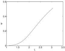
(b) $\Psi$

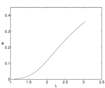
(c) $\Phi$

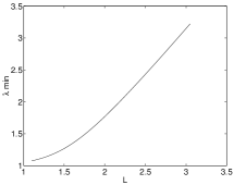
(d) $\lambda_{{\rm min}}$

Figure 1: Properties of a single Skyrmion, for the system with $V=1-\phi^{3}$, as a function of $L$. In (a), the dot-dashed line is the Bogomol’nyi bound, the solid curve is the actual energy, and the dashed curve is the best $\lambda$-approximation.

$\Psi$, $\Phi$ and $\lambda_{{\rm min}}$, all as functions of $L$. Notice that the lowest value of $E$ (when $L=1.65$ and $\beta=0.93$) is $1.424$, which less than $0.2\%$ greater than the Bogomol’nyi bound $1.4216$. At this value of $L$, we have $\lambda_{{\rm min}}=1.39$ and $E(\lambda_{{\rm min}})=1.425$. As $L\to\infty$, the energy of the Skyrmion tends to its flat-space value of $1.549$ [18].

As was noted in [8], there is a regime ($\beta<1$) where the Skyrmion is approximately spread out over $M$ and well-approximated by the configuration (9), and one ($\beta>1$) where the Skyrmion is localized and not well-approximated by (9). But the transition between these two regimes is not sharply-defined, and is not a phase transistion in the usual sense. This is partly due to the asymmetry of the system. In our next examples, we shall see a sharper transition.

4 Two symmetric examples

In this section, we study the systems which are defined, respectively, by $V(\phi^{3})=1-(\phi^{3})^{2}$ and $V(\phi^{3})=(\phi^{3})^{2}[1-(\phi^{3})^{2}]$. In these systems, Skyrmions attract one another [18], [14]; and consequently the solutions with $k>1$ have rotational symmetry. Since these potentials have the symmetry $\phi^{3}\mapsto-\phi^{3}$, one expects (in the rotationally-symmetric case, and for large $L$) that there will be a stable Skyrmion solution localized at a point (either $\theta=0$ or $\theta=\pi$); and also that there exists a solution which is symmetric under $\theta\mapsto\pi-\theta$ (and which may or may not be stable). For small $L$, however, only the symmetric solution exists.

First take $V(\phi^{3})=1-(\phi^{3})^{2}$, with the value $\alpha=0.08873$ (this corresponds to the value used in the flat-space study of [18], and allows a quantitative comparison with its results). The Bogomol’nyi bound (6) is $E\geq 1+\pi\sqrt{\alpha/8}=1.3309$. Let us look first at the $k=1$ sector. For the $\lambda$-approximation (9), we have

$$E^{(0)}(\lambda)=\frac{4\alpha L^{2}\lambda^{2}}{(1-\lambda^{2})^{2}}\biggl{[}-2-\frac{1+\lambda^{2}}{1-\lambda^{2}}\log(\lambda^{2})\biggr{]},$$ (16)

which is a positive function with a maximum at $\lambda=1$ (recall that $E^{(4)}(\lambda)$ has a minimum at $\lambda=1$). Notice that $E(\lambda^{-1})=E(\lambda)$; this corresponds to the $\phi^{3}\mapsto-\phi^{3}$ symmetry of $E[\vec{\phi}]$ in this case. So $\lambda=1$ gives either a minimum or a local maximum of $E(\lambda)$, depending on the value of $L$. A simple calculation reveals that if $\beta^{4}\leq 5/2$, then

$$E(1)=1+\frac{1}{2L^{2}}+\frac{2L^{2}\alpha}{3}$$ (17)

is a minimum of $E(\lambda)$; while if $\beta^{4}>5/2$, then there is a local maximum at $\lambda=1$, and the minima are at $\lambda_{{\rm min}}>1$ and $1/\lambda_{{\rm min}}$. Consequently, if we restrict to the special profiles (9), then there is a sharp phase transition at $\beta^{4}=5/2$ between a homogeneous phase ($\lambda=1$) and one where the Skyrmion localizes at a point (in this case, one of the poles) of the sphere $M$. Notice also that the lowest value of $E(1)$, namely $E=1+\sqrt{4\alpha/3}=1.344$, is attained when $\beta^{4}=3/4\Leftrightarrow L=1.705$.

This is just an approximation; the true Skyrmion energy is strictly less than $E(\lambda)$. However, there is indeed a minimum at $L=1.705$ (with $E=1.341$, only $0.2\%$ less than the $\lambda$-approximation); and there is a transition at $\beta^{4}=5/2\Leftrightarrow L=2.304$, as one can see from figure 2.

(a) Energies for $k=1$

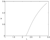
(b) $\Psi$

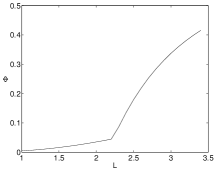
(c) $\Phi$

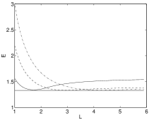
(d) Energies for $k=1,2,3$

Figure 2: Skyrmion properties for the system with $V=1-(\phi_{3})^{2}$, as a function of $L$. In (a), the dot-dashed line is the Bogomol’nyi bound; the solid curve is the energy of the symmetric solution; and the dashed curve is the energy of the asymmetric solution. Figures (b) and (c) plot the quantities $\Psi$ and $\Phi$ for the $k=1$ minimum. Figure (d) gives minimum energies for $k=1$ (solid curve), $k=2$ (dashed curve) and $k=3$ (dot-dashed curve); the solid line is the Bogomol’nyi bound.

Figure 2(a) depicts the energies of two static $k=1$ solutions, as functions of $L$. The solid curve is the energy of the ‘symmetric’ solution, ie the one satisfying $f(\pi-\theta)=\pi-f(\theta)$. This is obtained by starting with the configuration $f(\theta)=\pi-\theta$ and iterating towards a stationary point; our procedures are able to converge to a saddle-point (which this is for large $L$). The dashed curve is the energy of an asymmetric solution, obtained by starting with a highly-asymmetric configuration. We see that for $\beta^{4}<5/2$, the two solutions coincide; but for $\beta^{4}>5/2$, the former becomes unstable (numerical experiment indicates that it is a saddle-point rather than a local minimum). The corresponding parameters $\Psi$ and $\Phi$ for the minimum-energy solution are plotted in figures 2(b) and 2(c); note that when $\beta^{4}<5/2$, we have $\Psi=0$ (the solution is symmetric), but $\Phi\neq 0$ (it is not homogeneous). There is a second-order phase transition at $\beta^{4}=5/2$. In figure 2(d), the Skyrmion energies (minima of $E$) are plotted for $k=1,2,3$. It might be noted that $E_{k}$ gets very close to the Bogomol’nyi bound, at $L=1.7$, $L=2.9$ and $L=4.3$ for $k=1,2,3$ respectively (only $0.1\%$ above for $k=2$). As $L\to\infty$, we have [18]

$$E_{1}\to 1.564,\quad E_{2}\to 1.405,\quad E_{3}\to 1.371.$$ (18)

Now let us turn to the system with $V(\phi^{3})=(\phi^{3})^{2}[1-(\phi^{3})^{2}]$, taking $\alpha=0.04$ (which is consistent with the choice made in [14]). The Bogomol’nyi bound is $E\geq 1+\sqrt{2\alpha}/3=1.0943$. In the $k=1$ sector, the $\lambda$-approximation (9) has

$$E^{(0)}(\lambda)=\frac{4L^{2}\alpha\lambda^{2}\bigl{[}(10+18\lambda^{2}-18\lambda^{4}-10\lambda^{6})+(3+21\lambda^{2}+21\lambda^{4}+3\lambda^{6})\log(\lambda^{2})\bigr{]}}{3(\lambda^{2}-1)^{5}},$$ (19)

which has a local minimum at $\lambda=1$, with $E^{(0)}(1)=2L^{2}\alpha/15$. Consequently, $E(\lambda)$ always has a local minimum at $\lambda=1$. Notice that for $L=[15/(4\alpha)]^{1/4}=3.11$ (where the true energy has its lowest value $1.1026$), the approximation has energy $E(1)=1+\sqrt{4\alpha/15}=1.1033$.

There are two values $L_{1}$ and $L_{2}$ which are critical in the following sense. For $L\leq L_{1}$, $E(\lambda)$ has only one stationary point (the minimum at $\lambda=1$). For $L>L_{1}$, $E(\lambda)$ has three local minima: a symmetric one ($\lambda=1$) and a degenerate asymmetric one ($\lambda\neq 1$). For $L_{1}<L<L_{2}$, the asymmetric minimum has higher energy than the symmetric one: see figure 3(a), where $E$ is plotted as a function of $\mu=(\lambda^{2}-1)/(\lambda^{2}+1)$, for $L=7.4$. Finally, for $L>L_{2}$, the asymmetric minimum has the lower energy (cf. figure 3(b), for $L=8.4$); and the energy of the symmetric minimum tends to infinity as $L\to\infty$.

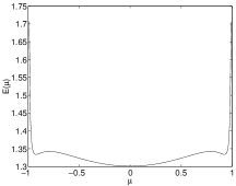
(a) Energy $E(\mu)$ for $L=7.4$

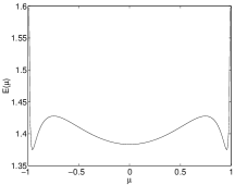
(b) Energy $E(\mu)$ for $L=8.4$

Figure 3: Energy $E(\mu)$ of the approximation (9), for the system with $V=(\phi_{3})^{2}[1-(\phi_{3})^{2}]$, where $\lambda^{2}=(1+\mu)/(1-\mu)$. For $L=7.4$, the symmetric ($\mu=0$, $\lambda=1$) minimum has lower energy than the asymmetric minima. For $L=8.4$, the asymmetric minima are lower.

This approximate picture suggests that for $L$ large enough, there are two stable Skyrmion solutions (symmetric and asymmetric); but that only the latter survives in the limit as $L\to\infty$. Our numerical investigation shows that this is indeed the case. Results from minimizing (8) are presented in figure 4.

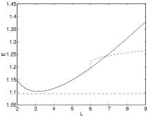
(a) Energies for $k=1$

(b) $\Psi$

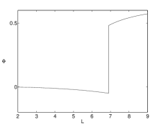
(c) $\Phi$

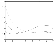
(d) Energies for $k=1,2,3$

Figure 4: Skyrmion properties for the system with $V=(\phi_{3})^{2}[1-(\phi_{3})^{2}]$, as a function of $L$. In (a), the dot-dashed line is the Bogomol’nyi bound; the solid curve is the energy of the symmetric solution; and the dashed curve is the energy of the asymmetric solution. Figures (b) and (c) plot the quantities $\Psi$ and $\Phi$ for the minimal-energy $k=1$ solution. Figure (d) gives the energy for $k=1$ (solid curve), $k=2$ (dashed curve) and $k=3$ (dot-dashed curve), for the minimal-energy solutions.

In figure 4(a), the solid curve is the energy of the symmetric $k=1$ solution; while the dashed curve is the energy of the asymmetric solution, which exists only for $L\geq L_{1}\approx 6$. For $L_{1}<L<L_{2}\approx 6.9$, the energy of the asymmetric solution is greater than that of the symmetric solution. Numerical evidence indicates that each of these solutions is stable (ie is a local minimum of the energy), at least in the rotationally-symmetric class. The stability of the symmetric solution, even for large $L$, is a consequence of the form of the potential $V=(\phi^{3})^{2}[1-(\phi^{3})^{2}]$, which favours $\phi^{3}=0\Leftrightarrow f(\theta)=\pi/2$. It also favours $\phi^{3}=\pm 1$, which stablizes the asymmetric solution. Between these local minima there will be a saddle-point solution, but we have not investigated this.

Figures 4(b) and 4(c) show the quantities $\Psi$ and $\Phi$ for the minimal-energy $k=1$ solution; and in figure 4(d), the minimal energy is plotted for $k=1,2,3$. As $L\to\infty$, we have [14]

$$E_{1}\to 1.281,\quad E_{2}\to 1.166,\quad E_{3}\to 1.143.$$ (20)

5 Concluding Remarks

We have studied rotationally-symmetric static solutions of the Skyrme model on the two-sphere of radius $L$. Even in the sector with winding number $k$ equal to unity, the properties of the solutions, and of the transition between the high-density (small $L$) and low-density (large $L$) phases, depends crucially on the choice of potential term.

It should be instructive to investigate the $k>1$ solution spaces in more detail (cf [10], [14], [18]). For symmetric potentials (such as those of section 4), this can be done within the rotationally-symmetric class; this is the analogue of the rational-map ansatz [10] in three dimensions. But for asymmetric potentials such as those of section 3, one expects a different picture: the Skyrmions should separate and form some pattern on $S^{2}$ as their optimal configuration. Flat-space studies [14] indicate that this pattern will, in general, be rather complicated.

References

- [1] E Witten, Some exact multi-instanton solutions of classical Yang-Mills theory. Phys Rev Lett 38 (1977) 121–124.
- [2] I A B Strachan, Low-velocity scattering of vortices in a modified Abelian Higgs model. J Math Phys 33 (1992) 102–110.
- [3] M F Atiyah, Magnetic monopoles in hyperbolic space. In: Proc Bombay Colloquium on Vector Bundles (Tata Institute and Oxford University Press, 1984), pp 185–187.
- [4] N S Manton and P J Ruback, Skyrmions in flat space and curved space. Phys Lett B 181 (1986) 137–140.
- [5] N S Manton, Geometry of Skyrmions. Commun Math Phys 111 (1987) 469–478.
- [6] A D Jackson, N S Manton and A Wirzba, New skyrmions solutions on a 3-sphere. Nucl Phys A 495 (1989) 499–522.
- [7] N S Manton and P J Ruback, Skyrmions on and from instantons. J Phys A 23 (1990) 3749–3759.
- [8] N N Scoccola and D R Bes, Two-dimensional skyrmions on the sphrere. JHEP 09 (1998) 012.
- [9] S-T Hong, The static properties of hypersphere skyrmions. Phys Lett B 417 (1998) 211–216.
- [10] S Krusch, Skyrmions and the rational map ansatz. Nonlinearity 13 (2000) 2163–2185.
- [11] J M Izquierdo, M S Rashid, B Piette and W J Zakrzewski, Models with solitons in (2+1) dimensions. Z Phys C 53 (1992) 177–182.
- [12] R A Leese, M Peyrard and W J Zakrzewski, Soliton scatterings in some relativistic models in (2+1) dimensions. Nonlinearity 3 (1990) 773–807.
- [13] P M Sutcliffe, The interaction of Skyrme-like lumps in (2+1) dimensions. Nonlinearity 4 (1991) 1109–1121.
- [14] P Eslami, M Sarbishaei and W J Zakrzewski, Baby skyrme models for a class of potentials. it Nonlinearity 13 (2000) 1867–1881.
- [15] B M A G Piette, H J W Müller-Kirsten, D H Tchrakian and W J Zakrzewski, A modified Mottola-Wipf model with sphaleron and instanton fields. Phys Lett B 320 (1994) 294–298.
- [16] B M A G Piette, B J Schroers and W J Zakrzewski, Multisolitons in a two-dimensional Skyrme model. Z für Physik C 65 (1995) 165–174.
- [17] B M A G Piette, B J Schroers and W J Zakrzewski, Dynamics of baby Skyrmions. Nucl Phys B 439 (1995) 205–235.
- [18] T Weidig, The baby skyrme models and their multi-skyrmions. Nonlinearity 12 (1999) 1489–1503.