hep-th/0103045

UA/NPPS-03-2001

New Perspectives on Moving Domain Walls in $(A)dS_{5}$ Space

Georgios Kofinas

University of Athens
Physics Department
Nuclear and Particle Physics Section
Panepistimioupolis, Ilisia GR 157 71
Athens, Greece

A new moving domain wall solution is obtained for a flat 3-universe. This consists of a bulk metric depending on both time and the extra coordinate, plus a dynamically interacting domain wall, admitted by the metric and inhabited by the three-universe. The matter contents are cosmological constants on the domain wall and the bulk. The bulk space is shown to be $(A)dS_{5}$. A remarkable fact concerning the three-universe is that its scale factor never vanishes, even though the corresponding scale factor of the bulk metric vanishes. The inclusion of a bulk scalar field is discussed, neglecting back-reaction. Its normalizability and the existence of a positive frequency or adiabatic bulk vacuum are shown.









March, 2001

1    Introduction

Over the last few years a lot of interest has been raised on the possibility that our universe is a three-brane embedded in a higher dimensional spacetime (bulk). Ordinary matter fields are assumed to live on the brane while gravity propagates in the whole spacetime. The major part of the work done in this direction refers to branes sitting at a prescribed point of an extra dimension. However, it is tempting, even inspired by $Dp$-brane models, to consider that the 3-brane is somehow let to move in the big spacetime. One such idea was introduced in [1], where the universe three-brane follows the classical geodesics of a spherical background bulk geometry and its dynamics is governed by the DBI action. A different idea, where gravitational back-reaction effects are included in the motion of the brane, i.e. the brane interacts with the whole bulk metric which is not however prescribed, was analysed in [2, 3].

In the present paper, we will adopt the term “moving domain wall” for a ($D-2$)-dimensional spacelike surface moving in a $D$-dimensional bulk space. More explicitly, a “domain wall that moves” will be a $D-2$ object (we even use the term “moving three-universe” when we discuss the case $D=5$). The term “domain wall” will be used for a ($D-1$)-dimensional hypersurface. When a domain wall moves in the big space, it forms a thin shell (hypersurface). If Einstein’s gravity resides in the bulk space, the matter source carried by the moving domain wall makes the stress-energy tensor of the domain wall a distributional source for the Einstein equations. In such a case of a thin shell it was proved long ago [4] that the discontinuity of the extrinsic curvature $K_{AB}$ of the shell is related to the energy-momentum tensor $T_{AB}$ of the matter on the shell by the “Israel matching conditions”

$$[K_{AB}-K_{C}^{C}h_{AB}]=-\kappa_{(D)}^{2}T_{AB},$$ (1)

where $h_{AB}$ is the induced metric on the shell and $\kappa_{(D)}^{2}=8\pi G_{(D)}$. In [2, 3] the bulk on both sides of the wall was assumed to be static and then consistency of the Israel conditions yielded non-trivial relationships between the metric in the bulk and the matter on the wall. These were proved to be compatible with the Einstein equations in the bulk, and thus, static spacetime solutions were obtained. Some of these solutions possess black hole or cosmological horizons, beyond which the domain wall moves in purely time-dependent bulks. In the present work, we follow this general idea but we abandon the static ansatz for the $D-2$ metric, allowing for the scale factor of the metric to be a function of both time and the extra coordinate. The matter content of our model consists of cosmological constants on both the (moving) domain wall and the bulk, instead of fields. The solution found is a special solution for the flat three-universe, but is the general solution for the zero value of some parameter $\mathcal{C}$ encountered. In [5] the domain wall moves obeying the Israel conditions in a fixed black hole background. In [6] a moving domain wall solution was obtained for a different ansatz for the bulk metric. Our analysis is performed for $D$ dimensions in the big space, though our primary interest lies in $D=5$, where in this case, the moving domain wall is supposed to represent our three-universe. A remarkable feature of our solution is that the scale factor of the three-universe never vanishes, i.e. the universe manages to avoid collapsing, while the bulk geometry has an apparent singularity.

One of the attractive features of higher dimensional models is that they provide new ways to solve the hierarchy problem. It has been shown [7] that if the higher dimensional spacetime is approximately a product of a 4-dimensional spacetime with a “large” compact space, then the higher dimensional scale of gravity, identified with the string scale, can be several orders of magnitude lower than the effective four-dimensional Planck scale. In a second scenario [8], it was shown that, for a particular four-metric depending on the bulk coordinate (non factorizable), the Planck scale is determined by the higher dimensional curvature, rather than the size of the extra dimension, which may be infinite. It was also shown there, that there is a single gravitational bound state confined to the brane, which corresponds to the graviton. In our case, instead of an analysis of some tensor perturbations of the metric, a study of an additional bulk scalar field on the found background geometry (neglecting back-reaction) has been performed. This field is seen to be normalizable with respect to the extra coordinate, while its time-dependent part allows a consistent definition of a bulk vacuum.

The structure of the paper is as follows: In section 2, we derive the dynamical equations of motion of a domain wall in a broad class of bulk metrics, generalizing in this way the result of [2]. Then, adopting an ansatz for the metric and for the matter contents chosen, we arrive at some differential relation between the bulk metric and the wall matter. In section 3, specializing to a flat three-universe, we show that the above relation is compatible with the bulk Einstein equations and the complete bulk solution is obtained. In section 4, the three-universe trajectory, as well as its own time evolution is discussed, for the various parameters of the model. In section 5, a scalar field is considered on the found bulk background, without back-reacting on it, and the wave equation is solved. Then, normalizability of the field is discussed and a positive frequency or adiabatic vacuum in the bulk space is shown to exist. Finally, in section 6, we conclude and speculate on possible generalizations.

2    Dynamic Domain Wall Motion

The purpose of this section is to derive the equations of motion of a domain wall moving in the bulk cosmological metric of a block-diagonal form

$$ds^{2}=g_{AB}dx^{A}dx^{B}=\varepsilon N^{2}(t,y)dt^{2}+b^{2}(t,y)dy^{2}+g_{ij}(t,y,x)dx^{i}dx^{j},$$ (2)

where the positive definite metric $g_{ij}$ defines the line element of the ($D-2$)- dimensional space. In this section we keep for completeness the full matrix $g_{ij}$ instead of only one scale factor for the $D-2$ part. We also keep the symbol $\varepsilon=\pm 1$ for future treatment of instanton solutions. Throughout this article, we will adopt the following convention for indices: capital Latin letters $A,B,...=1,...,D$ will denote full spacetime, while lower Latin $i,j,...=1,...,D-2$ are spacelike indices parallel to the moving domain wall.

Let the position of the moving domain wall in the bulk space be determined by a function $y(t)$, which we seek to find. The unit normal to the hypersurface formed by this motion (pointing for $Nb>0$ to the region with $y<y(t)$) is

$$n^{A}=\frac{Nb}{\sqrt{N^{2}+\varepsilon b^{2}\dot{y}^{2}}}\,\Big{(}\frac{\varepsilon}{N^{2}}\,\dot{y},\,-\frac{1}{b^{2}},\,\vec{0}\,\Big{)},$$ (3)

where $\dot{y}=\frac{dy}{dt}$. If $\tau$ is the proper time measured by the moving domain wall, then $\{\tau,x^{i}\}$ is a coordinate patch on the hypersurface and the induced metric on this is written as

$$ds_{(D-1)}^{2}=\varepsilon d\tau^{2}+g_{ij}^{(DW)}(\tau)dx^{i}dx^{j}.$$ (4)

The moving domain wall proper velocity vector field is $\mathrm{e}=\frac{d}{d\tau}$. Obviously, $\mathrm{e}^{A}\mathrm{e}_{A}=\varepsilon$, $\mathrm{e}^{A}n_{A}=0$. The domain wall can be given in parametrized form by equations $t=t(\tau)$, $y=y(\tau)$. If $t(\tau)$ is to be an increasing function, then $\mathrm{e}^{A}$ gets the form

$$\mathrm{e}^{A}=\frac{1}{\sqrt{N^{2}+\varepsilon b^{2}\dot{y}^{2}}}\,(1,\,\dot{y},\,\vec{0}\,).$$ (5)

The relation between $t$ and $\tau$ is

$$\frac{dt}{d\tau}=\frac{1}{\sqrt{N^{2}+\varepsilon b^{2}\dot{y}^{2}}}\,.$$ (6)

Obviously, the moving domain wall proper time is different than the proper time of the bulk space.

We shall now compute the extrinsic curvature $K_{AB}=h_{A}^{C}h_{B}^{D}\nabla_{C}n_{D}$ of the hypersurface, where $h_{AB}=g_{AB}-n_{A}n_{B}$. It is easier to do this in the non-holonomic basis $\{\mathrm{e},n,\partial_{i}\}$. The spatial components are

$$K_{ij}=\frac{1}{2\sqrt{N^{2}+\varepsilon b^{2}\dot{y}^{2}}}\left(\frac{\varepsilon b}{N}\,\dot{y}\,\partial_{t}g_{ij}-\frac{N}{b}\,\partial_{y}g_{ij}\right).$$ (7)

The $00$ ($0$ refers to $\mathrm{e}$) component of $K_{AB}$ is

$$K_{00}=\varepsilon[\mathrm{e},n]^{0}=\frac{\varepsilon}{\sqrt{N^{2}+\varepsilon b^{2}\dot{y}^{2}}}(N^{2}\,[\mathrm{e},n]^{t}+\varepsilon b^{2}\dot{y}\,[\mathrm{e},n]^{y}).$$ (8)

Computing in a straightforward way the Lie bracket of $\mathrm{e}$ and $n$ we obtain:

$$[\mathrm{e},n]^{t}=\frac{\varepsilon}{N^{2}+\varepsilon b^{2}\dot{y}^{2}}\,\partial_{t}\Big{(}\frac{b\,\dot{y}}{N}\Big{)}-\frac{1}{N^{2}b}\,\partial_{y}N$$ (9)

$$[\mathrm{e},n]^{y}=\frac{1}{Nb^{2}}\,\partial_{t}b-\frac{\dot{y}}{N^{2}+\varepsilon b^{2}\dot{y}^{2}}\,\partial_{y}\Big{(}\frac{N}{b}\Big{)}.$$ (10)

After some manipulation of the various terms we get the result

$$K_{00}=\frac{1}{Nb}\frac{d}{dt}\left(\frac{b^{2}\dot{y}}{\sqrt{N^{2}+\varepsilon b^{2}\dot{y}^{2}}}\right)-\frac{\varepsilon}{Nb}\,\partial_{y}(\sqrt{N^{2}+\varepsilon b^{2}\dot{y}^{2}}\,),$$ (11)

which is important for the present work. Note that when $N,b$ do not contain time explicitly, this result reduces to that obtained in [2].
Taking the trace of equations (7) we have

$$2\sqrt{N^{2}+\varepsilon b^{2}\dot{y}^{2}}\,K=\frac{\varepsilon b}{N}\,\frac{\partial_{t}\gamma}{\gamma}\,\dot{y}-\frac{N}{b}\,\frac{\partial_{y}\gamma}{\gamma}\,,$$ (12)

where $K\equiv K_{ij}g^{ij}$ and $\gamma\equiv det(g_{ij})$. This is, of course, the unique component contained in (7) when there exists only one scale factor in the $D-2$ metric.

We consider that the matter content of the model consists of a cosmological constant $\Lambda_{b}$ on the domain wall and a cosmological constant $\Lambda_{B}$ in the bulk. We shall seek solutions in which the bulk spacetime is symmetric under reflection in the domain wall (as in Ho$\check{r}$ava-Witten supergravity) and thus the Israel equations (1) get the totally umbilic form

$$K_{AB}=-\frac{\Lambda_{b}}{2(D-2)}h_{AB}.$$ (13)

We assume for the metric (2) the ansatz

$$N=N(t)\,\,,\,\,\,b=b(t).$$ (14)

Then, the term containing the $\partial_{y}$ derivative in (11) vanishes. It is convenient to adopt the gauge

$$N=\frac{1}{b}\,,$$ (15)

which corresponds to a choice of time. Using (13), equation (11) becomes equivalently

$$\frac{d}{dt}\left(\frac{b^{3}\dot{y}}{\sqrt{1+\varepsilon b^{4}\dot{y}^{2}}}\right)=c,$$ (16)

where $c=-\frac{\varepsilon\Lambda_{b}}{2(D-2)}$  . This can be integrated to give

$$\dot{y}=\pm\frac{ct}{b^{2}\sqrt{b^{2}-\varepsilon c^{2}t^{2}}}\,,$$ (17)

where an irrelevant constant of integration has been absorbed in time. Note that the $+$ sign (resp. $-$) corresponds to $b>0$ $(<0)$. It is obvious that the $-$ sign solutions arise from the $+$ ones, under reflection through some plane parallel to the $(t,x^{i})$ plane.
Substituting $\dot{y}$ from (17) into (12), we obtain

$$\left(t\,\frac{\partial_{t}\gamma}{\gamma}\mp 2(D-2)\right)^{2}b^{4}-\frac{1}{c^{2}}\,\Big{(}\frac{\partial_{y}\gamma}{\gamma}\Big{)}^{2}\,b^{2}+\varepsilon t^{2}\,\Big{(}\frac{\partial_{y}\gamma}{\gamma}\Big{)}^{2}=0.$$ (18)

This equation has to hold at every point visited by the domain wall. Thus, unless the domain wall remains at fixed $y$, i.e. $\dot{y}=0$, it has to hold over a range of $t,y$. Hence, the ansatz (14) resulted in the above condition among the components of the bulk metric and the cosmological constant $\Lambda_{b}$ . Equation (18) is quadratic in $b^{2}$ with solution

$$b^{2}=\frac{\partial_{y}\gamma}{2c^{2}\gamma}\left(t\frac{\partial_{t}\gamma}{\gamma}\mp 2(D-2)\right)^{-2}\left[\frac{\partial_{y}\gamma}{\gamma}\pm\sqrt{\Big{(}\frac{\partial_{y}\gamma}{\gamma}\Big{)}^{2}-4\varepsilon c^{4}t^{2}\left(t\frac{\partial_{t}\gamma}{\gamma}\mp 2(D-2)\right)^{2}}\,\right]\,,$$ (19)

where the $\pm$ now, is independent of the other two $\mp$’s which, however, go together with those of equations (17), (18). Note that for $\varepsilon=-1$, the $+$ sign of $\pm$ in (19) corresponds to solutions with $\partial_{y}\gamma>0$, while the $-$ sign to $\partial_{y}\gamma<0$.

A remark is necessary here: If we consider the region $y>y(t)$ reversing the normal vector (3), we can check that expressions (17) and (18) remain the same.

If we assume, instead of only $\Lambda_{b}$, a perfect fluid on the domain wall, expressed by an energy-momentum tensor $(\rho+p)\mathrm{e}_{A}\mathrm{e}_{B}+ph_{AB}$, then we have to put on the right hand side of equation (13) the additional term $-\frac{\kappa_{(D)}^{2}}{2}\left((\rho+p)\mathrm{e}_{A}\mathrm{e}_{B}+\frac{\rho}{D-2}\,h_{AB}\right)$ (with $\varepsilon=-1$). Then, relevant extra matter terms enter equations (11), (12) through $K_{00}$, $K$. For a general energy-momentum tensor ${}^{(D-1)}T_{AB}$ on the wall, we can, by taking the covariant derivative with respect to $h_{AB}$ of the Israel equations (1) and making use of the Codacci’s equations and of the bulk Einstein equations (20), arrive at the common conservation law $h^{A}_{B}h^{C}_{D}\nabla_{C}\,^{(D-1)}T^{D}_{A}=0$. Thus, for e.g. $p=w\rho$, the modified equations (12), (16) will contain extra terms for $\gamma_{DW}$. One has then, to integrate these, finding an expression similar to (18) and proceed further with the bulk equations checking their compatibility; we are not going to further indulge into this.

3    The Solution

In this section we proceed assuming the ansatz (14) for the bulk metric and that the moving domain wall is a space of constant curvature $k\in\{-1,0,1\}$ characterized by a scale factor $a(t,y)$, i.e. $\gamma=a^{2(D-2)}\gamma_{k}(x)$, where $\gamma_{k}(x)$ is the determinant of the line element of the constant curvature space. Since, only $t$ and $y$ logarithmic derivatives of $\gamma$ appear in the expressions (18), (19), $\gamma_{k}(x)$ appears nowhere else. If such a bulk metric exists, admitting the above described motion of the domain wall, this solution has to be compatible with equation (18). In [9], a general solution of the Einstein equations with a cosmological constant in the bulk space for a flat 3-universe has been obtained, without even assuming the ansatz (14). However, there, the conformal gauge for the $(t,y)$ part of the metric has been adopted. Since there is no explicit way to go back to a metric of the form (2), we cannot exploit this solution to check the compatibility with the moving domain wall framework. In [10], one of the important results obtained is that the system (for $\varepsilon=-1$, $D=5$) of the field equations

$$R_{AB}-\frac{1}{2}Rg_{AB}=-\Lambda_{B}g_{AB}$$ (20)

of our bulk metric, is equivalent to the system of equations

$$\frac{N\,\acute{}}{N}\,\frac{\dot{a}}{a}+\frac{a\,\acute{}}{a}\,\frac{\dot{b}}{b}-\frac{\dot{a}\,\acute{}}{a}=0$$ (21)

$$\frac{\dot{a}^{2}}{N^{2}a^{2}}-\frac{a\,\acute{}\,\,^{2}}{b^{2}a^{2}}=-\frac{k}{a^{2}}+\frac{\mathcal{C}}{a^{4}}+\frac{\Lambda_{B}}{6}\,,$$ (22)

where $\mathcal{C}$ is a constant of integration, while the dot and the prime stand for the $\partial_{t}$ and $\partial_{y}$ derivatives respectively. Equations (21), (22) for the ansatz (14) and the time choice (15) get the following form

$$\frac{a\,\acute{}}{a}\,\frac{\dot{b}}{b}-\frac{\dot{a}\,\acute{}}{a}=0$$ (23)

$$b^{2}\dot{a}^{2}-\frac{a\,\acute{}\,\,^{2}}{b^{2}}=F,$$ (24)

where

$$F=-k+\frac{\mathcal{C}}{a^{2}}+\frac{\Lambda_{B}}{6}\,a^{2}.$$ (25)

These equations together with (18) is everything we have to satisfy. Equation (23) is easily integrated to

$$a\,\acute{}=b(t)A(y),$$ (26)

where $A(y)$ is an arbitrary function of $y$. Then, equation (24) becomes

$$\dot{a}^{2}=\frac{A^{2}+F}{b^{2}}\,.$$ (27)

Substituting $a\,\acute{}\,,\dot{a}$ from (26), (27) into (18), we obtain equivalently the following algebraic equation:

$$c^{2}t^{2}F-(c^{2}a^{2}+A^{2})b^{2}\pm 2cAab\sqrt{b^{2}+c^{2}t^{2}}=0.$$ (28)

(The signs $\pm$ appearing in this equation do not necessarily correspond to those of equations (17)-(19)). Note again, that the system has been reduced to equations (26), (27) and (28).

In order to proceed further, we will restrict ourselves to the case $\mathcal{C}=0$ (for fixed-brane cosmologies with cosmological constant in the bulk and even perfect fluid on the brane, this was shown [11] to be the general case) and $k=0$ (flat 3-universe). In this case, we can solve equation (28) getting

$$a=\frac{\sqrt{b^{2}+c^{2}t^{2}}\pm\sqrt{c^{2}+\frac{\Lambda_{B}}{6}}\,\,t}{c\,(b^{2}-\frac{\Lambda_{B}}{6}t^{2})}\,bA.$$ (29)

These solutions arise from the $+$ sign of equation (28). The other choice of sign in that equation makes the solution (29) to change the overall sign.
It is obvious from (29) that the only way the model can possess a solution (if this really exists) is of a separable form for $a(t,y)$. (If we consider $k\neq 0$ this does not happen any more). Differentiating (29) with respect to $y$ and substituting in (26) we obtain

$$\frac{A\,\acute{}}{A}=\frac{c\,(b^{2}-\frac{\Lambda_{B}}{6}t^{2})}{\sqrt{b^{2}+c^{2}t^{2}}\pm\sqrt{c^{2}+\frac{\Lambda_{B}}{6}}\,\,t}\,\,.$$ (30)

Thus, the only way this equation can be satisfied is when each side is a non-zero constant, say $\theta\neq 0$. For the $-$ sign of equation (28), this is still correct for the quantity appearing on the right-hand side of (30), but the quantity on the left-hand side is equal to $-\theta$.
From (29) we get

$$a(t,y)=\frac{1}{\theta}\,b(t)A(y).$$ (31)

The solution for $A(y)$ coming from (30) is

$$A(y)=A_{o}\,e^{\theta y},$$ (32)

with $A_{o}$ being a constant of integration.
Since we are basically concerned with $a^{2}$ and not $a$, we disregard the $-$ sign arising from (28), but we keep in mind that the only alteration this causes to the solutions is the change of $\theta$ to $-\theta$ in the $y$-exponent of $A$ (or even $a$).
Differentiating equation (31) with respect to $t$ and substituting in (27) we obtain

$$\dot{b}^{2}=\frac{\Lambda_{B}}{6}+\frac{\theta^{2}}{b^{2}}\,.$$ (33)

The solutions for $b(t)$ coming from the right-hand side of (30) and agreeing with (33) are

$$b^{2}(t)=\frac{\Lambda_{B}}{6}\,t^{2}\pm\frac{2\theta}{c}\,\sqrt{c^{2}+\frac{\Lambda_{B}}{6}}\,\,t+\frac{\theta^{2}}{c^{2}}\,.$$ (34)

Gathering together all the different cases and rescaling $a^{2}$, we can write the final solution of our system as follows

$$b^{2}(t)=\frac{\Lambda_{B}}{6}\,t^{2}+\mu\,\sqrt{\Lambda_{b}^{2}+6\Lambda_{B}}\,\,t+9\mu^{2}.$$ (35)

$$a^{2}(t,y)=\left(\frac{\Lambda_{B}}{6}\,t^{2}+\mu\,\sqrt{\Lambda_{b}^{2}+6\Lambda_{B}}\,\,t+9\mu^{2}\right)e^{\pm\mu\Lambda_{b}y}\,,$$ (36)

containing the 3 parameters $\mu$, $\Lambda_{b}$ and $\Lambda_{B}$ (we have set $\mu=\frac{2\theta}{\Lambda_{b}}\neq 0$). Certainly, the solution exists for $\Lambda_{b}^{2}+6\Lambda_{B}>0$. Note that, because of the procedure followed, the above solution is the unique one for $\mathcal{C}=k=0$ and $N=N(t)$, $b=b(t)$.

On spacetime sections $dy=0$, our bulk solution obviously reduces to a spacetime conformal to Minkowski space; however, it is not locally $dS_{4}$ or $AdS_{4}$. The bulk solution obtained by (35), (36) can be seen to have vanishing Weyl tensor, hence it is conformally flat. Furthermore, since equations (20) hold, the bulk space is a space of constant curvature, thus, it is locally $dS_{5}$ or $AdS_{5}$. So, expressions (35) and (36) define an embedding of a conformally Euclidean four-dimensional space as codimension one hypersurfaces of such a higher-dimensional space.

It may be of some importance to note that in [10] (or [11]), assuming a different ansatz for the metric (2) (i.e. $b=b(y)$ and thus choosing $b=1$), a separable form for the scale factor $a$ with truly exponential $y$-dependence can be obtained only through the fine tuning between $\Lambda_{b}$ and $\Lambda_{B}$ appearing in [8] and only for $\Lambda_{B}<0$. A similar exponential damping appears in our case without any fine tuning and even for $\Lambda_{B}>0$; however, it does not play the role of a warp factor of a four-dimensional Minkowski ([8]) or de Sitter ([12]) space. In the same context, we note the following: If $\zeta$ is an affine parameter for the transversal geodesics emanating from the domain wall, we see from equation (40) below (making use of (3), (35), (38)), that, apart from the overall factor $b^{2}(t)$, the “inner” exponential factor $e^{\pm\mu\Lambda_{b}y}$ is proportional to $\exp(\mp\frac{\mu\Lambda_{b}}{6b^{2}}\sqrt{36b^{2}+\Lambda_{b}^{2}t^{2}}\,\zeta)$, and decreases, for suitable sign of $\mu\Lambda_{b}$, with respect to $\zeta$ as we move away from the wall.

In the context of non-compactified Kaluza-Klein theory, a solution of the form (40) has been given in [13], where a different time-warp factor appears, since that refers to zero $\Lambda_{B}$.

4    Three-Universe Evolution

The bulk metric found in the preceding section allows us to investigate the trajectory of the moving domain wall in the bulk space as well as its own time evolution. The evolution of the three-universe is determined by the time evolution of the moving domain wall scale factor, denoted by $a_{DW}$ (see (4)). The time-dependence of $a_{DW}$ enters firstly, through the explicit time-dependence of the bulk scale factor $a$ and secondly, due to the $y(t)$ dependence of $a$ as we follow the trajectory of the domain wall through the bulk space, i.e.

$$a_{DW}^{2}(t)=a^{2}(t,y(t)).$$ (37)

The function $y(t)$ is found, after integrating equation (17) with the help of (35), to be

$$y(t)-y_{o}=\pm\frac{1}{\mu\Lambda_{b}}\ln\frac{(\sqrt{\Lambda_{b}^{2}+6\Lambda_{B}}\,\,t+18\mu)^{2}}{b^{2}(t)}\,,$$ (38)

with $y_{o}$ a constant of integration. Because of the positiveness of $b^{2}$, we conclude from (35) that the range $\mathcal{D}$ of definition of time $t$ is $(-\infty,t_{1})\cup(t_{2},+\infty)$ for $\Lambda_{B}>0$ and $(t_{1},t_{2})$ for $\Lambda_{B}<0$, where $t_{1}$, $t_{2}$ are the two distinct roots of the expression (35) for $b^{2}(t)$. If one attempted to go beyond the above time intervals, then $b^{2}$, $a^{2}$ would become negative and thus, the bulk would seem to have four timelike directions (a similar situation in common T-NUT-M space [14] or even Schwarzschild spacetime interchanges the role played by time with one spacelike coordinate).
For $\Lambda_{B}<0$, the domain wall motion (38) is obviously bounded in the $(t,y)$ plane. For $\Lambda_{B}>0$, $y(t)\rightarrow$ constant as $t$ goes to infinity, and the motion develops inside a strip in the $(t,y)$ plane. This asymptotic behavior resembles quantitatively the behavior of horospheres or equidistant hypersurfaces (the unique totally umbilic hypersurfaces excluding totally geodesic ones that are hyperplanes, and geodesic spheres being bounded) of hyperbolic spaces (see [15]). Making a coordinate transformation mixing $t,y$ in the $(A)dS_{5}$ space, all the found expressions will change form; nevertheless, the geometrical domain wall object is unaffected and the same happens for the range of values of $a_{DW}$.

Substitution of expression (38) in equation (37) gives for $a_{DW}$:

$$a_{DW}^{2}(t)=e^{\pm\mu\Lambda_{b}y_{o}}(\sqrt{\Lambda_{b}^{2}+6\Lambda_{B}}\,\,t+18\mu)^{2}.$$ (39)

The double sign in the exponent corresponds to the double sign of (36). It can be easily checked that the value $t^{\ast}$ of time, for which expression (39) vanishes, does not belong in $\mathcal{D}\cup\{t_{1},t_{2}\}$ for any non-zero $\Lambda_{B}$. Thus, $a_{DW}$ never vanishes (or even tends to zero), which means that this three-universe will never collapse to a singularity. The qualitative behavior of $a_{DW}$ is shown, for the various cases of the parameters $\Lambda_{B}$, $\mu$, in the diagrams of figure 1.

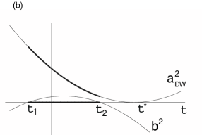
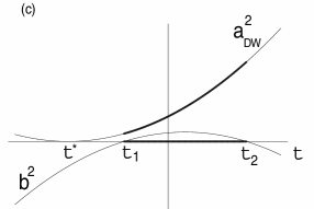
Figure 1: (a) $\Lambda_{B}>0$     ,     (b) $\Lambda_{B}<0$ and $\mu<0$     ,      (c) $\Lambda_{B}<0$ and $\mu>0$

Since in the solution (35)-(36) (as it is also seen from equation (31)) the time-dependent part of $a^{2}$ is exactly $b^{{}^{2}}$, there exists a time parameter $\eta$ (“conformal time”), such that the whole time-dependence $b^{2}(\eta)\equiv b^{2}(t(\eta))$ of the line-element (2) is factorizable, i.e.

$$ds^{2}=b^{2}(\eta)(-d\eta^{2}+dy^{2}+e^{\pm\mu\Lambda_{b}y}\delta_{ij}dx^{i}dx^{j}).$$ (40)

As $t$ approaches the endpoints $t_{1},t_{2}$, the scale factor $b^{2}$ tends to zero. How can a non-zero scale factor of the three-universe exist in this limiting region? This vanishing is characteristic of the foliation of the bulk space defined by the above line-element; the bulk space, as explained in the previous section, is for all times a space of constant curvature. However, the moving three-universe resides in a hypersurface which does not belong to this foliation. So, what we have found is that $a_{DW}(t)\rightarrow$ constant as $t\rightarrow t_{1},t_{2}$, even though $a(t,y)\rightarrow 0$ for any fixed $y$. Further use of the form (40) for the metric will be made in section 5.

As far as proper time $\tau$ is concerned, we get from equations (6), (17) and (39) that

$$a_{DW}^{2}(\tau)=e^{\pm\frac{1}{3}\sqrt{\Lambda_{b}^{2}+6\Lambda_{B}}\,(\tau-\tau_{o})}\,.$$ (41)

The proper time follows $t$ to $\pm\infty$ but remains finite as $t\rightarrow t_{1},t_{2}$ for the case $\Lambda_{B}>0$, while it is still defined in a finite interval for $\Lambda_{B}<0$. Note that the $+$ sign of the preceding expression refers to the cases (i) $\Lambda_{B}<0$ and $\mu>0$, (ii) $\Lambda_{B}>0$ and for the $+\infty$ region solution, while the $-$ sign refers to (iii) $\Lambda_{B}<0$ and $\mu<0$, (iv) $\Lambda_{B}>0$ and for the $-\infty$ region solution. Two more remarks concerning equation (41) are pertinent: (1) This three-universe solution has a “classical” four-dimensional de Sitter form with an “effective” cosmological constant $\Lambda_{dS}=\frac{1}{12}(\Lambda_{b}^{2}+6\Lambda_{B})$. (2) This solution, in contrast to the conventional de Sitter one, does not collapse (see e.g. [16]), a fact that certainly comes from the existence of extra dimensions. Thus, the domain wall with the metric (4) is a portion of $dS_{4}$ space (embedded in $(A)dS_{5}$). The full domain wall extension is the geodesically complete and non-singular $dS_{4}$ space.

In fixed-brane cosmologies, there is an autonomous equation [10] governing the time evolution of the scale factor of the three-universe, which is obtained without having knowledge of the metric outside the brane. On the contrary, in the moving formalism, the exact solution of the bulk space is necessary in order to specify the three-universe evolution, a fact due to the dynamical interaction of the domain wall with the entire space. Furthermore, for a prefixed-position brane, an autonomous induced dynamics on the brane was obtained [17] for an $(A)dS_{5}$ or Minkowski bulk. Although this fact does not concern our procedure, after we have resulted in an $(A)dS_{5}$ bulk, both conclusions must be in agreement. Actually, the matter content of the brane supplied by [17] is exactly our “effective” cosmological constant.

5    Scalar field description

It would be interesting for a further investigation of the physical properties of the bulk metric to consider some tensor perturbations of it. We do not embark on this study here, but instead we deal, in a simplified setting, with the inclusion of a scalar field propagating (but not back-reacting) in the spacetime described by equations (35), (36). Although the bulk background can be cast into a standard $(A)dS_{5}$ form, we believe that the consideration of such a field through the foliation arising from the privileged role played by the three-universe is meaningful. As a starting comment, we recall that it was proved in [12] that the equations governing the transverse traceless fluctuations around the general classical five-dimensional background metric with four-dimensional Poincar$\acute{e}$ symmetry (which is not certainly the situation we intent to investigate) coincide with the equation of motion of a free massless scalar field in the same curved background. In an $AdS_{5}$ black hole background, the spin-2 components of the graviton were also found to obey a free scalar wave equation [18, 19].
The action of our bulk field $\phi(t,y,x^{i})$ is assumed to be

$$S=\frac{1}{2}\int_{M}d^{5}x\sqrt{-g}\,(g^{AB}\partial_{A}\phi\partial_{B}\phi+m^{2}\phi^{2})+\int_{\Sigma}d^{4}x\sqrt{-h}\,\hat{V}(\phi),$$ (42)

where $g=get(g_{AB})$, $h=det(h_{AB})$, $M$ is the full five-dimensional spacetime and $\Sigma$ is the domain wall hypersurface. Setting the variation of the action with respect to $\phi$ equal to zero yields the scalar field equation

$$(\Box-m^{2})\phi=\frac{d\hat{V}}{d\phi}\delta(x^{A}-x^{A}_{DW}),$$ (43)

where $\Box=\frac{1}{\sqrt{-g}}\partial_{A}(\sqrt{-g}\,g^{AB}\partial_{B})$ is the five-dimensional Laplacian. The presence of the delta function in equation (43) is irrelevant for the integration procedure outside $\Sigma$, but it has to be included at the boundary condition on the hypersurface, if one wants to get a global solution. In the same spirit, Israel junction conditions are the boundary conditions for the geometry. The role played by the potential $\hat{V}(\phi)$ appearing in (42) will be explained later. The importance of such surface terms, added to bulk scalar field actions without back-reaction, has been discussed, within the context of fixed-brane cosmologies, in [20] (the back-reaction has been taken into account in [12, 21]). Integrating equation (43) around $\Sigma$, we get the following boundary condition for the continuous field $\phi$:

$$[n^{A}\partial_{A}\phi]=\left(\frac{d\hat{V}}{d\phi}\right)_{wall}\,,$$ (44)

where the bracket denotes, as usual, the discontinuity of the quantity across the domain wall.

We will work out equation (43) using as time-parameter the conformal time $\eta$ of the bulk metric defined in (40). Then, the wave equation can be written as

$$\left(\frac{\partial_{\eta}^{2}\phi}{\phi}+\partial_{\eta}(\ln b^{3})\,\frac{\partial_{\eta}\phi}{\phi}+m^{2}b^{2}\right)-\left(\frac{\phi\,\acute{}\,\acute{}}{\phi}\pm\frac{3}{2}\mu\Lambda_{b}\,\frac{\phi\,\acute{}}{\phi}\right)-e^{\mp\mu\Lambda_{b}y}\,\frac{\delta^{ij}\partial_{i}\partial_{j}\phi}{\phi}=0.$$ (45)

Because of the homogeneity of the spatial sections, the $x$-dependence of the mode solutions are separable, as it is seen from (45), i.e.

$$\phi_{\vec{k}}(\eta,y,x^{i})=(2\pi)^{-\frac{3}{2}}\,e^{i\vec{k}\cdot\vec{x}}\,\tilde{\phi}_{k}(\eta,y),$$ (46)

where $k=(\delta_{ij}k^{i}k^{j})^{\frac{1}{2}}$ and the prefactor in (46) guarantees the standard normalization of its spatial part. Then, the field equation (45) admits separability in $\eta$ and $y$ as well, i.e.

$$\tilde{\phi}_{k}(\eta,y)=u_{k}(\eta)\psi_{k}(y),$$ (47)

where $\psi_{k}$, $u_{k}$ satisfy respectively the equations

$$\frac{\psi_{k}\acute{}\,\acute{}}{\psi_{k}}\pm\frac{3}{2}\mu\Lambda_{b}\,\frac{\psi_{k}\acute{}}{\psi_{k}}-k^{2}\,e^{\mp\mu\Lambda_{b}y}+\lambda=0$$ (48)

$$\frac{\partial_{\eta}^{2}u_{k}}{u_{k}}+\partial_{\eta}(\ln b^{3})\,\frac{\partial_{\eta}u_{k}}{u_{k}}+m^{2}b^{2}+\lambda=0,$$ (49)

with $\lambda$ being a new separation constant. The first of these equations is transformed through a combined change of $y$, $\psi_{k}$ :

$$\bar{y}=\frac{2k}{|\mu\Lambda_{b}|}\,e^{\mp\frac{1}{2}\mu\Lambda_{b}y}\,\,\,,\,\,\,\bar{\psi}_{k}=e^{\pm\frac{3}{4}\mu\Lambda_{b}y}\,\psi_{k},$$ (50)

to the modified Bessel equation

$$\bar{y}^{2}\,\frac{d^{2}\bar{\psi}_{k}}{d\bar{y}^{2}}+\bar{y}\,\frac{d\bar{\psi}_{k}}{d\bar{y}}-(\bar{y}^{2}+\frac{9}{4}-\frac{4\lambda}{\mu^{2}\Lambda_{b}^{2}})\,\bar{\psi}_{k}=0.$$ (51)

The solutions to (51) consist of linear combinations of the modified Bessel functions $I_{\rho}(\bar{y})$, $K_{\rho}(\bar{y})$, where $\rho=\sqrt{\frac{9}{4}-\frac{4\lambda}{\mu^{2}\Lambda_{b}^{2}}}$  .

As a consequence of the signature of the bulk metric $g_{AB}$, the wave operator is hyperbolic. Thus, we do not expect (and even want), square integrability of $\phi$ with respect to time under the hermitian measure of (45). Nevertheless, integrability with respect to $x^{i},\,y$, i.e. on the constant time hypersurfaces, would be desirable. Due to the fact that the classical domain wall motion in the bulk space, as described by the function $y(t)$ of (38), is bounded, $\psi_{k}(y)$ will be normalizable in this compact $y$-range $\mathrm{D}$, with either the flat measure or the natural curved background one $e^{\pm\frac{3}{2}\mu\Lambda_{b}y}$. However, this is not the final word. In the treatments with $y=$constant branes, the three-universe is unfolded in one such hypersurface; no motion takes place, precisely speaking, in the extra dimension, whose existence certainly influences the 3-motion. On the contrary, in our model the true classical motion of the three-universe takes place in an unbounded five-dimensional space. Moreover, having in mind that the classical $\phi$ will have a quantum mechanical analogue, we state that it is more desirable for $\psi_{k}$ to be normalizable in the infinite $y$-range. Of course, the $t$-time range of the bulk solution is $\mathcal{D}$. The functions $I_{\rho}$ , $K_{\rho}$ or any linear combination of them have an exponentially damping behaviour in the neighborhood of one of the two infinities, but not both. The existence of the domain wall can guarantee this normalizability. The boundary condition (44) gives information only for the discontinuity of the normal to the wall component of the gradient of $\phi$. Its parallel components can be either continuous or discontinuous. The existence of $\hat{V}(\phi)$ in (42) and the non-determination of $[\mathrm{e}^{A}\,\partial_{A}\phi]$ from the above condition, allows us to obtain $[\partial_{\eta}u_{k}]=0$ for any $\eta$ and $[\partial_{y}\psi_{k}]\neq 0$ for few or any values of $y\in\mathrm{D}$. As it can be seen from (44), the necessary and sufficient condition for $[\partial_{\eta}u_{k}]=0$ is

$$[\mathrm{e}^{A}\,\partial_{A}\phi]=\frac{\mathrm{e}_{y}}{n_{y}}\left(\frac{d\hat{V}}{d\phi}\right)_{wall}.$$ (52)

Thus, $u_{k}(\eta)$ is differentiable at any instant of time and equation (49) can be investigated further. Then, if $(d\hat{V}/d\phi)_{wall}$ is not identically zero, there exists at least one of the $\psi_{k}$’s with $[\partial_{y}\psi_{k}]\neq 0$, at least at one point $y$. In this way, $\psi_{k}(y)$ is managing to “turn” its slope down and assure normalizability in the infinite $y$-range. More sophisticated situations could arise depending on the form of $(d\hat{V}/d\phi)_{wall}$. It is possible even to obtain functions $\psi_{k}$ continuous in $\mathrm{D}$, nowhere differentiable. The restriction of $\phi$ on the wall (which could be interpreted as the restriction of $\phi$ on our visible universe) will be a continuous function of $t,x^{i}$, possessing non-differentiable in time characteristics due to its part $\psi_{k}(y(t))$.

So much about $\psi_{k}$. Now consider equation (49). Defining the function

$$\bar{u}_{k}=b^{\frac{3}{2}}\,u_{k},$$ (53)

we transform this equation to its canonical form

$$\frac{\partial_{\eta}^{2}\bar{u}_{k}}{\bar{u}_{k}}+\left[\left(m^{2}-\frac{5\Lambda_{B}}{8}\right)b^{2}+\left(\lambda-\frac{9\mu^{2}\Lambda_{b}^{2}}{16}\right)\right]=0,$$ (54)

in which use of equation (33) has been made. We can find from (33) the exact relation between $b$ and $\eta$ to be

$$b(\eta)=\frac{|\mu\Lambda_{b}|}{2}\sqrt{\frac{6}{\Lambda_{B}}}\,\csc h(\mp\frac{|\mu\Lambda_{b}|}{2}\,\eta),$$ (55)

$$b(\eta)=\frac{|\mu\Lambda_{b}|}{2}\sqrt{\frac{6}{|\Lambda_{B}|}}\,\sec h(\frac{|\mu\Lambda_{b}|}{2}\,\eta)$$ (56)

for $\Lambda_{B}>0$ and $\Lambda_{B}<0$ respectively. The $-$ ($+$) sign in (55), with $\eta$-range $(-\infty,0)$ (resp. $(0,+\infty)$), corresponds to the $+\infty$ ($-\infty$) region of the solution (35)-(36), while for $\Lambda_{B}<0$ we have $\eta\in(-\infty,+\infty)$. The above expressions, substituted in equation (54), supply the exact equations for $\bar{u}_{k}$ in $\eta$-time. Making the transformation

$$z=\cosh(\frac{|\mu\Lambda_{b}|}{2}\,\eta)\,\,,\,\,F_{k}=\sinh^{-\frac{1}{2}}(\frac{|\mu\Lambda_{b}|}{2}\,\eta)\,\,\bar{u}_{k}\,,$$ (57)

for $\Lambda_{B}>0$, and

$$z=\cosh(\frac{|\mu\Lambda_{b}|}{2}\,\eta+\frac{i\pi}{2})\,\,,\,\,F_{k}=\cosh^{-\frac{1}{2}}(\frac{|\mu\Lambda_{b}|}{2}\,\eta)\,\,\bar{u}_{k}\,,$$ (58)

for $\Lambda_{B}<0$, equation (54) is converted in both cases to the associated Legendre equation

$$(1-z^{2})\frac{d^{2}F_{k}}{dz^{2}}-2z\frac{dF_{k}}{dz}+\left[\nu(\nu+1)-\frac{\mathrm{m}^{2}}{1-z^{2}}\right]F_{k}=0,$$ (59)

where $\mathrm{m}=(4-\frac{6m^{2}}{\Lambda_{B}})^{\frac{1}{2}}$ , and $\nu(\nu+1)=2-\frac{4\lambda}{\mu^{2}\Lambda_{b}^{2}}$  $(\mathrm{m},\nu\in\mathbf{C})$. It is well known that the general solution of equation (59) consists of linear combinations of Legendre functions of first and second kind, i.e. $P_{\nu}^{\mathrm{m}}(z)$ and $Q_{\nu}^{\mathrm{m}}(z)$ (in our case toroidal functions). Of course, the specific choice of this combination determines the bulk vacuum. Each of these functions carries the real continuous “separation” label $\lambda$, contained in $\nu$, which makes the corresponding $\bar{u}_{k\lambda}$’s (modes) - along with their complex conjugates - complete sets in the space of functions. For example, the state $|\,0\,\rangle_{P}$ defined with respect to the $P$ functions will be inequivalent to the state $|\,0\,\rangle_{Q}$ defined with respect to the modes $Q$.

When $b^{2}\rightarrow 0$, equation (54) is approximated by

$$\frac{\partial_{\eta}^{2}\bar{u}_{k}}{\bar{u}_{k}}+\left(\lambda-\frac{9\mu^{2}\Lambda_{b}^{2}}{16}\right)=0,$$ (60)

which admits for $\lambda>\frac{9\mu^{2}\Lambda_{b}^{2}}{16}$ the “Minkowski-type” modes

$$\bar{u}_{k}^{(\infty)}(\eta)=\frac{1}{\sqrt{2\omega}}\,e^{-i\omega\eta}\,,$$ (61)

where $\omega=\sqrt{\lambda-\frac{9\mu^{2}\Lambda_{b}^{2}}{16}}$  . For $\Lambda_{B}<0$, the regions $b^{2}\rightarrow 0$ are the two asymptotic regions of (56) as $\eta\rightarrow\pm\infty$. The modes $\bar{u}_{k}$ that behave like positive frequency modes (61) in these limits, i.e. $\bar{u}_{k}(\eta)\rightarrow\bar{u}_{k}^{(\infty)}(\eta)$ as $\eta\rightarrow\pm\infty$, are

$$\bar{u}_{k}(\eta)=\frac{(-1)^{-\frac{1}{2}\mathrm{m}}\,i^{\nu+\mathrm{m}+1}}{\sqrt{\pi\omega}\,e^{i\mathrm{m}\pi}}\frac{\Gamma(\nu+\frac{3}{2})}{\Gamma(\nu+\mathrm{m}+1)}\cosh^{\frac{1}{2}}(\frac{|\mu\Lambda_{b}|}{2}\eta)\,Q_{\nu}^{\mathrm{m}}(i\sinh(\frac{|\mu\Lambda_{b}|}{2}\eta)).$$ (62)

This expression holds for $\eta>0$ (“out” modes), while for $\eta<0$ (“in” modes) it has to be multiplied by $(-1)^{\nu-\mathrm{m}}$. For $\eta>0$, Im$\nu>0$ is used, while for $\eta<0$, Im$\nu<0$. Vacuum states defined in similar ways have been given in [22, 23]. For the derivation of equation (62) the defining relation of  $Q_{\nu}^{\mathrm{m}}(z)$  in terms of  ${}_{2}F_{1}\,(1+\frac{1}{2}\,(\nu+\mathrm{m}\,)\,,\,\frac{1}{2}\,(1+\nu+\mathrm{m}\,)\,;\,\nu+\frac{3}{2}\,;\,\frac{1}{z^{2}})$ ,  $|z|>1$ has been used (see [24], p. 332). The modes $\bar{u}_{k}^{in}$, $\bar{u}_{k}^{out}$ are connected through a Bogolubov transformation, thus, if the quantum state is chosen to be $|\,0\,\rangle_{in}$, an unaccelerated particle detector in the out region will detect some spectrum. Of course, the detector is considered to move in the bulk space and the particle creation occurs in this space due to the bulk cosmological evolution. Further examination of the situation would require the evaluation of the Wightman function in the out region constructed using the in vacuum.

It holds that $|\partial_{\eta}(\ln b^{2})|\rightarrow|\mu\Lambda_{b}|$ as $\eta\rightarrow\infty$ and $\partial_{\eta}(\ln b^{2})\rightarrow\infty$ as $\eta\rightarrow 0$. Thus, since our spacetime is not slowly expanding in the two asymptotic limits, we cannot define physically reasonable adiabatic in and out vacua. Although adiabatic in and out regions do not exist, it is still possible to define adiabatic vacua as being those which are vacuous in the high label $\lambda$ modes. Recall [25] that for the case of our harmonic oscillator-type equation (54) (with time-dependent frequency), the “zeroth order adiabatic modes”

$$\bar{u}_{k}^{(0)}(\eta)=\frac{1}{\sqrt{2}\,\,\Omega_{\lambda}^{1/4}(\eta)}\,e^{-i\int^{\eta}\Omega_{\lambda}^{1/2}(\eta^{\prime})d\eta^{\prime}},$$ (63)

where $\Omega_{\lambda}(\eta)=(\lambda-\frac{9\mu^{2}\Lambda_{b}^{2}}{16})+(m^{2}-\frac{5\Lambda_{B}}{8})b^{2}(\eta)$, become good approximations to exact adiabatic positive frequency modes, when the quantity

$$T^{2}\Omega_{\lambda}(\eta_{1})=T^{2}\left(\lambda-\frac{9\mu^{2}\Lambda_{b}^{2}}{16}\right)\pm T^{2}\,\frac{3\mu^{2}\Lambda_{b}^{2}}{2}\left(\frac{m^{2}}{\Lambda_{B}}-\frac{5}{8}\right)\csc h^{2}\left(\frac{|\mu\Lambda_{b}|}{2}\,\eta_{1}T\right)$$ (64)

- with $T$ being the so-called adiabatic parameter and $\eta_{1}=\frac{\eta}{T}$ - becomes large with respect to the derivatives of $\partial_{\eta}\ln b^{2}=$O$(T^{-1})$ for fixed $\eta_{1}$. This is the case for large $\lambda$ or large $m^{2}/|\Lambda_{B}|$ (but not for small $|\eta|$), either individually or together. In (64) the $+\,(-)$ sign corresponds to $\Lambda_{B}>0\,(<0)$ and the $\csc h$ has to be replaced by $\sec h$ in the $\Lambda_{B}<0$ case. The above described picture resembles somehow the common 4-dimensional quantum theory of de Sitter space, where the trigonometric functions have been replaced by hyperbolic ones. In the limit of large $\lambda$ with $\mathrm{m}$, $\mu\Lambda_{b}$ and $\eta$ fixed, we have  $\Omega_{\lambda}(\eta)\simeq\lambda$, which, when substituted in (63), gives

$$\bar{u}_{k}^{(0)}(\eta)\rightarrow\frac{1}{\sqrt{2}\,\lambda^{\frac{1}{4}}}\,e^{-i\sqrt{\lambda}\,\eta}\,.$$ (65)

For $\Lambda_{B}>0$, the choice

$$\bar{u}_{k}(\eta)= \frac{(\nu+\frac{1}{2})^{\frac{1}{2}-\mathrm{m}}}{2^{2\mathrm{m}+1}\,\lambda^{\frac{1}{4}}}\,\frac{\Gamma(1-\mathrm{m})\,\Gamma(\frac{1}{2}-\mathrm{m})}{f\,\Gamma(1-2\mathrm{m})}\,\sinh^{\frac{1}{2}}(\frac{|\mu\Lambda_{b}|}{2}\eta)\,[\frac{f-1}{\sin(\mathrm{m}\pi)}\,P_{\nu}^{\mathrm{m}}(\cosh(\frac{|\mu\Lambda_{b}|}{2}\,\eta))+$$ (66)

$$\,\,\,\,\,\,\,\,\,\,\,\,\,\,\,\,\,\,\,\,\,\,\,\,\,\,\,\,\,\,\,\,\,\,\,\,\,\,\,\,\,\,\,\,\,\,\,\,\,\,\,\,\,\,\,\,\,\,\,\,\,\,\,\,\,\,\,\,\,\,\,\,\,\,\,\,\,\,\,\,\,\,\,\,\,\,\,\,\,\,\,\,\,\,\,\,+\frac{2}{\pi}\,e^{-i\mathrm{m}\pi}\,Q_{\nu}^{\mathrm{m}}(\cosh(\frac{|\mu\Lambda_{b}|}{2}\,\eta))],$$

where $f=\frac{1}{2^{4\mathrm{m}}(\nu+\frac{1}{2})^{2\mathrm{m}}}\,\frac{\Gamma(1-\mathrm{m})\,\Gamma(\frac{1}{2}-\mathrm{m})\,\Gamma(1+2\mathrm{m})\,\Gamma(\nu+\mathrm{m}+1)}{\Gamma(1-2\mathrm{m})\,\Gamma(1+\mathrm{m})\,\Gamma(\frac{1}{2}+\mathrm{m})\,\Gamma(\nu-\mathrm{m}+1)}$   and  Im$\nu>0$, has the property

$$\bar{u}_{k}(\eta)\rightarrow\bar{u}_{k}^{(0)}(\eta)\,\,,\,\,\lambda\rightarrow+\infty.$$ (67)

This solution refers to the $+\infty$ region; for the $-\infty$ region the above $\bar{u}_{k}$ has to be multiplied by $-i$. For the derivation of the relation (67) the following equations have been used:
i) $P_{\nu-\frac{1}{2}}^{\nu\,\acute{}}(\cosh x)=\frac{2^{2\nu\,\acute{}}}{\Gamma(1-\nu\,\acute{}\,)}(1-e^{-2x})^{-\nu\,\acute{}}\,e^{-(\nu+\frac{1}{2})x}\,_{2}F_{1}(\frac{1}{2}-\nu\,\acute{}\,\,,\,\frac{1}{2}+\nu-\nu\,\acute{}\,\,;\,1-2\nu\,\acute{}\,\,;1-e^{-2x})$
(see [24], p. 336)
ii) ${}_{2}F_{1}(a,b+r;c;z)=\frac{\Gamma(c)}{\Gamma(a)\,\Gamma(c-a)}\,\{\Gamma(c-a)\,(rz)^{a-c}\,(1-z)^{c-a-b-r}\,[1+$O$(r^{-1})]\,+$
$\,\,\,\,\,\,\,\,\,\,\,\,\,\,\,\,\,\,\,\,\,\,\,\,\,\,\,\,\,\,\,\,\,\,\,\,\,\,\,\,\,\,\,\,\,\,\,\,\,\,\,\,\,\,\,\,\,\,\,\,\,\,\,\,\,\,\,\,\,\,\,\,\,\,\,\,\,\,\,\,\,\,\,+\Gamma(a)\,(rz\,e^{-i\pi})^{-a}\,[1+$O$(r^{-1})]\,\}\,\,,\,\,\,\,\,\,\,|r|\rightarrow\infty$
(see [26], vol. 1, p. 241) and also the relation between $Q_{\nu}^{\mathrm{m}}$ and $P_{\nu}^{\mathrm{m}}$, $P_{\nu}^{\mathrm{-m}}$. Equation (66) diverges for $\mathrm{m}\in\mathbf{Z}$, since $\sin(\mathrm{m}\pi)$ vanishes. The massless field $m=0$ is included in this case. For a negative cosmological constant $\Lambda_{B}$, an adiabatic vacuum cannot be defined using the above approximations. Since the solution (66) reduces to (65) in the limit of large $\lambda$, regardless of the value of $\eta$ (see [27]), it defines a stable adiabatic vacuum for all times. Thus, the modes (66) are positive frequency with respect to the adiabatic definition, and in this vacuum an inertial detector registers no particles.

6    Conclusions

Recently, there has been renewed interest in cosmological models with extra dimensions. Major effort has been devoted to branes sitting on fixed positions of the bulk space. In this work, we have investigated the existence of bulk solutions arising from a moving domain wall framework. In the beginning we derived, based on the Israel matching conditions, the equations governing a moving domain wall in a general class of cosmological bulk metrics. Subsequently, assuming an ansatz for these metrics consisting of true time-dependence of the two “lapse” functions, we were in a position to obtain an additional first integral for the domain wall motion when the matter on the wall is a cosmological constant. This leads to a condition (unique for only one scale factor of the $D-2$ part) between the bulk metric components, necessary for the compatibility of the formalism. Afterwards, we found for a flat three-universe, a five-dimensional three-parameter bulk solution admitting the above described wall motion, when a cosmological constant exists in the whole spacetime. This solution is shown to be the unique solution under the conditions assumed. Investigating the properties of this bulk space, we saw that locally it is simply the well known $dS_{5}$ or $AdS_{5}$ space. Hence, these spaces admit moving three-universes whose trajectories are determined by the found solution. The domain wall formed by the motion of the three-universe corresponds to the “physical” four-dimensional spacetime. This is shown to be $dS_{4}$. A remarkable fact concerning this three-universe is that its scale factor does not vanish during its unfolding through the bulk space, i.e. it avoids collapsing. As the conformal time goes to infinity, this scale factor reaches a positive minimum, and the bulk metric has an apparent (coordinate) singularity there. If another foliation of the $(A)dS_{5}$ space is adopted, avoiding this singularity, then the fate of the corresponding three-universe should be examined anew.

For negative bulk cosmological constant, the bulk space being $AdS_{5}$, the metric could be cast in the form appearing in [8, 12], with the emergence of a bound gravitational state. Our solution corresponds to a three-universe that does not reside in a prefixed-position brane. The two pictures correspond to distinct physical situations and do not seem to be continuously connected.

As an application of the properties the above bulk metric possess, we considered the inclusion of a scalar field, neglecting its back-reaction on the background. The wave equation of the scalar field is separable and its complete solution has been obtained. The inclusion of a general domain wall, coupled to the field, can guarantee the normalizability of the field in the infinite extra-dimension range. The time-dependent part of the field, examined in the “conformal” gauge, allows, for a negative bulk cosmological constant, the definition of asymptotically positive frequency behaved modes, even in the massless limit. For positive cosmological constant an adiabatic vacuum has been consistently defined for non-zero mass. Notions of particle creation in the bulk space can be extracted, though this topic deserves further investigation.

It seems interesting and also possible to find a 4-parameter solution containing $\mathcal{C}\neq 0$ and/or a non-flat three universe. A harder task would be to find any solutions with the “lapses” being functions of both time and the extra coordinate. The inclusion of two different bulk cosmological constants in the two sides of the domain wall, relaxing the reflection symmetry assumption would also be interesting, within string or supergravity theory, for whatever ansatz of the bulk metric. Furthermore, a perfect fluid content in the three-universe would make a moving domain wall model cosmologically more realistic. Finally, we refer to the work [28], where a self-inflationary solution was introduced, which produces a phase of late accelerated expansion, as indicated by recent supernova data. This is the result of an intrinsic curvature Ricci scalar, included in the brane action. It would be desirable if one managed to embody such a geometric term in the Israel conditions of the moving formalism.

References

- [1] A. Kehagias and E. Kiritsis, “Mirage cosmology”, JHEP 9911 (1999) 022, hep-th/9910174.
- [2] H.A. Chamblin and H.S. Reall, “Dynamic dilatonic domain walls”, Nucl. Phys. B562 (1999) 133, hep-th/9903225.
- [3] A. Chamblin, M.J. Perry and H.S. Reall, “Non-BPS D8-branes and dynamic domain walls in massive IIA supergravities”, JHEP 9909 (1999) 014, hep-th/9908047.
- [4] W. Israel, “Singular hypersurfaces and thin shells in General Relativity”, Nuovo Cimento 44B (1966) 1; erratum, Nuovo Cimento 49B (1967) 463.
- [5] P. Kraus, “Dynamics of anti-de Sitter domain walls”, JHEP 9912 (1999) 011, hep-th/9910149.
- [6] C. Park and S.J. Sin, “Moving domain walls in and graceful exit from inflation”, Phys. Lett. B485 (2000), hep-th/0005013.
- [7] N. Arkani-Hamed, S. Dimopoulos and G. Dvali, “The hierarchy problem and new dimensions at a milimeter”, Phys. Lett. B429 (1998) 263, hep-ph/9803315.
- [8] L. Randall and R. Sundrum, “A large mass hierarchy from a small extra dimension”, Phys. Rev. Lett. 83 (1999) 3370, hep-ph/9905221; “An alternative to compactification”, Phys. Rev. Lett. 83 (1999) 4690, hep-th/9906064.
- [9] D.N. Vollick, “Cosmology on a three-brane”, Class. Quant. Grav. 18 (2001) 1, hep-th/9911181.
- [10] P. Bintruy, C. Deffayet, U. Ellwanger, D. Langlois, “Brane cosmological evolution in a bulk with cosmological constant”, Phys. Lett. B477 (2000) 285, hep-th/9910219.
- [11] R.N. Mohapatra, A. Prez-Lorenzana and C.A. de S. Pires, “Cosmology of brane-bulk models in five dimensions”, Int. J. Mod. Phys. A16 (2001) 1431, hep-ph/0003328.
- [12] O. DeWolfe, D.Z. Freedman, S.S. Gubser, A. Karch, “Modeling the fifth dimension with scalars and gravity”, Phys. Rev. D62 (2000) 046008, hep-th/9909134.
- [13] J.P. de Leon, “Cosmological models in a Kaluza-Klein theory with variable rest mass”, Gen. Rel. Grav. 20 (1988) 6.
- [14] M.P. Ryan and L.C. Shepley, “Homogeneous Relativistic Cosmologies”, Princeton University, Princeton, New Jersey (1975).
- [15] M. Spivak, “A comprehensive Introduction of Differential Geometry”, vol. 4, Publish or Perish, Inc. (1975).
- [16] S.W. Hawking and G.F.R. Ellis, “The large scale structure of space-time”, Cambridge University Press (1973).
- [17] T. Shiromizu, K. Maeda and M. Sasaki, “The Einstein equations on the 3-Brane World”, Phys. Rev. D62 (2000) 024012, gr-qc/9910076.
- [18] N.R. Constable, N.C. Myers, “Spin two glueballs, positive energy theorems and the ADS/CFT correspondence”, JHEP 10 (1999) 037, hep-th/9908175.
- [19] R.C. Brower, S.D. Mathur, C.I. Tan, “Discrete spectrum of the graviton in the black hole background”, Nucl. Phys. B574 (2000) 219, hep-th/9908196.
- [20] W.D. Goldberger and M.B. Wise, “Modulus stabilization with bulk fields”, Phys, Rev. Lett. 83 (1999) 4922, hep-ph/9907447.
- [21] N. Tetradis, “On brane stabilization and the cosmological constant”, Phys. Lett. B509 (2001) 307, hep-th/0012106.
- [22] H. Rumpf, Phys. Lett. 61B (1976) 272; Nuovo Cimento 35B (1976) 321.
- [23] J.S. Dowker and R. Critchley, Phys. Rev. D13 (1976) 224.
- [24] M. Abramowitz and I.A. Stegun, “Handbook of mathematical functions”, Dover Pbs.
- [25] N.D. Birrell and P.C.W. Davies, “Quantum fields in curved space”, Cambridge University Press (1982).
- [26] Y.L. Luke, “The special functions and their approximations”, Academic Press (1969).
- [27] N.A. Chernikov and E.A. Tagirov, Ann. Inst. Henri Poincar 9A (1968) 109.
- [28] C. Deffayet, “Cosmology on a brane in Minkowski bulk”, Phys. Lett. B502 (2001) 199, hep-th/0010186.