On the correspondence between D-branes and stationary supergravity solutions of type II Calabi-Yau compactifications.

Abstract:

In this talk, I review how four dimensional stationary supergravity solutions that are more general than spherically symmetric black holes emerge naturally in the low energy description of BPS states in type II Calabi-Yau compactifications. An explicit construction of multicenter solutions using single center attractor flows as building blocks is presented, and some interesting properties of these solutions are examined. We end with a brief remark on non-BPS configurations.

1 Introduction

Calabi-Yau compactifications of type II string theory, which have ${\mathcal{N}}=2$ residual supersymmetry in four dimensions, are known to have a moduli dependent spectrum of wrapped BPS D-branes; such branes, observed as BPS particles in four dimensions, can for example decay at so-called surfaces of marginal stability, similar to the well known decays of BPS particles in Seiberg-Witten theory [1]. In type IIB theory, when the geometric D-brane picture can be trusted, the mathematical equivalent of existence of a BPS brane in a certain homology class, is the existence of a special lagrangian submanifold in that class. In recent years, the latter problem got quite some attention, though it turned out to be an extremely difficult issue [2, 3], and the general existence question remains largely unsolved. In type IIA theory, the mathematical equivalent is the existence of certain holomorphic bundles on holomorphic submanifolds, again when the geometric D-brane picture can be trusted. This problem is better under control, though our understanding is far from complete. Existence of BPS states in stringy regimes of the moduli space, such as the Gepner point of the Quintic, can in favorable circumstances be tackled from a pure conformal field theory perspective, building on the work of [4]. Substantial work in this context has been pioneered in [5] and significantly extended in [6, 7, 8, 9, 10, 11, 12, 13, 14].

From a complementary, four dimensional low energy point of view, one expects to have BPS solutions to the supergravity equations of motion for any BPS state in the spectrum, at least if supergravity can be trusted. The simplest solutions of this kind are spherically symmetric black holes. Those were first studied in ${\mathcal{N}}=2$ theories in [15], where it was shown that they exhibit a remarkable “attractor” feature: the value of the moduli at the horizon are fixed by the charge of the black hole, in the sense that they are invariant under continuous changes of the moduli at infinity. In [16], where this property was linked to a vast and still largely unexplored treasure of arithmetical properties, it was noted that the existence of these solutions is a nontrivial problem, depending strongly on the value of the charges and vacuum moduli. It is therefore natural to conjecture [16] a correspondence between the existence of those supergravity solutions and the existence of BPS D-brane states in the full string theory.

However, as pointed out in [6, 17], this conjecture fails in a number of established cases, where the state is known to exist in string theory, but the corresponding black hole solution does not exist in the supergravity theory, even in regimes where supergravity can clearly be trusted. Obviously, from the physics point of view, this is a major consistency problem.

The solution to this paradox was discovered in [17]: the restriction to spherically symmetric black holes turned out to be too narrow. For one, solutions corresponding to branes wrapped around conifold cycles, though still spherically symmetric, are not black holes, but rather “empty holes”, as a result of a mechanism reminiscent of the enhançon mechanism of [18], with a core carrying instead of a massless vector multiplet and enhanced gauge symmetry, a massless hypermultiplet. But more importantly, ${\mathcal{N}}=2$ supergravity allows for solutions involving mutually nonlocal charges at rest at a finite equilibrium distance from each other. Those solutions are in general stationary but non-static, as they can carry a (quantized) intrinsic angular momentum, much like the monopole-electron system in ordinary Maxwell theory. And as it happens, some of the BPS states found in string theory can only be realized in the low energy theory as such multi-center solutions.

General stationary solutions of four dimensional ${\mathcal{N}}=2$ supergravity were first explored in [19], further analyzed from a geometrical point of view in [17], and given a rigorous, systematic treatment, including $R^{2}$ corrections, in [20].

The multicenter configurations also give a beautiful low energy picture of what happens at marginal stability: the state can literally be seen to decay smoothly into its constituents. Furthermore, Joyce’s stability criterion for special lagrangian submanifolds [2] is elegantly recovered and generalized, and a strong similarity to the general Pi-stability criterion proposed in [10] emerges.

This opens up the exciting possibility that the existence conjecture of [16], suitably generalized to include multicenter solutions, should be taken seriously. The consequences for mathematics and string theory of this correspondence, provided it is true, are clearly far reaching. For example, it would enable us to study the D-brane spectrum of compact Calabi-Yau compactifications (and its mathematical equivalents), in a quite systematic way, a problem that has been pretty elusive thus far using other approaches. This issue, for type IIA theory on the Quintic, will be addressed in a forthcoming paper [21], mainly from a numerical perspective.

In this talk, I will review how solutions more general than spherically symmetric black holes arise in the low energy description of BPS states, focusing on the solutions to the BPS equations rather than on the technicalities of their derivation, for which we refer to [17]. A detailed construction of multicenter solutions from single center flows, a closer examination of some properties of these solutions and a brief digression on non-BPS states, extend the results of this reference.

2 Geometry of IIB/CY compactifications

To establish our notation and setup, let us briefly review the low energy geometry of type-IIB string theory compactified on a Calabi-Yau 3-fold. We will always work in the type IIB framework, but the equivalence with type IIA through mirror symmetry will be implicitly assumed in the presentation of our examples.

We will follow the manifestly duality invariant formalism of [16]. Consider type-IIB string theory compactified on a Calabi-Yau manifold $X$. The four-dimensional low energy theory is ${\mathcal{N}}=2$ supergravity coupled to $n_{v}=h^{1,2}$ massless abelian vectormultiplets and $n_{h}=h^{1,1}+1$ massless hypermultiplets, where the $h^{i,j}$ are the Hodge numbers of $X$. The hypermultiplet fields will play no role in the following and are set to zero.

The vectormultiplet scalars are given by the complex structure moduli of $X$, and the lattice of electric and magnetic charges is identified with $H^{3}(X,\mathbb{Z})$, the lattice of integral harmonic $3$-forms on $X$. The “total” electromagnetic field strength ${\mathcal{F}}$ is (up to normalisation convention) equal to the type-IIB self-dual five-form field strength, and is assumed to have values in $\Omega^{2}(M_{4})\otimes H^{3}(X,\mathbb{Z})$, where $\Omega^{2}(M_{4})$ denotes the space of 2-forms on the four-dimensional spacetime $M_{4}$. The usual components of the field strength are retrieved by picking a symplectic basis ${\alpha^{I},\beta_{I}}$ of $H^{3}(X,\mathbb{Z})$:

$${\mathcal{F}}=F^{I}\otimes\beta_{I}-G_{I}\otimes\alpha^{I}\,.$$ (1)

A 3-brane wrapped around a cycle Poincarè dual to $\Gamma\in H^{3}(X,\mathbb{Z})$ has electric and magnetic charges equal to its components with respect to this basis. The total field strength satisfies the self-duality constraint: ${\mathcal{F}}=*_{10}{\mathcal{F}}\$, which translates to electric-magnetic duality in the four dimensional theory.

The geometry of the vector multiplet moduli space, parametrized with $n_{v}$ coordinates $z^{a}$, is special Kähler [22]. The (positive definite) metric

$$g_{a\bar{b}}=\partial_{a}\bar{\partial}_{\bar{b}}{\mathcal{K}}$$ (2)

is derived from the Kähler potential

$${\mathcal{K}}=-\ln\left(i\int_{X}\Omega_{0}\wedge\bar{\Omega}_{0}\right),$$ (3)

where $\Omega_{0}$ is the holomorphic $3$-form on $X$, depending holomorphically on the complex structure moduli. It is convenient to introduce also the normalized 3-form

$$\Omega=e^{{\mathcal{K}}/2}\,\Omega_{0}\,.$$ (4)

The “central charge” of $\Gamma\in H^{3}(X,\mathbb{Z})$ is given by

$$Z(\Gamma)\equiv\int_{X}\Gamma\wedge\Omega\equiv\int_{\Gamma}\Omega\,,$$ (5)

where we denoted, by slight abuse of notation, the cycle Poincaré dual to $\Gamma$ by the same symbol $\Gamma$. Note that $Z(\Gamma)$ has nonholomorphic dependence on the moduli through the Kähler potential.

We will make use of the (antisymmetric, topological, moduli independent) intersection product:

$$\langle\Gamma_{1},\Gamma_{2}\rangle=\int_{X}\Gamma_{1}\wedge\Gamma_{2}=\#(\Gamma_{1}\cap\Gamma_{2})\,.$$ (6)

With this notation, we have for a symplectic basis $\{\alpha^{I},\beta_{I}\}$ by definition $\langle\alpha^{I},\beta_{J}\rangle=\delta^{I}_{J}$. Integrality of this intersection product is equivalent to Dirac quantization of electric and magnetic charges.

3 BPS equations of motion

3.1 The static, single center, spherically symmetric case

The BPS equations of motion for the static, spherically symmetric case were derived in [15], and cast in the form of first order flow equations on moduli space in [23]. We assume a charge $\Gamma\in H^{3}(X,\mathbb{Z})$ is located at the origin of space. The spacetime metric is of the form

$$ds^{2}=-e^{2U}dt^{2}+e^{-2U}dx^{i}dx^{i}\,,$$ (7)

with $U$ a function of the radial coordinate distance $r=|\bf{x}|$, or equivalently of the inverse radial coordinate $\tau=1/r$. The BPS equations of motion for $U(\tau)$ and the moduli $z^{a}(\tau)$ are:

$$\partial_{\tau}U = -e^{U}|Z|\,,$$ (8)

$$\partial_{\tau}z^{a} = -2e^{U}g^{a\bar{b}}\,\bar{\partial}_{\bar{b}}|Z|\,,$$ (9)

where $Z=Z(\Gamma)$ is as in (5) and $g_{a\bar{b}}$ as in (2). A closed expression for the electromagnetic field, given the solutions of these flow equations, can be found e.g. in [17].

This is the form of the BPS equations found in [23]. An alternative form of the equations, essentially equivalent to those found in [15], is:

$$2\,\partial_{\tau}\left[e^{-U}\mathop{\rm Im}\nolimits\left(e^{-i\alpha}\Omega\right)\right]=-\Gamma\,,$$ (10)

where $\alpha=\arg Z$, which can be shown to be the phase of the conserved supersymmetry (see e.g. [20]). Note that this nice compact equation actually has $2n_{v}+2$ real components, corresponding to taking intersection products with the $2n_{v}+2$ elements of a basis $\{C_{L}\}_{L}$ of $H^{3}(X,\mathbb{Z})$:

$$2\,\partial_{\tau}\left[e^{-U}\mathop{\rm Im}\nolimits\left(e^{-i\alpha}Z(C_{L})\right)\right]=-\langle C_{L},\Gamma\rangle\,,$$ (11)

One component is redundant, since taking the intersection product of (10) with $\Gamma$ itself produces trivially $0=0$. This leaves $2n_{v}+1$ independent equations, matching the number of real variables $\{U,\mathop{\rm Re}\nolimits z^{a},\mathop{\rm Im}\nolimits z^{a}\}$.

Note that alternatively, we could have left $\alpha$ as an arbitrary field instead of putting it equal to $\arg Z$. Then the previously redundant component of the equation gives $\mathop{\rm Im}\nolimits(e^{-i\alpha}Z)=0$, hence $\alpha=\arg Z$ or $\alpha=\arg(-Z)$. The latter possibility is automatically excluded however, since it gives rise to a highly singular, unphysical solution. Indeed, this case corresponds to (8)-(9) with the sign of the right hand sides reversed. Then $|Z|$ and $e^{U}$ would be increasing functions in $\tau$, with $e^{U}$ satisfying the estimate $e^{U}\geq\frac{e^{U(\tau_{0})}}{1-e^{U(\tau_{0})}|Z(\tau_{0})|(\tau-\tau_{0})}$ for any $\tau_{0}$ and $\tau>\tau_{0}$. Since this diverges at finite $\tau$, the solution breaks down. Note that this candidate solution in any case would have had negative ADM mass and be gravitationally repulsive — physically quite undesirable properties. So only the possibility $\alpha=\arg Z$ remains, bringing us back to the original setup of the equations.

Since the right hand side of (11) consists of $\tau$-independent integer charges, (10) readily integrates to

$$2\,e^{-U}\mathop{\rm Im}\nolimits\left(e^{-i\alpha}\Omega\right)=-\Gamma\,\tau+2\mathop{\rm Im}\nolimits\left(e^{-U}e^{-i\alpha}\Omega\right)_{\tau=0}.$$ (12)

For asymptotically flat space, $U_{\tau=0}=U_{r=\infty}=0$.

In contrast to [15] and most of the older attractor literature, we prefer to work with the normalized periods and an explicit phase factor $e^{i\alpha}$. The difference amounts to nothing more than a normalization gauge choice, but it proves to be conceptually more transparent, and numeric-computationally far more convenient to make the above choice.

The result (12) is very powerful, as it solves in principle the equations of motion. Of course, finding the explicit flows in moduli space from (12) requires inversion of the periods to the moduli, which in general is not feasible analytically. However, in large complex structure approximations or numerically for e.g. the quintic, this turns out to be possible.

There is one catch to (12) though, namely, as shown in [17], it is not valid for a vanishing cycle $\Gamma$, at values of the moduli where it vanishes. Indeed, looking for example at a one modulus case near a conifold point, we see that while (8)-(9) allows for solutions with constant $z$ and $U$ at the conifold point (since the inverse metric becomes zero there), this is not the case for (12). The correct equation in this case is (8)-(9). This subtlety is important in the discussion of “empty hole” solutions (see below), and it thus eliminates some confusion in the older attractor literature, where solutions with charge corresponding to a conifold cycle seemed to emerge that were very unphysical (naked curvature singularities, gravitational repulsion, etc.). Such pathological behavior is indeed what one gets when naively applying (12) to those cases.

Finally, it was also observed in [17] that the BPS equations of motion can be interpreted as geodesic equations for stretched strings with varying tension in a certain curved background, making contact, at least in a rigid (gravity decoupling) limit of the theory, with the “3-1-7” brane picture of BPS states in ${\mathcal{N}}=2$ quantum field theory [24, 25].

3.2 The general stationary case

The BPS equations of motion for the general case, though of course more complicated, are quite similar in structure to those of the single center case. For a derivation, we refer to  [17] and  [20]. In the latter reference, the equations below were shown to describe the most general stationary BPS solutions, provided a certain ansatz was made for the embedding of the residual supersymmetry. More general solutions could exist, but a fully general analysis proved to be too cumbersome to be carried out thus far.

The metric will be of the form

$$ds^{2}=-e^{2U}\left(dt+\omega_{i}dx^{i}\right)^{2}+e^{-2U}dx^{i}dx^{i}\,,$$ (13)

where $U$ and $\omega$, together with the moduli fields $z^{a}$, are time-independent solutions of the following BPS equations, elegantly generalizing (12):

$$2\,e^{-U}\mathop{\rm Im}\nolimits\left(e^{-i\alpha}\Omega\right) = H\,,$$ (14)

$$\boldsymbol{*}d\omega = \langle dH,H\rangle\,,$$ (15)

with $H({\bf x})$ an $H^{3}(X)$-valued harmonic function (on flat coordinate space $\mathbb{R}^{3}$), and $\boldsymbol{*}$ the flat Hodge star operator on $\mathbb{R}^{3}$. For $N$ charges $\Gamma_{p}$ located at coordinates ${\bf x}_{p}$, $p=1,\ldots,N$, in asymptotically flat space, one has:

$$H=-\sum_{p=1}^{N}\Gamma_{p}\,\tau_{p}\,\,+\,2\mathop{\rm Im}\nolimits\left(e^{-i\alpha}\Omega\right)_{r=\infty}\,,$$ (16)

with $\tau_{p}=1/|{\bf x}-{\bf x}_{p}|$.

Note that at large $r$, equation (14) reduces to lowest order in $1/r$ to the spherically symmetric case (12). The phase $\alpha$ in (14) is to be considered as an a priori independent unknown field here. However, a reasoning similar to the comments under (11) shows that it must be asymptotically equal to the phase of $Z(\sum_{p}\Gamma_{p})$ for $|{\bf x}|\to\infty$.

The electromagnetic field is again determined algebraically from the solutions of the BPS equations for $U$, $\omega$ and $z^{a}$. We refer to [17] (or [20]) for the explicit expressions.

4 Solutions

4.1 Static single center case: black, empty and no holes.

In asymptotically flat space (which we will assume unless stated otherwise), all well-behaved solutions to to (8)–(9) saturate the BPS bound $M_{ADM}=|Z_{\tau=0}|$. Another simple universal characteristic is that the “size” of the solutions scales proportional to the charge number, due to a trivial rescaling symmetry of the equations of motion. An important and less trivial general property is the following. Equation (9) implies $\partial_{\tau}|Z|=-4e^{U}g^{a\bar{b}}\,\partial_{a}|Z|\,\bar{\partial}_{\bar{b}}|Z|\leq 0$. Therefore the flows in moduli space for increasing $\tau$, given by the BPS equations, will converge to minima of $|Z|$, and the corresponding moduli values are generically invariant under continuous deformations of the moduli at spatial infinity, so they only depend on the charge $\Gamma$, a phenomenon referred to as the attractor mechanism. One distinguishes three cases [16], depending on the value of the minimum of $|Z|$ (zero or nonzero) and its position in moduli space (at singular or regular point):

1. nonzero minimal $|Z|$. This yields a regular BPS black hole. The near-horizon geometry is $AdS_{2}\times S^{2}$, and the horizon area equals $4\pi|Z|^{2}_{min}$. From the BPS equations of motion, one directly deduces that at the horizon, $2\mathop{\rm Im}\nolimits(\bar{Z}\Omega)=-\Gamma$. This equation, determining (locally) the position of the attractor point in moduli space, is often called the attractor equation.

2. zero minimal $|Z|$ at a regular point in moduli space. In this case, the BPS equations do not have a solution [16]: $Z=0$ will be reached by the flow at a finite radius, beyond which the solution cannot be continued. This is consistent with physical expectations: in a vacuum close to a regular zero of $Z$ in moduli space, the state cannot exist, as it would imply the existence of a massless particle at the zero locus, which in turn should create a singularity in moduli space [26], in contradiction with the supposed regularity of the point under consideration.

   

   Figure 1: Energy density sketch of an empty hole.

3. zero minimal $|Z|$ at a singular or boundary point in moduli space. In this case, the BPS equations may or may not have a solution. In the case of a conifold cycle for example, the equations do have a solution, describing an “empty hole” [17]: again, the zero of $Z$ (i.e. the conifold locus in moduli space) is reached at finite radius, but now, as mentioned at the end of section 3.1, the solution can be continued in a ($1\times$) continuous differentiable way, simply as flat space (i.e. constant $U$) with the moduli fixed at the conifold locus. This is illustrated in fig. 1. Inside this core, a test conifold particle would be massless, and the charge source becomes completely delocalized. The latter is illustrated for example by the fact that the core radius of an emty hole increases when the background moduli approach the conifold radius (since the flow reaches the attractor point “earlier” in $\tau$). Therefore, if we let another conifold particle approach our initial empty hole, the radius of that particle will increase, eventually smoothly “melting” into the original core (this process can in fact be analyzed quantitively by considering multicenter solutions with parallel charges).

   All this is quite similar to the enhançon mechanism of [18], the main difference being that it is a hypermultiplet becoming massless in the core here instead of a vector multiplet. The analogon of the unphysical, naive “repulson” solution of [18] is the naive (and wrong) solution one would get by continuing (12) inside the core.

   Of course, from the full string theoretic point of view, we cannot necessarily trust the usual low energy supergravity lagrangian all the way close to the conifold locus, because in principle there is an additional (nearly) massless field to be included. However, for the four dimensional supergravity theory on itself, the empty hole solutions are perfectly well behaved, and exhibit some properties that are physically very pleasing for such states [17], such as the absence of a horizon, and slow motion scattering (probably) without the coalescence effect typical for black holes [27]. Indeed, one expects 3-branes wrapped around a conifold cycle to behave like elementary particles that can be consistently decoupled from gravity, rather than as black holes, and one does not expect bound states of several copies of such branes [26]. It is quite nice to see this emerging from the low energy description here.

   It would perhaps be interesting to find out whether empty holes, like their black hole cousins [28], also have some sort of a Maldacena dual [29] QFT description.

4.2 Configurations with uniformly charged spherical shells

4.2.1 Static equilibrium and marginal stability surfaces

There is a relatively simple but nontrivial generalization of these spherically symmetric solutions, which in the end will provide one way out of the paradoxes mentioned in the introduction, namely configurations involving one or more uniformely charged spherical shells (see fig. 2). In [17] it was explained how such configurations can arise naturally in a physical process.

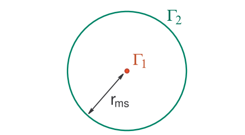
Figure 2: A configuration consisting of a uniformly charged spherical shell of charge $\Gamma_{2}$ surrounding a charge $\Gamma_{1}$ centered at the origin. $r_{\mathrm{ms}}$ is the coordinate BPS equilibrium distance.

The BPS solution of the field equations between two shells are identical to the usual spherical symmetric ones, with the appropriate enclosed charge substituted, and the solutions in adjacent regions matched by continuity. However, to get a complete (and stable) BPS configuration, the various energy contributions (energy stored in fields and “bare” mass of the shells) should precisely add up to $|Z(\Gamma)|_{r=\infty}$, with $\Gamma$ the total charge. Let us for example consider the one shell case of fig. 2. Denote the radius of the shell by $r_{\mathrm{ms}}$. The energy in the bulk fields outside the $\Gamma_{2}$-shell can be seen to be $E_{\mathrm{out}}=|Z(\Gamma)|_{r=\infty}-(e^{U}|Z(\Gamma)|)_{r=r_{\mathrm{ms}}}$, with $\Gamma=\Gamma_{1}+\Gamma_{2}$. The bare energy of the shell itself is $E_{\mathrm{shell}}=(e^{U}|Z(\Gamma_{2})|)_{r_{\mathrm{ms}}}$. The energy inside the shell is $E_{\mathrm{in}}=(e^{U}|Z(\Gamma_{2})|)_{r_{\mathrm{ms}}}$. So the total energy is

$$E_{\mathrm{tot}}=|Z(\Gamma)|_{\infty}+\left(e^{U}(|Z(\Gamma_{1})|+|Z(\Gamma_{2})|-|Z(\Gamma_{1})+Z(\Gamma_{2})|)\right)_{r_{\mathrm{ms}}}.$$ (17)

To saturate the BPS bound, the second term must vanish. This is the case if and only if the phases of $Z(\Gamma_{1})$ and $Z(\Gamma_{2})$ are equal for the values of the moduli at $r=r_{\mathrm{ms}}$, that is, if the flow in moduli space given by the solution crosses a surface of $(\Gamma_{1},\Gamma_{2})$ marginal stability at $r=r_{\mathrm{ms}}$ (explaining the subscript “ms” for this radius).

Because of the BPS condition, these configurations can be expected to be stable. To verify this, one can compute the force potential $W$ on a test particle of charge $\Gamma_{t}$ at rest in the background (BPS) field of a charge $\Gamma_{0}$, starting from the DBI+WZ action for a D-brane in an external field [17]. The result is:

$$W(r)=\left.2\,e^{U}\,|Z(\Gamma_{t})|\,\sin^{2}(\frac{\alpha_{t}-\alpha_{0}}{2})\,\,\right|_{r}\,,$$ (18)

where $\alpha_{i}=\arg Z(\Gamma_{i})$. This potential is everywhere positive, and acquires a zero minimum when $\alpha_{t}(r)=\alpha_{0}(r)$, that is, indeed, at marginal stability. A specific example is shown in fig. 3.

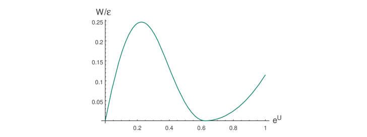
Figure 3: Example of a force potential for a test particle with charge $\epsilon\,\Gamma_{2}$ at rest in the background field of a BPS configuration like the one shown in fig. 2. As a convenient radial coordinate, we use the redshift factor $e^{U}$ (which increases monotonically from 0 to 1 when going from horizon to spatial infinity). For this particular example, we computed the potential numerically, using mirror symmetry and [30], for a type IIA compactification on the quintic, with, in the conventions of [5], $(Q_{D6},Q_{D4},Q_{D2},Q_{D0})(\Gamma_{1})=(1,2,5,-7)$, $(Q_{D6},Q_{D4},Q_{D2},Q_{D0})(\Gamma_{2})=(-1,1,4,-1)$, and vacuum modulus $\psi=7e^{i\pi/5}$.

4.2.2 Closed expression for equilibrium distance, and existence of solutions

A closed expression for the equilibrium radius $r_{\mathrm{ms}}$ can be extracted from the integrated flow equation (12) for the fields outside the shell. Taking the intersection product of $\Gamma_{1}$ with this equation gives, denoting $Z(\Gamma_{i})$ in short as $Z_{i}$:

$$2\mathop{\rm Im}\nolimits(e^{-U}e^{-i\alpha}Z_{1})=-\langle\Gamma_{1},\Gamma\rangle\,\tau+2\,\mathop{\rm Im}\nolimits(e^{-i\alpha}Z_{1})_{\tau=0}\,.$$ (19)

At $1/\tau=r=r_{\mathrm{ms}}$, the left-hand side is zero, so

$$r_{\mathrm{ms}}=\frac{\langle\Gamma_{1},\Gamma\rangle}{2\,\mathop{\rm Im}\nolimits(e^{-i\alpha}Z_{1})_{r=\infty}}\,.$$ (20)

Using $e^{i\alpha}=Z/|Z|$ with $Z=Z_{1}+Z_{2}$ and $\langle\Gamma_{1},\Gamma\rangle=\langle\Gamma_{1},\Gamma_{2}\rangle$, this can be written more symmetrically as

$$r_{\mathrm{ms}}=\frac{1}{2}\langle\Gamma_{1},\Gamma_{2}\rangle\left.\frac{|Z_{1}+Z_{2}|}{\mathop{\rm Im}\nolimits(\bar{Z_{2}}Z_{1})}\right|_{r=\infty}.$$ (21)

Such composite configurations will not exist for all possible charge combinations ($\Gamma_{1},\Gamma_{2}$) in a given vacuum. For example, a necessary condition for existence is obviously $r_{\mathrm{ms}}>0$, with $r_{\mathrm{ms}}$ given by charge and vacuum data as in (21). This is not a sufficient condition however. For example, the flow could hit a zero before it reaches the surface of $(\Gamma_{1},\Gamma_{2})$ marginal stability. Or the unique point in the flow where the left-hand side of (19) is zero, could correspond to a point in moduli space where $Z_{1}$ and $Z_{2}$ have opposite instead of equal phases. Furthermore, of course, $\Gamma_{2}$ has to exist as a BPS state for the values of the moduli at $r_{ms}$, and so should the solution inside the shell.

4.3 General, multicenter, stationary case

The above spherical solutions, while interesting and suggestive, are still not at the same level as genuine black hole soliton solutions of supergravity, in the sense that we explicitly added a smeared out charge source with a nonvanishing bare mass contribution to the total energy. On the other hand, the expression (18) for the potential of a test particle suggests the existence of truly solitonic BPS solutions with only point charges, located at equilibrium distance ($r_{\mathrm{ms}}$ in fig. 2) from each other. Such solutions, in the limit of a large number of charges positively proportional to $\Gamma_{2}$, evenly distributed over a sphere at $r=r_{\mathrm{ms}}$ from a black hole center with charge $\Gamma_{1}$, can be expected to approach the spherically symmetric case away from $r=r_{\mathrm{ms}}$. Sufficiently close to the $\Gamma_{2}$ charges on the other hand, the solution can be expected to approach a pure $\Gamma_{2}$ black hole solution.

To address this problem quantitavely, we should look for solutions to the general multicenter BPS equations given by (14)–(16). Because of the remark in footnote 4, we expect the relevant solution to involve mutually nonlocal charges. The latter complicates the situation considerably, since such configurations will in general not be static, because the right hand side of (15) is nonvanishing and hence $\omega$ cannot be gauged away.

4.3.1 Properties of muticenter solutions with mutually nonlocal charges

Assuming we have a solution to those equations, let us see what properties we can deduce. A first observation is that there will be constraints on the positions of the charges. Indeed, acting with ${\bf d}\boldsymbol{*}$ on equation (15) gives

$$0=\langle\Delta H,H\rangle\,,$$ (22)

with $\Delta$ the (flat) laplacian on $\mathbb{R}^{3}$, so, using (16) and $\Delta\tau_{p}=-4\pi\delta^{3}({\bf x}-{\bf x}_{p})$, we find that for all $p=1,\dots,N$:

$$\sum_{q=1}^{N}\frac{\langle\Gamma_{p},\Gamma_{q}\rangle}{|{\bf x}_{p}-{\bf x}_{q}|}=2\,\mathop{\rm Im}\nolimits\left(e^{-i\alpha}Z(\Gamma_{p})\right)_{r=\infty}.$$ (23)

Note that the full moduli space of solutions to the constraints (23) will have a fairly complicated structure. However, in the particular case of one source with charge $\Gamma_{1}$ at ${\bf x}=0$ and $M$ sources with charges postively proportional to $\Gamma_{2}$ at positions ${\bf x}_{p}$, the constraints simplify to

$$|{\bf x}_{p}|=\frac{\langle\Gamma_{2},\Gamma_{1}\rangle}{2\,\mathop{\rm Im}\nolimits(e^{-i\alpha}Z(\Gamma_{2}))_{r=\infty}}\,,$$ (24)

which is, as expected, precisely the equilibrium distance $r_{\mathrm{ms}}$ found in the spherical shell picture, equation (21).

Incidentally, by summing equation (23) over all $p$, one gets $\mathop{\rm Im}\nolimits(e^{-i\alpha}Z(\Gamma))_{\infty}=0$, with $\Gamma=\sum_{p}\Gamma_{p}$. On the other hand, by taking the intersection product of (14) with any $\Gamma_{p}$, and using (23), one sees that in the limit ${\bf x}\to{\bf x}_{p}$, that is, $\tau_{p}\to\infty$ and $\tau_{q}\to 1/|{\bf x}_{p}-{\bf x}_{q}|$ for $q\neq 0$, one has $\mathop{\rm Im}\nolimits(e^{-i\alpha}Z(\Gamma_{p}))\to 0$. Therefore we have

$$\alpha_{|{\bf x}|=\infty}=\arg Z(\Gamma)_{\infty}\qquad\mbox{ and }\qquad\alpha_{{\bf x}={\bf x}_{p}}=\arg Z(\Gamma_{p})_{{\bf x}_{p}}\,.$$ (25)

As argued under (11), the opposite sign for $e^{i\alpha}$ is to be excluded, as it gives an unphysical and severely singular negative mass solution, corresponding to a flow in the “wrong direction” in moduli space [17].

Note that this also implies that very far from all charges, as well as very close (in terms of coordinate distance) to any one of them, the solution will approach the single center case. Thus, if the solution exists, we can expect its image in moduli space to look like a fattened, “split” flow, as sketched in fig. 4. We will come back to this point in much more detail in section 4.3.2.

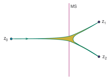
Figure 4: Sketch of the image of $z({\bf x})$ in moduli space for a multicenter solution containing two different charges $\Gamma_{1}$ and $\Gamma_{2}$, with attractor points $z_{1}$ resp. $z_{2}$, and modulus at spatial infinity $z_{0}$. The line labeled “MS” is a $(\Gamma_{1},\Gamma_{2})$-marginal stability line.

A second property that can be deduced directly from the equations is the total angular momentum of the solution. It is well known from ordinary Maxwell electrodynamics that multicenter configurations with mutually non-local charges (e.g. the monopole-electron system) can have intrinsic angular momentum even when the particles are at rest. The same turns out to be true here.

We define the angular momentum vector ${\bf J}$ from the asymptotic form of the metric (more precisely of $\omega$) as [31]

$$\omega_{i}=2\,\epsilon_{ijk}\,J^{j}\,\frac{x^{k}}{r^{3}}+O\left(\frac{1}{r^{3}}\right)\quad\mbox{for }r\longrightarrow\infty\,.$$ (26)

Plugging this expression in (15) and using (16) and (23), we find, after some work,

$${\bf J}=\frac{1}{2}\sum_{p<q}\langle\Gamma_{p},\Gamma_{q}\rangle\,{{\bf e}}_{pq}\,,$$ (27)

where ${{\bf e}}_{pq}$ is the unit vector pointing from ${\bf x}_{q}$ to ${\bf x}_{p}$:

$${{\bf e}}_{pq}=\frac{{\bf x}_{p}-{\bf x}_{q}}{|{\bf x}_{p}-{\bf x}_{q}|}\,.$$ (28)

Just like in ordinary electrodynamics, this is a “topological” quantity: it is invariant under continuous deformations of the solution, and quantized in half-integer units (more precisely, when all charges are on the z-axis, $2J_{z}\in\mathbb{Z}$). The appearance of intrinsic configurational angular momentum implies that quantization of these composites will have some non-trivial features. In particular, when many particles are involved, the ground state will presumably be highly degenerate.

4.3.2 Construction and existence of solutions

For simplicity, we will focus here on configurations with only two different kinds of charges $\Gamma_{1},\Gamma_{2}$, each distributed over $N$ centers $x_{1,a}$, resp. $x_{2,a}$, $a=1,\ldots,N$. We take $\Gamma_{1}$ and $\Gamma_{2}$ to be mutually nonlocal, $\langle\Gamma_{1},\Gamma_{2}\rangle\neq 0$. Centers of equal charge may coincide.

Then we can write the harmonic function $H$ of (16) as

$$H=-\Gamma_{1}\,V_{1}({\bf x})-\Gamma_{2}\,V_{2}({\bf x})\,\,+\,2\mathop{\rm Im}\nolimits\left(e^{-i\alpha}\Omega\right)_{r=\infty}\,,$$ (29)

with

$$V_{i}({\bf x})=\sum_{a=1}^{N}\frac{1}{|{\bf x}-{\bf x}_{i,a}|}\,,$$ (30)

and (23) becomes:

$$V_{12}\equiv V_{1}({\bf x}_{2,b})=V_{2}({\bf x}_{1,a})=\frac{2}{\langle\Gamma_{1},\Gamma_{2}\rangle}\left(\frac{\mathop{\rm Im}\nolimits(Z_{1}\bar{Z_{2}})}{|Z_{1}+Z_{2}|}\right)_{r=\infty}.$$ (31)

Taking the intersection product of (14) with the source charges $\Gamma_{1}$, $\Gamma_{2}$ and with a basis $\{\Gamma^{\perp}_{L}\}_{L}$ of the vector space spanned by the elements of $H^{3}(X,\mathbb{Z})$ which are local w.r.t. $\Gamma_{1},\Gamma_{2}$ (i.e., they have zero intersection with both $\Gamma_{1}$ and $\Gamma_{2}$), and using (31), we get the equations

$$2\,e^{-U}\mathop{\rm Im}\nolimits[e^{-i\alpha}Z_{1}] = -\langle\Gamma_{1},\Gamma_{2}\rangle\,(V_{2}({\bf x})-V_{12})\,,$$ (32)

$$2\,e^{-U}\mathop{\rm Im}\nolimits[e^{-i\alpha}Z_{2}] = -\langle\Gamma_{2},\Gamma_{1}\rangle\,(V_{1}({\bf x})-V_{12})\,,$$ (33)

$$2\,e^{-U}\mathop{\rm Im}\nolimits[e^{-i\alpha}Z^{\perp}_{L}] = 2\mathop{\rm Im}\nolimits[e^{-i\alpha}Z^{\perp}_{L}]_{r=\infty}\,(=\mbox{const.})\,.$$ (34)

This is a set of $2n+2$ independent equations, equivalent to (14), for $2n+2$ variables, where $n$ is the number of moduli.

Similarly, the second BPS equation (15) becomes

$$\boldsymbol{*}{\bf d}\,\omega = \langle\Gamma_{1},\Gamma_{2}\rangle[(V_{2}-V_{12}){\bf d}V_{1}-(V_{1}-V_{12}){\bf d}V_{2}]$$ (35)

$$= \langle\Gamma_{1},\Gamma_{2}\rangle\,(V_{1}-V_{12})(V_{2}-V_{12})\,{\bf d}\,\ln\left(\frac{V_{1}-V_{12}}{V_{2}-V_{12}}\right)\,.$$ (36)

We define two (local) space coordinate functions, $t$ and $\theta$, as follows:

$$V_{1}({\bf x})-V_{12}=t\cos\theta\quad;\quad V_{2}({\bf x})-V_{12}=t\sin\theta\,,$$ (37)

with $t>0$. So

$$t = \sqrt{(V_{1}-V_{12})^{2}+(V_{2}-V_{12})^{2}}\,,$$ (38)

$$\tan\theta = \frac{V_{1}-V_{12}}{V_{2}-V_{12}}\,.$$ (39)

To get a full (local) coordinate system, one of course has to choose a third coordinate function, but we leave this choice arbitrary here. Note that at spatial infinity, $t=V_{12}$ and $\theta=-3\pi/4$; at any of the $\Gamma_{1}$-charged centers, $t=\infty$ and $\theta=0$; and at any of the $\Gamma_{2}$-charged centers, $t=\infty$ and $\theta=\pi/2$. Generically, the range of $t$ on a surface of constant $\theta$ is finite and $\theta$-dependent. An example (with $N=1$) is shown in fig. 5.

We also introduce a $\theta$-dependent “effective charge” $\Gamma_{\theta}$:

$$\Gamma_{\theta}\equiv\cos\theta\,\Gamma_{1}+\sin\theta\,\Gamma_{2}\,.$$ (40)

Then we can rewrite equations (32)–(34) on a surface of fixed $\theta$ as:

$$2\,e^{-U}\mathop{\rm Im}\nolimits[e^{-i\alpha}Z_{1}] = -\langle\Gamma_{1},\Gamma_{\theta}\rangle\,t\,,$$ (41)

$$2\,e^{-U}\mathop{\rm Im}\nolimits[e^{-i\alpha}Z_{2}] = -\langle\Gamma_{2},\Gamma_{\theta}\rangle\,t\,,$$ (42)

$$2\,e^{-U}\mathop{\rm Im}\nolimits[e^{-i\alpha}Z^{\perp}_{L}] = 2\mathop{\rm Im}\nolimits[e^{-i\alpha}Z^{\perp}_{L}]_{r=\infty}\,(=\mbox{const.})\,,$$ (43)

or, going back to the compact form of the equations:

$$2\,\partial_{t}\left[e^{-U}\mathop{\rm Im}\nolimits(e^{-i\alpha}\Omega)\right]=-\Gamma_{\theta}.$$ (44)

This, together with the asymptotics of $\alpha$ at spatial infinity in (25), implies

$$\alpha=\arg Z(\Gamma_{\theta})\quad\mbox{or}\quad\alpha=\arg[-Z(\Gamma_{\theta})]\,.$$ (45)

Thus, comparing with (11), we see that if $\alpha=\arg Z(\Gamma_{\theta})$, (44) describes nothing but (part of) an ordinary single center flow for a charge $\Gamma_{\theta}$, while in the other case, $\alpha=\arg[-Z(\Gamma_{\theta})]$, it describes part of an inverted single center flow for a charge $\Gamma_{\theta}$. The only difference with (11) is the spatial parametrization of the flow. In the original case we had $\tau=1/r$ going from $0$ to $\infty$, here we have $t$ as in (38), which has a $\theta$-dependent range.

An important question is which of the two possibilities in (45) is satisfied at a given point ${\bf x}$. This is going to to be ${\bf x}$-dependent, since the asymptotic conditions (25) imply $\alpha=\arg[-Z_{\theta}]$ at spatial infinity, and $\alpha=\arg[Z_{\theta}]$ when approaching any of the centers. On the other hand, since $\alpha$ and $Z_{\theta}$ have to be continuous functions, the spatial surface on which the solution flips from one possibility to the other must have $Z_{\theta}=0$, that is, $Z_{2}/Z_{1}=-\tan\theta\in\mathbb{R}$; in other words, the moduli are at $(\Gamma_{1},\Gamma_{2})$- or at $(\Gamma_{1},-\Gamma_{2})$-marginal stability, for $\tan\theta\leq 0$ resp. $\tan\theta\geq 0$. The converse statement is also true, provided $t\neq 0$: if the moduli are at $(\Gamma_{1},\pm\Gamma_{2})$-marginal stability at a certain point ${\bf x}$ and $t\neq 0$, then $Z_{\theta}=0$. This follows directly from equations (42)–(43).

Because a surface of marginal stability has real codimension one in moduli space, and because of the asymptotics of (25), a surface of $(\Gamma_{1},\pm\Gamma_{2})$-marginal stability will in any case split the image of the solution in moduli space in two parts, as depicted in fig. 4: a region connected to the moduli at spatial infinity, where $alpha=\arg[-Z_{\theta}]$, and a region connected to the moduli at the centers, where $\alpha=\arg[Z_{\theta}]$. The corresponding regions in space are separated by a surface $\Sigma_{0}$ where $Z_{\theta}=0$ for some value of $\theta$. Furthermore, we can assume the marginal stability surface under consideration to be of $(\Gamma_{1},\Gamma_{2})$ type (so $\tan\theta\leq 0$ on $\Sigma_{0}$ if $t\neq 0$), as it is not possible to have only a $(\Gamma_{1},-\Gamma_{2})$-marginal stability surface intersecting the image in moduli space. This will become clear further on, but can be seen indirectly by imagining to vary continuously the moduli at spatial infinity to let them approach the intersecting surface of marginal stability; according to (31), the configuration will then degenerate to one with infinitely separated $\Gamma_{1}$- and $\Gamma_{2}$-centers, and the total mass will simply equal the sum of the BPS masses of the individual charges in the given vacuum. This total mass can only saturate the BPS bound if the marginal stability surface under consideration is of $(\Gamma_{1},\Gamma_{2})$-type.

Note that the solution will not necessarily exist: as noted under (11), complete inverted flows break down at a finite value of the flow parameter. Therefore, the $\Gamma_{\theta}$-flows for which $\alpha=\arg(-Z_{\theta})$ should have a range of $t$ that is not too large. We will study this problem in more detail below.

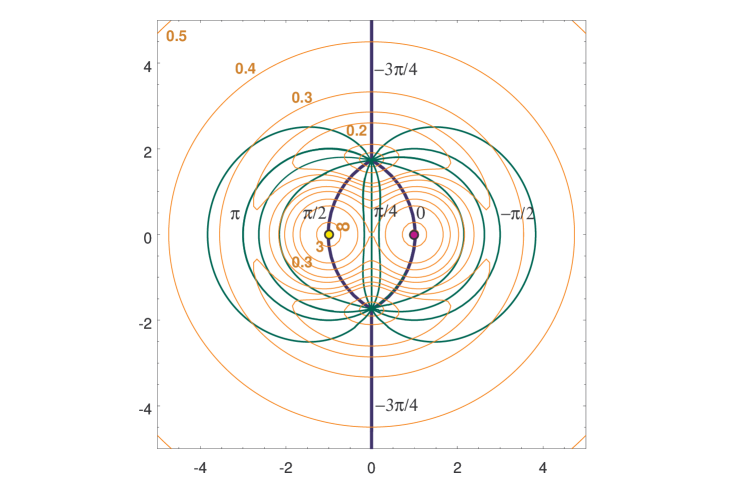
Figure 5: Surfaces of equal $t$ (thin orange lines) and equal $\theta$ (fatter green and even fatter blue lines) for a two center system with centers at ${\bf x}=(-1,0,0)$ and ${\bf x}=(1,0,0)$. Equal-$t$ surfaces with $t=0.2,0.3,0.4,0.5,3,\infty$ are indicated, as well as equal-$\theta$ surfaces with $\theta=0,\pi/4,\pi/2,\pi,-3\pi/4,-\pi/2$. The coordinate $t$ is minimal and equal to zero at the intersection locus of the equal-$\theta$ surfaces, and maximal (=$\infty$) at the positions of the centers. The fat blue lines ($\theta=0,\pi/2,-3\pi/4$) map to the skeleton split flow in moduli space.

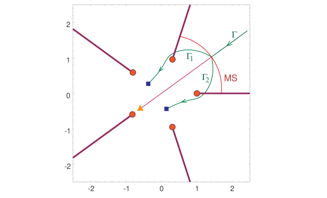
Figure 6: Numerically computed split flow for the example of fig. 3. A blue square indicates an attractor point with nonzero $|Z|$, an orange rectangle represents a regular zero. For graphical purposes, it is convenient to work in the $w$-plane, where $\arg w\equiv\arg\psi$ and $|w|=\frac{\ln(|\psi|+1)}{\ln 2}$. The horizontal and vertical axis indicates $\mathop{\rm Re}\nolimits w$ resp. $\mathop{\rm Im}\nolimits w$. The red dots are the five copies of the conifold point in this 5-fold cover of moduli space. MS is the $(\Gamma_{1},\Gamma_{2})$-marginal stability line. The purple line shows the continuation of the would-be $\Gamma_{1}+\Gamma_{2}$-flow beyond the split point.

To show how the partition in effective single center flows can be used to explicitly construct a (possibly numerical) solution, and thus to establish its existence, let us focus on the $N=1$ case shown in fig. 5. There exists a circle in space where $t=0$. From this locus, effective (generically partial, and possibly inverted) $\Gamma_{\theta}$-flows start for arbitrary values of $\theta$, together covering all of space. On the surface $\theta=-3\pi/4$, running to spatial infinity, the effective flow corresponds to an inverted flow with charge $\Gamma_{\theta}=-\frac{1}{\sqrt{2}}(\Gamma_{1}+\Gamma_{2})$, which image in moduli space is identical to that of a $\Gamma_{1}+\Gamma_{2}$-flow. When $\theta=0$, we have a pure, complete $\Gamma_{1}$-flow, and when $\theta=\pi/2$ a pure, complete $\Gamma_{2}$-flow. At $t=0$, the moduli must be at $(\Gamma_{1},\Gamma_{2})$-marginal stability, with $\alpha=\arg Z_{1}=\arg Z_{2}$ (this follows directly from (42)-(43) plus the asymptotic conditions (25)). Hence this point in moduli space is determined as the intersection of the $\Gamma_{1}+\Gamma_{2}$ flow starting from the moduli at spatial infinity with the surface of marginal stability. The $\theta=-3\pi/4$, $\theta=0$ and $\theta=\pi/2$ flows together form a “split flow”, as shown for a specific (numerically computed) quintic example in fig. 6. The (partial) flows for the other values of $\theta$ will fatten this split flow to something like fig. 7 (b). A subset of the flows with $\tan\theta<0$ will cross a zero of $Z_{\theta}$, namely where the surface of marginal stability is crossed in moduli space, as explained earlier and illustrated in fig. 7. Note that this does not lead to a breakdown of the solution, since at the same time, we jump from $\alpha=\arg(-Z_{\theta})$ to $\alpha=\arg Z_{\theta}$, such that the inverted $\Gamma_{\theta}$-flow we have up to the zero gets smoothly connected to an ordinary $\Gamma_{\theta}$-flow starting from the zero.

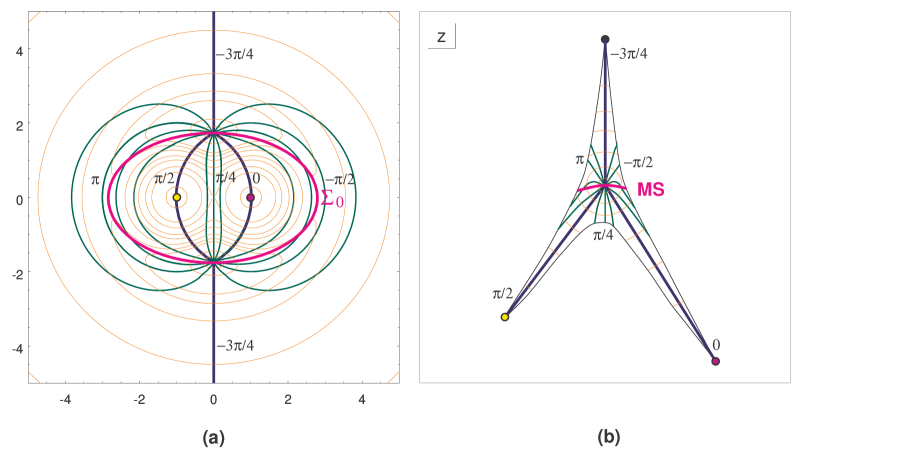
Figure 7: (a): Same as fig. 5, with additionally a possible location of the surface $\Sigma_{0}$ sketched (where the $(\Gamma_{1},\Gamma_{2})$-marginal stability line is crossed and the condition $\alpha=\arg(\pm Z_{\theta})$ flips). (b): Sketch of a possible corresponding image in moduli space, including the image of some lines of constant $\theta$ and $t$, and of $\Sigma_{0}$ (indicated as MS).

This construction shows that a multicenter solution for given center locations satisfying the constraint (31), will indeed exist, if each of the $\Gamma_{\theta}$ flows exists. The latter will be the case provided none of the $\Gamma_{\theta}$ flows crosses the $(\Gamma_{1},-\Gamma_{2})$-marginal stability surface (where $\tan\theta\geq 0$, $Z_{\theta}$ vanishes and the $\alpha=\arg(\pm Z_{\theta})$ condition flips), or, if some do, provided their $t$ range is not too large. It is quite plausible that this will be satisfied if and only if the “skeleton” split flow exists, though we will not try to prove this here. What could go wrong for example is that the partial $\Gamma_{\theta}$-flow for $\theta=\pi/4$, which finitely extends the incoming $\Gamma_{1}+\Gamma_{2}$-branch of the split flow, could hit a regular zero and have a maximal $t$ beyond the point where the inverted flow beyond the zero blows up. A necessary condition for this to happen is of course that the complete $\Gamma_{1}+\Gamma_{2}$-flow hits a regular zero. Such cases (as in the example of fig. 6) are quite interesting on their own, as they correspond to states that can only be realized as a multicenter solution; in particular they cannot be realized as a regular black hole.

Existence of the full multicenter solution will certainly be implied by existence of the skeleton split flow for many-center configurations approximating the idealized, uniformly charged spherical shell of fig. 2. Indeed, when we uniformly distribute an enormous number $N$ of $\Gamma_{2}$- centers on a sphere at equilibrium distance $r=r_{\mathrm{ms}}$ from a black hole center with charge $N\Gamma_{1}$, the corresponding fattened flow given by the multicenter solution will in fact be very thin, staying everywhere very close to the skeleton split flow. In the limit $N\to\infty$, the fattened flow becomes infinitely thin and reduces to the split flow itself. The $\Gamma_{1}+\Gamma_{2}$ branch corresponds to the solution outside the $\Gamma_{1}$ branch to the solution inside the shell, and the $\Gamma_{2}$ branch to the solution on (and near) the shell. This can be deduced directly from the above equations. It is plausible because away from the shell, in the limit $N\to\infty$ and on the scale of $r_{\mathrm{ms}}$, the situation reduces effectively to the idealized one depicted in fig. 2. On the other hand, when zooming in to the natural ${\bf x}$-coordinate scale close to the shell, one sees a number of $\Gamma_{2}$ centers, with separations of order $\sqrt{N}\to\infty$, floating around in a background with moduli value at $z^{a}_{\mathrm{ms}}$. Around each of those centers, we should therefore have a moduli flow corresponding to the $\Gamma_{2}$-branch of the split flow.

Actually, to get the full solution, we should also construct $\omega$ from (36). We did not do this explicitly, but because the position constraint (31) is in fact the integrability condition for this equation, a solution should certainly exist. In terms of $t$ and $\theta$, (36) reads, rather nicely:

$$\boldsymbol{*}d\,\omega=-\langle\Gamma_{1},\Gamma_{2}\rangle\,t^{2}\,d\theta\,.$$ (46)

Here $\boldsymbol{*}d\,\omega$ is actually the invariant local quantity (because $\omega$ can always be transformed to any $\omega+d\lambda$ by an ${\bf x}$-dependent time coordinate transformation), and hence of more physical significance than $\omega$ itself. Equation (46) is quite useful to visualize this quantity in specific configurations.

So our conclusion is: (at least some) regular multicenter BPS black hole solutions exist if and only if the corresponding split flow solution exists.

A final remark we want to make is that for multicenter BPS solutions involving also empty holes, this conclusion apparently does not hold: even when the split flow exist (with at least one branch, say $\theta=0$, ending on e.g. a conifold point) — and consequently also an idealized spherical shell solution — a corresponding multicenter solution (with point sources) does not seem to exist, because any $\Gamma_{\theta}$-flow with $\theta$ sufficiently small but nonzero, will hit a regular zero, and has at the same time an arbitrarily large maximal $t$, leading to a breakdown of the solution. This might be related to the delocalized nature of the source for empty holes, as discussed in section 4.1, but at this point, we do not have a concrete proposal for a resolution of this puzzle.

5 Composite configurations and existence of BPS states in string theory

5.1 A modified correspondence conjecture

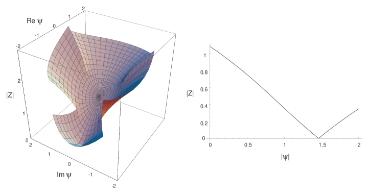
Figure 8: An example of a BPS state of type IIA string theory compactified on the quintic at the Gepner point, which does not have a corresponding single center black hole description. Left: modulus of the central charge as a function of the quintic modulus $\psi$ for the BPS state $|10000\rangle_{B}$ of [5] (with charge $(Q_{6},Q_{4},Q_{2},Q_{0})=(2,0,5,0)$), numerically computed using mirror symmetry. There is a regular zero at $\psi\approx-1.46$, hit by the flow starting at the Gepner point $\psi=0$. Right: $|Z|$ as a function of $|\psi|$ on the negative real axis.

As already mentioned in the introduction, it turns out that there are quite a few examples of BPS states known to exist in certain Calabi-Yau compactifications of type II string theory, which do not have a corresponding single center BPS black (or empty) hole solution, not even for large $N$. An example is given in fig. 8. Other examples are the higher dyons and the W-boson in Seiberg-Witten theory.

Strictly speaking, this disproves the correspondence conjecture of [16]. In [17], this puzzle and related paradoxes were studied in detail, and the necessity of considering more general stationary (multicenter) solutions in this context was demonstrated. Thus we are brought to the following adaptation of the correspondence conjecture, in its strongest form: a BPS state of a given charge exists in the full string theory if and only if a single or (possibly multi-) split attractor flow corresponding to that charge exists. Note that often, a BPS state can have several different realizations in the four dimensional low energy effective supergravity theory, either as an ordinary BPS black hole, corresponding to a single flow, or as one or more multicenter solutions (or spherical shell solutions), corresponding to one or more split flows. In fig. 9, it is shown how this modification of the conjecture indeed resolves the paradoxes as presented by the examples mentioned in the previous paragraph.

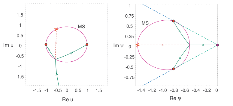
Figure 9: Numerically computed split flow for a $(2,-1)$-dyon at weak coupling in Seiberg-Witten theory (left) and for the state $|10000\rangle_{B}$ at the Gepner point $\psi=0$ of type IIA on the quintic (right). The former has $(\Gamma_{1},\Gamma_{2})=(2(1,-1),(0,1))$, the latter $(\Gamma_{1},\Gamma_{2})=((6,3,19,-10),(-4,-3,-14,10))$. The purple ellipsoid line is the relevant line of marginal stability, the dotted red line is the naive $(2,0,5,0)$ attractor flow, crashing on the regular zero of $Z$ indicated by a red cross. The wedge $4\pi/5<\arg\psi<6\pi/5$ is indicated by dashed lines. Both examples happen to involve empty hole charges only.

A much more detailed study of the BPS spectrum of the quintic from this effective field theory point of view will be presented in [21].

5.2 Marginal stability, Joyce transitions and $\Pi$-stability

From (21) or (23) or (31), it follows that when the moduli at infinity approach the the surface of $(\Gamma_{1},\Gamma_{2})$-marginal stability, the equilibrium distance between the $\Gamma_{1}$- and $\Gamma_{2}$-sources will diverge, eventually reaching infinity at marginal stability. Beyond the surface, the realization of this charge as a BPS $(\Gamma_{1},\Gamma_{2})$-composite no longer exists. This gives a nicely continuous four dimensional spacetime picture for the decay of the state when crossing a surface of marginal stability.

Furthermore, these formulae tell us at which side of the marginal stability surface the composite state can actually exist: since $r_{\mathrm{ms}}>0$, it is the side satisfying

$$\langle\Gamma_{1},\Gamma_{2}\rangle\,\sin(\alpha_{1}-\alpha_{2})>0\,,$$ (47)

where $\alpha_{i}=\arg Z(\Gamma_{i})_{r=\infty}$. Sufficiently close to marginal stability, this reduces to

$$\langle\Gamma_{1},\Gamma_{2}\rangle\,(\alpha_{1}-\alpha_{2})>0\,,$$ (48)

which is precisely the stability condition for “bound states” of special lagrangian 3-cycles found in a purely Calabi-Yau geometrical context by Joyce! (under more specific conditions, which we will not give here) [2, 14].

Note also that, since the right-hand side of (19) can only vanish for one value of $\tau$, the composite configurations we are considering here will actually satisfy

$$|\alpha_{1}-\alpha_{2}|<2\pi\,.$$ (49)

If the constituent $\Gamma_{i}$ of the composite configuration for which $\langle\Gamma,\Gamma_{i}\rangle>0$ can be identified with a “subobject” of the state as defined in [10], the above conditions imply that the phases satisfy the $\Pi$-stability criterion introduced in that reference. Though this similarity is interesting, it is not clear how far it extends. $\Pi$-stability seems to be considerably more subtle than what emerges here. It would be interesting to explore this connection further.

5.3 Non-BPS composites

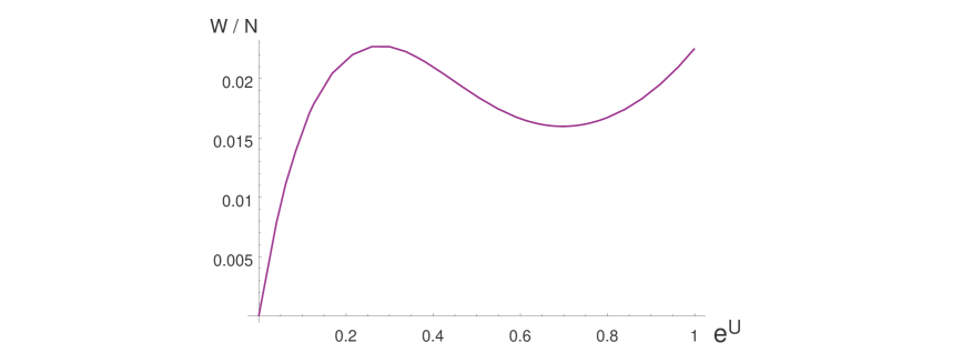
Figure 10: Potential $W$ (as a function of $e^{U}$) for a test particle of charge $(Q_{6},Q_{4},Q_{2},Q_{0})=(0,0,1,0)$ in the field of a charge $N(1,-1,-4,1)$ BPS black hole, for a quintic compactification at $w=10e^{\pi/5}$ (see fig. 6 for the definition of the modulus $w$). The nonzero minimum indicates the existence of a classically stable non-BPS configuration. In this case, a BPS black hole with the same total charge also exists, so the non-BPS state is possibly quantum mechanically unstable through tunneling.

From the discussion of section 4.2.1, one could also contemplate the existence of non-BPS composites. For example, what happens when we try to throw up to $N$ particles of charge $\Gamma_{2}$ into a black hole of charge $N\Gamma_{1}$, if we know that a composite BPS $(N\Gamma_{1},N\Gamma_{2})$-configuration does not exist? What does the ground state of this system look like in the low energy effective supergravity theory? One possibility is that a stable, statinary, non-BPS composite develops. Another possibility is that at a certain point, we simply cannot throw any $\Gamma_{1}$-particle into the black hole anymore, because it is repelled from it all the way up to spatial infinity. As a first approach to study non-BPS composites, one can look for nonzero minima of the force potential $W$ for a test particle in the field of a (BPS) black hole, equation (18). A configuration with this particle in its equilibrium position can then be expected to exist as a non-BPS solution.

A quintic example illustrating the possibility of having such a nonzero minimum is given in fig. 10.

6 Conclusions

We have proposed a modified version of the correspondence conjecture of [16] between BPS states in Calabi-Yau compactifications of type II string theory on the one hand, and four dimensional stationary ${\mathcal{N}}=2$ supergravity solutions on the other hand, and established a link between these solutions and split attractor flows in moduli space. Some interesting connections emerged, to the enhançon mechanism, the 3-pronged string picture of QFT BPS states, $\Pi$-stability and Joyce transitions of special lagrangian manifolds.

The most prominent open question is of course whether the conjecture (perhaps in a more refined form, as outlined in footnote 9) actually works. A more systematic comparison with known string theory results would be the obvious strategy for verifying this, but this is complicated considerably because of the fact that the number of cases that are accessible in both approaches at the same time, is rather limited. Some steps in that direction will be presented in [21].

Other interesting open question are: How to find a proper “multicenter” description of composite configurations involving empty holes? Is there a connection between D-brane moduli spaces and supergravity solution moduli spaces? Can those solution moduli spaces teach us something about the entropy of these states? What is the precise relation with $\Pi$-stability? Is there a link between the emergence of spatially extended configurations here and in the context of noncommutative brane effects, as for example in [32]? And who’s going to win the Subway Series, the Yankees or the Mets?

Hopefully some of these question will get an answer in the near future.