UT-913

hep-th/0010221

October, 2000

On Exact Noncommutative BPS Solitons

Masashi Hamanaka and Seiji Terashima

Department of Physics, University of Tokyo,
Tokyo 113-0033, Japan

Abstract

We construct new exact BPS solitons in various noncommutative gauge theories by the “gauge” transformation of known BPS solitons. This “gauge” transformation introduced by Harvey, Kraus and Larsen adds localized solitons to the known soliton. These solitons include, for example, the bound state of a noncommutative Abelian monopole and $N$ fluxons at threshold. This corresponds, in superstring theories, to a D-string which attaches to a D3-brane and $N$ D-strings which pierce the D3-brane, where all D-strings are parallel to each other.

1 Introduction

In the past few years, there has been much development in our understanding of various properties of noncommutative field theories. In particular, it has been shown that some noncommutative gauge theories can be embedded in string theories [1]-[3]. This fact means that there exist consistent noncommutative field theories even quantum mechanically and it is useful in understanding string theories to study noncommutative field theories.

In supersymmetric case, BPS solitons are important to investigate non-perturbative properties of noncommutative field theories as in string theories. Among them, instantons [4]-[14] and monopoles [15]-[28] in noncommutative gauge theories have been studied intensively. In string theories, the instanton and the monopole correspond to a D(p-4)-brane in a Dp-brane and a D(p-2)-brane attached to a Dp-brane, respectively.

On the other hand, some exact non-BPS solitons have been found in noncommutative field theories. They play an important role to study the condensation of the tachyon in non-BPS branes [29]-[49]. In particular, it was shown that a transformation of a solution of the equation of motion became a new solution of it and using this solution generating technique, the exact solitons were found in the effective open string field theory [48]. This transformation is almost a gauge transformation and is generated by a non-unitary operator $S$, which satisfies $S^{\dagger}S=1$ and $SS^{\dagger}=1-P$ where $P$ is a projection operator. This “gauge” transformation adds localized solitons to the known soliton. However, we easily see that the BPS equation is not always satisfied by the configuration constructed from the BPS soliton by this transformation. This is because the BPS equation has a constant part. For example, the transformation of $1+{\cal O}$ is $1+{\cal O}\rightarrow 1+S{\cal O}S^{\dagger}\neq S(1+{\cal O})S^{\dagger}$.

In this paper we construct new exact BPS solitons in some noncommutative gauge theories by the “gauge” transformation of known BPS solitons. This can be achieved by the tuning of parameters of theories or the modification of the transformation. Moreover, we add the constant elements to the transformed gauge fields which show the moduli parameters of the added localized solitons. These solitons include the bound state of a noncommutative Abelian monopole [23] and $N$ fluxons [25] at threshold. This corresponds, in superstring theories, to a D-string which attaches to a D3-brane and $N$ D-strings which pierce the D3-brane, where all D-strings are parallel to each other. The moduli parameters correspond to the positions of the $N$ fluxons.

This paper is organized as follows. In section 2, we briefly review the exact BPS solutions in noncommutative gauge theories. In section 3, we present a BPS-solution generating technique and construct new BPS solutions in noncommutative gauge theories. Finally section 4 is devoted to conclusion.

2 Review of some BPS Solutions

In this section, we shall review some BPS solutions in noncommutative gauge theories such as vortices [34, 41] and an Abelian monopole [23].

First we establish notations. The coordinates obey the following commutation relations

$$[x^{i},x^{j}]=i\theta^{ij}.$$ (2.1)

Here we consider the case for ${\rm rank}(\theta)=2$ and choose the convention of $\theta^{ij}$ as $\theta^{12}=\theta>0$. The case for ${\rm rank}(\theta)>2$ will be discussed later.

We introduce the complex coordinates as

$$z\equiv x^{1}+ix^{2},~{}~{}~{}\bar{z}\equiv x^{1}-ix^{2}.$$ (2.2)

Because of the space-space noncommutativity (2.1), we can define annihilation and creation operators in a Fock space ${\cal H}$ as

$$a\equiv\frac{1}{\sqrt{2\theta}}z,~{}~{}~{}a^{\dagger}\equiv\frac{1}{\sqrt{2\theta}}\bar{z},$$ (2.3)

so that

$$[a,a^{\dagger}]=1,~{}~{}~{}[a,a]=[a^{\dagger},a^{\dagger}]=0.$$ (2.4)

${\cal H}$ is spanned by $|n\rangle,{\rm where}~{}a^{\dagger}a|n\rangle=n|n\rangle,~{}n\geq 0$. Note that the derivative of an arbitrary operator $\phi$ with respect to the noncommutative coordinates $x^{i}$ can be written as $\partial_{i}\phi=[\hat{\partial}_{i},\phi]$ where $\hat{\partial}_{i}=-i(\theta^{-1})_{ij}x^{j}$.

Using anti-Hermitian operators

$$D_{i} \equiv \hat{\partial}_{i}+A_{i},$$ (2.5)

in the Fock space, we define the covariant derivatives as

$$\nabla_{i}\phi \equiv -\phi\,\hat{\partial}_{i}+D_{i}\phi,$$ (2.6)

$$\nabla_{i}\Phi \equiv [D_{i},\Phi],$$ (2.7)

where $\phi$ belongs to fundamental representation and $\Phi$ belongs to adjoint representation of the noncommutative gauge group. We can rewrite covariant operators $\nabla_{i}$ as

$$\nabla_{i}\phi=[\hat{\partial}_{i},\phi]+A_{i}\phi.$$ (2.8)

If we define

$$D_{z}=-\frac{1}{\sqrt{2\theta}}a^{\dagger}+A_{z}=\hat{\partial}_{z}+A_{z},\;\;\,\,D_{\bar{z}}=\frac{1}{\sqrt{2\theta}}a+A_{\bar{z}}=\hat{\partial}_{\bar{z}}+A_{\bar{z}}=-D_{z}^{\dagger},$$ (2.9)

these are also written by the complex coordinates as

$$\nabla_{z}\phi = -\phi\hat{\partial}_{z}+D_{z}\phi,\hskip 28.45274pt\nabla_{\bar{z}}\phi=-\phi\hat{\partial}_{\bar{z}}+D_{\bar{z}}\phi,$$ (2.10)

$$\nabla_{z}\Phi = [D_{z},\Phi],\hskip 14.22636pt\nabla_{\bar{z}}\Phi=[D_{\bar{z}},\Phi],$$ (2.11)

where $A_{z}\equiv\frac{1}{2}(A_{1}-iA_{2})$ and $A_{\bar{z}}=-A_{z}^{\dagger}\equiv\frac{1}{2}(A_{1}+iA_{2})$.

The field strength is given by

$$F_{ij}\equiv[D_{i},D_{j}]-i(\theta^{-1})_{ij},$$ (2.12)

and we also define the magnetic fields as $B_{i}\equiv-\displaystyle\frac{i}{2}\epsilon_{ijk}F^{jk}$ where $i,j,k=1,2,3$. Using the complex coordinates, we rewrite these as

$$F_{z\bar{z}} = -\left([D_{z},D_{z}^{\dagger}]+\frac{1}{2\theta}\right)$$ (2.13)

$$B_{z} \equiv \frac{1}{2}(B_{1}-iB_{2}),~{}~{}~{}B_{\bar{z}}\equiv\frac{1}{2}(B_{1}+iB_{2})$$ (2.14)

$$B_{3} = 2\left([D_{z},D_{z}^{\dagger}]+\frac{1}{2\theta}\right).$$ (2.15)

Note that $\int dx^{1}dx^{2}$ denotes $2\pi\theta{\rm Tr}$, where ${\rm Tr}$ is taken over ${\cal H}$.

Now we consider the BPS vortex solution in $(2+1)$-dimensional noncommutative Abelian Higgs model. The action of this gauge theory is given by

$$S=-\frac{1}{g^{2}_{\scriptsize\mbox{YM}}}\int dtd^{2}x~{}\left(-\frac{1}{4}F_{mn}F^{mn}+|\nabla_{m}\phi|^{2}+\frac{\beta}{2}(\phi\phi^{\dagger}-v^{2})^{2}\right),$$ (2.16)

where $\phi$ is a fundamental scalar field which is taken so that the coefficient of the kinetic term of $\phi$ should be $-1/g^{2}_{\scriptsize\mbox{YM}}$. Here we set the parameter $\beta=1$ so as to guarantee BPS condition [34]. The self-dual BPS equations are

$$B_{3}=v^{2}-\phi\phi^{\dagger},$$ (2.17)

$$\nabla_{\bar{z}}\phi=0,~{}~{}~{}\nabla_{z}\phi^{\dagger}=0.$$ (2.18)

The BPS solution for this theory have not been found for generic $\theta$. For the anti-self-dual BPS equations, however, at large $\theta$, the solution was derived in [34]. Note that this action and the BPS equations are not invariant under the permutation of $\phi$ and $\phi^{\dagger}$ because of the noncommutativity. This fact explains why the BPS states derived in [34] can not have the negative winding number. Similar argument holds in $(2+1)$-dimensional noncommutative pure Yang-Mills model [28].

In contrast to the Abelian Higgs model, exact BPS solutions in $(3+1)$-dimensional noncommutative Abelian gauge theory have been obtained in [23] [25]. Here we take $x^{0},~{}x^{3}$ as commutative coordinates and $x^{1},~{}x^{2}$ as noncommutative coordinates. The action is given by

$$S=-\frac{1}{4g^{2}_{\scriptsize\mbox{YM}}}\int d^{4}x~{}\left(F_{{\mu\nu}}F^{{\mu\nu}}+2\nabla_{\mu}\Phi\nabla_{\mu}\Phi\right),$$ (2.19)

where $\Phi$ is an adjoint Higgs field. The BPS equations are

$$B_{z}=\pm\nabla_{z}\Phi,~{}~{}~{}B_{\bar{z}}=\pm\nabla_{\bar{z}}\Phi,~{}~{}~{}B_{3}=\pm\nabla_{3}\Phi.$$ (2.20)

As is found in [23], the exact one-monopole solution of (2.20) is

$$\Phi = \sum_{n=0}^{\infty}\Phi_{n}|n\rangle\langle n|=\pm\left\{\sum_{n=1}^{\infty}\left(\xi_{n}^{2}-\xi_{n-1}^{2}\right)|n\rangle\langle n|+\left(\xi_{0}^{2}+\frac{x_{3}}{\theta}\right)|0\rangle\langle 0|\right\},$$

$$A_{z} = \frac{1}{\sqrt{2\theta}}\sum_{n=0}^{\infty}\left(1-\frac{\xi_{n}}{\xi_{n+1}}\right)a^{\dagger}|n\rangle\langle n|,~{}~{}~{}A_{3}=0,$$ (2.21)

where

$$\zeta_{n}\equiv\int_{0}^{\infty}dp~{}p^{n}e^{-\theta p^{2}+2px_{3}},~{}~{}~{}\xi_{n}\equiv\sqrt{\frac{n\zeta_{n-1}}{2\theta\zeta_{n}}}.$$ (2.22)

Here we understand $\xi_{0}=\sqrt{\frac{1}{2\theta\zeta_{0}}}$. The field strength of the solution is

$$B_{z} = \frac{1}{\sqrt{2\theta}}\sum_{n=0}^{\infty}\frac{\xi_{n}}{\xi_{n+1}}(\Phi_{n}-\Phi_{n+1})a^{\dagger}|n\rangle\langle n|,$$

$$B_{3} = \frac{1}{\theta}\sum_{n=1}^{\infty}\left(1-(n+1)\frac{\xi_{n}^{2}}{\xi_{n+1}^{2}}+n\frac{\xi_{n-1}^{2}}{\xi_{n}^{2}}\right)|n\rangle\langle n|+\frac{1}{\theta}\left(1-\frac{\xi_{0}^{2}}{\xi_{1}^{2}}\right)|0\rangle\langle 0|.$$ (2.23)

We note that the action (2.19) can be regarded as the effective action on the world volume of a D-brane. Indeed, it was shown that taking the zero slope limit [3], the tree-level world volume action of Dp-branes in background NS-NS $B$ field becomes the $(p+1)$-dimensional noncommutative gauge theory with sixteen supersymmetries. Here the noncommutativity is given by $\theta=1/B$. This theory has $9-p$ Higgs fields $\Phi^{\hat{\mu}}$ which correspond to the transverse coordinates. The action (2.19) is obtained from this world volume action by setting $\Phi^{\hat{\mu}}=0$ where ${\hat{\mu}}=5,\ldots,9$ and $\Phi^{4}\equiv\Phi$. A monopole solution corresponding to a D(p-2)-brane is mapped to an anti-monopole solution corresponding to an anti-D(p-2)-brane by $\Phi\rightarrow-\Phi$.

3 BPS-Solution Generating Technique and New BPS Solutions

Now we will construct exact new BPS solutions by transformation of BPS solutions. The transformation generating operator $S$ is defined as

$$S^{\dagger}S=1,~{}~{}~{}SS^{\dagger}=1-P_{1},$$ (3.1)

where $P_{N}$ is a projection operator onto $N$-dimensional subspace of ${\cal H}$ and defined as

$$P_{N}\equiv\sum_{m=0}^{N-1}|m\rangle\langle m|.$$ (3.2)

The almost unitary generator $S$ and the projection $P_{1}$ satisfy the equations

$$P_{1}S=S^{\dagger}P_{1}=0.$$ (3.3)

Up to the noncommutative gauge equivalence, this operator is represented in the occupation number basis as

$$S = \sum_{n=0}^{\infty}|n+1\rangle\langle n|,~{}~{}~{}S^{\dagger}=\sum_{n=0}^{\infty}|n\rangle\langle n+1|.$$ (3.4)

We also define the following operator

$$S_{N} \equiv S^{N}=\sum_{n=0}^{\infty}|n+N\rangle\langle n|,~{}~{}~{}S_{N}^{\dagger}\equiv(S^{\dagger})^{N}=\sum_{n=0}^{\infty}|n\rangle\langle n+N|,$$ (3.5)

which satisfies

$$S_{N}^{\dagger}S_{N}=1,~{}~{}~{}S_{N}S_{N}^{\dagger}=1-P_{N},~{}~{}~{}P_{N}S_{N}=S_{N}^{\dagger}P_{N}=0.$$ (3.6)

We shall transform the gauge field $A$ (or anti-Hermitian operator $D=d+A$) and the Higgs fields $\phi$ and $\Phi$ by the transformation generating operator $S,S^{\dagger}$ as

$$D_{z}\rightarrow S_{N}D_{z}S_{N}^{\dagger},\,\,\,\,\,\Phi\rightarrow S_{N}\Phi S_{N}^{\dagger},\,\,\,\,\,\phi\rightarrow S_{N}\phi.$$ (3.7)

This transformation is similar to the noncommutative gauge transformation. From now on, we will call this transformation “gauge” transformation. Note that the solution of the equation of motion is transformed by $S_{N}$ to another solution of the equation of motion as was discussed in [48]. (see also [9] [11] [13] [32] [46].)

In the following, we will construct a set of new solutions of the BPS equations, instead of the solution of the equations of motion, by this “gauge” transformation from BPS solutions. Moreover, we will find that the transformed gauge fields can have the constant elements which show moduli parameters.

3.1 New Exact BPS Solution in $(2+1)$-dimensional Noncommutative Abelian Higgs Model

Suppose that a set of gauge field $A$ and Higgs field $\phi$ is BPS solution in $(2+1)$-dimensional noncommutative Abelian Higgs model with the action (2.16), i.e. it satisfies BPS equations (2.17), (2.18). First, let us transform it by the “gauge” transformation (3.7). Under this transformation, the left and right hand side of the BPS equations (2.17), (2.18) becomes

l.h.s. of (2.17) $$: B_{3}=2[D_{z},D_{z}^{\dagger}]+\frac{1}{\theta}\rightarrow S_{N}\left(2[D_{z},D_{z}^{\dagger}]+\frac{1}{\theta}\right)S_{N}^{\dagger}+\frac{1}{\theta}P_{N}$$ (3.8)

r.h.s. of (2.17) $$: v^{2}-\phi\phi^{\dagger}\rightarrow S_{N}(v^{2}-\phi\phi^{\dagger})S_{N}^{\dagger}+v^{2}P_{N},$$ (3.9)

l.h.s. of (2.18) $$: \nabla_{\bar{z}}\phi\rightarrow S_{N}\nabla_{\bar{z}}\phi,~{}~{}~{}\nabla_{z}\phi^{\dagger}\rightarrow(\nabla_{z}\phi^{\dagger})S_{N}^{\dagger}.$$ (3.10)

From the above relations, we can find a new BPS solution by the “gauge” transformation of an original BPS solution only for $\theta=1/v^{2}$ , which means that the scale of noncommutativity equals to that of vortices. Here we note that BPS equations still remain intact adding the elements $\sum_{m=0}^{N-1}\lambda_{m}|m\rangle\langle m|$, where $\lambda_{m}$ are constants, to the transformed gauge fields. General solution is

$$D_{z}^{\scriptsize\mbox{new}}=S_{N}D_{z}S_{N}^{\dagger}+\sum_{m=0}^{N-1}\lambda^{z}_{m}|m\rangle\langle m|,~{}~{}~{}\phi^{\scriptsize\mbox{new}}=S_{N}\phi,$$ (3.11)

where $\lambda^{z}_{m}$ are arbitrary complex constants and are interpreted as the positions of the solitons added by the transformation [28].

The solution constructed from the vacuum state $A_{z}=0,~{}\phi=v$ is the solution found by Bak [41] setting all $\lambda^{z}_{m}$ zero:

$$\phi=v\sum_{n=0}^{\infty}|n+N\rangle\langle n|,~{}~{}~{}A_{z}=-\frac{1}{\sqrt{2\theta}}\sum_{n=0}^{\infty}\left(1-\sqrt{\frac{n+1-N}{n+1}}\right)a^{\dagger}|n\rangle\langle n|.$$ (3.12)

As long as $\theta=1/v^{2}$, we can construct various BPS solution $D_{z}^{\scriptsize\mbox{new}}$ and $\phi^{\scriptsize\mbox{new}}$ from arbitrary known BPS solutions besides the vacuum.

3.2 New Exact BPS Solution in $(3+1)$-dimensional Noncommutative Abelian Gauge Theory

Next, we consider $(3+1)$-dimensional noncommutative Abelian gauge theory with an adjoint Higgs field. The action is given by (2.19). Suppose that a set of gauge fields $A_{i}$ and adjoint Higgs field $\Phi$ is BPS solution, i.e. it satisfies BPS equations

$$2[D_{z},D_{z}^{\dagger}]+\frac{1}{\theta} = \pm[D_{3},\Phi],$$ (3.13)

$$[D_{3},D_{z}] = \pm[D_{z},\Phi].$$ (3.14)

Let’s transform the gauge fields $A_{i}$ and adjoint Higgs field $\Phi$ as

$$D_{z}\rightarrow S_{N}D_{z}S_{N}^{\dagger},~{}~{}~{}\Phi\rightarrow S_{N}\Phi S_{N}^{\dagger},$$ (3.15)

$$D_{3}=\partial_{3}+A_{3}\rightarrow\partial_{3}+S_{N}A_{3}S_{N}^{\dagger}.$$

Note that we do not transform $D_{3}$ as $D_{3}\rightarrow S_{N}D_{3}S_{N}^{\dagger}$. $S_{N}$ does not depend on $x^{3}$ and satisfies $S_{N}^{\dagger}S_{N}=1,~{}S_{N}S_{N}^{\dagger}=1-P_{N}$. Under this “gauge” transformation, the left and right hand side of the BPS equation becomes

l.h.s. of (3.13) $$: 2[D_{z},D_{z}^{\dagger}]+\frac{1}{\theta}\rightarrow S_{N}\left(2[D_{z},D_{z}^{\dagger}]+\frac{1}{\theta}\right)S_{N}^{\dagger}+\frac{1}{\theta}P_{N},$$ (3.16)

r.h.s. of (3.13) $$: [D_{3},\Phi]\rightarrow S_{N}[D_{3},\Phi]S_{N}^{\dagger},$$ (3.17)

l.h.s. of (3.14) $$: [D_{3},D_{z}]\rightarrow S_{N}[D_{3},D_{z}]S_{N}^{\dagger},$$ (3.18)

r.h.s. of (3.14) $$: [D_{z},\Phi]\rightarrow S_{N}[D_{z},\Phi]S_{N}^{\dagger},$$ (3.19)

From the above relation, we should modify the “gauge” transformation for $\Phi$, so that the transformed configuration should be BPS. The modified “gauge” transformation would be

$$\Phi \rightarrow S_{N}\Phi S_{N}^{\dagger}\pm\frac{x^{3}}{\theta}P_{N}.$$ (3.20)

This transformation leaves the BPS equations (3.13), (3.14) intact because the transformation of r.h.s. of (3.13) is modified as $[D_{3},\Phi]\rightarrow S_{N}[D_{3},\Phi]S_{N}^{\dagger}\pm\frac{1}{\theta}P_{N}$ and that of r.h.s. of (3.13) is the same as (3.19) owing to $S_{N}^{\dagger}P_{N}=P_{N}S_{N}=0$. Moreover, as in the case of vortices, BPS equations still remain intact adding the constant elements to the transformed gauge fields. General solution is

$$\Phi^{\scriptsize\mbox{new}} = S_{N}\Phi S_{N}^{\dagger}\pm\frac{x^{3}}{\theta}P_{N}+\sum_{m=0}^{N-1}\lambda^{4}_{m}|m\rangle\langle m|,$$ (3.21)

$$D_{3}^{\scriptsize\mbox{new}} = \partial_{3}+S_{N}A_{3}S_{N}^{\dagger}+\sum_{m=0}^{N-1}\lambda^{3}_{m}|m\rangle\langle m|,$$ (3.22)

$$D_{z}^{\scriptsize\mbox{new}} = S_{N}D_{z}S_{N}^{\dagger}+\sum_{m=0}^{N-1}\lambda^{z}_{m}|m\rangle\langle m|.$$ (3.23)

where $\lambda_{m}^{z}\equiv\lambda_{m}^{1}+i\lambda_{m}^{2}$ and $\lambda_{m}^{1},~{}\lambda_{m}^{2},~{}\lambda_{m}^{3},~{}\lambda_{m}^{4}$ are arbitrary real constants.

The solution constructed from the vacuum state $A=0,~{}\Phi=0$ is the $N$-fluxon solution [25]

$$D_{z} = S_{N}\hat{\partial}_{z}S_{N}^{\dagger},~{}~{}~{}A_{3}=0,~{}~{}~{}\Phi=\pm\frac{x^{3}}{\theta}P_{N}.$$ (3.24)

In [23], an exact BPS solution (2) have been constructed in noncommutative Abelian gauge theory by Nahm construction. They also found the solution (3.24) that describes infinite D1 strings piercing a D3 brane, which they call the fluxons [25]. Here we construct a new solution by the “gauge” transformation from the solutions (2). The solution is following

$$\Phi^{\scriptsize\mbox{new}} = =\sum_{n=N}^{\infty}\Phi_{n-N}|n\rangle\langle n|+\sum_{m=0}^{N-1}\left(\pm\frac{x^{3}}{\theta}+\lambda^{4}_{m}\right)|m\rangle\langle m|,$$

$$D_{z}^{\scriptsize\mbox{new}} = =\frac{1}{\sqrt{2\theta}}\sum_{n=N}^{\infty}\sqrt{\frac{n+1-N}{n+1}}\frac{\xi_{n-N}}{\xi_{n+1-N}}a^{\dagger}|n\rangle\langle n|+\sum_{m=0}^{N-1}\lambda^{z}_{m}|m\rangle\langle m|,$$

$$A_{3}^{\scriptsize\mbox{new}} = \sum_{m=0}^{N-1}\lambda_{m}^{3}|m\rangle\langle m|.$$ (3.25)

This solution can be interpreted as the bound state at threshold of an Abelian monopole and $N$ fluxons (Figure 1).

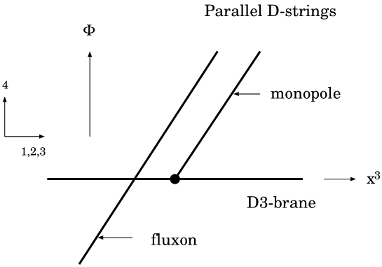
Figure 1: Bound state at threshold of an Abelian monopole and $N$ fluxons ($N$=1)

The new solution can be represented as

$$D^{\scriptsize\mbox{new}}=S_{N}DS_{N}^{\dagger}+\sum_{m=0}^{N-1}\lambda_{m}|m\rangle\langle m|=\left(\begin{array}[]{ccc|c}\lambda_{0}&{}\hfil&O&{}\hfil\\ {}\hfil&\ddots&{}\hfil&O\\ O&{}\hfil&\lambda_{N-1}&{}\hfil\\ \hline\cr{}\hfil&O&{}\hfil&D\end{array}\right),$$ (3.30)

where $\lambda_{m}$ are real constants. The transformation by $S_{N}$ corresponds to the shift of the matrix elements in the lower-right direction by $N$ [46]. The $\lambda_{m}$ can be interpreted as the coordinates of localized solitons in matrix theoretical picture although the action is difficult to be realized in the matrix models [50]-[52] because of the commutative coordinates $x^{0}$ and $x^{3}$. In this monopole case, the localized solitons are fluxons. This picture is also applicable to vortices and instantons.

We have set the transverse coordinates $\Phi^{\hat{\mu}}=0$ in the last paragraph in section 2. After the transformation, however, we can take $\Phi^{\hat{\mu}}\neq 0$ keeping the BPS condition. For example, to the general solutions (3.21)-(3.23), we can set

$$\Phi^{\hat{\mu}}=\sum_{m=0}^{N-1}\lambda_{m}^{\hat{\mu}}|m\rangle\langle m|=\left(\begin{array}[]{ccc|c}\lambda_{0}^{\hat{\mu}}&{}\hfil&O&{}\hfil\\ {}\hfil&\ddots&{}\hfil&O\\ O&{}\hfil&\lambda_{N-1}^{\hat{\mu}}&{}\hfil\\ \hline\cr{}\hfil&O&{}\hfil&O\end{array}\right),$$ (3.35)

where $\lambda_{m}^{\hat{\mu}},~{}{\hat{\mu}}=5,\ldots,9$ are real constants and denote the ${\hat{\mu}}$-th transverse coordinates of the $m$-th fluxon. This shows that the $N$ fluxons can escape from the D3-brane (Figure 2).

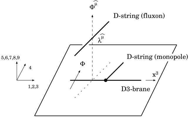
Figure 2: Fluxons can escape from the D3-brane.

3.3 Exact BPS Instanton Solution in $4$-dimensional Noncommutative Gauge Theory

As in the previous case, we can also obtain the exact BPS solutions in $4$-dimensional Euclidean noncommutative gauge theory with the action

$$S=-\frac{1}{4g^{2}_{\scriptsize\mbox{YM}}}\int d^{4}x~{}{\rm Tr}\,F_{{\mu\nu}}F^{{\mu\nu}}.$$ (3.36)

The BPS equations are

$$F_{z_{1}\bar{z}_{1}}\pm F_{z_{2}\bar{z}_{2}}=0,~{}~{}~{}F_{z_{1}z_{2}}=0,$$ (3.37)

where $z_{1}\equiv x^{1}+ix^{2},~{}z_{2}\equiv x^{3}+ix^{4}$.

Here we restrict ourselves to consider the gauge theory with the anti-self-dual noncommutative parameter $\theta^{{\mu\nu}}$. In this case, we can take $\theta^{12}=\theta>0,\theta^{34}=-\theta$ and (other components) $=0$ without loss of generality. We define anti-Hermitian operators as

$$D_{z_{i}} \equiv -\frac{1}{2\theta}\bar{z}_{i}+A_{z_{i}},$$ (3.38)

where $i=1,2$ and $A_{z_{1}}\equiv\frac{1}{2}(A_{1}-iA_{2}),~{}A_{z_{2}}\equiv\frac{1}{2}(A_{3}-iA_{4})$.

For the anti-self-dual $\theta$, the self-dual noncommutative instantons were investigated intensively. In particular, their moduli space is resolved by noncommutativity. Thus the instanton can not escape from the brane and we can construct the instanton even in the commutative $U(1)$ gauge theory with DBI action [3] [6]. However, the anti-self-dual noncommutative instanton has the same moduli space as commutative one which has small instanton singularities. The solution which can be obtained by the “gauge” transformation is an anti-self-dual BPS solution [46] since the added solitons can escape from the brane. Thus we concentrate on the anti-self-dual BPS solution.

Suppose that $A_{\mu}$ is an anti-self-dual BPS solution in 4-dimensional noncommutative gauge theory, i.e. it satisfies the anti-self-dual BPS equation

$$[D_{z_{1}},D^{\dagger}_{z_{1}}]+[D_{z_{2}},D^{\dagger}_{z_{2}}]=0,~{}~{}~{}[D_{z_{1}},D_{z_{2}}]=0.$$ (3.39)

We note that the constants terms in

$$F_{z_{i}\bar{z}_{i}}=-[D_{z_{i}},D_{z_{i}}^{\dagger}]+\frac{1}{2\theta}(-1)^{i},$$ (3.40)

are canceled in the anti-self-dual BPS equation (3.39).

In this instanton case, the state of the Fock space ${\cal H}_{1}\otimes{\cal H}_{2}$ is labeled by two non-negative integer numbers e.g. $|n_{1},n_{2}\rangle$. Hence we shall introduce a transformation generating operator $T$ [46] as

$$T^{\dagger}T=1,~{}~{}~{}TT^{\dagger}=1-P,$$ (3.41)

where $P$ is a projection operator in the Fock space ${\cal H}_{1}\otimes{\cal H}_{2}$ which project onto the finite dimensional subspace of ${\cal H}_{1}\otimes{\cal H}_{2}$. We can show $PT=(1-TT^{\dagger})T=0$. Using this almost unitary operator $T$, we shall transform $D$ as before

$$D_{z_{i}}\rightarrow TD_{z_{i}}T^{\dagger}.$$ (3.42)

Since

$$[D_{z_{i}},D_{z_{j}}] \rightarrow T[D_{z_{i}},D_{z_{j}}]T^{\dagger},$$ (3.43)

$${[D_{z_{i}},D^{\dagger}_{z_{j}}]} \rightarrow T[D_{z_{i}},D^{\dagger}_{z_{j}}]T^{\dagger},$$ (3.44)

we can construct a new BPS solution from the original BPS solution by the transformation (3.42). As in the previous case, we introduce a projection $P_{m}$ onto the single state which satisfies ${\rm Tr}P_{m}=1$ and $P=\sum_{m=0}^{N-1}P_{m}$. Then general solution constructed by this way can be written as

$$D_{z_{i}}^{\scriptsize\mbox{new}}=TD_{z_{i}}T^{\dagger}+\sum_{m=0}^{N-1}\lambda^{i}_{m}P_{m},$$ (3.45)

where $i=1,2$ and $\lambda^{i}_{m}$ are arbitrary complex constants. As in the monopole case, we can also set $\Phi^{\hat{\mu}}$ as (3.35). The localized solitons are identified as small instantons. This shows that the $N$ small instantons which correspond to $N$ D(p-4)-branes can escape from the Dp-brane.

The solution (3.45) constructed from the vacuum state $A=0$ was derived in [46]. As long as the self-duality of the gauge fields is the same as that of noncommutative parameters $\theta^{{\mu\nu}}$, we can construct various BPS solution from arbitrary known BPS solutions besides the vacuum, e.g. from $U(2)$ 1-instanton solution in [14]. We can see that the BPS solution constructed from the BPS solution with the instanton number $M$ has the instanton number $M+N$ where $N={{\rm Tr}\,}P$ because of the properties of the projection.

4 Conclusion

In this paper, we have constructed exact BPS solitons in various noncommutative gauge theories by the “gauge” transformation of known BPS solitons. These solutions have appropriate physical interpretations, for example, we have found the bound state of a noncommutative Abelian monopole and $N$ fluxons at threshold. This corresponds, in superstring theories, to a D-string which attaches to a D3-brane and $N$ D-strings which pierce the D3-brane, where all D-strings are parallel to each other.

If we treat non-Abelian gauge theories, we should add Chan-Paton index $i$ to the state, i.e. the state is written as $|n,i\rangle$ . Then it is trivial to extend the solution generating technique to the non-Abelian gauge theory and we can use the $U(2)$ monopole solution [28] and $U(2)$ anti-self-dual instanton solution [14]. The BPS solution for a non-Abelian Higgs model can be also obtained from the vacuum.

The application for another noncommutative BPS solitons remains to be investigated. In ${\bf C}P_{n}$ model on noncommutative plane [53], it seems to be difficult to generate another BPS solution from a BPS solution except for the solution from the vacuum. It is interesting to study which noncommutative theories our technique would be to apply to.

Acknowledgements

We would like to thank Y. Matsuo for useful comments and encouragement. We are also grateful to K. Furuuchi, K. Hosomichi, T. Kawano, T. Takayanagi and T. Uesugi for discussion. The work of S.T. was supported in part by JSPS Research Fellowships for Young Scientists. The work of M.H. was supported in part by the Japan Securities Scholarship Foundation (#12-3-0403).

Note Added

After submitting this paper, we received the paper [54] which partially overlaps our results.

References

• [1] A. Connes, M. R. Douglas and A. Schwarz, JHEP 9802 (1998) 003, hep-th/9711162
• [2] M. R. Douglas and C. Hull, JHEP 9802 (1998) 008, hep-th/9711165
• [3] N. Seiberg and E. Witten, JHEP 9909 (1999) 032, hep-th/9908142
• [4] N. Nekrasov and A. Schwarz, Comm. Math. Phys. 198 (1998) 689-703, hep-th/9802068
• [5] M. Marino, R. Minasian, G. Moore and A. Strominger, JHEP 0001 (2000) 005, hep-th/9911206
• [6] S. Terashima, Phys. Lett. B477 (2000) 292, hep-th/9911245
• [7] H. W. Braden and N. A. Nekrasov, “Space-time foam from non-commutative instantons,” hep-th/9912019
• [8] K. Furuuchi, Prog. Theor. Phys. 103 (2000) 1043, hep-th/9912047
• [9] P. Ho, “Twisted bundle on noncommutative space and U(1) instanton,” hep-th/0003012
• [10] K. Kim, B. Lee and H. S. Yang, “Comments on instantons on noncommutative ${\bf R}^{4}$,” hep-th/0003093
• [11] K. Furuuchi, “Equivalence of projections as gauge equivalence on noncommutative space,” hep-th/0005199
• [12] K. Lee, D. Tong and S. Yi, “The moduli space of two U(1) instantons on noncommutative ${\bf R}^{4}$ and ${\bf R}^{3}\times S^{1}$,” hep-th/0008092
• [13] N. A. Nekrasov, “Noncommutative instantons revisited,” hep-th/0010017
• [14] K. Furuuchi, “Dp-D(p+4) in Noncommutative Yang-Mills” hep-th/0010119
• [15] A. Hashimoto and K. Hashimoto, JHEP 9911 (1999) 005, hep-th/9909202
• [16] D. Bak, Phys. Lett.  B471 (1999) 149, hep-th/9910135
• [17] K. Hashimoto, H. Hata and S. Moriyama, JHEP 9912 (1999) 021, hep-th/9910196
• [18] L. Jiang, “Dirac monopole in non-commutative space,” hep-th/0001073
• [19] D. Mateos, Nucl. Phys.  B577 (2000) 139, hep-th/0002020
• [20] K. Hashimoto and T. Hirayama, “Branes and BPS configurations of noncommutative / commutative gauge theories,” hep-th/0002090
• [21] S. Moriyama, Phys. Lett.  B485 (2000) 278, hep-th/0003231
• [22] S. Goto and H. Hata, Phys. Rev.  D62 (2000) 085022, hep-th/0005101
• [23] D. J. Gross and N. A. Nekrasov, JHEP 0007 (2000) 03, hep-th/0005204
• [24] S. Moriyama, JHEP 0008 (2000) 014, hep-th/0006056
• [25] D. J. Gross and N. A. Nekrasov, “Dynamics of strings in noncommutative gauge theory,” hep-th/0007204
• [26] J. G. Russo and M. M. Sheikh-Jabbari, “Strong coupling effects in non-commutative spaces from OM theory and supergravity,” hep-th/0009141
• [27] K. Hashimoto, T. Hirayama and S. Moriyama, “Symmetry origin of nonlinear monopole,” hep-th/0010026
• [28] D. J. Gross and N. A. Nekrasov, “Solitons in noncommutative gauge theory,” hep-th/0010090
• [29] R. Gopakumar, S. Minwalla and A. Strominger, JHEP 0005 (2000) 020, hep-th/0003160
• [30] K. Dasgupta, S. Mukhi and G. Rajesh, JHEP 0006 (2000) 022, hep-th/0005006
• [31] J. A. Harvey, P. Kraus, F. Larsen and E. J. Martinec, JHEP 0007 (2000) 042, hep-th/0005031
• [32] E. Witten, “Noncommutative tachyons and string field theory,” hep-th/0006071
• [33] A. P. Polychronakos, “Flux tube solutions in noncommutative gauge theories,” hep-th/0007043
• [34] D. P. Jatkar, G. Mandal and S. R. Wadia, JHEP 0009 (2000) 018, hep-th/0007078
• [35] D. Bak and K. Lee, “Elongation of moving noncommutative solitons,” hep-th/0007107
• [36] R. Gopakumar, S. Minwalla and A. Strominger, “Symmetry restoration and tachyon condensation in open string theory,” hep-th/0007226
• [37] A. S. Gorsky, Y. M. Makeenko and K. G. Selivanov, “On noncommutative vacua and noncommutative solitons,” hep-th/0007247
• [38] C. Zhou, “Noncommutative scalar solitons at finite Theta,” hep-th/0007255
• [39] N. Seiberg, JHEP 0009 (2000) 003, hep-th/0008013
• [40] Y. Hikida, M. Nozaki and T. Takayanagi, “Tachyon condensation on fuzzy sphere and noncommutative solitons,” hep-th/0008023
• [41] D. Bak, “Exact solutions of multi-vortices and false vacuum bubbles in noncommutative Abelian-Higgs theories,” hep-th/0008204
• [42] G. Mandal and S. Rey, “A note on D-branes of odd codimensions from noncommutative tachyons,” hep-th/0008214
• [43] Y. Matsuo, “Topological charges of noncommutative soliton,” hep-th/0009002
• [44] J. A. Harvey and G. Moore, “Noncommutative tachyons and K-theory,” hep-th/0009030
• [45] A. Sen, “Some issues in non-commutative tachyon condensation,” hep-th/0009038
• [46] M. Aganagic, R. Gopakumar, S. Minwalla and A. Strominger, “Unstable solitons in noncommutative gauge theory,” hep-th/0009142
• [47] P. Kraus, A. Rajaraman and S. Shenker, “Tachyon condensation in noncommutative gauge theory,” hep-th/0010016
• [48] J. A. Harvey, P. Kraus and F. Larsen, “Exact noncommutative solitons,” hep-th/0010060
• [49] I. Bars, H. Kajiura, Y. Matsuo and T. Takayanagi, “Tachyon condensation on noncommutative torus,” hep-th/0010101
• [50] T. Banks, W. Fischler, S. H. Shenker and L. Susskind, Phys. Rev.  D55 (1997) 5112, hep-th/9610043
• [51] N. Ishibashi, H. Kawai, Y. Kitazawa and A. Tsuchiya, Nucl. Phys.  B498 (1997) 467, hep-th/9612115
• [52] H. Aoki, N. Ishibashi, S. Iso, H. Kawai, Y. Kitazawa and T. Tada, Nucl. Phys.  B565 (2000) 176, hep-th/9908141
• [53] B. Lee, K. Lee and H. S. Yang, “The CP(n) model on noncommutative plane,” hep-th/0007140
• [54] K. Hashimoto, “Fluxons and exact BPS solitons in non-commutative gauge theory,” hep-th/0010251