Space–Time Symmetry, $CPT$ and Mirror Fermions

Abstract

The motivations for the construction of an 8-component representation of fermion fields based on a two dimensional representation of time reversal transformation and $CPT$ invariance are discussed. Some of the elementary properties of the quantum field theory in the 8-component representation are studied. It includes the space-time and charge conjugation symmetries, the implementation of a reality condition, the construction of interaction theories, the field theoretical imaginary- and real-time approach to thermodynamics of fermionic systems, the quantization of fermion fields, their particle content and the Feynman rules for perturbation theories. It is shown that in the new presentation, a $CPT$ violation can be formulated in principle. The construction of interaction theories in the 8-component theory for fermions is shown to be constrained by the $CPT$ invariance. The short distance behavior and relativistic covariance are studied. In the path integral representation of the thermodynamical potential, the conventional imaginary-time approach is shown to be smoothly connected to a real-time thermal field theory in the 8-component representation for fermion fields without any additional subtraction of infinities. The metastability at zero density and the nature of the spontaneous $CP$ violation in color superconducting phases of strong interaction ground states are clarified.

I Introduction

The role played by the space–time and charge conjugation symmetries in fundamental interactions remain to be one set of the central questions in modern physics. Among them, the time reversal transformation (T) is a particularly subtle problem (see, e.g., Ref. thesis ). The contemporary edifice of quantum field theory literally exclude the possibility of a systematic definition of the so called causal reversal of time thesis , which includes an interchange of the initial and final states in a reaction. Only the so called motion reversal of time thesis that reverses only the quantum numbers like the momentum, angular momentum, magnetic field, etc. together with a complex conjugation can be defined. This is because the particles are not allowed to travel backward in time in quantum field theory, which specifies that the particles and their antiparticles (and/or holes) have to travel forward in time. Other reasons for the needs of such a revisit of the question of time reversal are given in the main text. The above mentioned restriction of quantum field theories maybe is of no physical significance if the time reversal invariance is respected. But it is known that the time reversal invariance should be violated in fundamental interactions according to the observed $CP$ violation in the neutral kaon system when $CPT$ is assumed to be an exact symmetry. The recent experimental discoveries of the causal CPLEAR and the motion KTeV time reversal invariance violations in the neutral kaon system make a more detailed analysis of the problems involved in the time reversal and the $CPT$ invariance timely.

The phenomenological implications of the theoretical suggestion that $CP$ is spontaneously violated in the metastable (or virtual) color superconducting phase of the strong interaction vacuum state front ; Paps1 ; ThPap ; ThPap2 (see section V) needs to be clarified concerning whether the time reversal or the $CPT$ symmetry is kept in such a case. Therefore such an analysis is carried out in the context of an understanding of relativistic matters in particle/nuclear physics with finite matter and/or energy density that underlies a variety of the currently interested topics in high energy physics and astrophysics/cosmology. A theoretical attempt is proposed in Refs. ThPap ; ThPap2 ; TMU , which is adopted to investigate the nucleon structure Nstru1 ; Nstru2 ; Nstru3 , the nucleon stability and $\Sigma_{N}$ term problems Nstab where several of the novel ingredients of the local theory are shown to be essential for a solution of the problems. One of the basis of the framework, namely the 8-component representation for fermions, has not been discussed in enough details. Its relation to the enforcement of $CPT$ invariance is not yet explicitly revealed. This work formalizes the 8-component theory into a more complete quantum field theory.

A solution of the above mentioned problems related to time reversal is expected to be found in a two dimensional representation of time reversal transformation CPTt . It should be put forward in a more systematic and quantitative way in addition to the existing ones in our earlier publications ThPap ; ThPap2 ; Paps2 ; CPTt . The possibility of considering a two dimensional representation of time reversal was discussed early by Wigner Wigner1 . Later works in that direction were published in Refs. Weinbg ; Chamb ; Erdem . A different realization of the two dimensional representation of the time reversal transformation is derived in this work based on the physical and conceptual requirements considered here.

There is another thread of reasoning that leads us to the consideration of the 8-component representation for fermions. Relative simple calculations reveal that new divergences in a quantum field theory occur when it is used to handle finite density problems. These additional divergences make the corresponding theory ambiguous in such situations. It also violates the Lorentz covariance. Arbitrary subtractions of those unwanted infinite quantities need to be introduced to define a finite theory that is physically sensible. But such a procedure reduces the predictive power and spoils the Lorentz covariance of the theory. The question is can such a problem be solved?

To deal with these type of new divergences, one can either stick to the theoretical frame-work valid at zero density and straightforwardly extend the theory to the finite density case by subtracting those infinities regarded as non-physical. Such an approach has a long history and it works. The perturbation theory for interacting finite density quantum field theories were fully developed in the past using the 4-component representation for the fermions in the Euclidean space-time. Related papers are too numerous to list here. Some of the standard problems are studied systematically and to great details. One of the representatives of them can be found in, e.g., Refs. Freedman . There are problems left unanswered by these works concerning the fermion determinant at finite density in the Minkowski space-time version of the theory. These problems are related to how to subtract the infinite contributions of the unphysical Dirac sea. It is found that the Dirac sea contributions can not be subtract away once for all at the level of vanishing background fields or zero density in the 4-component representation of the fermions. They manifest themselves when one tries to make a connection between the Euclidean and Minkowski version of the same theory at finite density.

Or, one can, provided it is possible at all, embed certain new theoretical structures into the existing framework of quantum field theory in which some of old the divergences that one encounters in the finite density cases are absent automatically. The particular candidate that is going to be studied here is the $CPT$ mirror partner hypothesis CPTt for each particle that solves the above mentioned difficulties concerning time reversal transformation. The theoretical gain is of at least two folds: the first one is the reduction of independent hidden assumptions of the theory and the second one is the possibility of making new physical predictions that can be tested experimentally under conditions when specific and/or concrete empirical knowledge is still lacking. Let us for the moment value such an increase of the predictive power of the theory more than a straightforward extension of theory that is only well test at zero density and in non-relativistic situations by trying to find out what an alternative, which is identical to the well established ones at zero density and in non-relativistic situations, can be derived and what is its implications.

It is also quite interesting to see whether or not the resulting quantum field theories derived following the above mentioned two threads of reasoning are actually the same one.

A two dimensional representation of the time reversal transformation is introduced in section II, which implies an 8-component representation for the fermion fields. The representation of parity $P$, charge conjugation $C$ and $CPT$ transformations in the 8-component theory for fermions is discussed. The reality condition, which is consistent with the $CPT$ invariance is discussed in more details. The representation of any internal symmetries for the fermionic particle in the 8-component theory is provided. The proper fermion propagator that is consistent with the reality condition is derived. The question of how to construct interaction terms in the 8-component theory for fermions is studied in the last part of this section. It is shown that $CPT$ violating theory can in principle be constructed in the 8-component theory. In section III, another thread of reasoning that is in favor of the 8-component theory is provided by doing a technical analysis of the problems of the 4-component theory for fermions as compared to the 8-component one in the finite density situations when one tries to connect the Euclidean form of the theory to its Minkowski correspondence. It is shown that the divergent contributions contained in the 4-component theory is absent in the 8-component one. The problems of the 4-component theory is further exposed as one tries to relate local observables computed in different Lorentz frame. It is shown that such a problem is absent in the 8-component theory. In addition, the practically useful framework of the imaginary- and real- time thermal field theory in the 8-component theory is established. The quantization of the 8-component theory is provided in section IV following the formal rules of quantum field theory. The time reversal transformation of the quantized 8-component fermion field operator is discussed. The constraints of the reality condition on the creation and annihilation operators for fermionic particles and antiparticles is deduced. An additional rule for elementary processes and perturbation theories is derived from the reality condition. In section V, the newly developed 8-component theory for fermion is used to discuss two remaining issues concerning the possible metastable color superconducting phase of the strong interaction vacuum state. The metastability at zero density and the CPT invariance of the color superconducting phase are established based on the 8-component theory. A summary and discussion is given in section VI.

II The 8-component Theory for Fermions

II.1 Space-time, charge symmetries and $CPT$ theorem

The reversal of time in quantum mechanics involves not only an unitary transformation but also a complex conjugation Wigner2 . This is because unitary representation of the time reversal transformation is inconsistent with well established notions in physics which require that the (space-time) coordinate and the 4-momentum of the system transform in an opposite way. Such an anti-unitary transformation is different from the ordinary unitary transformations connected to other symmetries of the system in some subtle ways, which has to be studied in more details to explore new possibilities.

For a particle with internal degrees of freedom corresponding to certain ordinary symmetry transformations, the time reversal transformation of it has to be so constructed as not to be inconsistent with these symmetry transformations since the action of complex conjugation transforms a particle belonging to a representation ${\cal R}$ of certain symmetry group into the conjugate representation $\overline{\cal R}$ of it, which is not always equivalent to the original one. This causes conceptual problems since, on the one hand, a particle belongs to a representation of a symmetry group and its antiparticle belongs to the conjugate representation, on the other hand, the time reversal transformation is designed to generate from a particle state another state which is also a particle. Thus the time reversed particle (or antiparticle) appears to has no state to stay in!

Albeit on the practical level studied so far, this conceptual problem rarely cause problems in observables that are even under time reversal. This is because the physical observables like the currents always belong to the self-conjugate adjoint representation of a symmetry group, which gives an equivalent representation between the original and time reversed states.

It is still a challenge to search for a consistent way to solve this conceptual problem related to our abstract notion of “state” for a particle (or antiparticle) by introducing a $CPT$ mirror state for each relativistic particles that maps into one another under the time reversal transformation.

II.1.1 Representation of the time reversal transformation

The Lorentz group is covered by $SL_{L}(2,C)\times SL_{R}(2,C)$ with $SL_{L/R}(2,C)$ the group of all complex $2\times 2$ matrices with unit determinant. The spinor representation of the Lorentz group is also the representation of the $SL_{L}(2,C)\times SL_{R}(2,C)$ group, which, like the $SU(2)$ group, is self-conjugate with a common metric tensor $g_{\alpha\beta}=(i\sigma_{2})_{\alpha\beta}$ for both $SL_{L}(2,C)$ and $SL_{R}(2,C)$. The the spinor representation of the Lorentz group is provided by a pair of two component spinors, $\psi_{L}$ and $\psi_{R}$ that transform under the action of the matrices belonging to $SL_{L}(2,C)$ and $SL_{R}(2,C)$ respectively.

As far as the time reversal transformation is concerned, the Lorentz spinors $\psi_{L}$ and $\psi_{R}$ behave in a similar way as the 2-component spinor for spatial rotation Landau . If only one pair of the Lorentz spinors $\psi_{L}$ and $\psi_{R}$ is considered, the time reversal transformation should be

$$\phantom{{\bf x}}\psi_{L}^{\alpha}({\bf x},t) \stackrel{{\scriptstyle\widehat{\cal T}}}{{\longrightarrow}} \widetilde{\psi}_{L}^{\alpha}({\bf x},t)=e^{i\delta}g^{\alpha\beta}\psi^{*}_{L,\beta}({\bf x},-t),$$ (1a)

$$\psi_{R}^{\alpha}({\bf x},t) \stackrel{{\scriptstyle\widehat{\cal T}}}{{\longrightarrow}} \widetilde{\psi}_{R}^{\alpha}({\bf x},t)=-e^{i\delta}g^{\alpha\beta}\psi^{*}_{R,\beta}({\bf x},-t),$$ (1b)

where $\delta$ is an arbitrary phase, in order to be consistent with the Lorentz covariance. Here the superscript “*” denotes complex conjugation. A success of two time reversal transformations of $\psi_{L/R}$ returns the negative of it no-matter what value $\delta$ takes. In addition, one has the above mentioned problems associated with the belonging of the representation for a time reversed particle when the representation is not self-conjugate.

The solution to this problem, as it is discussed above, is to introduce two spinors $\psi_{1}$ and $\psi_{2}$ to represent the time reversal transformation in a way that is Lorentz covariant

$$\psi_{1L}({\bf x},t) \stackrel{{\scriptstyle\widehat{\cal T}}}{{\longrightarrow}} \widetilde{\psi}_{1L}({\bf x},t)=-e^{i\delta}\psi_{2R}({\bf x},-t),$$ (2a)

$$\psi_{1R}({\bf x},t) \stackrel{{\scriptstyle\widehat{\cal T}}}{{\longrightarrow}} \widetilde{\psi}_{1R}({\bf x},t)=e^{i\delta}\psi_{2L}({\bf x},-t),$$ (2b)

$$\psi_{2L}({\bf x},t) \stackrel{{\scriptstyle\widehat{\cal T}}}{{\longrightarrow}} \widetilde{\psi}_{2L}({\bf x},t)=e^{i\delta}\psi_{1R}({\bf x},-t),$$ (2c)

$$\psi_{2R}({\bf x},t) \stackrel{{\scriptstyle\widehat{\cal T}}}{{\longrightarrow}} \widetilde{\psi}_{2R}({\bf x},t)=-e^{i\delta}\psi_{1L}({\bf x},-t).$$ (2d)

The “left” and “right” handed $\psi_{1}$ and $\psi_{2}$ belong to mutually conjugate representations of its internal symmetry groups, if present. It can be seen that the complex conjugation involved in the one dimensional representation of the time reversal transformation given by Eqs. 1 is no longer explicit in the two component representation defined in Eqs. 2. After performing a sequence of two transformations defined in Eqs. 2, the spinor returns to its self multiplied by a phase factor

$$\chi({\bf x},t)\stackrel{{\scriptstyle\widehat{\cal T}\widehat{\cal T}}}{{\longrightarrow}}e^{2i\delta}\chi({\bf t},t)$$ (3)

with $\chi$ any of the spinor in Eqs. 2. Each $\delta$ labels a different representation of the time reversal transformation. The physically natural choice at the present is given by $\delta=0$. But one should be open to the possible $\delta\neq 0$ physics, if any.

For the description of massive charged particles, Dirac spinor $\psi$, which is 4 dimensional since it is formed via a combination of $\psi_{L}$ and $\psi_{R}$, is used Ramond . The metric tensor for the Dirac spinor is the charge conjugation matrix $C$ with the property

$$C^{-1} = C^{\dagger}=C^{T}=-C.$$ (4)

The Dirac spinor for a free massive particle satisfies the Dirac equation

$$\left(i\hbox to0.0pt{/\hss}\partial-m\right)\psi = 0,$$ (5)

where $m$ is the mass of the particle and $\hbox to0.0pt{/\hss}\partial=\gamma_{\mu}\partial^{\mu}$ with $\gamma^{\mu}$ one of the Dirac matrices.

The free Dirac equation respect the time reversal transformation symmetry so that if $\psi({\bf x},t)$ is a solution of it, so is its time reversed one defined by

$$\widetilde{\psi}({\bf x},t)=\gamma^{5}C\psi^{*}({\bf x},-t),$$ (6)

which can be derived from Eq. 1 after a special choice of the phase $\delta$ by putting $\delta=0$.

When the two Dirac spinors are used to represent the time reversal transformation following the above reasoning, which is compactly written as an 8 component spinor

$$\Psi=\left(\begin{array}[]{c}\psi_{1}\\ \psi_{2}\end{array}\right),$$ (7)

where $\psi_{1,2}$ are 4-component spinor fields. $\Psi$ transforms in the same way as 4-component Dirac spinor $\psi_{1}$ or $\psi_{2}$ under the Poincaré group. It satisfies the same equation as the Dirac spinor, namely,

$$\left(i\hbox to0.0pt{/\hss}\partial-m\right)\Psi = 0$$ (8)

with $\psi_{1}$ and $\psi_{2}$ conjugate to each other in the non self-conjugate representations of internal symmetry groups.

Then the time reversal transformation different from the one given in Eq. 6 is derived from the elementary ones in Eq. 2

$$\Psi({\bf x},t) \stackrel{{\scriptstyle\widehat{\cal T}}}{{\longrightarrow}} \widetilde{\Psi}({\bf x},t)=\gamma^{0}\gamma^{5}iO_{2}\Psi({\bf x},-t),$$ (9)

where $\delta=0$ is assumed and $O_{2}$ is the second of the three Pauli matrices $O_{1,2,3}$ acting on the upper ($\psi_{1}$) and lower ($\psi_{2}$) 4 components of $\Psi$. It can be shown that a sequence of two time reversal transformations on $\Psi({\bf x},t)$ returns to $\Psi({\bf x},t)$ instead of negative of it.

The transformation of fermion bilinear operators can be deduced after the transformation of $\Psi$ is known. For example, for c-number currents of the path integration formulation

$$V_{I}^{\mu}(x) = \overline{\Psi}({\bf x},t)\gamma^{\mu}O_{3}\Psi({\bf x},t)\stackrel{{\scriptstyle\widehat{\cal T}}}{{\longrightarrow}}-\overline{\Psi}({\bf x},-t)\gamma_{\mu}O_{3}\Psi({\bf x},-t),$$ (10a)

$$V_{II}^{\mu}(x) = \overline{\Psi}({\bf x},t)\gamma^{\mu}\Psi({\bf x},t)\stackrel{{\scriptstyle\widehat{\cal T}}}{{\longrightarrow}}\overline{\Psi}({\bf x},-t)\gamma_{\mu}\Psi({\bf x},-t).$$ (10b)

It must be emphasized that although there is no explicit complex conjugation in Eq. 9, the time reversal transformation is still an anti-linear transformation. Any ordinary number that does not carry the Dirac index is complex conjugated or transposed (see the following), namely if a 8-component spinor $\Psi$ can be expressed as a linear combination of several other ones

$$\Psi=\sum_{n}c_{n}\Phi_{n}$$ (11)

then

$$\Psi\stackrel{{\scriptstyle\widehat{\cal T}}}{{\longrightarrow}}\widetilde{\Psi}=\sum_{n}c^{\prime}_{n}\widetilde{\Phi}_{n},$$ (12)

where

$$\Phi\stackrel{{\scriptstyle\widehat{\cal T}}}{{\longrightarrow}}\widetilde{\Phi}.$$ (13)

The coefficient $c^{\prime}_{n}=c^{*}_{n}$ if it is a c–number. It will be shown in the following that if $c_{n}$ is an operator of the quantum theory, there are two ways to represent the anti-linear transformation: either $c^{\prime}_{n}=c^{*}_{n}$ or $c^{\prime}_{n}=c^{T}_{n}$ with the superscript “T” denoting the operator transpose. These two representations are not always equivalent.

II.1.2 The parity $P$ and charge conjugation $C$ transformations

The parity transformation $\widehat{\cal P}$ is performed on the upper and lower 4 components of $\Psi({\bf x},t)$ separately

$$\Psi({\bf x},t) \stackrel{{\scriptstyle\widehat{\cal P}}}{{\longrightarrow}} \gamma^{0}O_{3}\Psi(-{\bf x},t).$$ (14)

The charge conjugation transformation $\widehat{\cal C}$ is also performed on the upper and lower 4 components of $\Psi({\bf x},t)$ separately

$$\Psi({\bf x},t) \stackrel{{\scriptstyle\widehat{\cal C}}}{{\longrightarrow}} C\gamma^{0}\Psi^{*}({\bf x},t).$$ (15)

II.1.3 The $CPT$ transformation

The anti-linear $\widehat{\cal CPT}$ transformation of the 8-component fermion field is then given by

$$\Psi({\bf x},t)\stackrel{{\scriptstyle\widehat{\cal CPT}}}{{\longrightarrow}}\gamma^{5}CO_{1}\gamma^{0}\Psi^{*}(-{\bf x},-t).$$ (16)

There are more ways to break the fundamental $CP$, $T$ and even $CPT$ symmetry in the 8-component representation for the fermion field. For example, it is shown ThPap ; ThPap2 that the time component of the statistical gauge field $\mu^{\alpha}$ has a non-vanishing vacuum expectation value in the possible metastable color superconducting phases of the strong interaction vacuum state. Since $\mu^{\alpha}$ is coupled to $V_{I}^{\alpha}$ defined in Eq. 10b in the local theory ThPap ; ThPap2 , such a non-vanishing vacuum $\mu^{0}$ violates both $CP$ and $T$ invariance while keeps the $CPT$ invariance. This is discussed in section V. If the statistical gauge field is coupled to $V_{II}^{\alpha}$ instead, then a non-vanishing vacuum $\mu^{0}$ violates $CP$ and $CPT$ invariance but keeps $T$ invariance. The reasons why the statistical gauge field (the chemical potential for a uniform system) should be coupled to $V_{I}^{\mu}$ is given in the following.

II.2 Other internal symmetries

It is discussed above that the upper 4-component and lower 4-component of $\Psi$ belong to mutually conjugate representation of internal symmetry groups. Suppose the generators for a group ${\cal G}$ that has non self-conjugate representations are $t_{a}$ ($a=1,2,\ldots,n$), which satisfy the following commutation relation

$$\left[t_{a},t_{b}\right] = f^{abc}t^{c}$$ (17)

with $f^{abc}$ the structure constants of ${\cal G}$. Let the spinors $\psi_{1}$ belongs to a representation ${\cal R}$ of it and $\psi_{2}$ belongs to a conjugate representation $\bar{\cal R}$ of ${\cal R}$. The infinitesimal transformation of $\psi_{1}$ and $\psi_{2}$ under ${\cal G}$ is

$$\delta\psi_{1}^{m} = i\delta\omega^{a}t^{m}_{a,n}\psi_{1}^{n},$$ (18a)

$$\delta\psi_{2,m} = -i\delta\omega^{a}t^{n}_{a,m}\psi_{2,n},$$ (18b)

where $\delta\omega^{a}$ are infinitesimal group parameters. Then the spinor $\Psi$ introduced above transforms in the following way

$$\delta\Psi^{m} = i\delta\omega^{a}T^{m}_{a,n}\Psi^{n}$$ (19)

with generator $T_{a}$ defined by

$$T_{a} = \frac{1}{2}(1+O_{3})t_{a}-\frac{1}{2}(1-O_{3})t^{T}_{a},$$ (20)

where superscript “T” denotes transpose. Since $t_{a}$ is either symmetric or antisymmetric for an unitary representation, it can be shown that $T_{a}$ satisfy the same commutation relation as the original $t_{a}$ given by Eq. 17, which provides an adjoint representation of ${\cal G}$.

II.3 The reality condition

Since the 8-component field contains twice excitation modes compared to the physical modes contained in the usual 4-component representation, there are redundant modes in the 8-component one. Certain forms of a pairwise identification of the excitation modes of the 8-component theory has to be searched for at zero density in which case the 4-component representation for fermion fields is thoroughly tested in observations. The straight forward identification of the positive (negative) energy solutions to the Dirac equation Eq. 8 can be shown to lead to inconsistencies.

It is found that the proper identification of equivalent excitation modes at zero density can be implemented at the field level based on the fundamental $CPT$ invariance, which is called the reality condition ThPap ; ThPap2 .

II.3.1 Two kinds of mirror reflection operation

Let us introduce two anti-linear mirror reflection operations $\widehat{\cal M}$ and $\widehat{\cal R}_{\cal M}$ which are used to express the reality conditions for fermion fields as well as the boson fields. Their realization on the fermion fields are

$$\Psi(x)\stackrel{{\scriptstyle\widehat{\cal M}}}{{\longrightarrow}}{\cal M}\overline{\Psi}^{T}(-x)$$ (21)

with superscript “T” denoting transpose and

$$\Psi(x)\stackrel{{\scriptstyle\widehat{\cal R}_{\cal M}}}{{\longrightarrow}}{\cal R}_{\cal M}\Psi^{*}(-x).$$ (22)

The representation matrix ${\cal M}$ is

$${\cal M}=O_{1}C.$$ (23)

It follows that the representation matrix ${\cal R}_{\cal M}$ is

$${\cal R}_{\cal M}={\cal M}\gamma^{0}=\gamma^{5}CPT.$$ (24)

Note both $\widehat{\cal R}_{\cal M}$ and $\widehat{\cal M}$ contain time reversal transformation, they are anti-linear operators. In the quantized theory $\widehat{\cal R}_{\cal M}$ is derived from the so called motion reversal of time transformation; it involves a complex conjugation. $\widehat{\cal M}$ is derived from the so called causal reversal of time; its effects on Grassmanian numbers or creation and annihilation operators is represented by a transpose instead of complex conjugation. This will be discussed in subsection IV.2.1. Therefore they are different operations in principle. Therefore Eq. 24 should be understood as considering only the unitary part of the time reversal transformation.

The transformation of the boson fields under these two kinds of mirror reflection operation is constrained by the $CPT$ invariance and the kind of dynamics involved. Since boson field can be represented by bilinear form in terms of anticommuting fermion field, these two mirror reflection differs by a sign for real classical field (see subsection II.5.2).

II.3.2 The reality condition for fermions

The reality condition is given by Paps2 ; ThPap

$$\Psi(x)={\cal M}\overline{\Psi}^{T}(-x)=\gamma^{5}\Psi_{CPT}(x),$$ (25)

where $\Psi_{CPT}(x)$ is the image of $\Psi(x)$ under the $CPT$ transformation.

II.4 The fermion propagator

II.4.1 Zero density case

In case of a free fermionic system, its Lagrangian density is a bilinear form of the fermion field. A tentative form of it would be,

$${\cal L}_{0}=\frac{1}{2}\overline{\Psi}\left(i\hbox to0.0pt{/\hss}\partial-m\right)\Psi.$$ (26)

The momentum space Dirac equation derived from it has four sets of solutions. The first one is the positive energy solution with all lower 4 components vanish, which is denoted as $U^{(+)}_{1}(\mathbf{p})$. The second one is the negative energy solution with all lower 4 components vanish, which is denoted as $U^{(-)}_{1}(\mathbf{p})$. The third one is the positive energy solution with all upper 4 components vanish, which is denoted as $U^{(+)}_{2}(\mathbf{p})$. The fourth one is the negative energy solution with all upper 4 components vanish, which is denoted as $U^{(-)}_{2}(\mathbf{p})$. They are not all independent. So one can not simply invert the operator inside the bracket of Eq. 26 to get the singular fermion propagator. Proper arrangement of these c–number solutions has to be made so that the equivalent solutions that can be mapped into each other by the mirror reflection operation

$$\Psi(x)\longrightarrow{\cal R}_{\cal M}\Psi^{*}(-x).$$ (27)

The reality condition requires that the momentum space eigenvalue problem

$$\gamma^{0}\left(\hbox to0.0pt{/\hss}p-\Sigma\right)\Psi(\mathbf{p})=\lambda\Psi(\mathbf{p}),$$ (28)

which is relevant to the path integral calculation of the effective action for fermions ThPap ; ThPap2 , to be invariant under the mirror transformation Eq. 27, namely

$${\cal R}_{\cal M}\gamma^{0}\left(\hbox to0.0pt{/\hss}p-\Sigma\right)^{*}{\cal R}^{-1}_{\cal M}=\gamma^{0}\left(\hbox to0.0pt{/\hss}p-\Sigma\right).$$ (29)

It leads to a constraint for the form of the “mass” term, namely $\Sigma$ must satisfy the following equation

$${\cal R}_{\cal M}\gamma^{0}\Sigma^{*}{\cal R}^{-1}_{\cal M}=\gamma^{0}\Sigma.$$ (30)

In the simplest case of free theory, one must write

$$\Sigma=\left(\begin{array}[]{cc}m&0\\ 0&-m\end{array}\right)=mO_{3}.$$ (31)

It tells us that one has to make the following identification

$$U^{(+)}_{1}(\mathbf{p}) \sim U^{(-)}_{2}(\mathbf{p}),$$ (32)

$$U^{(-)}_{1}(\mathbf{p}) \sim U^{(+)}_{2}(\mathbf{p})$$ (33)

for the solution of Dirac Eq. 26 instead of other ones. The upper 4 components and the lower 4 components of $\Psi$ are to be used to describe the same physics at zero chemical potential since the mirror reflection ${\cal R}_{\cal M}$ maps them into each other.

The fermion propagator for a free fermion in the momentum space at zero chemical potential and temperature, which is related to the inverse of the operator on the left hand side of Eq. 28 without $\gamma^{0}$, is

$$S_{F}(p)=\frac{i}{\hbox to0.0pt{/\hss}p-mO_{3}+i\epsilon}.$$ (34)

It is different from a formal inversion of the singular operator $i\hbox to0.0pt{/\hss}\partial-m$ in the momentum space. Therefore Eq. 26 is more appropriately be written in the following equivalent from

$${\cal L}_{0}=\frac{1}{2}\overline{\Psi}\left(i\hbox to0.0pt{/\hss}\partial-mO_{3}\right)\Psi.$$ (35)

Since the upper and lower 4 components do not couple to each other and the sign of the mass term do not has physical significance in relativistic theories, the single particle solutions of Lagrangian density Eqs. 26 and 35 are in one to one correspondence. Therefore the Lagrangian density can be expressed as Eq. 26 before the reality condition Eq. 25 is enforced. The reality condition puts further constraints so that the propagator for the fermions in the quantized theory is given by Eq. 34.

II.4.2 The propagator in finite density situations

The Lagrangian density for finite density situations in the local 8-component theory ThPap ; ThPap2 is

$${\cal L}_{0}=\frac{1}{2}\overline{\Psi}\left(i\hbox to0.0pt{/\hss}\partial+\hbox to0.0pt{/\hss}\mu O_{3}-mO_{3}\right)\Psi,$$ (36)

where $\mu^{\alpha}$ is the statistical gauge field. Instead of getting into the details of the local theory, we shall consider simpler case of the corresponding global theory for uniform systems in which $\mu^{0}$ corresponds to the chemical potential $\mu$. The global version of Eq. 36 is

$${\cal L}_{0}=\frac{1}{2}\overline{\Psi}\left(i\hbox to0.0pt{/\hss}\partial+\mu\gamma^{0}O_{3}-mO_{3}\right)\Psi.$$ (37)

The corresponding eigenvalue equation for the effective action is

$$\gamma^{0}\left(\hbox to0.0pt{/\hss}p+\mu\gamma^{0}O_{3}-mO_{3}\right)\Psi(\mathbf{p})=\lambda\Psi(\mathbf{p}).$$ (38)

It is changed to

$$\gamma^{0}\left(\hbox to0.0pt{/\hss}p-\mu\gamma^{0}O_{3}-mO_{3}\right)\Psi(\mathbf{p})=\lambda\Psi(\mathbf{p})$$ (39)

under the mirror reflection Eq. 27. Although the individual eigenvalues $\lambda$ are changed under the mirror reflection Eq. 27, the effective action is not changed. The reason is that the effective action, which is proportional to the logarithmic of the product of all eigenvalues of Eq. 38, is expected to be an even function of $\mu$.

A comparison of Eq. 38 and Eq. 39 also tells us that the mirror symmetry at zero chemical potential is broken by the chemical potential. It makes the 8-component theory inequivalent to the conventional 4-component one.

The fermion propagator at finite density is then the inverse of $(\hbox to0.0pt{/\hss}p+\mu\gamma^{0}O_{3}-mO_{3})$

$$S_{F}(p)=\frac{i}{\hbox to0.0pt{/\hss}p+\mu\gamma^{0}O_{3}-mO_{3}+i\epsilon}.$$ (40)

II.5 The construction of interacting theories

II.5.1 Lorentz covariant vertices and their $CPT$ transformation

Fermions interact with each other by exchanging intermediate bosons in fundamental local theories. Due to the Lorentz invariance, the type of their interaction can be classified according to the spin of the bosonic particles been exchanged. The possible bosons that can be exchanged are scalars $\sigma$, pseudo-scalars $\pi$, vectors $v^{\mu}$, axial-vectors $a^{\mu}$ and tensors $k^{\mu\nu}$ with various internal symmetry. The corresponding fermion “current” are

$$S^{a}_{I}=\frac{1}{2}\overline{\Psi}T^{a}\Psi,\hskip 28.45274ptS^{a}_{II}=\frac{1}{2}\overline{\Psi}T^{a}O_{3}\Psi,$$ (41)

which are Lorentz scalars with $T^{a}$ the generator of any internal symmetry defined in Eq. 20,

$$P^{a}_{I}=\frac{1}{2}\overline{\Psi}i\gamma^{5}T^{a}\Psi,\hskip 28.45274ptP^{a}_{II}=\frac{1}{2}\overline{\Psi}i\gamma^{5}T^{a}O_{3}\Psi,$$ (42)

which are Lorentz pseudo-scalars,

$$V^{a\mu}_{I}=\frac{1}{2}\overline{\Psi}\gamma^{\mu}T^{a}\Psi,\hskip 28.45274ptV^{a\mu}_{II}=\frac{1}{2}\overline{\Psi}\gamma^{\mu}T^{a}O_{3}\Psi,$$ (43)

which are Lorentz vectors,

$$A^{a\mu}_{I}=\frac{1}{2}\overline{\Psi}\gamma^{\mu}\gamma^{5}T^{a}O_{3}\Psi,\hskip 28.45274ptA^{a\mu}_{II}=\frac{1}{2}\overline{\Psi}\gamma^{\mu}\gamma^{5}T^{a}\Psi,$$ (44)

which are Lorentz axial-vectors and

$$T^{a\mu\nu}_{I}=\frac{1}{2}\overline{\Psi}\sigma^{\mu\nu}T^{a}O_{3}\Psi,\hskip 28.45274ptT^{a\mu\nu}_{II}=\frac{1}{2}\overline{\Psi}\sigma^{\mu\nu}T^{a}\Psi,$$ (45)

which are Lorentz tensors. Here $T^{a}=O_{3}$ if the internal symmetry is $U(1)$.

They have different transformation properties under $CPT$. It can be shown that according to Eq. 16

$$S^{a}_{I}(x)\stackrel{{\scriptstyle\widehat{\cal CPT}}}{{\longrightarrow}}S^{a}_{I}(-x), S^{a}_{II}(x)\stackrel{{\scriptstyle\widehat{\cal CPT}}}{{\longrightarrow}}-S^{a}_{II}(-x),$$ (46a)

$$P^{a}_{I}(x)\stackrel{{\scriptstyle\widehat{\cal CPT}}}{{\longrightarrow}}P^{a}_{I}(-x), P^{a}_{II}(x)\stackrel{{\scriptstyle\widehat{\cal CPT}}}{{\longrightarrow}}-P^{a}_{II}(-x),$$ (46b)

$$V^{a\mu}_{I}(x)\stackrel{{\scriptstyle\widehat{\cal CPT}}}{{\longrightarrow}}V^{a\mu}_{I}(-x), V^{a\mu}_{II}(x)\stackrel{{\scriptstyle\widehat{\cal CPT}}}{{\longrightarrow}}-V^{a\mu}_{II}(-x),$$ (46c)

$$A^{a\mu}_{I}(x)\stackrel{{\scriptstyle\widehat{\cal CPT}}}{{\longrightarrow}}A^{a\mu}_{I}(-x), A^{a\mu}_{II}(x)\stackrel{{\scriptstyle\widehat{\cal CPT}}}{{\longrightarrow}}-A^{a\mu}_{II}(-x),$$ (46d)

$$T^{a\mu\nu}_{I}(x)\stackrel{{\scriptstyle\widehat{\cal CPT}}}{{\longrightarrow}}T^{a\mu\nu}_{I}(-x), T^{a\mu\nu}_{II}(x)\stackrel{{\scriptstyle\widehat{\cal CPT}}}{{\longrightarrow}}-T^{a\mu\nu}_{II}(-x).$$ (46e)

Due to the existence of two types of fermion bilinear operators under the $CPT$ transformation for each representation of the Lorentz group, it is possible to write down Lorentz covariant interaction terms that violates the $CPT$ invariance. Therefore the $CPT$ invariance is not a theorem but a physical law in the 8-component representation for fermions. For example, similar to the fact that a mix of vector and axial-vector current leads to a violation of parity invariance, a current of the following form

$$\widetilde{V}^{a\mu}=\alpha V_{I}^{a\mu}+\beta V_{II}^{a\mu}$$ (47)

with neither $\alpha=0$ nor $\beta=0$ that couples to a bosonic field $v_{a\mu}$ would lead to a violation of $CPT$ symmetry. In fact any mixing of “type–I” operator and “type–II” operator within the same representation of the Lorentz group implies a violation of the $CPT$ invariance. Such possibilities will be studied in other works.

Given the fact that the $CPT$ invariance violation is not observed so far, one can choose either the “type–I” current or the “type–II” operators to build interaction theories but not both. Due to the wide success of the 4-component theory for fermion in most of the situations considered, a choice can be made by requiring that the results of the 8-component theory reduce to the 4-component theory in, e.g., non–relativistic limits. As it is shown in the following, the “type–I” operators listed above are the suitable ones. The “type–II” operators listed above lead to significantly different physics from the predictions of the 4-component theory and in addition, they have divergent ground state expectation values in a thermo environment that are absent if the “type–I” operators are chosen. In some sense they are bad behaviored operators due to their divergent ground state expectation values. But if they are going to be kept, the mixing of the “type–II” operators to the dominant “type–I” operators, if any, should be renormalized to have effects that lie below the current experimental upper bounds for the $CPT$ violation.

Therefore the general $CPT$ preserving chiral symmetric interaction term without the tensor term is

$${\cal L}_{int}=g_{s}\left(\sigma_{a}S^{a}_{I}+\pi_{a}P^{a}_{I}\right)+g_{v}v_{a\mu}V_{I}^{a\mu}+g_{a}a_{a\mu}A_{I}^{a\mu},$$ (48)

where $\sigma_{a}$, $\pi_{a}$, $v_{a\mu}$ and $a_{a\mu}$ are corresponding boson fields with $g_{s}$, $g_{v}$ and $g_{a}$ the coupling constants.

In addition, the 8-component theory allows the construction of more general interaction theory if the $\{1,O_{3}\}$ matrices in between the two fermion fields are replaced by $\{O_{1},O_{2}\}$ matrices. The same classification can be done along the same line. Two special cases are discussed in section V. As it is demonstrated in there that if the interaction vertices are contracted from $\{O_{1},O_{2}\}$, then “type–II” operators are allowed.

II.5.2 The mirror transformation of bosons

The representation of the anti-linear mirror transformations $\widehat{\cal M}$ and $\widehat{\cal R}_{\cal M}$ (or time reversal transformation) on the integer spin boson fields does not require a doubling of the degrees of freedom. It can be shown that the “type–I/type–II” $CPT$ invariant interaction requires that the reality condition for the corresponding boson field to be given by

$$\phi(x) \stackrel{{\scriptstyle\widehat{\cal M}}}{{\longrightarrow}} \pm(-1)^{\nu+1}\phi^{T}(-x),$$ (49)

$$\phi(x) \stackrel{{\scriptstyle\widehat{\cal R}_{\cal M}}}{{\longrightarrow}} \pm(-1)^{\nu}\phi^{*}(-x)$$ (50)

respectively, where $\nu$ is the number of Lorentz indices that the boson field $\phi$ carry and the superscript “T” denotes transpose if $\phi$ is treated as an operator (the reason is given in subsection IV.2).

II.5.3 Perturbation theory and Feynman rule

The Feynman rules for fermion systems with interaction are given in Ref. Paps2 . Care should be taken that in the 8-component theory the following four kinds of contractions should be taken into account, namely,

$$S_{F}(x,y)=<0|T\Psi(x)\overline{\Psi}(y)|0>, S^{a}_{F}(x,y)=<0|T\Psi(x)\Psi^{T}(y)|0>,$$ (51)

$$S^{b}_{F}(x,y)=<0|T\overline{\Psi}(x)\overline{\Psi}(y)|0>, S^{c}_{F}(x,y)=<0|T\overline{\Psi}^{T}(x)\Psi^{T}(y)|0>.$$ (52)

They are related to each other via the reality condition Eq. 25

$$S^{a}_{F}(x,y)=-S_{F}(x,-y){\cal M},\hskip 11.38092ptS_{F}^{b}(x,y)=-{\cal M}S_{F}(-x,y),\hskip 11.38092ptS^{c}_{F}(x,y)={\cal M}S_{F}(-x,-y){\cal M}.$$ (53)

All the interaction vertices satisfy Paps2

$${\cal M}V_{M}^{T}(x){\cal M}^{-1}=V(-x).$$ (54)

Note that the vertex $V(x)$ here contains the corresponding boson fields and the subscript “M” denotes that the corresponding boson field is transformed according to Eqs. 49 and 50. Using these relations, one can transform all different contractions listed above into the one that contains $S_{F}$ only. Another rule for writing down Feynman diagrams in perturbation theory is found after the quantization of the theory is studied. It is discussed in subsection IV.3.

III The Ground State Properties and Thermodynamics

Thermodynamics is the theory used to study the bulk properties of the system at equilibrium. In the zero temperature limit, it provides a natural mean to tackle the properties of the lowest energy state of the system, namely the ground state. The description of equilibrium systems based on quantum field theory is called thermal field theory in the following.

III.1 Imaginary-time formulations of the thermal field theory

One form of the thermal field theory was developed in the Euclidean space-time Matsu with the time variable playing the role of the inverse temperature. Such a formalism, which is based on the periodic (antiperiodic) boundary condition for bosons (fermions) fields, is well known. It is reviewed here based on the conventional 4-component theory since it provides a reference for isolate the potential problems to be discussed in the next section.

The periodic (antiperiodic) boundary condition for the field operators is explicitly written as

$$\widehat{\psi}(t-i\beta) = \xi e^{-\beta\mu}\widehat{\psi}(t),$$ (55)

where $\beta$ is the inverse temperature, $\xi=\pm 1$ for bosons and fermions respectively and $\mu$ is the chemical potential. The physical responses of the system at equilibrium to small external real-time stimulations can be evaluated after a proper analytic continuation. Another formulation of the same problem based upon Eq. 55 can be derived by a distortion of the Matsubara time contour, which goes straightly from $0$ to $-i\beta$, to a contour that contains the real-time axis extending from negative infinity to positive infinity and returning contour below the real-time axis somewhere between $0$ and $-i\beta$ that parallels the real-time axis (see Fig. 1). Such a real-time approach is discussed in the next subsection in more details.

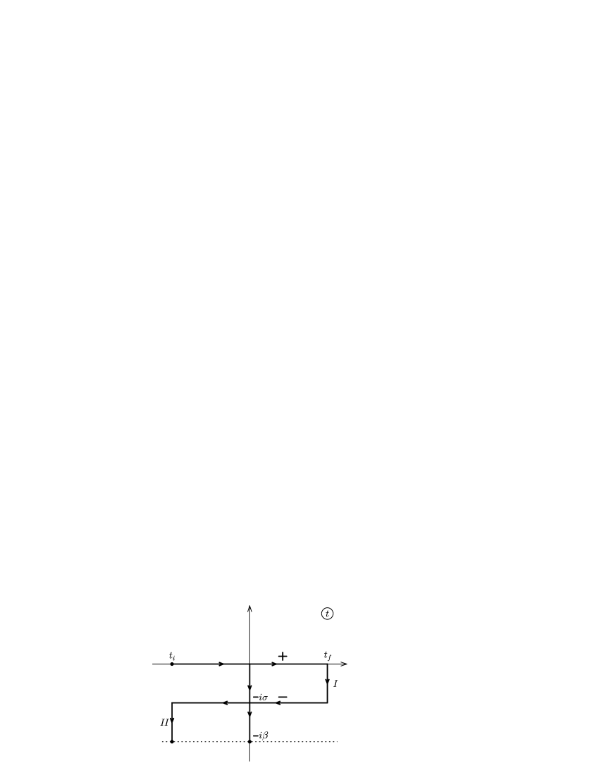
Figure 1: The contour for the time integration in the complex time plane for equilibrium systems. The value of $\sigma$ is usually chosen to be $\beta/2$. The initial time $t_{i}\to-\infty$ and the final time $t_{f}\to\infty$.

The thermodynamics of a system with variable fermion number density is determined by the grand potential $\Omega$ defined as

$$e^{-\beta\Omega} = Tre^{-\beta(\widehat{H}-\mu\widehat{N})},$$ (56)

where $\widehat{N}$ is the fermion number and $\widehat{H}$ is the Hamiltonian of the system. The grand potential $\Omega$ has a well known relation with other thermodynamical quantities in elementary thermodynamics, namely

$$\Omega=U-TS-\mu N$$ (57)

with $U$ the internal energy , $T$ the temperature, $S$ the entropy and $N$ the average particle number of the system.

In the quantum field theoretical investigation of the same system, there is another representation for the right hand side (r.h.s.) of Eq. 56 in terms of Feynman–Matthews–Salam (FMS) FMS path integration

$$Tre^{-\beta\widehat{K}}=const\times\int[D\psi][D\bar{\psi}]e^{-S_{E}},$$ (58)

where $\widehat{K}\equiv\widehat{H}-\mu\widehat{N}$, “$const$” is so chosen that $\Omega=0$ at zero temperature and density. $S_{E}$ is the Euclidean action of the system; it can be obtained from the Minkowski action for the system by a continuous change of the metric Mehta . For example, the action $S_{E}$ for a free fermion system is

$$S_{E}=\int d^{4}x\bar{\psi}\left(i\hbox to0.0pt{/\hss}\partial+\mu\gamma^{0}_{E}-m\right)\psi,$$ (59)

where $x^{\mu}$ is the (4-dim) Euclidean space-time coordinates, $\gamma_{E}^{0}=i\gamma^{5}$ and $m$ is the mass of the fermion. $\Omega$ is obtained by identifying $\beta$ with the interval $x_{4}$ (the Euclidean time) that the system is anti-periodic.

Since only “free” systems in which the Lagrangian for the fermion system is a bilinear form in the fermion field are considered in this section, the path integration can be carried out immediately. The standard procedure of doing the (imaginary) energy integration at zero temperature is replaced by a summation of the discrete Matsubara frequencies (energies) implied by Eq. 55. Such a boundary condition for $\psi$ results, however, in different analytic structure for the path integration from that for the FMS path integration in the real-time in the 4-component theory for fermions. This will be discussed in the following.

The grand potential in the Matsubara formalism is

$$\Omega = -\mbox{Sp}\mbox{Ln}\gamma_{E}^{0}\left(i\hbox to0.0pt{/\hss}\partial+\mu\gamma_{E}^{0}-m\right)-\Delta\Omega$$ (60)

$$= -\frac{2V}{\beta}\int\frac{d^{3}p}{(2\pi)^{3}}\sum_{n=-\infty}^{\infty}\ln\left\{m^{2}+\mbox{\boldmath{$p$}}^{2}-\left[i(2n+1)\pi\beta^{-1}+\mu\right]^{2}\right\}-\Delta\Omega,$$

where “Sp” denotes the functional trace and $\Delta\Omega$ is so chosen that $\Omega(T=\mu=0)=0$. The summation over Matsubara frequencies can be evaluated by expressing it as a contour integration in the complex energy plane, namely,

$$\Omega=-2V\int\frac{d^{3}p}{(2\pi)^{3}}\int_{C_{0}}\frac{dz}{2\pi i}\left[\mbox{tanh}(\frac{1}{2}\beta z)f(z,\mu)-\lim_{\beta\rightarrow\infty}\mbox{tanh}(\frac{1}{2}\beta z)f(z,0)\right],$$ (61)

where $C_{0}$ is shown in Fig. 2 and

$$f(z,\mu)=\ln\left[m^{2}+\mbox{\boldmath{$p$}}^{2}-(z+\mu)^{2}\right].$$ (62)

Figure 2: The set of contours for the imaginary-time approach to thermodynamics using thermal field theory. Contour $C_{0}$ encloses the Matsubara poles of the integrand. Contours $C_{+}$ and $C_{-}$ are the ones needed in a real time formulation of the thermal field theory in the 4 component representation for fermion fields.

Since the integrand of the $z$ integration approaches to zero fast enough in the $|z|\rightarrow\infty$ limit and is analytic in the complex $z$ plane excluding the real and imaginary axis, the integration over $z$ along contour $C_{0}$ is equivalent to the sum of integration along contours $C_{+}$ and the negative of $C_{-}$ of Fig. 2. The internal energy $U$, entropy $S$ and the particle number $N$ of the system extracted from $\Omega$ according to pattern Eq. 57 are

$$U = \frac{V}{\pi^{2}}\int_{0}^{\infty}d\mbox{\boldmath$p$}\mbox{\boldmath$p$}^{2}\left[f^{(-)}_{\mathbf{p}}+f^{(+)}_{\mathbf{p}}\right]E_{\mathbf{p}},$$ (63)

$$S = S^{(+)}+S^{(-)},$$ (64)

$$S^{(\pm)} = -\frac{V}{\pi^{2}}\int_{0}^{\infty}d\mbox{\boldmath$p$}\mbox{\boldmath$p$}^{2}\left[f^{(\pm)}_{\mathbf{p}}\ln f^{(\pm)}_{\mathbf{p}}+\left(1-f^{(\pm)}_{\mathbf{p}}\right)\ln\left(1-f^{(\pm)}_{\mathbf{p}}\right)\right],$$ (65)

$$N = \frac{V}{\pi^{2}}\int^{\infty}_{0}d\mbox{\boldmath$p$}\mbox{\boldmath$p$}^{2}\left[f^{(-)}_{\mathbf{p}}-f^{(+)}_{\mathbf{p}}\right]$$ (66)

with $E_{\mathbf{p}}=\sqrt{\mbox{\boldmath$p$}^{2}+m^{2}}$ and

$$f^{(\pm)}_{\mathbf{p}}=\frac{1}{e^{\beta(E_{\mathbf{p}}\pm\mu)}+1}$$ (67)

the Fermi–Dirac distribution for fermionic particles and antiparticles respectively. These quantities are in agreement with elementary statistical mechanics.

III.2 Real-time formulation of the thermal field theory

One of the non-perturbative treatments of the relativistic quantum field theory is based upon the FMS path integration in real-time FMS . The FMS formalism expresses time evolution between initial and final states in terms of an integration over paths that connect the initial and final states with a weight determined by the action of each particular path. The results of the path integration at the formal level are not uniquely defined in the Minkowski space-time due to the presence of singularities. Their uniqueness is determined by the fact that the derivation of the FMS path integration representation of the evolution operator implies a particular ordering of the intermediate states which defines how the singularities of the formal results are handled. The FMS causal structure, which provides one of the Lorentz invariant prescriptions, determines the particle content of the quantum fields. It requires that particles are positive energy solution of the Dirac equation (or corresponding non-relativistic equation in condensed matter systems with its energy defined relative to the Fermi surface of the system) that propagate forward in time and antiparticles (or holes) are the negative energy solution that effective “propagate backward in time”. In fact the canonical quantization of the quantum field is possible only after such a classification of the solution of the classical “wave equation”. The great success of the quantum field theory in such a causal structure for real-time processes at zero density leaves almost no room for any alternation of it. Thus the path integration formalism is defined by not only the formal expressions that contain singularities but also by the “causal structure” following the time ordering of the physical intermediate states.

The dynamical evolution of a system in more general situations including the finite density ones has also to be studied in such a real-time formulation of the quantum field theory. Consistency requires that the results of such a formulation to agree with the results from the imaginary-time formulation when it is applied to the equilibrium situations. The question is whether or not it actually happens, especially for fermions.

III.2.1 Fermion propagator in finite temperature theory

For the fermions interested in this study, the boundary condition Eq. 55 can be expressed as $\widehat{\Psi}(t)=-e^{\beta\widehat{K}}\widehat{\Psi}(t)e^{-\beta\widehat{K}}$. It is equivalent to Eq. 55 due to the fact that the conserved $\widehat{N}$ commutes with the total Hamiltonian $\widehat{H}$, which allows the factorization of the action of $\beta\mu\widehat{N}$ and $\beta\widehat{H}$ in the exponential of $\beta\widehat{K}$. The $\exp(\beta\mu O_{3})$ factor in Eq. 55 is the result of the action of $\exp(\beta\mu\widehat{N})$ and $\exp(-\beta\mu\widehat{N})$ on both side of $\Psi$. The commutativity of $\widehat{H}$ and $\widehat{N}$ shall not be imposed at this level of development but rather at later stages as dynamical constraints.

The real-time thermal field dynamics in the 8-component representation for fermion fields can be constructed along the same line as that of, e.g., Refs. LandsWeer ; Kapusta ; RTTFD1 ; RTTFD2 ; RTTFD3 ; Shuyak . The formal differences of the present approach against those developments are 1) the Kubo–Martin–Schwinger (KMS) boundary condition for the contour propagator do not contain the $\exp(\beta\mu)$ factor in the present approach, the effects of $\mu$ is hidden in the energy variable within the propagator (namely, the time evolution is generated by $\widehat{K}$ not $\widehat{H}$) here, 2) the Feynman rules in a perturbation expansion is different from the 4-component theory and 3) the analytic properties of the present approach in the complex energy plane is different from some of the earlier ones of this field.

The matrix form of contour propagator for a fermion is

$${\cal S}(p) = M\left(\begin{array}[]{cc}S^{+}(p)&0\\ 0&S^{-}(p)\end{array}\right)M,$$ (70)

where the retarded and advanced propagators $S^{+}$ and $S^{-}$ are

$$S^{\pm}(p)=\frac{\pm i}{\hbox to0.0pt{/\hss}p+\gamma^{0}\mu O_{3}-mO_{3}\pm i\gamma^{0}\epsilon}$$ (71)

and

$$M=\left(\begin{array}[]{cc}\sqrt{1-n(p_{0})}&-\sqrt{n(p_{0})}\\ &\\ \sqrt{n(p_{0})}&\sqrt{1-n(p_{0})}\end{array}\right)$$ (72)

with

$$n(e)=\frac{1}{e^{\beta e}+1}.$$ (73)

It is easy to show that ${\cal S}_{11}(p)\to S_{F}(p)$ in the zero temperature limit since the energy ($p_{0}$) poles of it are located above the contour $C_{FMS}$ if they are negative and below it otherwise. It can be compared to the conventional real-time approach with the correct causal structure Shuyak ; Lutz at zero temperature, in which the poles of the fermion propagator are located above the $p_{0}$ integration contour if they are on the left of $\mu$ or else below it.

There is at least another way to realize the KMS boundary condition. The choice of Feynman propagators and its complex conjugation is adopted instead of the retarded and advanced ones to express ${\cal S}(p)$ in some of the earlier literatures of the field. In such a choice, the matrix $M$ as a function of $p^{0}$ can not be analytically continued into the complex $p^{0}$ plane. It therefore has bad analytic properties.

The transformation matrix $M$ (Eq. 72) is determined by the KMS boundary condition. It is therefore independent of the detailed dynamics of the system and satisfies

$$M\eta M=\eta,$$ (74)

where the matrix

$$\eta=\left(\begin{array}[]{cc}1&0\\ 0&-1\end{array}\right)$$ (75)

is a matrix acting on the same space as $M$ does.

III.2.2 The effective or grand potential

The grand potential or the effective potential of a free fermionic system in the present approach is

$$\Omega=-\lim_{\Delta t\rightarrow\infty}\frac{i}{2\Delta t}\mbox{Sp}\left[\mbox{Ln}\gamma^{0}\eta{\cal S}\right]_{11}-\Delta\Omega,$$ (76)

where Sp denotes the functional trace, $\Delta t=t_{f}-t_{i}$ (see Fig. 1) and $\Delta\Omega$ is a constant that makes $\Omega$ to vanish in the zero temperature and density limit. The subscript “11” means that the first diagonal matrix element of the operator in the square bracket of Eq. 76 within the $2\times 2$ space of the real-time theory for finite temperature should be taken. Using the propagator Eq. 70 and the property Eq. 74 for the matrix $M$, it is easy to show that the functional trace in this case can be carried out in the 4-momentum space and

$$\Omega=-\frac{i}{2}V\int\frac{d^{3}p}{(2\pi)^{3}}\int\frac{dp_{0}}{2\pi}\mbox{Tr}\left[M^{2}_{11}\mbox{Ln}\gamma^{0}S^{+}(p)-M_{12}M_{21}\mbox{Ln}\gamma^{0}S^{-}(p)\right]-\Delta\Omega.$$ (77)

For a free theory the retarded/advanced propagators $S^{\pm}(p)$ are given in Eq. 71. The resulting $\Omega$ is

$$\Omega = iV\int\frac{d^{3}p}{(2\pi)^{3}}\left\{\int_{C_{R}}\frac{dp_{0}}{2\pi}\left[1-n(p_{0})\right]\ln(p_{+}^{2}-m^{2})(p_{-}^{2}-m^{2})\right.$$ (78)

$$\hskip 56.9055pt+\left.\int_{C_{A}}\frac{dp_{0}}{2\pi}n(p_{0})\ln(p_{+}^{2}-m^{2})(p_{-}^{2}-m^{2})-2\int_{C_{FMS}}\frac{dp_{0}}{2\pi}\ln(p^{2}-m^{2})\right\},$$

with $p_{\pm}^{\mu}=\{p^{0}\pm\mu,\mbox{\boldmath{$p$}}\}$, the contour $C_{R}$ running above the real $p_{0}$ axis and contour $C_{A}$ running below the real $p_{0}$ axis. Since the logarithmic functions in the above equation is well behaved at large $|p_{0}|$ in the complex $p_{0}$ plane for the 8-component theory, as it is discussed in detail in the following, the integration contour for $p_{0}$ can be deformed to $C_{0}$ of Fig. 2. It can be shown that Eq. 78 is exactly the same as Eq. 61. Some of the technical points are discussed in the following.

Thus the real-time approach using an 8-component “real” representation for fermions is equivalent to the conventional imaginary-time theory. Therefore it give us correct thermodynamics without additional subtraction terms. Such an equivalence is not present in the conventional real-time formulation of the thermal field theory in the 4-component representation for fermions. It is demonstrated in the following.

III.3 The zero temperature limit of the real-time theory

The difference between the 4-component theory and the 8-component one for fermions manifest in the zero temperature limit already.

The 4-component theory for the grand potential in the real-time formulation of the finite density problem at zero density is given ThPap ; ThPap2 by

$$\Omega = \lim_{\Delta t\rightarrow\infty}\frac{i}{\Delta t}\mbox{Sp}\mbox{Ln}\gamma^{0}\left(i\hbox to0.0pt{/\hss}\partial+\mu\gamma^{0}-m\right)+\mbox{const}$$ (79)

$$= 2iV\int\frac{d^{3}p}{(2\pi)^{3}}\int_{C_{FMS}}\frac{dp^{0}}{2\pi}\ln\frac{p_{+}^{2}-m^{2}}{p^{2}-m^{2}},$$ (80)

where $C_{FMS}$ is the $p^{0}$ integration contour for the FMS causal structure shown in Fig. 3.

Figure 3: The set of contours belonging to the same FMS class. Contour $C_{FMS}$ is the original FMS contour in the Minkowski space. Contour $C_{E}$ is the Euclidean contour. Contour $C_{+}$ is the quasiparticle contour. $\pm i\pi$ denote the imaginary part of the integrand along the edges of its cuts (thick lines) on the physical $p_{0}$ plane.

There are also a pair of contours $C_{+}$ and $C_{-}$ in Fig. 2, called the quasiparticle contour ThPap , that contribute to the real-time response of the system in the $\beta\rightarrow\infty$ limit. Contours $C_{FMS}$, $C_{E}$, $C_{+}$ and $C_{-}$ in Fig. 2 belong to the same topological class of contours having the same FMS causal structure. The integration on $C_{E}$ leads to the correct thermodynamics as shown in the above subsection. Consistency requires the equivalence of the set of contours $C_{FMS}$, $C_{E}$, $C_{+}$ and $C_{-}$ for the physical quantities. Eq. 80 unfortunately fails to meet this requirement due to the fact that the imaginary part of the logarithmic function falls off as $O(\mu/|p_{0}|)$ on the physical $p_{0}$ sheet. This makes the results obtained by doing the $p_{0}$ integration on the above mentioned set of contours different from each other since the integration on the large circle sections of the contour has a non-vanishing value. It is not difficult to verify that while integrating along $C_{E}$ produces the correct thermodynamics, explicit computation of Eq. 80 on contour $C_{+}$ or $C_{-}$ on which only the imaginary part of the integrand contributes (see Fig. 3), yields a form differs from the finite value $\Omega=U-\mu N$. It actually diverges.

The origin of the above mentioned problems can be traced back to the asymmetric nature of the 4-component representation of the fermion fields with respect to particles and antiparticles in the Minkowski space-time. If one compares Eq. 61 in the $\beta\rightarrow\infty$ limit and Eq. 80, after a distortion of contour $C_{0}$ to $C_{+}$ and the negative of $C_{-}$ in Fig. 2, one finds that Eq. 80 differs from Eq. 61 by the lack of the contribution from the integration along the negative of contour $C_{-}$, which has to be present for the finiteness of the result.

However the integration contour along the negative of $C_{-}$ is absent for the real-time dynamical evolution of the system according to the FMS causal structure. There seems to be no way of getting a finite result that agrees with thermodynamics in the 4-component theory without at lease one arbitrary subtraction in addition to the zero density and temperature ones.

The large energy behavior of the 8-component theory for fermions is better. The grand potential at zero temperature in the 8-component theory is given by the $\beta\to\infty$ limit of Eq. 78, which is

$$\Omega = iV\int\frac{d^{4}p}{(2\pi)^{4}}\ln\frac{(p_{+}^{2}-m^{2})(p_{-}^{2}-m^{2})}{(p^{2}-m^{2})^{2}}$$ (81)

with the same order of integration as Eq. 80. Here $p_{\pm}^{\mu}=(p^{0}\pm\mu,\mbox{\boldmath$p$})$. Eq. 81 and Eq. 80 have an identical value on the contour $C_{E}$. They differ on contours $C_{\pm}$ because the large $p_{0}$ behavior of the imaginary part of the logarithmic function in Eq. 81 is of order $O(\mu^{2}/|p_{0}|^{2})$ on the physical sheet, which guarantee the equivalence between the set of contours $C_{FMS}$, $C_{E}$, $C_{+}$ and $C_{-}$. By following the $C_{+}$ contour shown in Fig. 3, it is simple to show that the resulting right hand side of Eq. 81 is finite and unique, namely, $U-\mu N$. It is the zero temperature grand potential for a free fermion system at density $\overline{n}=N/V$ expected from thermodynamics.

In the 8-component theory for fermions, the above mentioned effects of the $C_{-}$ are provided by the lower 4 component $\psi_{2}$ of $\Psi$.

III.4 Lorentz covariance and ground state expectation of local observables

Let us turn to the study of the ground state expectation of local bilinear operators constructed from two fermion fields of the form

$$\widehat{O}=\overline{\Psi}(x)\Gamma\Psi(x)$$ (82)

in a finite density environment where $\Gamma$ is certain matrix acting on $\Psi$. A local product of two field operators is in general singular and non-unique. The usual procedure of normal ordering depends on the Fock space in which the particles of the corresponding “non-interacting” Lagrangian is represented. In strong interaction, these particles, like the current quarks, may never appear in the asymptotic spectra of the full theory. In addition, there is a non-perturbative spontaneous chiral symmetry breaking in the vacuum state, which generates a much larger mass for the quarks. It makes a unique definition of the normal ordering for strong interaction theories quite difficult.

A definition of such a potentially divergent product that is independent of the dynamics of the system is

$$\widehat{O}=\lim_{\delta_{\mu}\rightarrow 0}\overline{\Psi}(x+\delta)\Gamma\Psi(x),$$ (83)

where $\delta_{\mu}$ is a 4-vector with, e.g., $\delta_{0}<0$. The ground state (vacuum) expectation value of $\widehat{O}$ can thus be computed from the fermion propagator ${\cal S}$

$$<\widehat{O}> = -\mbox{tr}\int\frac{d^{3}p}{(2\pi)^{3}}\int_{C_{R}}\frac{dp_{0}}{2\pi}{\cal S}^{11}(p)\Gamma,$$ (84)

with “tr” denoting the trace over internal indices of the fermion fields and

$${\cal S}^{11}=\left[1-n(p^{0})\right]S^{+}(p)-n(p^{0})S^{-}(p).$$ (85)

Since there is no poles and cuts off the real $p_{0}$ axis except the ones on the imaginary $p_{0}$ axis due to the thermal factor, which should be excluded (see Fig. 2), contour $C_{R}$ can be closed in the lower half plane to include the poles of the retarded propagator $S^{+}$. So, Eq. 84 is reduced to

$$<\widehat{O}> = i\int\frac{d^{3}p}{(2\pi)^{3}}\sum_{k}[1-n(p^{0}_{k})]\mbox{tr}\mbox{Res}S^{+}(p_{k})\Gamma,$$ (86)

where the sum is over all poles $p^{0}_{k}$ of $S^{+}(p)$ and “Res” denotes the corresponding residue. The difference between the 8-component theory and the 4-component one also manifests here. For example, the conserved fermion number density $\overline{n}$ corresponding to current

$$j^{\mu}=V_{I}^{\mu}=\frac{1}{2}\overline{\Psi}\gamma^{\mu}O_{3}\Psi$$ (87)

is

$$\overline{n}={1\over\pi^{2}}\int^{\infty}_{0}d\mbox{\boldmath$p$}\mbox{\boldmath$p$}^{2}\left[f^{(-)}_{\mathbf{p}}-f^{(+)}_{\mathbf{p}}\right].$$ (88)

It is same as the one in elementary statistical mechanics.

If we choose $\delta_{0}>0$, then the contributing component of ${\cal S}^{11}$ is the advanced propagator $S^{-}$

$$<\widehat{O}> = -i\int\frac{d^{3}p}{(2\pi)^{3}}\sum_{k}n(p^{0}_{k})\mbox{tr}\mbox{Res}S^{-}(p_{k})\Gamma.$$ (89)

It is the same as Eq. 86. It also tells us that the choice made in Eq. 48 is the right one. This is because if we choose “type–II” operators for the fermion number density instead, the result is divergent.

On the other hand, $\overline{n}$ computed in the 4-component theory using such a point split definition of fermion number density is divergent and different from each other for $\delta_{0}>0$ and $\delta_{0}<0$. It means that it is not even consistent with relativity for a space like $\delta_{\mu}$ whose time component can has different sign in different reference frames. It can be made finite and unique only after an arbitrary subtraction that depends on the reference frame. It is another serious conceptual problem originated from the non-commutativity of quantum mechanical quantities and the relativistic space-time. Such a conflict between quantum mechanics and relativity is avoidable only in the 8-component theory for fermions.

IV Quantization and Particle Interpretation

The language used so far is the path integration one which treats the fermion fields as Grassmanian numbers. Such a representation of the problem is most useful in discussing the wave aspects of the problem. In most experimental observations, especially in high energy physics in which only a small number of particles are involved in a reaction, the particle aspect of the problem has to be understood. In such a case, the physics is most easily described in terms of the Fock space of the problem in the operator language.

IV.1 Free particles

The particle content of the 8-component theory can be found by first studying the pole structure of the fermion propagator under the FMS causal condition. The time dependence of the propagator (see section III) at zero temperature is

$$\lim_{\beta\rightarrow\infty}{\cal S}_{11}(t,\mbox{\boldmath$p$})=S_{F}(t,\mbox{\boldmath$p$})=\int_{C_{FMS}}\frac{dp_{0}}{2\pi}e^{-ip_{0}t}S_{F}(p_{0},\mbox{\boldmath$p$}).$$ (90)

In case of $t>0$, Eq. 90 can be evaluated on the contour $C_{+}$ of Fig. 2 by closing the integration contour in the lower half $p_{0}$ plane

$$S_{F}(t,\mbox{\boldmath$p$}) = \theta(E_{\mathbf{p}}-\mu)\Lambda^{1+}_{\mathbf{p}}e^{-i(E_{\mathbf{p}}-\mu)t}+\theta(\mu-E_{\mathbf{p}})\Lambda^{2-}_{\mathbf{p}}e^{-i(\mu-E_{\mathbf{p}})t}+\Lambda^{2+}_{\mathbf{p}}e^{-i(E_{\mathbf{p}}+\mu)t}$$ (91)

and, if $t<0$, can be evaluated on the contour $C_{-}$ to obtain

$$S_{F}(t,\mbox{\boldmath$p$}) = \Lambda^{1-}_{\mathbf{p}}e^{i(E_{\mathbf{p}}+\mu)t}+\theta(\mu-E_{\mathbf{p}})\Lambda^{1+}_{\mathbf{p}}e^{i(\mu-E_{\mathbf{p}})t}+\theta(E_{\mathbf{p}}-\mu)\Lambda^{2-}_{\mathbf{p}}e^{i(E_{\mathbf{p}}-\mu)t}.$$ (92)

Here

$$\Lambda_{\mathbf{p}}^{r\pm}=P_{r}\frac{(\pm\gamma^{0}E_{\mathbf{p}}-\mbox{\boldmath$\gamma$}\cdot\mbox{\boldmath$p$}+mO_{3})}{2E_{\mathbf{p}}},$$ (93)

$P_{1}=(1+O_{3})/2$, $P_{2}=(1-O_{3})/2$ are projection operators and $r=\{1,2\}$.

The FMS causal structure in the present theory can be simply putted as: 1) excitations with $p_{0}>0$ that propagate forward in time correspond to particles and 2) those with $p_{0}<0$ that propagate backward in time correspond to antiparticles. Fig. 4 shows the spectra for particles and antiparticles at finite density with $\mu>m$, where lines $a$, $\overline{b}$ and $\overline{c}$ are contributions from the $r=1$ excitations and lines $\overline{a}$, $b$ and $c$ are contributions from the $r=2$ ones.

Figure 4: A schematic plot of the spectra for fermions in the 8-component theory when $\mu>m$. The solid lines above zero (of $p^{0}$ in the propagator) correspond to particles and the dashed line below zero correspond antiparticles. The $p^{0}=0$ surface correspond to the Fermi surface.

The quantization of the 8-component fermionic field then follows naturally. $\widehat{\Psi}(x)$ can be written as

$$\widehat{\Psi}(x) = \sum_{r\mathbf{p}s}\frac{1}{2E_{\mathbf{p}}}\left[U_{r\mathbf{p}s}e^{-i\theta({\bf p})\widetilde{p}\cdot x}\widehat{B}_{r\mathbf{p}s}(t)+V_{r\mathbf{p}s}e^{i\theta({\bf p})\widetilde{p}\cdot x}\widehat{D}^{\dagger}_{r\mathbf{p}s}(t)\right],$$ (94)

where when $\mu>m$,

$$\widehat{B}_{1\mathbf{p}s}(t)=\left\{\begin{array}[]{cr}e^{i\mu t}\widehat{b}_{1\mathbf{p}s}&\hskip 8.5359pt\mbox{if $|{\bf p}|>p_{F}$}\\ e^{-i\mu t}\widehat{b}_{1\mathbf{p}s}^{\dagger}&\hskip 8.5359pt\mbox{if $|{\bf p}|<p_{F}$}\end{array}\right. \widehat{B}_{2\mathbf{p}s}(t)=e^{-i\mu t}\widehat{b}_{2\mathbf{p}s}$$ and (97)

$$\widehat{D}^{\dagger}_{2\mathbf{p}s}(t)=\left\{\begin{array}[]{cr}e^{i\mu t}\widehat{d}^{\dagger}_{2\mathbf{p}s}&\hskip 8.5359pt\mbox{if $|{\bf p}|>p_{F}$}\\ e^{-i\mu t}\widehat{d}_{2\mathbf{p}s}&\hskip 8.5359pt\mbox{if $|{\bf p}|<p_{F}$}\end{array}\right. \widehat{D}^{\dagger}_{1\mathbf{p}s}(t)=e^{-i\mu t}\widehat{d}^{\dagger}_{1\mathbf{p}s}$$ and (100)

with $p_{F}=\sqrt{\mu^{2}-m^{2}}$ and $\theta({\bf p})=\mbox{sign}(|{\bf p}|-p_{F})$. Here $s$ is the spin index, the 4-momentum $\widetilde{p}^{\mu}=\{E_{\bf p},{\bf p}\}$, $U_{r\mathbf{p}s}$ and $V_{r\mathbf{p}s}$ are 8-component spinors that satisfy

$$(\hbox to0.0pt{/\hss}{\widetilde{p}}-mO_{3})U_{r\mathbf{p}s} = 0,$$ (101)

$$(\hbox to0.0pt{/\hss}{\widetilde{p}}+mO_{3})V_{r\mathbf{p}s} = 0.$$ (102)

Their solution can be easily found

$$U_{1\mathbf{p}s}=\left(\begin{array}[]{c}u(\mathbf{p}s)\\ 0\end{array}\right), U_{2\mathbf{p}s}=\left(\begin{array}[]{c}0\\ v(\mathbf{p}s)\end{array}\right),$$ (107)

$$V_{1\mathbf{p}s}=\left(\begin{array}[]{c}v(\mathbf{p}s)\\ 0\end{array}\right), V_{2\mathbf{p}s}=\left(\begin{array}[]{c}0\\ u(\mathbf{p}s)\end{array}\right)$$ (112)

with $u(\mathbf{p}s)$ and $v(\mathbf{p}s)$ the conventional Dirac spinors for particles and antiparticles respectively in the 4-component theory. It can be seen that the two $U$s with the same quantum numbers besides $r$ map into each other under the mirror reflection transformation so do the two $V$s.

The non-vanishing anticommutators between $\widehat{b}_{r\mathbf{p}s}$ and $\widehat{d}_{r\mathbf{p}s}$ in the canonical quantization of the fermion fields are

$$\left\{\widehat{b}_{r\mathbf{p}s},\widehat{b}^{\dagger}_{r^{\prime}\mathbf{p}^{\prime}s^{\prime}}\right\} = 2E_{\mathbf{p}}\delta_{\mathbf{pp}^{\prime}}\delta_{ss^{\prime}}\delta_{rr^{\prime}},$$ (113)

$$\left\{\widehat{d}_{r\mathbf{p}s},\widehat{d}^{\dagger}_{r^{\prime}\mathbf{p}^{\prime}s^{\prime}}\right\} = 2E_{\mathbf{p}}\delta_{\mathbf{pp}^{\prime}}\delta_{ss^{\prime}}\delta_{rr^{\prime}}.$$ (114)

They realize a canonical quantization of $\widehat{\Psi}$.

IV.2 The constraint of the reality condition

Since the mirror reflection operations defined in Eqs. 21 and 22 involve time reversal transformation, it is necessary to discuss the time reversal transformation on operators in the Hilbert space in some details first.

IV.2.1 The causal and motion reversal of time

There are two kinds of statement for time reversal transformation of the matrix elements thesis of a operator. The first one is the so called causal reversal transformation which involves the interchange of initial and final states together with the motion reversal of the quantum numbers, like the 3–momentum, $z$–component of the angular momentum, etc., of the initial and the final states. Namely

$$<f|\widehat{O}|i>\stackrel{{\scriptstyle\widehat{\cal T}_{c}}}{{\longrightarrow}}<\widetilde{i}|\widehat{O}|\widetilde{f}>$$ (115)

with the tilde states the corresponding motion reversed one. The second one is the so called motion reversal transformation which is defined by

$$<f|\widehat{O}|i>\stackrel{{\scriptstyle\widehat{\cal T}_{m}}}{{\longrightarrow}}<\widetilde{f}|\widehat{O}|\widetilde{i}>^{*},$$ (116)

which contains a complex conjugation but does not exchange the initial and final states. These two definitions are equivalent only for Hermitian operators.

The genuine test of time reversal invariance involves causal reversal of time thesis ; cern1 because it can be shown that the signals in the motion reversal test of time reversal invariance could be contaminated by pseudo time reversal violation effects thesis ; EMH-ME due to final state interaction.

The operator form of causal reversal of time given by Eq. 115 is

$$\widehat{\cal T}_{c}\widehat{O}\widehat{\cal T}^{-1}_{c}=\widehat{U}\widehat{O}^{T}\widehat{U}^{\dagger}$$ (117)

with superscript “T” denoting the transpose of the operator and $\widehat{U}$ an unitary operator that maps a state $|\phi>$ to its motion reversed state $|\widetilde{\phi}>$.

For the fermion field operator $\widehat{\Psi}$, the operator causal time reversal transformation corresponding to Eq. 9 is

$$\widehat{\Psi}({\bf x},t)\stackrel{{\scriptstyle\widehat{\cal T}}}{{\longrightarrow}}\gamma^{0}\gamma^{5}iO_{2}\widehat{\Psi}^{T}({\bf x},-t),$$ (118)

where the transpose on the right hand side is only on the operators $\widehat{b}$s and $\widehat{d}$s but not on the Dirac indices. From Eq. 94, taking into account that the time reversal transformation is an anti-linear transformation, Eq. 118 is equivalent to

$$\widehat{b}_{1\mathbf{p}s}\stackrel{{\scriptstyle\widehat{\cal T}}}{{\longrightarrow}}\widehat{b}_{2-\mathbf{p}-s}^{T}, \widehat{b}_{2\mathbf{p}s}\stackrel{{\scriptstyle\widehat{\cal T}}}{{\longrightarrow}}\widehat{b}_{1-\mathbf{p}-s}^{T},$$ (119)

$$\widehat{d}_{1\mathbf{p}s}\stackrel{{\scriptstyle\widehat{\cal T}}}{{\longrightarrow}}\widehat{d}_{2-\mathbf{p}-s}^{T}, \widehat{d}_{2\mathbf{p}s}\stackrel{{\scriptstyle\widehat{\cal T}}}{{\longrightarrow}}\widehat{d}_{1-\mathbf{p}-s}^{T}.$$ (120)

IV.2.2 The constraint of the reality condition

The operator representation of the mirror reflection operation defined in Eq. 21 on $\widehat{\Psi}$ is then realized by

$$\widehat{b}_{1\mathbf{p}s}\stackrel{{\scriptstyle\widehat{\cal M}}}{{\longrightarrow}}\widehat{b}_{2\mathbf{p}s}^{*}, \widehat{b}_{2\mathbf{p}s}\stackrel{{\scriptstyle\widehat{\cal M}}}{{\longrightarrow}}\widehat{b}_{1\mathbf{p}s}^{*},$$ (121)

$$\widehat{d}_{1\mathbf{p}s}\stackrel{{\scriptstyle\widehat{\cal M}}}{{\longrightarrow}}\widehat{d}_{2\mathbf{p}s}^{*}, \widehat{d}_{2\mathbf{p}s}\stackrel{{\scriptstyle\widehat{\cal M}}}{{\longrightarrow}}\widehat{d}_{1\mathbf{p}s}^{*}.$$ (122)

So the reality condition at zero density is

$$\widehat{b}_{1\mathbf{p}s}=\widehat{b}^{*}_{2\mathbf{p}s},\hskip 28.45274pt\widehat{d}_{1\mathbf{p}s}=\widehat{d}^{*}_{2\mathbf{p}s}.$$ (123)

These conditions for the Fock space are almost trivial to implement as long as the matrix elements of annihilation operator $\widehat{b}$s and $\widehat{d}$s are chosen to be real number and they are renormalized in the same way in interacting systems.

IV.3 Feynman rules for elementary processes and the reality condition

Although the 8-component theory for fermion contains twice as many degrees of freedom as the 4-component one, it is shown in the discussion of the previous sections, especially in section III, all of these excitation modes should be taken into account in order to obtain correct counting of states due to the $1/2$ factors contained in the free Lagrangian and in the interaction vertices.

The properties of the ground state, like the grand potential, the fermion number density and the scalar charge density are all computed using the quark propagator that contains external background fields, collectively denoted as $f$, like the chemical potential $\mu$ (or the statistical gauge field in the local theory ThPap ; ThPap2 ), the scalar field $\sigma$, etc.. In fact each set of these background fields has a corresponding set of positive energy ($p^{0}$ in the propagator) and negative energy excitation modes and therefore a corresponding temporary ground state for the fermion sector of the system. The properties of the ground state in the background field $f$ for the fermion sector is obtained by summing over the contributions of individual excitation modes with negative energy. In the true ground state of the whole system, including the boson sector, the external field takes certain value $\overline{f}$, which is called the classical configuration that stabilizes the system.

The elementary processes concerns the local excitations of the system above the ground state (positive $p^{0}$ events) in the external field configuration $\overline{f}$, which is the stable configurations of the whole system including the external source. They are treated differently from the ground state properties. The quantum fluctuation part of the bosonic fields $\delta f=f-\overline{f}$ does not enter the fermion propagator in the perturbative expansion of the reaction amplitude of elementary processes. The central question here is how to implement the anti-linear reality condition Eq. 25 for quantized $\delta f$.

The general one particle spinor satisfies the 8-component Dirac equation which can be written as Eq. 135 in general with $\Sigma$ subject to constraint Eq. 30. Suppressing the spin and the ones corresponding to internal symmetries, there are four kinds of solutions. Two solutions $\Psi_{1}$ and $\Psi_{2}$ with positive energy and corresponding two solutions with negative energy. In the computation of physical reaction amplitude at zero density, one should choose one of the solutions from these two, say $\Psi_{1}$ (or $\Psi_{2}$, it does not matter which one is chosen.) the reality condition generates the other solution by using the mirror transformation $\widehat{\cal M}$ on $\Psi_{1}$, which is denoted as $\Psi_{1{\cal M}}$. At the one particle level, $\Psi_{1{\cal M}}$ is identical to $\Psi_{2}$. Therefore it seems that one can simply sum over $\Psi_{1}$ and $\Psi_{2}$ to get the final results. This is not always right due to the fact that the mirror transformation is an anti-linear transformation so that although the single particle matrix element $\Psi_{1{\cal M}}$ is identical to $\Psi_{2}$, they lives in different time zone. Using the causal time reversal representation of $\widehat{\cal M}$ discussed above (one can not use the motion reversal representation since the complex conjugation contained in it can modifies the causal structure of the fermion propagators leaving the effects of pseudo-time reversal violation thesis ), combined with Eqs. 49, 50 and 54, it can be shown that the interaction vertices inside of a Feynman graph is obtained from the interaction terms in Lagrangian density, which is denoted as $\Gamma$, by doing the following transformation

$$\widetilde{\Gamma}=\Theta\Gamma,$$ (124)

where $\widetilde{\Gamma}$, $\Gamma$ and $\Theta$ are $2\times 2$ matrices in the upper and lower 4-component space of $\Psi$ and

$$\Theta=\left(\begin{array}[]{cc}1&0\\ 0&\pm(-1)^{\nu}\end{array}\right)$$ (125)

with $\pm$ sign corresponding to a vertex of “type–I” or “type–II” respectively, where $\nu$ is the number of Lorentz indices on the vertices. Using $\widetilde{\Gamma}$ one can use $\Psi_{1}$ and $\Psi_{2}$ or the propagator $S_{F}$ to count the physical state in a way that respects the reality condition.

For situations in which $D=\overline{D}=0$ in the mass matrix $\Sigma$ (namely, Eq. 31), it can be shown that the value of the Feynman diagrams are the same as the conventional 4-component theory when $\mu=0$. For example, the one photon exchange electron–electron scattering amplitude contains three kinds of terms in the 8-component theory. They are $e-e$ scattering, $e-\widetilde{e}$ scattering and $\widetilde{e}-\widetilde{e}$ scattering terms, where $\widetilde{e}$ is the mirror electron. These terms are all identical and repulsive. If the reality condition is incorrectly imposed or not imposed at all, there can be $e-\widetilde{e}$ attraction leading to the bound $e\widetilde{e}$ pair that is not observed in Nature.

On may ask why $\Theta$ does not enter the expression for the grand potential and the ground state expectation value of local observables. The answer can be found if one carefully study the evaluation of the ground state expectation value of local observables. Each configuration of the background fields defines its own sets of particles and anti-particles since the spectra of $S^{-1}_{F}$ depend on it. In the background fields configuration $\overline{f}+\delta f$ some of the particles of in configuration $\overline{f}$ (positive energy solution) become antiparticles (negative solution) and vice versa. But perturbation theory is based on the particle content of configuration $\overline{f}$, $\delta f$ is treated as quantum fluctuations above the ground state and not included in the propagator, the factor the $(-1)^{\nu}$ is there to compensate for that. If $\delta f$ is included in the propagator in certain non-perturbative calculations like the lattice simulation, no $\Theta$ factor is needed, but in this case it is the “ground state” (in the presence of the external $\overline{f}+\delta f$ field) property that we are talking about then. As a rule, all vertices in a connected diagram that couple to a propagator of bosons should be written in terms of Eq. 124, only tadpoles type of vertices that couple to classical part of the boson fields or the background fields should use $\Gamma$ directly.

The reason why there is no such a factor in the 4-component theory is because the 4-component theory is “worse” than that by having divergences discussed in section III. The delicacies concerning the factor $(-1)^{\nu}$ needs not to be concerned since there are arbitrary infinities not present in the 8-component theory to be subtracted.

IV.4 Elementary processes at finite density

As it is mentioned above the 8-component theory is not equivalent to the 4-component theory at finite density, especially in relativistic many body systems. The differences can be traced back to the different behavior of the particles and their mirror partners in the finite density situations.

IV.4.1 The mirror particles

The positive energy excitation mode of the 4-component theory at finite density corresponds to the curve “a” of Fig. 4 only. The mirror partner of “a” in the 8-component theory are curves labeled by “b” and “c”. Excitation “c” is the mirror partner of “a” with respect to the Dirac sea since these two excitations become identical in the $\mu\to 0$ limit. It is separated from “a” by an energy difference $2\mu$ so that it is highly suppressed in non-relativistic conditions when $\beta m<<1$ with $\beta$ the inverse temperature and $m$ the mass of the excitation. Excitation “b” is the mirror excitation of “a” with respect to the Fermi sea. Due to asymmetric nature of the Fermi sea, excitation “b” is not identical to excitation “a” with respect to the Fermi surface. Only in the vicinity of the Fermi surface, both of them can be regarded as approximately identical since both of them have a linear spectra that is proportional to $|{\bf p}|-p_{F}$ with constant density of states. Here, $p_{F}$ is the Fermi momentum.

Besides the excitation spectra and density of states, the mutual interaction between particles is also different in the 8-component theory and in the 4-component theory. In order to find the difference let us find out the vector and scalar charges of the particles corresponding to spectra $a$, $b$ and $c$ and the antiparticles corresponding to spectra $\overline{a}$, $\overline{b}$ and $\overline{c}$ of Fig. 4.

The vector and scalar charge of a particle can be computed by taking the expectation value of the corresponding current between the zero momentum state of that particle. The result is given in Table 1.

Table 1: The scalar and vector charges of particles and antiparticles in the 8-component theory.

Excitations	aaaa $a$aaaa	aaaa$b$aaaa	aaaa $c$ aaaa	aaaa $\overline{a}$aaaa	aaaa $\overline{b}$aaaa	aaaa $\overline{c}$aaaaaa
Scalar Exchange	$1$	$-1$	$1$	$-1$	$1$	$-1$
Vector Exchange	$1$	$1$	$1$	$-1$	$-1$	$-1$

IV.4.2 The particle–particle scattering by exchange of vector bosons

In the 4-component theory for fermions at finite density, the excitation of the system corresponding to particles is given by line $a$ of Fig. 4. Let us denote the scattering amplitude between two excitations of “$a$” type in the 4-component theory by $T^{(4)}_{aa}$. The corresponding scattering processes in the 8-component theory is of three kind: $aa$, $bb$ and $ab$ (ignoring $c$ for the moment since it lies too high in energy to be significant in non-relativistic situations), therefore we have the following correspondence

$$T^{(4)}_{aa}\longleftrightarrow\frac{1}{4}\left(T_{aa}^{(8)}+T_{bb}^{(8)}+T_{ab}^{(8)}+T_{ba}^{(8)}\right),$$ (126)

where the $1/4$ factor is obtained by extracting the $1/2$ factor for the vertices of the 8-component theory. For the interaction induced by the exchange of vector bosonic particles like the photon, all four terms on the right hand side of correspondence (126) have the same sign since excitation “a” and “b” have the same vector charge. It can be shown that $T^{(4)}_{aa}$ and various $T^{(8)}_{aa,bb,ab,ba}$ also have the same form in terms of 4-component Dirac spinors $u(\mathbf{p}s)$. The only difference is that excitations “a” and “b”, which lives in different momentum domain, have different phase space volume. However, for condensed matter system like the electron gas in a metal only the excitations near the Fermi surface is important. In this case the density of states for both excitation “a” and “b” can be approximated by the density of state of the system at the Fermi surface, and Eq. 126 can be viewed as an approximate equation. So the non-relativistic condensed matter system of the above type in which the particle–particle interaction is dominated by the vector Coulomb interaction can not distinguish between the predictions of the 4-component theory and the 8-component theory when the density is sufficiently high.

IV.4.3 The particle–particle scattering by exchange of scalar bosons

Since the excitation mode “b” has different scalar charge from the excitation mode “a”, the predictions of the 8-component theory and the 4-component theory for fermion–fermion scattering through the exchange of scalar particles in finite density system is different since the prediction of the 8-component theory is

$$A^{(8)}\sim\frac{1}{4}\left(T^{(8)}_{aa}+T^{(8)}_{bb}-T^{(8)}_{ab}-T^{(8)}_{ba}\right)<<T^{(4)}_{aa}$$ (127)

since any of the $T^{(8)}_{aa,bb,ab,ba}$ inside the bracket and the corresponding amplitude $T^{(4)}_{aa}$ is of the same sign and order of magnitude.

Such a difference can even manifest in non-relativistic condensed matter systems if their underlying interaction contains scalar type of vertices. Although when the non-relativistic reduction is done, the leading interaction terms contain no information about whether they are from vector type of interaction or from scalar ones in the 4-component theory, the predictions of the 8-component theory for these two type of interactions are different even in non-relativistic situations. The wide success of the 4-component theory in non-relativistic condensed matter system indicate that a underlying vector type of interaction dominates the non-relativistic condensed matter physics according to the 8-component theory for fermions. In fact we know it is the quantum electrodynamics that underlies the non-relativistic condensed matter system.

The prediction of the 8-component theory for fermions can be tested in nuclear matter in which there are scalar particles like the $\sigma$ and $\pi$ mesons that provide the nucleon–nucleon attraction. The 8-component theory tells us that the effects of $\sigma$ and $\pi$ mesons beyond the mean field (as it is shown in Paps2 , the mean field effects of these scalar fields are the same as that of the 4-component theory) is much reduced as compared to the 4-component theory given the same interaction strength in a finite density environment. Thus in nuclear matter or heavy nuclei, the nucleon–nucleon attraction is much reduced leaving the “residue” repulsive interaction due to the exchange of the vector mesons. So, the nucleons in a nuclear matter or a heavy nucleus tend to avoid each other more than they do in empty space, especially when the density is high.

V Two Issues Concerning Vacuum Color Superconductivity

Two issues concerning the properties of the possible color superconducting phase of the ground state of the strong interaction remain to clarified. The first one is about the nature of the competition between the color superconducting phase and the normal chiral symmetry breaking phase of the strong interaction ground state as the density of the system is lowered front . The second one is about the nature of the spontaneous $CP$ violation in the color superconducting phase of strong interaction that is predicted by the local theory based on the 8-component representation of fermion fields Paps1 ; ThPap .

V.1 The grand potential and metastability of the color superconducting phase at zero density

In the Hartree–Fock or mean field approximation, the behavior of the system can be reasonably approximated by a collection of quasi-particles with their mutual interaction ignored as a first order approximation. The effects of the interaction are entirely encoded in the mass matrix in the propagator for the quasi-particles, which has the generic expression

$$S_{F}(p)=\frac{i}{\hbox to0.0pt{/\hss}p+\gamma^{0}\mu O_{3}-\Sigma+i\epsilon}.$$ (128)

The mass term is of the following general form

$$\Sigma=\left(\begin{array}[]{cc}\sigma&D\\ \overline{D}&-\sigma\end{array}\right)$$ (129)

in order the satisfies the zero density general reality condition Eq. 30.

The quantity $\sigma$ is the order parameter for the chiral symmetry for a massless fermion system. The sub-matrices $D$ and $\overline{D}$ is non-vanishing if the system is (color) superconducting. For example, if the system is in a state of scalar color superconducting phase sca_sc ; ThPap

$$D=\gamma^{5}{\cal A}_{c}\chi^{c},\hskip 22.76228pt\overline{D}=\gamma^{5}{\cal A}^{c}\overline{\chi}_{c}$$ (130)

with $\chi^{c}$ and $\overline{\chi}_{c}$ the pair of order parameters for the scalar color superconducting phase with $(\chi^{c})^{\dagger}=-\overline{\chi}_{c}$. If the system is in a state of vector superconducting phase Paps1 ; Paps2

$$D=-\phi^{c}_{\mu}\gamma^{\mu}\gamma^{5}{\cal A}_{c},\hskip 22.76228pt\overline{D}=\overline{\phi^{\mu}_{c}}\gamma_{\mu}\gamma^{5}{\cal A}^{c}$$ (131)

with $\phi^{c}_{\mu}$ and $\overline{\phi^{\mu}_{c}}$ the pair of order parameters for the vector color superconducting phase.

Take the simpler case of scalar color superconducting phase for example, the zero temperature and density grand potential for unit volume (or effective potential) given by Eq. 77 for the quasi-particles with a mass matrix Eq. 129 for a scalar color superconducting phase is sca_sc ; ThPap

$$\Omega/V = 4i\int\frac{d^{4}p}{(2\pi)^{4}}\ln\left[\left(1-\frac{\sigma^{2}+\chi^{2}}{p^{2}}\right)^{2}-\frac{\sigma^{2}}{p^{2}}\left(1-\frac{\sigma^{2}-\chi^{2}}{p^{2}}\right)^{2}\right]+\frac{1}{4G_{0}}\sigma^{2}+\frac{1}{2G_{3}}\chi^{2}$$ (132)

$$= 4i\int\frac{d^{4}p}{(2\pi)^{4}}\ln\left\{\left(1-\frac{\sigma^{2}}{p^{2}}\right)\left[\left(1-\frac{\sigma^{2}+\chi^{2}}{p^{2}}\right)^{2}-2\frac{\sigma^{2}\chi^{2}}{p^{4}}\right]\right\}+\frac{1}{4G_{0}}\sigma^{2}+\frac{1}{2G_{3}}\chi^{2}$$

with $G_{0}$ and $G_{3}$ coupling constants.

The grand potential at zero temperature and density is a function of two order parameters: $\sigma$ for the spontaneous chiral symmetry breaking phase and $\chi$ for the color superconducting phase of the strong interaction vacuum state. It has two pairs of minima for sufficiently large $G_{0}$ and $G_{3}$. One pair locates at the chiral symmetry breaking points $\sigma=\pm\sigma_{0}\neq 0$ and $\chi=0$ and the other pair locates at the color superconducting points $\sigma=0$ and $\chi=\pm\chi_{0}\neq 0$. There exists a potential barrier between these points. Phenomenology implies that the present day vacuum state of the strong interaction is in the chiral symmetry breaking phase. Therefore the coupling constants $G_{0}$ and $G_{3}$ have to be so chosen that the points $\sigma=\pm\sigma_{0}\neq 0$ and $\chi=0$ is the absolute minima of $\Omega$ and the other pair of minima of $\Omega$ are local minima corresponds to a metastable color superconducting phase at zero densityfront .

It can be shown that in some of the other recent works on color superconductivity other , an equivalent of the following mass matrix is used

$$\Sigma=\left(\begin{array}[]{cc}\sigma&D\\ \overline{D}&\sigma\end{array}\right)$$ (133)

with $D$ and $\overline{D}$ given by Eq. 130 if they are translated to the 8-component language. If instead of Eq. 129, the mass matrix Eq. 133 is used, then the zero temperature and grand potential becomes

$$\Omega^{\prime}/V=4i\int\frac{d^{4}p}{(2\pi)^{4}}\ln\left[\left(1-\frac{\sigma^{2}}{p^{2}}\right)\left(1-\frac{\sigma^{2}+\chi^{2}}{p^{2}}\right)^{2}\right]+\frac{1}{4G_{0}}\sigma^{2}+\frac{1}{2G_{3}}\chi^{2}.$$ (134)

It has only one pair of minima located in the two dimensional $(\sigma,\chi)$ plane. It has no metastable state for the vacuum state. This result, as it is shown in section II, violates the mirror symmetry Eq. 30 as a result of the reality condition Eq. 25 since the scalar field $\sigma$ couples to the fermion via a “type–II” vertex (see Eq. 41) in Eq. 133.

V.2 The particle spectra

Further problems of using Eq. 133 can be found if one study the spectra correspond to mass matrices Eq. 129 and Eq. 133 in the presence of the chemical potential $\mu$ in some details. The spinor for the quasi-particle satisfies

$$\left(\hbox to0.0pt{/\hss}p+\gamma^{0}\mu O_{3}-\Sigma\right)U(\mathbf{p})=0.$$ (135)

It has twelve solutions. For the scalar color superconductor, it can be reduced to

$$(\hbox to0.0pt{/\hss}p_{+}-\sigma)u_{1}+\gamma^{5}{\cal A}_{c}\chi^{c}u_{2} = 0,$$ (136)

$$\gamma^{5}{\cal A}^{c}\overline{\chi}_{c}u_{1}+(\hbox to0.0pt{/\hss}p_{-}\pm\sigma)u_{2} = 0$$ (137)

corresponds Eq. 129 and Eq. 133 respectively. Here $u_{1}$ is the upper four component and $u_{2}$ is the lower four component of $U$.

Eq. 137 can be used to find the spinor $U(\mathbf{p})$ and the corresponding energy spectra. It is easy to shown that if the quark has the same color as the non-vanishing $\overline{\chi}_{c}$, then there are four solutions

$$\epsilon_{\mathbf{p}}=\pm E_{\mathbf{p}}\pm\mu$$ (138)

with $E_{\mathbf{p}}=\sqrt{p^{2}+\sigma^{2}}$. The rest of the two quarks couples to each other by the antisymmetric matrix ${\cal A}_{c}=-{\cal A}^{c}$ in the color space. Their spectra depend on the mass matrix used. For this pair of quarks, there are two degenerate sets of solutions each of which contains four solutions. If mass matrix Eq. 129 is used, it can be found that

$$\epsilon_{\mathbf{p}}=\pm\sqrt{\left(E_{\mathbf{p}}\pm\mu\right)^{2}+\chi^{2}\pm 2\left(\sqrt{E^{2}_{\mathbf{p}}\mu^{2}+\sigma^{2}\chi^{2}}-E_{\mathbf{p}}\mu\right)}$$ (139)

with the $\pm$ inside the square root taking the same value for each solution. The four excitation modes with color different from the order parameter $\overline{\chi}_{c}$ for mass matrix Eq. 133 are found to be

$$\epsilon_{\mathbf{p}}=\pm\sqrt{\left(E_{\mathbf{p}}\pm\mu\right)^{2}+\chi^{2}}.$$ (140)

It is different from Eq. 139 when $\mu$ is small. These two spectra tends to each other at non-relativistic and high density limit, namely, $\mu>>\chi^{c}$ and $\sigma>>\chi^{c}$.

The problem with using mass matrix Eq. 133 can be further revealed in the $\mu\to 0$ limit in which it can be shown that the spinor $u_{1}$ or $u_{2}$ corresponding to spectra Eq. 140 are not constrained in any way by the Eq. 135. One of them can be arbitrarily chosen. This is not acceptable on the physical basis.

V.3 Is $CPT$ invariance violated in the color superconducting phase?

According to the local theory ThPap ; ThPap2 , the time component of the statistical gauge field has non-vanishing vacuum expectation value in the color superconducting phase $\mu^{0}_{vac}\neq 0$. The coupling of fermions to this vacuum induced interaction term for fermions is

$${\cal L_{CP}}(x)=\mu^{0}_{vac}V_{I}^{0}(x),$$ (141)

where the “type–I” current $V_{I}^{\mu}$ is given by Eq. 10a. This term is $CP$ odd since $V_{I}^{0}({\bf x},t)\to-V_{I}^{0}(-{\bf x},t)$ under the $CP$ transformation. Therefore it violates the $CP$ invariance spontaneously.

This vacuum term is also time reversal odd in the 8-component theory because Eq. 10a tells us that $V_{I}^{0}({\bf x},t)\to-V_{I}^{0}({\bf x},-t)$ under the time reversal transformation. This is different from the 4-component theory for fermion in which the only possible current that can be constructed to couple to the (time component of the) statistical gauge field is even under the time reversal transformation. But note that the existence of a non-vanishing $\mu_{vac}^{0}$ depends very much on the local theory which is formulated in the 8-component representation of fermion field. It can be concluded that the presence of a finite vacuum $\mu^{0}_{vac}$ in the color superconducting phase of the strong interaction vacuum state violates the time reversal also.

So, the $CPT$ invariance is maintained even in the possible metastable color superconducting phase of the strong interaction vacuum state front . This can also be seen directly from Eq. 46 which implies that $V_{I}^{0}$ is even under the $CPT$ transformation. The $CPT$ invariance can be realized in two different ways. In the first one is neither $CP$ nor $T$ is actually violated in a process even with a term like Eq. 141. This could happen since as it is discussed in section IV the physical amplitudes in an reaction contain contributions from both particles and their mirror particles which feels different $\mu_{vac}^{0}$ so in the final results, they cancel each other. The second possibility is that both $CP$ and $T$ are violated. It is expected that whether the first possibility or the second one is realized depends on the reaction that has to be sort out in future works.

Take the neutral kaon system for example. Since it is very likely that the metastable color superconducting phase at zero density is induced by a condensation of diquarks consists of light quarks (the up and down quarks), the statistical gauge field $\mu_{vac}^{0}$ only couples on the the light quarks inside the neutral kaon. Therefore $K^{0}$ and $\overline{K}^{0}$ will feel opposite values of $\mu_{vac}^{0}$, which leads to a violation of $CP/T$. Taking into account of the contribution of the mirror kaons consists of the mirror quarks, such a $CP/T$ violating effects could be canceled in the final results if the CPLEAR type of experiments CPLEAR are carried out. But the cancellation will be incomplete in the KTeV type of experiment KTeV due to the final state interaction effects Kaon .

VI Summary

It is shown in this work that it is possible to formalize the 8-component theory for fermions into a quantum field theory, which is better behaved from the mathematical point of view in at least two aspects: 1) the conceptual problem associated with the corresponding quantum mechanical state of a time reversed particle is solved by introducing a $CPT$ mirror state for each fermionic particles; 2) the additional infinities contained in the fermionic section of a 4-component fermionic quantum field theory at finite density (or in the presence of an external constant time component of a vector field, which is large enough to induce the production of particle–antiparticle pairs) are absent in the 8-component theory. It is shown that the $CPT$ invariance can be violated in 8-component interaction theories by certain mixing of the “type–I” operators and “type–II” operators at the formal level. But the “type–II” operators are “bad behaved” operators in the sense they have divergent ground state expectation values. The thermodynamics and the canonical quantization of the theory are studied. The Feynman rules for perturbation expansion of elementary processes and loop correction for interacting theories are deduced. A particle and its mirror states are mutual images of each other under the mirror reflection transformation ${\cal M}$ at zero density.

The mirror particles for fermions introduced here is different from the ones given in Refs. mirror1 ; mirror1a ; mirror1b ; mirror2 ; mirror3 . The mirror world was found to be non-interacting with each other besides gravity mirror1a . Here, the fermion and mirror–fermion interacts with each other in the same way that two fermions interact. In the electro–weak sector, the left (right) handed fermions in the mirror world of Refs. mirror1 correspond to the right (left) handed fermions and therefore the sigh for parity violation observables are different in sign in these two worlds. It can be shown that here, the parity violation observables have the same sign for fermions and the corresponding mirror fermions at zero chemical potential. Another difference is that only fermions have mirror partners while there is a mirror world for any particles in other approaches, etc.. It is demonstrated that such a strongly entangled theory for possible mirror world for any fermionic systems is possible both theoretically and phenomenologically.

It is shown that the 8-component theory and the 4-component theory can be made to identical at vanishing chemical potential or the time component of a vector field when one makes a two to one mapping of the states in the 8-component theory to a corresponding state in the 4-component theory. Although some preliminary discussions are given here and in an earlier work early , the construction of and the physics behind such a mapping at finite chemical potential or finite time component of certain vector field remains to be explored in the future.

It should be mentioned that the present 8-component theory can also be applied to situations in which the time component of a background gauge field, like the electromagnetic, gluonic or the statistical gauge field ThPap , is non-vanishing. These kinds of situations arise in strong interaction at the mean field level, in the vicinity of a small charge carrier like a heavy ion Grein , or in numerical simulations of gauge field where all kinds of relevant gauge field configurations are generated.

References

- (1) S. Ying, Ph. D thesis, (University of Washington, 1992) Unpublished.
- (2) CPLEAR Collaboration, A. Angelopoulos et al., Phys. Lett. B444 (1998) 43.
- (3) KTeV Collaboration, A. Alavi-Harati et al., Phys. Rev. Lett. 84 (2000) 408.
- (4) S. Ying, hep-ph/0003001.
- (5) S. Ying, Phys. Lett.,B283 (1992) 341.
- (6) S. Ying, Ann. Phys. (N.Y.) 266 (1998) 295; S. Ying, hep-th/9908087.
- (7) S. Ying, Commun. Theor. Phys., in press; S. Ying, hep-th/9802044.
- (8) S. Ying, hep-ph/0001184; S. Ying, Talk given at the TMU-Yale Symposium on the Dynamics of Gauge Fields, Tokyo, Japan, Dec. 13–15, 1999, Academic Press, to be published.
- (9) S. Ying, J. Phys. G22 (1996) 293; ibid G25 (1999) 1113; S. Ying, hep-ph/9807206.
- (10) S. Ying, hep-ph/9912519; S. Ying, hep-ph/0003060.
- (11) S. Ying, Commun. Theor. Phys. 28 (1997) 301; S. Ying, hep-ph/9506290; S. Ying, nucl-th/9411017.
- (12) S. Ying, hep-ph/0006111.
- (13) S. Ying, Contributed paper to the 2nd symposium on symmetries in subatomic physics, Seattle, USA, Jun. 25–28, 1997.
- (14) S. Ying, Ann. Phys. (N.Y.) 250 (1996) 69.
- (15) E. Wigner, Group Theoretical Concepts and Methods in Elementary Particle Physics, Lectures of the Istanbul Summer School of Theoretical Physics, edited by F. Gürsey, Gordon and Breach Science Publishers, New York, 1964; R. M. F. Houtappel, H. Van Dam and E. P. Wigner, Rev. Mod. Phys. 37 (1965) 595.
- (16) S. Weinberg, The Quantum Theory of Fields, Vol. I Foundations, Cambridge University Press, 1995.
- (17) A. Chamblin, hep-th/9704099.
- (18) R. Erdem, Proceedings of International Conference on High Energy Physics, ICHEP2000, Osaka, Japan.
- (19) B. Freedman and L. MacLerran, Phys. Rev. D16 (1977) 1130, 1147, 1169; B. Freedman and L. MacLerran, Phys. Rev. D17 (1978) 1109.
- (20) E. Wigner, Group Theory and Its Application to Quantum Mechanics of Atomic Spectra, Academic Press; M. Hamermesh, Group Theory and Its Applications to Physical Problems, Addison-Wesley Reading, MA. (1962).
- (21) See, e.g., L. D. Landau, E. M. Lifshitz, Quantum Mechanics 3rd Ed., (Pergamon Press, Oxford, New York, 1977).
- (22) P. Ramond, Field Theory–A Modern Primer, ( The Benjamin/Cummings Publishing Company, Inc., Massachusetts, 1981).
- (23) T. Matsubara, Prog. Theor. Phys. 14 (1955) 3551.
- (24) R. P. Feynman and A. R. Hibbs, Quantum Mechanics and Path Integrals (McGraw–Hill, New York, 1965); P. T. Matthews and A. Salam, Nuovo Cim. 2 (1955) 120.
- (25) M. R. Mehta, Phys. Rev. Lett. 65 (1990) 1983.
- (26) N. P. Landsman and Ch. G. van Weert, Phys. Rep. 145 (1987) 141.
- (27) J. Kapusta, Finite–Temperature Field Theory (Cambridge University Press, 1989).
- (28) G. W. Semenoff, H. Umezawa, Nucl. Phys. B220 (1983) 196.
- (29) A. J. Niemi, G. W. Semenoff, Nucl. Phys. B230 (1984) 181; Ann. Phys. (N.Y.) 152 (1984) 105.
- (30) R. L. Kobes, G. W. Semenoff, N. Weiss, Z. Phys. C29 (1985) 371.
- (31) E. V. Shuyak, Phys. Rep. 61 (1980) 71.
- (32) M. Lutz and T. Kunihiro, Z. Phys. C49 (1991) 123.
- (33) L. Alvarez-Gaumé, C. Kounnas, S. Lola, and P. Pavlopoulos, Phys. Lett. B458 (1999) 347.
- (34) S. Ying and E. M. Henley, Nucl. Phys. A585 (1995) 463.
- (35) S. Ying, hep-ph/9604255.
- (36) See, e.g., J. Berges, K. Rajagopal, Nucl. Phys. 538 (1999) 215; B. Vanderheyden, A.D. Jackson, Phys. Rev. D61 (2000) 076004; A. Chodos, F. Cooper, W.-j. Mao, H. Minakata, A. Singh, Phys. Rev. D61 (2000) 045011.
- (37) T. D. Lee and C. N. Yang, Phys. Rev. 104 (1956) 254; M. Pavsic, International J. of Theor. Phys. 9 (1974) 229.
- (38) Y. Kobzarev, L. Okun, and I. Ya Pomeranchuk, Yad. Fiz 3 (1966) 1154.
- (39) S.I. Blinnikov and M. Y. Khlopov, Astro. Zh. 60 (1983) 632; E. W. Kolb, D. Seckel and M. Turner, Nature 514 (1985) 415.
- (40) R. Foot, H. Lew and R. Volkas, Phys. Lett. B272 (1991) 67; R. Foot and R. Volkas, Phys. Rev. D52 (1995) 6595.
- (41) Z. Berezhiani and R. N. Mohapatra, Phys. Rev. D52 (1995) 6607; Z. Berezhiani, A. Dolgov and R. N. Mohapatra, Phys. Lett. B375 (1996) 26.
- (42) Work in progress.
- (43) S. Ying, hep-ph/9611166.
- (44) W. Greiner, B. Müller, and J. Rafelski, Quantum Electrodynamics of Strong Fields, (Spring-Verlag, Berlin, Heidelberg, New York, 1985.