[

A Non-perturbative Estimate of Vacuum Polarization in QED

Abstract

We present a new estimate of the fine structure constant and the $\beta$-function of QED at an arbitrary scale. Using the non-perturbative but convergent series expression of the one loop effective action of QED that has been available recently we make a non-perturbative estimate of the running coupling and the $\beta$-function, and prove the renormalization group invariance of the effective action. The contrast between our result and the perturbative result is remarkable.

PACS numbers: 12.20.-m, 13.40.-f, 11.10.Jj, 11.15.Tk

]

It is well-known that the vacuum polarization makes the coupling constant scale-dependent. This has best been demonstrated in the perturbative expansion of quantum field theory. On the other hand this vacuum polarization effect can also be studied with the effective action. Recently we have obtained a convergent series expression of the effective action of QED in one loop approximation [1]. The purpose of this Letter is to present a non-perturbative estimate of the running coupling and the $\beta$-function of QED from the effective action, and to establish the renormalization group invariance of the effective action. Remarkably our estimate provides a significant improvement over the perturbative result.

The effective action of QED has been studied by Euler and Heisenberg, and by Schwinger long time ago [2, 3]. To derive the effective action one may start from the QED Lagrangian

$${\cal L}=-\displaystyle\frac{1}{4}F_{\mu\nu}^{2}+\bar{\Psi}(i{{/\,}\hbox to0.0pt{\hss D}}-m)\Psi,$$ (1)

$$D_{\mu}=\partial_{\mu}+ieA_{\mu},$$ (2)

where $m$ is the electron mass. At one loop level one has

$$\Delta S = i\ln{\rm Det}(i{{/\,}\hbox to0.0pt{\hss D}}-m),$$ (3)

so that the effective action for an arbitrary constant background (after the modified minimal subtraction) is given by [1]

$${\cal L}_{eff}=-\displaystyle\frac{a^{2}-b^{2}}{2e^{2}}{\Big{(}}1-\displaystyle\frac{e^{2}}{12\pi^{2}}\ln\displaystyle\frac{m^{2}}{\mu^{2}}{\Big{)}}$$ (4)

$$-\displaystyle\frac{ab}{4\pi^{3}}\sum_{n=1}^{\infty}\displaystyle\frac{1}{n}{\Big{[}}\coth(\displaystyle\frac{n\pi b}{a}){\Big{(}}{\rm ci}(\displaystyle\frac{n\pi m^{2}}{a})\cos(\displaystyle\frac{n\pi m^{2}}{a})$$ (5)

$$+{\rm si}(\displaystyle\frac{n\pi m^{2}}{a})\sin(\displaystyle\frac{n\pi m^{2}}{a}){\Big{)}}$$ (6)

$$-\displaystyle\frac{1}{2}\coth(\displaystyle\frac{n\pi a}{b}){\Big{(}}\exp(\displaystyle\frac{n\pi m^{2}}{b}){\rm Ei}(-\displaystyle\frac{n\pi m^{2}}{b})$$ (7)

$$+\exp(-\displaystyle\frac{n\pi m^{2}}{b}){\rm Ei}(\displaystyle\frac{n\pi m^{2}}{b}-i\epsilon){\Big{)}}{\Big{]}},$$ (8)

where $\mu$ is the subtraction parameter and

$$a=\displaystyle\frac{e}{2}\sqrt{\sqrt{F^{4}+(F{\tilde{F}})^{2}}+F^{2}},$$ (9)

$$b=\displaystyle\frac{e}{2}\sqrt{\sqrt{F^{4}+(F{\tilde{F}})^{2}}-F^{2}}.$$ (10)

Notice that in the pure magnetic and the pure electric background it reduces to

$${\cal L}_{eff}=-\displaystyle\frac{a^{2}}{2e^{2}}{\Big{(}}1-\displaystyle\frac{e^{2}}{12\pi^{2}}\ln\displaystyle\frac{m^{2}}{\mu^{2}}{\Big{)}}$$ (11)

$$-\displaystyle\frac{a^{2}}{4\pi^{4}}\sum_{n=1}^{\infty}\displaystyle\frac{1}{n^{2}}{\Big{(}}{\rm ci}(\displaystyle\frac{n\pi m^{2}}{a})\cos(\displaystyle\frac{n\pi m^{2}}{a})$$ (12)

$$+{\rm si}(\displaystyle\frac{n\pi m^{2}}{a})\sin(\displaystyle\frac{n\pi m^{2}}{a}){\Big{)}},$$ (13)

and

$${\cal L}_{eff}=\displaystyle\frac{b^{2}}{2e^{2}}{\Big{(}}1-\displaystyle\frac{e^{2}}{12\pi^{2}}\ln\displaystyle\frac{m^{2}}{\mu^{2}}{\Big{)}}$$ (14)

$$+\displaystyle\frac{b^{2}}{8\pi^{4}}\sum_{n=1}^{\infty}\displaystyle\frac{1}{n^{2}}{\Big{(}}\exp(\displaystyle\frac{n\pi m^{2}}{b}){\rm Ei}(-\displaystyle\frac{n\pi m^{2}}{b})$$ (15)

$$+\exp(-\displaystyle\frac{n\pi m^{2}}{b}){\rm Ei}(\displaystyle\frac{n\pi m^{2}}{b}-i\epsilon){\Big{)}}.$$ (16)

The above effective action is expressed in terms of the bare coupling and an arbitrary subtraction parameter. To discuss the physical implications one must renormalize it first. To find the renormalized effective action one must discuss the running coupling and the $\beta$-function. For this purpose we start from the effective potential in the pure magnetic background

$${V}_{eff}=\displaystyle\frac{a^{2}}{2e^{2}}(1-\displaystyle\frac{e^{2}}{12\pi^{2}}\ln\displaystyle\frac{m^{2}}{\mu^{2}})+\displaystyle\frac{a^{2}}{4\pi^{4}}f(x),$$ (17)

where

$$f(x)=\sum_{n=1}^{\infty}\displaystyle\frac{1}{n^{2}}{\Big{(}}{\rm ci}(nx)\cos(nx)+{\rm si}(nx)\sin(nx){\Big{)}},$$ (18)

$$~{}~{}~{}~{}~{}~{}~{}~{}~{}~{}~{}~{}~{}~{}~{}~{}~{}~{}~{}~{}~{}~{}~{}x=\displaystyle\frac{\pi m^{2}}{a}.$$ (19)

With the effective action at hand we can define the running coupling ${\bar{e}}({\bar{\mu}})$ by

$$\displaystyle\frac{d^{2}V_{eff}}{da^{2}}{\Big{|}}_{a={\bar{\mu}}^{2}}=\displaystyle\frac{1}{{\bar{e}}^{2}}.$$ (20)

This definition is different from the one used in the perturbative QED, but certainly is a legitimate definition that one can adopt in gauge theories [4]. From the definition we obtain

$$\displaystyle\frac{1}{{\bar{e}}^{2}} = \displaystyle\frac{1}{e^{2}}{\Big{(}}1-\displaystyle\frac{e^{2}}{12\pi^{2}}\ln\displaystyle\frac{m^{2}}{\mu^{2}}{\Big{)}}+\displaystyle\frac{1}{2\pi^{4}}\zeta_{1}(\bar{x}),$$ (21)

where

$$\zeta_{1}({\bar{x}})={\Big{(}}f(x)-x\displaystyle\frac{df(x)}{dx}+\displaystyle\frac{x^{2}}{2}\displaystyle\frac{d^{2}f(x)}{dx^{2}}{\Big{)}}{\Big{|}}_{x={\bar{x}}},$$ (22)

$${\bar{x}}=\displaystyle\frac{\pi m^{2}}{{\bar{\mu}}^{2}}.$$ (23)

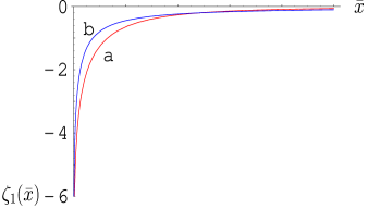
FIG. 1.: The ${\bar{x}}$-dependence of the vacuum polarization function $\zeta_{1}(\bar{x})$. Our result is described by (a) and the perturbative result is described by (b).

Notice that with (9) the (running) fine structure constant is expressed by

$$\bar{\alpha}({\bar{x}})=\displaystyle\frac{\alpha}{1+\displaystyle\frac{2\alpha}{\pi^{3}}\zeta_{1}({\bar{x}})},$$ (24)

where $\alpha$ is the asymptotic value of $\bar{\alpha}$ which we identify as $\alpha_{\infty}\simeq$ 1/137.036. This should be compared with well-known vacuum polarization function of perturbative QED [pesk]

$$\zeta_{1}({\bar{x}}) =-\pi^{2}\int_{0}^{1}dy~{}y(1-y)\ln{\Big{(}}1+\displaystyle\frac{\pi y(1-y)}{{\bar{x}}}{\Big{)}}$$ (26)

$$\simeq\displaystyle\frac{\pi^{2}}{6}~{}(~{}\ln\displaystyle\frac{{\bar{x}}}{\pi}+\displaystyle\frac{5}{3}~{}).~{}~{}~{}~{}~{}~{}~{}~{}~{}~{}({\bar{x}}\ll\pi)$$

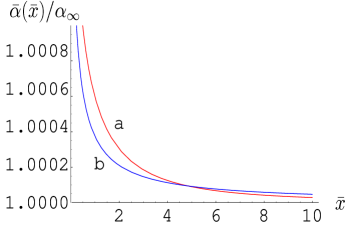
FIG. 2.: The ${\bar{x}}$-dependence of the fine structure constant $\bar{\alpha}(\bar{x})/\alpha_{\infty}$. Our result is described by (a), and the perturbative result is described by (b).

The vacuum polarization function $\zeta_{1}({\bar{x}})$ and the fine structure constant $\bar{\alpha}({\bar{x}})$ are plotted in Fig. 1 and Fig. 2. The contrast between our result and that of the perturbative QED is really remarkable. Obviously our result provides a significant modification to the perturbative result. Indeed we find $\bar{\alpha}({\bar{\mu}}=M_{z})\simeq$ 1/134.555 from our analysis, which should be compared with $\bar{\alpha}({\bar{\mu}}=M_{z})\simeq$ 1/134.647 of the perturbative QED. So we have about 0.07 % increase at $M_{z}\simeq$ 91.189 GeV. Notice that as the energy approaches to the ultra-violet limit the modification becomes larger. On the other hand in both cases we still have the Landau pole at a finite ${\bar{x}}$, although we can not see this clearly in the figure. We find that in our case the position of the Landau pole is given by ${\bar{x}}_{a}\simeq 17.7~{}{\rm x}~{}10^{-562}$, which is of the same order as the perturbative value ${\bar{x}}_{b}\simeq 7.4~{}{\rm x}~{}10^{-562}$. So the problem of the Landau pole in QED does not disappear with our non-perturbative correction.

From (9) we have the following $\beta$-function,

$$\beta({\bar{x}})={\bar{\mu}}\displaystyle\frac{d{\bar{e}}}{d{\bar{\mu}}}=\zeta_{2}({\bar{x}})~{}\bar{e}^{3},$$ (27)

where

$$\zeta_{2}({\bar{x}})=\displaystyle\frac{{\bar{x}}}{2\pi^{4}}\displaystyle\frac{d\zeta_{1}({\bar{x}})}{d{\bar{x}}}=\displaystyle\frac{{\bar{x}}^{3}}{4\pi^{4}}\displaystyle\frac{d^{3}f({\bar{x}})}{d{\bar{x}}^{3}}$$ (28)

$$=\displaystyle\frac{1}{12\pi^{2}}-\displaystyle\frac{{\bar{x}}^{2}}{4\pi^{4}}\sum_{n=1}^{\infty}\Big{[}1-n{\bar{x}}\Big{(}{\rm ci}(n{\bar{x}})\sin(n{\bar{x}})$$ (29)

$$-{\rm si}(n{\bar{x}})\cos(n{\bar{x}})\Big{)}\Big{]}.$$ (30)

On the other hand the perturbative QED gives

$$\zeta_{2}({\bar{x}})=\displaystyle\frac{1}{2\pi}\int_{0}^{1}dy~{}\displaystyle\frac{y^{2}(1-y)^{2}}{{\bar{x}}+\pi y(1-y)}.$$ (31)

The function $\zeta_{2}({\bar{x}})$ is plotted in Fig. 3.

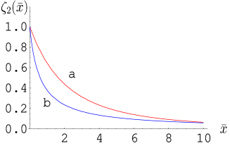
FIG. 3.: The ${\bar{x}}$-dependence of $\zeta_{2}({\bar{x}})$ which determines the $\beta$-function. Our result is given in (a) and the perturbative result is given in (b). Notice that they are normalized to one (in the unit $1/12\pi^{2}$) at the origin.

Notice that both our and perturbative $\zeta_{2}({\bar{x}})$ start from the same familiar value $\zeta_{2}(0)=1/12\pi^{2}$, but the discrepancy at a finite ${\bar{x}}$ is unmistakable.

Using (9) we can express the renormalized effective potential completely in terms of $\bar{\mu}$ and $\bar{e}$,

$$V_{\rm ren} = \displaystyle\frac{a^{2}}{2{\bar{e}}^{2}}\Big{(}1-\displaystyle\frac{{\bar{e}}^{2}}{2\pi^{4}}\zeta_{1}({\bar{x}})\Big{)}+\displaystyle\frac{a^{2}}{4\pi^{4}}f(x).$$ (32)

With this we obtain the Callan-Symanzik equation which guarantees the renormalization group invariance of the effective potential

$$\Big{(}\bar{\mu}\displaystyle\frac{\partial}{\partial\bar{\mu}}+\beta\displaystyle\frac{\partial}{\partial\bar{e}}\Big{)}V_{\rm ren}=0.$$ (33)

Notice that in our notation (3) we have absorbed the coupling constant $e$ to the gauge field, so that here we have no correction from the anomalous dimension of the gauge potential in the Callan-Symanzik equation.

The Callan-Symanzik equation implies that the effective potential (16) is independent of the scale parameter $\bar{x}$, so that one should be able to express the effective potential without the scale parameter. In fact with (11) we find

$$V_{\rm ren} = \displaystyle\frac{a^{2}}{2e_{\infty}^{2}}+\displaystyle\frac{a^{2}}{4\pi^{4}}f(x).$$ (34)

This tells that one can demonstrate the renormalization group invariance of the effective potential directly, without resorting to the Callan-Symanzik equation.

With this we have the renormalized effective action which has the manifest renormalization group invariance,

$${\cal L}_{\rm ren}=-\displaystyle\frac{a^{2}-b^{2}}{2e_{\infty}^{2}}-\displaystyle\frac{ab}{4\pi^{3}}\sum_{n=1}^{\infty}\displaystyle\frac{1}{n}{\Big{[}}\coth(\displaystyle\frac{n\pi b}{a})$$ (35)

$${\Big{(}}{\rm ci}(\displaystyle\frac{n\pi m^{2}}{a})\cos(\displaystyle\frac{n\pi m^{2}}{a})+{\rm si}(\displaystyle\frac{n\pi m^{2}}{a})\sin(\displaystyle\frac{n\pi m^{2}}{a}){\Big{)}}$$ (36)

$$-\displaystyle\frac{1}{2}\coth(\displaystyle\frac{n\pi a}{b}){\Big{(}}\exp(\displaystyle\frac{n\pi m^{2}}{b}){\rm Ei}(-\displaystyle\frac{n\pi m^{2}}{b})$$ (37)

$$+\exp(-\displaystyle\frac{n\pi m^{2}}{b}){\rm Ei}(\displaystyle\frac{n\pi m^{2}}{b}-i\epsilon){\Big{)}}{\Big{]}}.$$ (38)

Notice that the electric-magnetic duality of the effective action [1] remains intact under the above renormalization. The real and imaginary parts of the renormalized effective action are plotted in Fig. 4. In the region shown in the figures the quantum fluctuation provides about 0.1 % correction to the classical action.

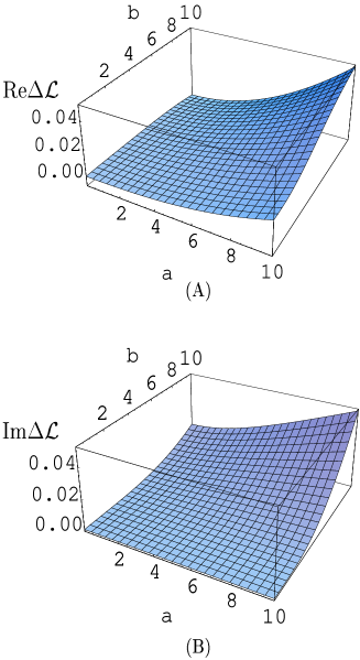
FIG. 4.: The one-loop correction to the dispersive part (A) and the absorptive part (B) of the effective action of QED (in the unit $m^{2}$).

One can obtain the similar results for the scalar QED. In this case in the pure magnetic and the pure electric background our one loop effective action reduces to [1]

$${\cal L}_{eff}=-\displaystyle\frac{a^{2}}{2e^{2}}{\Big{(}}1-\displaystyle\frac{e^{2}}{48\pi^{2}}\ln\displaystyle\frac{m^{2}}{\mu^{2}}{\Big{)}}$$ (39)

$$+\displaystyle\frac{a^{2}}{8\pi^{4}}\sum_{n=1}^{\infty}\displaystyle\frac{(-1)^{n}}{n^{2}}{\Big{(}}{\rm ci}(\displaystyle\frac{n\pi m^{2}}{a})\cos(\displaystyle\frac{n\pi m^{2}}{a})$$ (40)

$$+{\rm si}(\displaystyle\frac{n\pi m^{2}}{a})\sin(\displaystyle\frac{n\pi m^{2}}{a}){\Big{)}},$$ (41)

and

$${\cal L}_{eff}=\displaystyle\frac{b^{2}}{2e^{2}}{\Big{(}}1-\displaystyle\frac{e^{2}}{48\pi^{2}}\ln\displaystyle\frac{m^{2}}{\mu^{2}}{\Big{)}}$$ (42)

$$-\displaystyle\frac{b^{2}}{16\pi^{4}}\sum_{n=1}^{\infty}\displaystyle\frac{(-1)^{n}}{n^{2}}{\Big{(}}\exp(\displaystyle\frac{n\pi m^{2}}{b}){\rm Ei}(-\displaystyle\frac{n\pi m^{2}}{b})$$ (43)

$$+\exp(-\displaystyle\frac{n\pi m^{2}}{b}){\rm Ei}(\displaystyle\frac{n\pi m^{2}}{b}-i\epsilon){\Big{)}}.$$ (44)

So the effective potential in the pure magnetic background is given by

$$V_{eff}=\displaystyle\frac{a^{2}}{2e^{2}}{\Big{(}}1-\displaystyle\frac{e^{2}}{48\pi^{2}}\ln\displaystyle\frac{m^{2}}{\mu^{2}}{\Big{)}}+\displaystyle\frac{a^{2}}{8\pi^{4}}h(x),$$ (45)

$$h(x)=\displaystyle\frac{}{}\sum_{n=1}^{\infty}\displaystyle\frac{(-1)^{n}}{n^{2}}\Big{(}{\rm ci}(nx)\cos(nx)$$ (46)

$$+{\rm si}(nx)\sin(nx)\Big{)}.$$ (47)

From this with the definition (8) we find

$$\displaystyle\frac{1}{{\bar{e}}^{2}}=\displaystyle\frac{1}{e^{2}}{\Big{(}}1-\displaystyle\frac{e^{2}}{48\pi^{2}}\ln\displaystyle\frac{m^{2}}{\mu^{2}}{\Big{)}}+\displaystyle\frac{1}{4\pi^{4}}\eta_{1}({\bar{x}}),$$ (48)

$$\eta_{1}({\bar{x}})={\Big{(}}h(x)-x\displaystyle\frac{dh(x)}{dx}+\displaystyle\frac{x^{2}}{2}\displaystyle\frac{d^{2}h(x)}{dx^{2}}{\Big{)}}{\Big{|}}_{x={\bar{x}}}.$$ (49)

This gives us the following fine structure constant

$$\bar{\alpha}({\bar{x}})=\displaystyle\frac{\alpha}{1+\displaystyle\frac{\alpha}{\pi^{3}}\eta_{1}({\bar{x}})}.$$ (50)

With this we obtain the $\beta$-function for the scalar QED,

$$\beta(\bar{\mu})=\eta_{2}({\bar{x}})~{}\bar{e}^{3},$$ (51)

$$\eta_{2}({\bar{x}})=\displaystyle\frac{{\bar{x}}}{4\pi^{4}}\displaystyle\frac{d\eta_{1}}{d{\bar{x}}}=\displaystyle\frac{1}{48\pi^{2}}+\displaystyle\frac{{\bar{x}}^{2}}{8\pi^{4}}\sum_{n=1}^{\infty}(-1)^{n}\Big{[}1-n{\bar{x}}$$ (52)

$$\Big{(}{\rm ci}(n{\bar{x}})\sin(n{\bar{x}})-{\rm si}(n{\bar{x}})\cos(n{\bar{x}})\Big{)}\Big{]}.$$ (53)

From this we finally obtain the following renormalized effective action for the scalar QED,

$${\cal L}_{\rm ren}=-\displaystyle\frac{a^{2}-b^{2}}{2e_{\infty}^{2}}+\displaystyle\frac{ab}{8\pi^{3}}\sum_{n=1}^{\infty}\displaystyle\frac{(-1)^{n}}{n}{\Big{[}}{\rm csch}(\displaystyle\frac{n\pi b}{a})$$ (54)

$${\Big{(}}{\rm ci}(\displaystyle\frac{n\pi m^{2}}{a})\cos(\displaystyle\frac{n\pi m^{2}}{a})+{\rm si}(\displaystyle\frac{n\pi m^{2}}{a})\sin(\displaystyle\frac{n\pi m^{2}}{a}){\Big{)}}$$ (55)

$$-\displaystyle\frac{1}{2}{\rm csch}(\displaystyle\frac{n\pi a}{b}){\Big{(}}\exp(\displaystyle\frac{n\pi m^{2}}{b}){\rm Ei}(-\displaystyle\frac{n\pi m^{2}}{b})$$ (56)

$$+\exp(-\displaystyle\frac{n\pi m^{2}}{b}){\rm Ei}(\displaystyle\frac{n\pi m^{2}}{b}-i\epsilon){\Big{)}}{\Big{]}},$$ (57)

which is manifestly invariant under the renormalization group.

In this Letter we have presented a non-perturbative estimate of the vacuum polarization at an arbitrary scale, and demonstrated the renormalization group invariance of the one-loop effective action of QED. As far as we understand it, this is the first time that one has ever estimated the vacuum polarization non-perturbatively. The remarkale contrast between our result and the perturbative result is easy to understand theoretically. Compared to the perturbative one-loop estimate, our estimate includes infinitely more Feynman diagrams (one-loop diagrams with an arbitrary number of truncated photon legs). So, order by order, our estimate is better than the perturbative estimate. In this sense our estimate provides a definite improvement over the perturbative estimate.

Certainly one could try to compare our result with experiments. Here, however, we wish to emphasize the theoretical importance of our work. Our analysis provides a first non-perturbative estimate of the vacuum polarization in QED which is different from the existing perturbative estimate. This is really remarkable, because this is not always the case. In fact in QCD, one can show that the perturbative and non-perturbative estimates produce identical results, at least at one loop level [5].

Recently many interesting non-linear phenomena in electrodynamics (e.g., the reverse electromagnetic properties of matter, the superluminal propagation of light, the storage of light, etc.) have been studied experimentally [6]. Our result should become very useful in analyzing these non-linear effects of QED [7].

One of the authors (YMC) thanks Professor S. Adler, Professor F. Dyson, and Professor C. N. Yang for the illuminating discussions. The work is supported in part by Korea Research Foundation (KRF-2000-015-BP0072), and by the BK21 project of Ministry of Education.

REFERENCES

[1] Y. M. Cho and D. G. Pak, Phys. Rev. Lett.
86, 1947 (2001); W. S. Bae, Y. M. Cho, and D. G. Pak,
Phys. Rev. D64, 017303-1 (2001).
[2] W. Heisenberg and H. Euler, Z. Phys. 98 (1936) 714;
V. Weisskopf, Kgl. Danske Vid. Sel. Mat. Fys. Medd. 14, 6 (1936).
[3] J. Schwinger, Phys. Rev. 82 , 664 (1951).
[4] G. K. Savvidy, Phys. Lett. B71, 133 (1977).
[5] Y. M. Cho and D. G. Pak,
hep-th/0006051, submitted to Phys. Rev. D.
[6] D. Smith, W. Padilla, D. Vier, S. Nemat-Nasser, and S.
Schultz, Phys. Rev. Lett. 84, 4184 (2000);
L. Wang, A. Kuzmich, and A. Dogariu, Nature 406,
277 (2000); D. Phillips, A. Fleischhauer, A. Mair, R. Walsworth,
and M. Lukin, Phys. Rev. Lett. 86, 783 (2001).