hep-th/0007243

UTHEP-431

July, 2000

Duality Between String Junctions and D-Branes on Del Pezzo Surfaces

Kenji Mohri, Yukiko Ohtake and Sung-Kil Yang
Institute of Physics, University of Tsukuba
Ibaraki 305-8571, Japan

We revisit local mirror symmetry associated with del Pezzo surfaces in Calabi–Yau threefolds in view of five-dimensional ${\cal N}$=1 $E_{N}$ theories compactified on a circle. The mirror partner of singular Calabi–Yau with a shrinking del Pezzo four-cycle is described as the affine 7-brane backgrounds probed by a D3-brane. Evaluating the mirror map and the BPS central charge we relate junction charges to RR charges of D-branes wrapped on del Pezzo surfaces. This enables us to determine how the string junctions are mapped to D-branes on del Pezzo surfaces.

1 Introduction

Five-dimensional (5D) ${\cal N}$=1 theories with global exceptional symmetries are non-trivial interacting superconformal theories [1]. They appear in the strong-coupling limit of 5D ${\cal N}$=1 supersymmetric $SU(2)$ gauge theory with $N_{f}$ quark hypermultiplets. For $N_{f}\leq 8$ the microscopic global symmetry $SO(2N_{f})\times U(1)$ is enhanced to $E_{N_{f}+1}$. When $N_{f}=0$ we have two theories with global $E_{1}$ and $\widetilde{E}_{1}$ symmetry. The $\widetilde{E}_{1}$ theory is shown to further flow down to the $\widetilde{E}_{0}$ theory which has no global symmetry.

It is well-known that these 5D $E_{N}$ theories are obtained by compactifying M-theory on a Calabi–Yau threefold with a shrinking four-cycle realized by del Pezzo surfaces [2, 3]. Then the geometrical meaning of the sequence of $E$-type symmetries is most naturally understood in terms of the blowing-up process of $\boldsymbol{P}^{2}$ (or of $\boldsymbol{P}^{1}\times\boldsymbol{P}^{1}$) which yields del Pezzo surfaces. The correspondence is summarized in Table 1.

$\widetilde{E}_{0}$	$E_{1}$	$\widetilde{E}_{1}$, $E_{N}$ $(2\leq N\leq 8)$
$\boldsymbol{P}^{2}$	$\boldsymbol{P}^{1}\times\boldsymbol{P}^{1}$	$\boldsymbol{P}^{2}$ with the $N$ points blown up

Table 1: $E$-type symmetries and del Pezzo surfaces

Another interesting realization of 5D $E$-type theories is provided by the IIB 5-brane web construction including background 7-branes [4]. The advantageous point in this is that the affine property of $E_{N}$ symmetry, which has been known to occur naturally as the action of the Weyl group of the affine algebra $\widehat{E}_{N}$ in the study of the del Pezzo surfaces [5], can be captured explicitly by the 7-brane configurations, thanks to the recent advances in 7-brane technology [6, 7].

Furthermore it is shown that the Coulomb branch of 5D $E_{N}$ theories compactified on a circle is described in terms of a D3-brane probing the affine 7-brane backgrounds [8]. This provides us with an intuitive physical picture behind important calculations performed in [9, 10]. Then, in the light of the analysis of [9] and the 7-brane picture, we see that the $E_{N}$ theories on $\boldsymbol{R}^{4}\times S^{1}$ is considered as either the D3–7-brane system or the local system realized in singular Calabi–Yau space with a shrinking del Pezzo four-cycle; these two systems are mirror dual to each other. In this paper, thus, we revisit local mirror symmetry associated with del Pezzo surfaces in Calabi–Yau threefolds and elucidate on the relation between IIB string junctions in the affine 7-brane backgrounds and IIA D-branes wrapped on del Pezzo surfaces. A map between these two objects has been worked out recently in [11] in which an isomorphism between the junction lattices and the even homology lattice of del Pezzo surfaces, which is identified with the Ramond-Ramond (RR) charge lattice of IIA D-branes, is shown by comparing the intersection forms. In our approach, on the other hand, we evaluate explicitly the mirror map and the BPS central charge so as to convert junction charges to the central charges of D-branes.

The paper is organized as follows: In the next section, we calculate in detail the Seiberg–Witten (SW) period integrals which describe the Coulomb branch of 5D $E_{N}$ theories on $\boldsymbol{R}^{4}\times S^{1}$. The monodromy matrices and the prepotentials are obtained. In section 3, the mirror map is constructed. In section 4, we analyze D-branes localized on a surface. Several important invariants of the BPS D-branes such as the RR charge, the central charge and intersection pairings are given in algebro-geometrical terms. In section 5, the results of the preceding section are utilized to verify the map between string junctions and D-branes on a del Pezzo four-cycle.

2 Calculation of the periods and monodromies

The elliptic curves for the $\widehat{E}_{N}$ 7-brane configurations are obtained in [8, 12]. These curves describe the Coulomb branch of 5D $E_{N}$ theories compactified on $S^{1}$ [8]. For $E_{N=8,7,6}$ theories, they are given by [8, 9, 10]

$$\widehat{E}_{8} \quad:\quad y^{2}=x^{3}+R^{2}u^{2}x^{2}-2u^{5},$$

$$\widehat{E}_{7} \quad:\quad y^{2}=x^{3}+R^{2}u^{2}x^{2}+2u^{3}x,$$ (2.1)

$$\widehat{E}_{6} \quad:\quad y^{2}=x^{3}+R^{2}u^{2}x^{2}-2Riu^{3}x-u^{4},$$

where $u$ is a complex moduli parameter with mass dimension 6, 4, 3 for $\widehat{E}_{8}$, $\widehat{E}_{7}$, $\widehat{E}_{6}$ and $R$ is the radius of $S^{1}$. These curves have the discriminant

$$\widehat{E}_{8} \quad:\quad\Delta=-4u^{10}(2R^{6}u-27),$$

$$\widehat{E}_{7} \quad:\quad\Delta=-4u^{9}(R^{4}u-8),$$ (2.2)

$$\widehat{E}_{6} \quad:\quad\Delta=-iu^{8}(4R^{3}u+27i),$$

whose zeroes at $u=0$ represent coalescing $(N+2)$ 7-branes of $E_{N=8,7,6}$ configurations and a single zero at $u\neq 0$ represents a 7-brane which is responsible for extending $E_{N}$ to the affine system. The SW differentials $\lambda_{\text{SW}}$ associated with the $\widehat{E}_{N}$ curves are defined by

$$\frac{d\lambda_{\text{SW}}}{du}=\frac{dx}{y}+d(*),$$ (2.3)

which are known to take the logarithmic form [9, 10]. For the curves (2.1) we find

$$\widehat{E}_{8} \quad:\quad\lambda_{\text{SW}}=\frac{\kappa}{2\pi iR}\log\left(\frac{y-Rux}{y+Rux}\right)\frac{dx}{x},$$

$$\widehat{E}_{7} \quad:\quad\lambda_{\text{SW}}=\frac{\kappa}{2\pi iR}\log\left(\frac{y-Rux}{y+Rux}\right)\frac{dx}{x},$$ (2.4)

$$\widehat{E}_{6} \quad:\quad\lambda_{\text{SW}}=\frac{\kappa}{2\pi iR}\log\left(\frac{y-Rux+iu^{2}}{y+Rux-iu^{2}}\right)\frac{dx}{x-iu/R},$$

where $\kappa$ is a normalization constant and the factor $1/R$ ensures that $\lambda_{\text{SW}}$ has mass dimension unity. Notice that $\lambda_{\text{SW}}$ possesses the pole at $x=0$ for $\widehat{E}_{8}$, $\widehat{E}_{7}$ and $x=iu/R$ for $\widehat{E}_{6}$ because of the multivaluedness of the logarithm. Hence the set of period integrals $\Pi=(s,a,a_{D})$ consists of

$$s =\oint_{C}\lambda_{\text{SW}}=\frac{2\pi i\kappa}{R},$$ (2.5)

$$a(u) =\oint_{A}\lambda_{\text{SW}}=\int^{u}du^{\prime}\,\varpi(u^{\prime}),$$ (2.6)

$$a_{D}(u) =\oint_{B}\lambda_{\text{SW}}=\int^{u}du^{\prime}\,\varpi_{D}(u^{\prime}),$$ (2.7)

where the contour $C$ surrounds the pole of $\lambda_{\text{SW}}$ and $A$, $B$ are the homology cycles on $\widehat{E}_{N}$ torus along which the torus periods $\varpi(u)$, $\varpi_{D}(u)$ are defined as usual,

$$\varpi(u)=\oint_{A}\frac{dx}{y},\quad\varpi_{D}(u)=\oint_{B}\frac{dx}{y}.$$ (2.8)

2.1 Picard–Fuchs equations

The period $\Pi$ is evaluated with the use of the Picard–Fuchs equations. It is convenient to introduce a dimensionless variable

$$z=\frac{2}{27}R^{6}u,\quad\frac{1}{8}R^{4}u,\quad\frac{4i}{27}R^{3}u$$ (2.9)

for $\widehat{E}_{8}$, $\widehat{E}_{7}$, $\widehat{E}_{6}$, respectively, to write down the Picard–Fuchs equations. We obtain

$${\cal L}_{\widehat{E}_{N}}\Pi(z)=0,$$ (2.10)

where

$${\cal L}_{\widehat{E}_{8}} =\left[36z^{2}(z-1)\frac{d^{2}}{dz^{2}}+4z(27z-18)\frac{d}{dz}+(36z-5)\right]\frac{d}{dz},$$

$${\cal L}_{\widehat{E}_{7}} =\left[16z^{2}(z-1)\frac{d^{2}}{dz^{2}}+16z(3z-2)\frac{d}{dz}+(16z-3)\right]\frac{d}{dz},$$ (2.11)

$${\cal L}_{\widehat{E}_{6}} =\left[9z^{2}(z-1)\frac{d^{2}}{dz^{2}}+z(27z-18)\frac{d}{dz}+(9z-2)\right]\frac{d}{dz}.$$

In order to derive the solution we first solve the second-order equation for $d\Pi/dz$, and then integrate over $z$ to get $\Pi(z)$. Substituting the form $d\Pi/dz=z^{\rho}F(z)$ it is seen that $\rho=-\frac{5}{6}$, $-\frac{3}{4}$, $-\frac{2}{3}$ for $\widehat{E}_{8}$, $\widehat{E}_{7}$, $\widehat{E}_{6}$, and $F(z)$ obeys the standard hypergeometric equation

$$\left[z(1-z)\frac{d^{2}}{dz^{2}}+\left(\gamma-(\alpha+\beta+1)z\right)\frac{d}{dz}-\alpha\beta\right]F(z)=0,$$ (2.12)

with $\alpha=\beta=\rho+1$ and $\gamma=2(\rho+1)$, that is,

$$\alpha=\frac{1}{6},\quad\frac{1}{4},\quad\frac{1}{3}$$ (2.13)

for $\widehat{E}_{8},\widehat{E}_{7},\widehat{E}_{6}$. The torus periods around the regular singular points at $z=0,1,\infty$ are then expressed as

$$\begin{pmatrix}\varpi_{D}^{(\bullet)}(z)\\ \varpi^{(\bullet)}(z)\end{pmatrix}=C_{\bullet}\begin{pmatrix}\varphi_{1}^{(\bullet)}(z)\\ \varphi_{2}^{(\bullet)}(z)\end{pmatrix},$$ (2.14)

where $\bullet$ stands for $0,1,\infty$ corresponding to $z=0,1,\infty$, $C_{\bullet}$ are $2\times 2$ coefficient matrices and the set of fundamental solutions has been taken as follows:

$$\begin{cases}\varphi^{(0)}_{1}(z)=z^{-(1-\alpha)}{}_{2}F_{1}(\alpha,\alpha\,;2\alpha\,;z),\\ \varphi^{(0)}_{2}(z)=z^{-\alpha}{}_{2}F_{1}(1\!-\!\alpha,1\!-\!\alpha\,;2(1\!-\!\alpha)\,;\,z),\end{cases}$$ (2.15)

$$\begin{cases}\varphi^{(1)}_{1}(z)=z^{-(1-\alpha)}{}_{2}F_{1}(\alpha,\alpha\,;1\,;1\!-\!z),\\ \varphi^{(1)}_{2}(z)=z^{-(1-\alpha)}\left({}_{2}F_{1}(\alpha,\alpha,\,;1\,;1\!-\!z)\log(1\!-\!z)+{{}_{2}F_{1}}^{*}(\alpha,\alpha\,;1\,;1\!-\!z)\right),\end{cases}$$ (2.16)

and

$$\begin{cases}\varphi^{(\infty)}_{1}(z)=\frac{1}{z}\,{}_{2}F_{1}(\alpha,1\!-\!\alpha\,;1\,;\frac{1}{z}),\\ \varphi^{(\infty)}_{2}(z)=\frac{1}{z}\left({}_{2}F_{1}(\alpha,1\!-\!\alpha\,;1\,;\frac{1}{z})\log(-z)+{{}_{2}F_{1}}^{*}(\alpha,1\!-\!\alpha\,;1\,;\frac{1}{z})\right).\end{cases}$$ (2.17)

Here ${}_{2}F_{1}(\alpha,\beta\,;\gamma\,;z)$ is the hypergeometric function

$${}_{2}F_{1}(\alpha,\beta;\gamma;z)=\sum_{n=0}^{\infty}\frac{(\alpha)_{n}(\beta)_{n}}{(\gamma)_{n}}\frac{z^{n}}{n!}$$ (2.18)

and

$${{}_{2}F_{1}}^{*}(\alpha,\beta;\gamma;z)=\sum_{n=1}^{\infty}\frac{(\alpha)_{n}(\beta)_{n}}{(\gamma)_{n}}\left[\sum_{k=0}^{n-1}\left(\frac{1}{\alpha+k}+\frac{1}{\beta+k}-\frac{2}{\gamma+k}\right)\right]\frac{z^{n}}{n!},$$ (2.19)

where $(\alpha)_{n}=\Gamma(\alpha+n)/\Gamma(\alpha)$ with $\Gamma(x)$ being the gamma function.

The coefficient matrix $C_{1}$ is determined by directly evaluating the elliptic integrals. The result reads

$$C_{1}=\tilde{c}\,R^{\frac{1-\alpha}{\alpha}}\left(\begin{matrix}-\pi&0\\ \frac{i}{2}\left(\log v-i\pi\right)&-\frac{i}{2}\end{matrix}\right)$$ (2.20)

where $\tilde{c}=2^{2}/3^{3}$, $2^{-3/2}$, $2^{5/2}/3^{2}\,$ and

$$v=432,\quad 64,\quad 27$$ (2.21)

for $\widehat{E}_{8},\widehat{E}_{7},\widehat{E}_{6}$. Then, performing the analytic continuation we calculate $C_{0}$ and $C_{\infty}$. The connection matrices $X,Y$ defined by

$$\left(\begin{matrix}\varphi^{(0)}_{1}\\ \varphi^{(0)}_{2}\end{matrix}\right)=X\left(\begin{matrix}\varphi^{(1)}_{1}\\ \varphi^{(1)}_{2}\end{matrix}\right),\quad\left(\begin{matrix}\varphi^{(0)}_{1}\\ \varphi^{(0)}_{2}\end{matrix}\right)=Y\left(\begin{matrix}\varphi^{(\infty)}_{1}\\ \varphi^{(\infty)}_{2}\end{matrix}\right)$$ (2.22)

are found with the aid of the Barnes’ integral representation of the hypergeometric function [13, p. 286]. It turns out that

$$X=\left(\begin{matrix}\xi_{1}\eta_{1}&-\xi_{1}\\ \xi_{2}\eta_{2}&-\xi_{2}\end{matrix}\right),\quad Y=\left(\begin{matrix}\xi_{1}\eta_{1}\,e^{i\pi\alpha}&\xi_{1}\,e^{i\pi\alpha}\\ \xi_{2}\eta_{2}\,e^{i\pi(1-\alpha)}&\xi_{2}\,e^{i\pi(1-\alpha)}\end{matrix}\right),$$ (2.23)

where

$$\xi_{1}=\frac{\Gamma(2\alpha)}{\Gamma^{2}(\alpha)}, \quad\xi_{2}=\frac{\Gamma(2-2\alpha)}{\Gamma^{2}(1-\alpha)},$$ (2.24)

$$\eta_{1}=2(\psi(1)-\psi(\alpha)), \quad\eta_{2}=2(\psi(1)-\psi(1-\alpha)),$$ (2.25)

and $\psi(x)=\frac{d}{dx}\log\Gamma(x)$ is the digamma function. Thus we obtain

$$C_{0} =C_{1}X^{-1}=\frac{\pi R^{1-\alpha\over\alpha}}{2(2\alpha-1)}\left(\begin{matrix}2\xi_{2}&-2\xi_{1}\\ -\frac{\omega}{\sin\pi\alpha}\xi_{2}&\frac{\bar{\omega}}{\sin\pi\alpha}\xi_{1}\end{matrix}\right),\quad\omega=e^{i\pi\left(\frac{1}{2}-\alpha\right)},$$ (2.26)

$$C_{\infty} =C_{1}X^{-1}Y=R^{1-\alpha\over\alpha}\left(\begin{matrix}-(\log v+i\pi)\sin\pi\alpha&-\sin\pi\alpha\\ \frac{i\pi}{2\sin\pi\alpha}&0\end{matrix}\right).$$ (2.27)

When the periods go around each regular singular point counterclockwise they undergo the monodromy. If we denote as $T_{\bullet}$ the monodromy matrix of $\left(\begin{matrix}\varphi_{1}^{(\bullet)}\\ \varphi_{2}^{(\bullet)}\end{matrix}\right)$, the monodromy matrix $\hat{M}_{\bullet}$ acting on $\left(\begin{matrix}\varpi_{D}^{(\bullet)}\\ \varpi^{(\bullet)}\end{matrix}\right)$ is given by $\hat{M}_{\bullet}=C_{\bullet}T_{\bullet}C_{\bullet}^{-1}$. For $\widehat{E}_{N=8,7,6}$ one computes

$$\hat{M}_{0}=\left(\begin{matrix}N-8&N-9\\ 1&1\end{matrix}\right),\quad\hat{M}_{1}=\left(\begin{matrix}1&0\\ -1&1\end{matrix}\right),\quad\hat{M}_{\infty}=\left(\begin{matrix}1&N-9\\ 0&1\end{matrix}\right)$$ (2.28)

which obey $\hat{M}_{\infty}=\hat{M}_{0}\hat{M}_{1}$, $\hat{M}_{0}^{6}={1}$ ($\widehat{E}_{8}$), $\hat{M}_{0}^{4}={1}$ ($\widehat{E}_{7}$), $\hat{M}_{0}^{3}={1}$ ($\widehat{E}_{6}$). If we follow the convention in [7], $K_{\bullet}=\hat{M}_{\bullet}^{-1}$ yields the monodromy around the 7-brane configurations. For the $[p,q]$ 7-brane $\boldsymbol{X}_{[p,q]}$, the monodromy matrix reads [7]

$$K_{[p,q]}=\left(\begin{matrix}1+pq&-p^{2}\\ q^{2}&1-pq\end{matrix}\right),$$ (2.29)

whereas for the $\widehat{E}_{N}$ 7-branes we have

$$K(\boldsymbol{\hat{E}}_{N})=\left(\begin{matrix}1&9-N\\ 0&1\end{matrix}\right).$$ (2.30)

In (2.28) we observe $\hat{M}_{\infty}^{-1}=K(\boldsymbol{\hat{E}}_{N})$, $\hat{M}_{1}^{-1}=K_{[0,1]}$ and $\hat{M}_{0}^{-1}=K_{[3,-2]}K_{[3,-1]}K_{[1,0]}^{N}$. Accordingly our 7-brane configuration is identified as

$$\boldsymbol{\hat{E}}_{N}=\boldsymbol{A}^{N}\boldsymbol{X}_{[3,-1]}\boldsymbol{X}_{[3,-2]}\boldsymbol{X}_{[0,1]},$$ (2.31)

where we have used the notation in [7] and $\boldsymbol{A}=\boldsymbol{X}_{[1,0]}$ is the D7-brane. This is shown to be equivalent to the canonical one $\boldsymbol{\hat{E}}_{N}=\boldsymbol{A}^{N-1}\boldsymbol{B}\boldsymbol{C}^{2}\boldsymbol{X}_{[3,1]}$ by making use of the brane move [14].

2.2 Seiberg–Witten periods

Now our task is to calculate the Seiberg–Witten periods $a(z)$, $a_{D}(z)$ from the torus periods through (2.5)–(2.7). The important subtlety arises in evaluating the integration constants. First of all, since $\lambda_{\text{SW}}$ vanishes at $u=0$, $a(z)$ and $a_{D}(z)$ must vanish as well at $z=0$ [9]. In the patch $|z|<1$, the SW periods are thus given by

$$a_{D}^{(0)}(z) =\int_{0}^{z}dz^{\prime}\,\varpi_{D}^{(0)}(z^{\prime}),$$ (2.32)

$$a^{(0)}(z) =\int_{0}^{z}dz^{\prime}\,\varpi^{(0)}(z^{\prime}).$$ (2.33)

We note that these are succinctly expressed in terms of the generalized hypergeometric function

$${}_{3}F_{2}(\alpha_{1},\alpha_{2},\alpha_{3};\beta_{1},\beta_{2};z)=\sum_{n=0}^{\infty}\frac{(\alpha_{1})_{n}(\alpha_{2})_{n}(\alpha_{3})_{n}}{(\beta_{1})_{n}(\beta_{2})_{n}}\frac{z^{n}}{n!}$$ (2.34)

in such a way that

$$\left(\begin{matrix}a_{D}^{(0)}(z)\\ a^{(0)}(z)\end{matrix}\right)=C_{0}\left(\begin{matrix}V_{1}^{(0)}(z)\\ V_{2}^{(0)}(z)\end{matrix}\right),$$ (2.35)

where

$$V_{1}^{(0)}(z) =\frac{1}{\alpha}\,z^{\alpha}\,{}_{3}F_{2}(\alpha,\alpha,\alpha\,;2\alpha,1\!+\!\alpha\,;z),$$ (2.36)

$$V_{2}^{(0)}(z) =\frac{1}{1-\alpha}\,z^{1-\alpha}\,{}_{3}F_{2}(1\!-\!\alpha,1\!-\!\alpha,1\!-\!\alpha\,;2(1\!-\!\alpha),2\!-\!\alpha;z).$$ (2.37)

Next the SW periods in the patch $|1-z|\leq 1$ are

$$a_{D}^{(1)}(z) =\int_{1}^{z}dz^{\prime}\,\varpi_{D}^{(1)}(z^{\prime})+c_{D}^{(1)},$$ (2.38)

$$a^{(1)}(z) =\int_{1}^{z}dz^{\prime}\,\varpi^{(1)}(z^{\prime})+c^{(1)},$$ (2.39)

where $c_{D}^{(1)}$ and $c^{(1)}$ are integration constants. Notice that the analytic continuation allows us to write

$$a_{D}^{(1)}(z)=\int_{0}^{z}dz^{\prime}\,\varpi_{D}^{(1)}(z^{\prime})$$ (2.40)

which obeys $a_{D}^{(1)}(0)=a_{D}^{(0)}(0)=0$. Therefore,

$$c_{D}^{(1)} =a_{D}^{(1)}(1)$$

$$=-\pi\int_{0}^{1}dx\,x^{-(1-\alpha)}{}_{2}F_{1}(\alpha,\alpha;1;1-x)$$

$$=-\pi\sum_{n=0}^{\infty}\frac{(\alpha)_{n}^{2}}{n!}\frac{\Gamma(\alpha)}{\Gamma(\alpha+n+1)}$$

$$=-\pi\frac{\Gamma(\alpha)}{\Gamma(\alpha+1)}\,{}_{2}F_{1}(\alpha,\alpha;1+\alpha;1).$$ (2.41)

Here the well-known formula

$${}_{2}F_{1}(\alpha,\beta;\gamma;1)=\frac{\Gamma(\gamma)\Gamma(\gamma-\alpha-\beta)}{\Gamma(\gamma-\alpha)\Gamma(\gamma-\beta)},\quad\mbox{Re}\,\gamma>0,\quad\mbox{Re}(\gamma-\alpha-\beta)>0$$ (2.42)

helps us to find

$$c_{D}^{(1)}=-\pi\Gamma(\alpha)\Gamma(1-\alpha)=-\frac{\pi^{2}}{\sin\pi\alpha}.$$ (2.43)

Since $c_{D}^{(1)}$ is also obtained from $c_{D}^{(1)}=a_{D}^{(0)}(1)$, (2.43) yields the nontrivial identity for the generalized hypergeometric function ${}_{3}F_{2}$ at $z=1$ via (2.35). For $\alpha=\frac{1}{3}$, this identity was first found numerically in [15], for which the above calculation affords analytic proof.

On the other hand, the similar integral for $a^{(1)}(1)$ is not helpful to determine $c^{(1)}$ analytically. Hence, evaluating $c^{(1)}=a^{(0)}(1)$ numerically we determine

$$c^{(1)}=\frac{\pi^{2}}{\sin\pi\alpha}\times\begin{cases}0.5000+0.9281i\quad\mbox{for}\;\widehat{E}_{8}\\ 0.5000+0.6103i\quad\mbox{for}\;\widehat{E}_{7}\\ 0.5000+0.4628i\quad\mbox{for}\;\widehat{E}_{6}.\end{cases}$$ (2.44)

These constants were first evaluated in [16, 17].

Let us now turn to the analysis of the SW periods around $z=\infty$. In order to fix the integration constants, we adopt the idea in [18] and employ the Barnes’ integral representation of the hypergeometric function

$${}_{2}F_{1}(\alpha,\beta;\gamma;z)=\frac{\Gamma(\gamma)}{\Gamma(\alpha)\Gamma(\beta)}\int_{-i\infty}^{i\infty}\frac{dt}{2\pi i}\frac{\Gamma(t+\alpha)\Gamma(t+\beta)\Gamma(-t)}{\Gamma(t+\gamma)}(-z)^{t},$$ (2.45)

where $|\arg(-z)|<\pi$. When the integration contour is closed on the right we have the power series as presented in (2.15) which converges for $|z|<1$. For our purpose, we first check how (2.45) can be used to reproduce the SW periods in the patch $|z|<1$. The naive idea is that expressing the torus periods in the form (2.45), we first make the $z$-integral and then perform the contour integral with respect to $t$. We are thus led to consider the integral

$$I_{\alpha}(z)=\frac{\Gamma(2\alpha)}{\Gamma^{2}(\alpha)}\int_{-i\infty}^{i\infty}\frac{dt}{2\pi i}\frac{\Gamma^{2}(t+\alpha)\Gamma(-t)}{\Gamma(t+1-\alpha)(t+\alpha)}(-z)^{t}z^{\alpha}.$$ (2.46)

Closing the contour on the right we immediately obtain

$$I_{\alpha}(z)_{\text{right}}=\frac{1}{\alpha}z^{\alpha}\,{}_{3}F_{2}(\alpha,\alpha,\alpha;2\alpha,1+\alpha;z),$$ (2.47)

and hence (2.35) is reproduced.

If we close the contour on the left, we obtain the expression which is valid for $|z|>1$. Thus

$$\left(\begin{matrix}a_{D}^{(\infty)}(z)\\ a^{(\infty)}(z)\end{matrix}\right)=C_{0}\left(\begin{matrix}I_{\alpha}(z)_{\text{left}}\\ I_{1-\alpha}(z)_{\text{left}}\end{matrix}\right).$$ (2.48)

Upon doing the contour integral on the left, one has to pick up the triple pole at $t=-\alpha$ in addition to the standard poles in the Barnes’ integral. This in fact gives rise to the integration constant. After some algebra we arrive at

$$\left(\begin{matrix}a_{D}^{(\infty)}(z)\\ a^{(\infty)}(z)\end{matrix}\right)=C_{\infty}\left(\begin{matrix}V_{1}^{(\infty)}(z)\\ V_{2}^{(\infty)}(z)\end{matrix}\right)+C_{0}\left(\begin{matrix}b_{1}\\ b_{2}\end{matrix}\right),$$ (2.49)

where

$$V_{1}^{(\infty)}(z) =\log(-z)-g(z),$$ (2.50)

$$V_{2}^{(\infty)}(z) =\frac{1}{2}\log^{2}(-z)-\log(-z)g(z)+h(z),$$ (2.51)

with

$$g(z) =\sum_{n=1}^{\infty}\frac{(\alpha)_{n}(1-\alpha)_{n}}{(n!)^{2}n}\frac{1}{z^{n}},$$ (2.52)

$$h(z) =\sum_{n=1}^{\infty}\frac{(\alpha)_{n}(1-\alpha)_{n}}{(n!)^{2}n}\left[\sum_{k=0}^{n-1}\left(\frac{1}{\alpha+k}+\frac{1}{1-\alpha+k}-\frac{2}{1+k}\right)-\frac{1}{n}\right]\frac{1}{z^{n}}.$$ (2.53)

In (2.49) the integration constants read

$$b_{1}=\frac{1}{2}e^{i\pi\alpha}\xi_{1}\left(\eta_{1}^{2}+\frac{\pi^{2}}{3}\right),\quad b_{2}=\frac{1}{2}e^{i\pi(1-\alpha)}\xi_{2}\left(\eta_{2}^{2}+\frac{\pi^{2}}{3}\right).$$ (2.54)

Further manipulations yield

$$a_{D}^{(\infty)}(z)=-4\pi^{2}\sin\pi\alpha\,\frac{H_{2}(z)}{(2\pi i)^{2}},\quad a^{(\infty)}(z)=\frac{\pi^{2}}{\sin\pi\alpha}\frac{H_{1}(z)}{2\pi i},$$ (2.55)

where

$$H_{1}(z) =-\log(-vz)+g(z),$$ (2.56)

$$H_{2}(z) =-\frac{1}{2}\log^{2}(vz)+\log(vz)g(z)-h(z)-\frac{\pi^{2}}{2}\left(\frac{1}{\sin^{2}\pi\alpha}+\frac{1}{3}\right).$$ (2.57)

Now that we have fixed all the integration constants, it is seen that the monodromy matrices with integral entries are obtained by setting the constant period

$$s=\frac{\pi^{2}}{\sin\pi\alpha}.$$ (2.58)

As a result, the monodromy matrices acting on the period vector ${}^{t}\Pi={}^{t}(s,a(z),a_{D}(z))$ for $\widehat{E}_{N=8,7,6}$ theories turn out to be

$$M_{0}=\begin{pmatrix}1&0&0\\ 0&1&1\\ 0&N-9&N-8\end{pmatrix},\quad M_{1}=\begin{pmatrix}1&0&0\\ -1&1&-1\\ 0&0&1\end{pmatrix},\quad M_{\infty}=\begin{pmatrix}1&0&0\\ -1&1&0\\ 9-N&N-9&1\end{pmatrix}$$

which obey $M_{\infty}=M_{0}M_{1}$, $M_{0}^{6}={1}$ ($\widehat{E}_{8}$), $M_{0}^{4}={1}$ ($\widehat{E}_{7}$) and $M_{0}^{3}={1}$ ($\widehat{E}_{6}$).

Finally the BPS central charge is expressed in terms of the period integrals

$$Z=pa(z)-qa_{D}(z)+ns,$$ (2.60)

where $(p,q)\in\boldsymbol{Z}^{2}$ are electric and magnetic charges and $n\in\boldsymbol{Z}$ is global conserved charge of the BPS states. In view of the D3-probe picture, (2.60) is the central charge corresponding to the string junction,

$$\boldsymbol{J}=\sum_{i=1}^{N}\lambda_{i}\boldsymbol{\omega}^{i}+P\,\boldsymbol{\omega}^{p}+Q\,\boldsymbol{\omega}^{q}-n\,\boldsymbol{z}_{[0,1]},$$ (2.61)

where $P=p$, $Q=q+n$ and our notation is as follows; $\{\lambda_{i}\}$ is the Dynkin label of $E_{N}$ weights and the $\boldsymbol{\omega}^{i}$ are the junctions of zero asymptotic charges representing the fundamental weights of the Lie algebra $E_{N}$, $\boldsymbol{\omega}^{p}$, $\boldsymbol{\omega}^{q}$ are the $E_{N}$ singlet junctions with asymptotic charges $(1,0)$, $(0,1)$, respectively, and $\boldsymbol{z}_{[0,1]}$ stands for the outgoing (0,1)-string emanating from the 7-brane $\boldsymbol{X}_{[0,1]}$ at $z=1$. See Fig. 1a for the $\widehat{E}_{N}$ brane-junction configurations probed by a single D3-brane. To justify the above correspondence, for instance, take a junction with charges $(p,q\,;n)=(0,-1;1)$. This is a single BPS string stretched between the D3-brane and the 7-brane $\boldsymbol{X}_{[0,1]}$. Clearly its mass vanishes when the D3-brane is located at the point $z=1$. This is indeed verified from (2.60) since $Z(z)=a_{D}(z)+s$ for $(0,-1;1)$ charges and $Z(1)=a_{D}(1)+s=0$ at $z=1$ by virtue of (2.43).

We note that there are no terms in (2.60) which reflect the presence of the $E_{N}$ non-singlet junctions in (2.61) explicitly. To have such terms one has to turn on mass deformation parameters in the $\widehat{E}_{N}$ curves so that the SW differentials have poles with non-vanishing residues other than the one at $x=0$ ($x=iu/R$ for $\widehat{E}_{6}$). This will produce additional terms in (2.60) which may depend directly on the $E_{N}$ representations.

Notice that the string junction (2.61) is equivalently expressed as

$$\boldsymbol{J}=\sum_{i=1}^{N}\lambda_{i}\boldsymbol{\omega}^{i}+p\,\boldsymbol{\omega}^{p}+q\,\boldsymbol{\omega}^{q}+n\,\boldsymbol{\delta}^{(-1,0)},$$ (2.62)

where $\boldsymbol{\delta}^{(-1,0)}$ is a loop junction which represents the imaginary root of the affine algebra $\widehat{E}_{N}$, see Fig. 1b. In the junction realization of $\widehat{E}_{N}$, the level $k$ of representations is given by $k(\boldsymbol{J})=-(\boldsymbol{J},\boldsymbol{\delta}^{(-1,0)})=-q$, while the grade $\bar{n}(\lambda)$ for a weight vector $\{\lambda_{i}\}$ is equal to $n$ in $\boldsymbol{J}$ up to a constant shift [7].

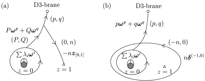
Figure 1: String junctions on the $\widehat{E}_{N}$ 7-brane configuration

On the D3-brane probing the region $|z|<1$, in the limit $R\rightarrow 0$, the theory reduces to the 4D superconformal theory with global exceptional symmetries [19, 20]. Recovering the $R$-dependence we have the central charge in the form

$$Z=pa(u)-qa_{D}(u)+\frac{n}{R}s,$$ (2.63)

where $a(u)$, $a_{D}(u)\simeq\mbox{const}\cdot u^{\alpha}$ and the last term represents the KK modes associated with the $S^{1}$ compactification. We thus observe that the grading of KK modes is regarded as the the grade in the affine symmetry $\widehat{E}_{N}$. As will be seen in section 5.3 these KK modes are identified with the D0-branes in M-theory. The decoupling of the KK modes as $R\rightarrow 0$ is ensured since the 7-brane $\boldsymbol{X}_{[0,1]}$ moves away to infinity on the $u$-plane, and hence the loop junction $\boldsymbol{\delta}^{(-1,0)}$ decouples, leaving the finite symmetry $E_{N}$ for 4D theories.

3 Mirror map

5D ${\cal N}$=1 supersymmetric $SU(2)$ gauge theories with exceptional global symmetries [1] are realized by compactifying M-theory on a Calabi–Yau threefold with a vanishing del Pezzo four-cycle [2, 3]. In [9] the local mirror geometry of the singularity associated with a shrinking del Pezzo four-cycle of the type $E_{N=8,7,6}$ is modeled by the Landau-Ginzburg potential

$$W_{E_{8}} =\frac{1}{x_{0}^{6}}+x_{1}^{2}+x_{2}^{3}+x_{3}^{6}+x_{4}^{6}-\psi x_{0}x_{1}x_{2}x_{3}x_{4},$$

$$W_{E_{7}} =\frac{1}{x_{0}^{4}}+x_{1}^{2}+x_{2}^{4}+x_{3}^{4}+x_{4}^{4}-\psi x_{0}x_{1}x_{2}x_{3}x_{4},$$ (3.1)

$$W_{E_{6}} =\frac{1}{x_{0}^{3}}+x_{1}^{3}+x_{2}^{3}+x_{3}^{3}+x_{4}^{3}-\psi x_{0}x_{1}x_{2}x_{3}x_{4}.$$

The equations $W_{E_{N}}=0$ describe non-compact Calabi–Yau manifolds and $\psi$ is a complex moduli parameter. The point $\psi=0$ is the $E_{N}$ symmetric point (the Landau-Ginzburg point) at which the del Pezzo four-cycle collapses. The large complex structure limit is taken by letting $\psi=\infty$.

It turns out that the natural complex modulus is $\psi^{\ell}$ with $\ell=6$ ($E_{8}$), 4 ($E_{7}$) and 3 ($E_{6}$) and, as will be seen momentarily, $\psi^{\ell}$ and $z$ in the previous section is related through

$$z=\frac{\psi^{6}}{432}\;(E_{8}),\quad\frac{\psi^{4}}{64}\;(E_{7}),\quad\frac{\psi^{3}}{27}\;(E_{6}).$$ (3.2)

The period integral $\widetilde{\Pi}$ of the holomorphic three-form $\Omega$ associated with (3.1) are defined over a basis of three-cycles on the mirror Calabi–Yau ​​​. They obey the Picard–Fuchs equations [9]

$${\cal L}_{\text{ell}}^{E_{N}}\cdot\vartheta\,\widetilde{\Pi}=0,$$ (3.3)

where $\vartheta=c\frac{\partial}{\partial c}$ with $c=\psi^{-\ell}$ and ${\cal L}_{\text{ell}}^{E_{N}}$ are the Picard–Fuchs operators corresponding to the elliptic singularities of type $\widehat{E}_{N}$

$${\cal L}_{\text{ell}}^{E_{8}} =\vartheta^{2}-12c(6\vartheta+5)(6\vartheta+1),$$

$${\cal L}_{\text{ell}}^{E_{7}} =\vartheta^{2}-4c(4\vartheta+3)(4\vartheta+1),$$ (3.4)

$${\cal L}_{\text{ell}}^{E_{6}} =\vartheta^{2}-3c(3\vartheta+2)(3\vartheta+1).$$

Making a change of variables with (3.2), one can check that (3.3) is equivalent to (2.11). In fact, it is shown in [9] that the Calabi–Yau periods $\widetilde{\Pi}(c)$ over three-cycles reduce to the SW periods $\Pi$ after performing the integrals over appropriate two-cycles. Thus we have $\widetilde{\Pi}=\Pi=(s,a(z),a_{D}(z))$.

Under mirror symmetry three-cycles on the IIB side is mapped to the zero, two, four-cycles on the IIA side where the four-cycle is the del Pezzo surface. Following the standard machinery [21] we find that the complex Kähler modulus $t$ is given by

$$t(z)=\frac{H_{1}(z)}{2\pi i}$$ (3.5)

and its dual $t_{d}$ becomes

$$t_{d}(z)=\frac{\partial{\cal F}}{\partial t}=-\frac{H_{2}(z)}{(2\pi i)^{2}}.$$ (3.6)

Thus the SW periods and the flat coordinate system are related via

$$\left(\begin{matrix}s\\ a(z)\\ a_{D}(z)\end{matrix}\right)=\frac{\pi^{2}}{\sin\pi\alpha}\left(\begin{matrix}1&0&0\\ 0&1&0\\ 0&0&4\sin^{2}\pi\alpha\end{matrix}\right)\left(\begin{matrix}1\\ t(z)\\ t_{d}(z)\end{matrix}\right).$$ (3.7)

The central charge (2.60) is then rewritten as

$$Z=\frac{\pi^{2}}{\sin\pi\alpha}\left(-4\sin^{2}\pi\alpha\,q\,t_{d}(z)+p\,t(z)+n\right).$$ (3.8)

In the large radius region $|z|>1$, it is shown from (2.55) that

$$t_{d}=\frac{t^{2}}{2}-\frac{t}{2}-\frac{1}{24}\left(\frac{3}{\sin^{2}\pi\alpha}-2\right)+O(e^{2\pi it}),$$ (3.9)

from which we see that $t_{d}$ is the central charge of the D4-brane. Integrating this over $t$ we obtain the prepotential

$${\cal F}=\frac{t^{3}}{6}-\frac{t^{2}}{4}-\frac{1}{24}\left(\frac{3}{\sin^{2}\pi\alpha}-2\right)t+\mbox{const.}-\frac{1}{(2\pi i)^{3}}\sum_{k=1}^{\infty}n_{k}Li_{3}(e^{2\pi ikt}),$$ (3.10)

where $Li_{3}(x)$ is the trilogarithm and the instanton coefficients $n_{k}$ are presented in Table 2. We note that the $n_{k}$’s multiplied by $4\sin^{2}\pi\alpha$ for $\widehat{E}_{N}$ coincide with the Gromov–Witten invariants obtained in [22].

	$\widehat{E}_{8}$	$\widehat{E}_{7}$	$\widehat{E}_{6}$
$n_{1}$	$252$	$28$	$9$
$n_{2}$	$-9252$	$-136$	$-18$
$n_{3}$	$848628$	$1620$	$81$
$n_{4}$	$-114265008$	$-29216$	$-576$
$n_{5}$	$18958064400$	$651920$	$5085$
$n_{6}$	$-3589587111852$	$-16627608$	$-51192$
$n_{7}$	$744530011302420$	$465215604$	$565362$
$n_{8}$	$-165076694998001856$	$-13927814272$	$-6684480$
$n_{9}$	$38512679141944848024$	$439084931544$	$83246697$
$n_{10}$	$-9353163584375938364400$	$-14417814260960$	$-1080036450$

Table 2: Instanton coefficients

4 D-branes on a surface

The aim of this section is to obtain several basic invariants of BPS D-branes bounded on a surface, which are expressed as coherent sheaves on the surface, such as the RR charge, the central charge, and some intersection pairings with the aid of some algebraic geometry techniques. They play a crucial role in the duality map between D-branes on del Pezzo surfaces and the string junctions with $\widehat{E}_{N}$ symmetry, which we will discuss in the next section. An important note is that though we identify a BPS D-brane on a surface with a coherent sheaf, we do not enter into the conditions, such as the stability, to be satisfied by the sheaf to represent a true BPS brane, with few exceptions; in effect, what we really need is not a sheaf itself but its invariants such as the Chern character in this article.

4.1 D-branes on a Calabi–Yau threefold

We represent a BPS D-brane on a Calabi–Yau threefold $X$ by a coherent ${\cal O}_{X}$-module ${\cal G}$. The RR charge of ${\cal G}$ is given by the Mukai vector [23, 24]

$$v_{X}\left({\cal G}\right)={\text{ch}}\left({\cal G}\right)\sqrt{{\text{Todd}}\left(T_{X}\right)}\in H_{2\bullet}(X;\boldsymbol{Q}):=\bigoplus_{i=0}^{3}H_{2i}\left(X;\boldsymbol{Q}\right),$$ (4.1)

where ${\text{ch}}({\cal G})=\sum_{i=0}^{3}{\text{ch}}_{i}({\cal G})$ is the Chern character with ${\text{ch}}_{i}({\cal G})\in H_{6-2i}(X;\boldsymbol{Q})$, which can be computed as follows: there always exits a resolution of ${\cal G}$ by locally free sheaves $(V_{\bullet})$, that is, sheaves of sections of holomorphic vector bundles: $0\to V_{3}\to V_{2}\to V_{1}\to V_{0}\to{\cal G}\to 0$ (exact), thus we can set ${\text{ch}}({\cal G})\colon=\sum_{i=0}^{3}\,(-1)^{i}\,{\text{ch}}(V_{i})$, which does not depend on the choice of the resolution, and $\sqrt{{\text{Todd}}(T_{X})}=[X]+c_{2}(X)/24$, the effect of which on the RR charges has been called a geometric version of the Witten effect in [24].

The intersection form on D-branes on $X$, which is of great importance in investigating topological aspects of D-branes [25, 26], is given by

$$I_{X}\left({\cal G}_{1},{\cal G}_{2}\right)=\big{\langle}v_{X}({\cal G}_{1})^{\vee}\cdot v_{X}({\cal G}_{2})\big{\rangle}_{X}=\big{\langle}{\text{ch}}\left({\cal G}_{1}\right)^{\vee}\cdot{\text{ch}}\left({\cal G}_{2}\right)\cdot{\text{Todd}}\left(T_{X}\right)\big{\rangle}_{X},$$ (4.2)

where $\langle\cdots\rangle_{X}$ evaluates the degree of $H_{0}\left(X;\boldsymbol{Q}\right)\cong\boldsymbol{Q}$ component, and $v\rightarrow v^{\vee}$ flips the sign of $H_{0}(X)\oplus H_{4}(X)$ part. In particular, if ${\cal G}$ itself is locally free, then ${\text{ch}}({\cal G})^{\vee}={\text{ch}}({\cal G}^{\vee})$, where ${\cal G}^{\vee}={\cal H}om_{X}({\cal G},{\cal O}_{X})$ is the dual sheaf.

It is easy to check $I_{X}({\cal G}_{2},{\cal G}_{1})=-I_{X}({\cal G}_{1},{\cal G}_{2})$. On the other hand, the Hirzebruch–Riemann–Roch formula [27, 28] tells us

$$I_{X}\left({\cal G}_{1},{\cal G}_{2}\right)=\sum_{i=0}^{3}\,(-1)^{i}\,{\text{dim}}\,{\text{Ext}}^{i}_{X}({\cal G}_{1},{\cal G}_{2}),$$ (4.3)

according to which the skew-symmetric property of the intersection form $I_{X}$ may be attributed to the Serre duality: ${\text{Ext}}_{X}^{i}({\cal G}_{2},{\cal G}_{1})\cong{\text{Ext}}_{X}^{3-i}({\cal G}_{1},{\cal G}_{2})^{\vee}$ [29]. Incidentally, the H.R.R. formula (4.3) also assures that $I_{X}$ takes values in $\boldsymbol{Z}$.

Let $J_{X}\in H_{4}(X;\boldsymbol{R})$ be a Kähler form on $X$, which is identified with an $\boldsymbol{R}$-extended ample divisor here. The classical expression of the central charge of the D-brane ${\cal G}$ is then given by [25, 26]

$$Z_{J_{X}}^{\text{cl}}({\cal G})=-\big{\langle}e^{-J_{X}}\cdot v_{X}({\cal G})\big{\rangle}_{X}=-\sum_{k=0}^{3}\frac{(-1)^{k}}{k!}\big{\langle}J^{k}_{X}\cdot v_{X,k}({\cal G})\big{\rangle}_{X},$$ (4.4)

where $v_{X,k}$ is the $H_{2k}(X)$ component of $v_{X}\in H_{2\bullet}(X)$. On the other hand, the quantum central charge $Z_{J_{X}}({\cal G})$ differs from its classical counterpart (4.4) by the terms of order $O(e^{-2\pi\langle J_{X}\cdot\beta\rangle_{X}})$ where two-cycle $\beta$ is in the Mori cone of $X$, which is dual to the Kähler cone; the exact Kähler moduli dependence of $Z_{J_{X}}$ can be determined in principle by the Picard–Fuchs equations for the periods of the mirror Calabi–Yau threefold $X^{\vee}$ [30, 15, 31].

4.2 D-branes localized on a surface

Let $f\colon S\,{\hookrightarrow}\,X$ be an embedding of a projective surface $S$ in a Calabi–Yau threefold $X$. If $c_{1}(S)\in H_{2}(S)$ is nef, which means that its intersection with any effective curve $C$ on $S$ are non-negative: $c_{1}(S)\cdot C\geq 0$, there is a smooth elliptic Calabi–Yau threefold over $S$ with $S$ its cross section, which we can take as a model of embedding [32]. Other examples of embedding can be found in [9, 24, 33, 34].

Now let us take the limit of infinite elliptic fiber, so that the D-branes the central charge of which remains finite are those which are confined to the surface $S$, where we should note that some D-branes on $S$, a D0-brane for example, can move along elliptic fibers so as to leave $S$ even if $S$ itself is rigid in $X$. The properties of the D-branes localized on $S$ then depend not on the details of the global model $X$, but only on the intrinsic geometry of $S$ and its normal bundle $N_{S}=N_{S|X}$, which is isomorphic to the canonical line bundle $K_{S}$. In particular, this means that we can compute the central charges of BPS D-branes using local mirror symmetry principle on $S$ [32].

A D-brane sticking to $S$ can be described by a coherent ${\cal O}_{S}$-module ${\cal E}$. The Euler number of it defined by $\chi({\cal E})=\sum_{i=0}^{2}\,(-1)^{i}\,h^{i}(S,{\cal E})$, where $h^{i}(S,{\cal E})={\text{dim}}\,H^{i}(S,{\cal E})$, is an important invariant, which can be obtained as follows: first we need the Todd class of $S$

$${\text{Todd}}(T_{S}) =[S]+\frac{1}{2}\,c_{1}(S)+\chi({\cal O}_{S})\,[{\text{pt}}],$$ (4.5)

$$\chi({\cal O}_{S}) =\frac{1}{12}\big{\langle}c_{2}(S)+c_{1}(S)^{2}\big{\rangle}_{S},$$ (4.6)

second, by the H.R.R. formula, we have

$$\chi({\cal E})=\big{\langle}{\text{ch}}({\cal E})\,{\text{Todd}}(T_{S})\big{\rangle}_{S}=r\,\chi({\cal O}_{S})+\big{\langle}{\text{ch}}_{2}({\cal E})+\frac{1}{2}\,c_{1}(S)\cdot c_{1}({\cal E})\big{\rangle}_{S}.$$ (4.7)

There is a canonical push-forward homomorphism $f_{*}\colon H_{2\bullet}(S;\boldsymbol{Q})\,{\rightarrow}\,H_{2\bullet}(X;\boldsymbol{Q})$, which maps a cycle on $S$ to that on $X$. Similarly, we can define the coherent sheaf $f_{!}\,{\cal E}$ on $X$ by extending ${\cal E}$ by zero to $X\backslash S$. The celebrated Grothendieck–Riemann–Roch formula [27, 35] for embedding $f\colon S\,{\hookrightarrow}\,X$ relates the Chern characters of ${\cal E}$ and $f_{!}\,{\cal E}$ as follows:

$${\text{ch}}(f_{!}\,{\cal E})=f_{*}\left({\text{ch}}({\cal E})\,\frac{1}{{\text{Todd}}(N_{S})}\right).$$ (4.8)

Multiplying the both hand side of (4.8) by the square root of ${\text{Todd}}(T_{X})$, we have

$${\text{ch}}(f_{!}\,{\cal E})\sqrt{{\text{Todd}}(T_{X})}=f_{*}\left({\text{ch}}({\cal E})\sqrt{\frac{{\text{Todd}}(T_{S})}{{\text{Todd}}(N_{S})}}\right),$$ (4.9)

where we have used the projection formula [36, p. 273], [37, p. 426]:

$$f_{*}\left(\alpha\cdot\!f^{*}\beta\right)=f_{*}\alpha\cdot\!\beta,\qquad\alpha\in H_{2\bullet}(S;\boldsymbol{Q}),\quad\beta\in H_{2\bullet}(X;\boldsymbol{Q}),$$ (4.10)

and $f^{*}{\text{Todd}}(T_{X})={\text{Todd}}(T_{S})\cdot{\text{Todd}}(N_{S})$, which follows from the short exact sequence of bundles on $S$: $0\rightarrow T_{S}\rightarrow f^{*}T_{X}\rightarrow N_{S}\rightarrow 0,$ combined with the multiplicative property of the Todd class. As the left hand side of (4.9) is the D-brane charge of ${\cal E}$ regarded as a brane on $X$, we arrive at the intrinsic description of the RR charge on $S$:

$$v_{S}({\cal E})={\text{ch}}({\cal E})\sqrt{\frac{{\text{Todd}}(T_{S})}{{\text{Todd}}(K_{S})}}={\text{ch}}({\cal E})\,e^{\frac{1}{2}c_{1}(S)}\,\sqrt{\frac{\widehat{A}(T_{S})}{\widehat{A}(K_{S})}}\in H_{2\bullet}(S;\boldsymbol{Q}),$$ (4.11)

which is a complex-analytic (or algebraic) derivation of the RR charge which has originally been obtained in $C^{(\infty)}$ category [38, 39]. The gravitational correction factor for $S$ admits the following expansion:

$$\sqrt{\frac{{\text{Todd}}(T_{S})}{{\text{Todd}}(K_{S})}}=[S]+\frac{1}{2}c_{1}(S)+\frac{1}{24}\big{(}c_{2}(S)+3c_{1}(S)^{2}\big{)}\in H_{2\bullet}(S;\boldsymbol{Q}).$$ (4.12)

As a simple exercise let us compute the RR charge of a sheaf on $S$. To this end, let $\iota\colon C\hookrightarrow S$ be an embedding of a smooth genus $g$ curve in $S$ with normal bundle $N_{C}=N_{C|S}$. Then from a line bundle $L_{C}$ on $C$, we obtain a torsion sheaf $\iota_{!}L_{C}$ on $S$. ${\text{ch}}(\iota_{!}\,L_{C})$ can be computed again from the G.R.R. formula:

$${\text{ch}}(\iota_{!}\,L_{C})=\iota_{*}\left({\text{ch}}(L_{C})\,\frac{1}{{\text{Todd}}(N_{C})}\right)=\iota_{*}[C]+\big{(}\deg(L_{C})-\frac{1}{2}\deg(N_{C})\big{)}[{\text{pt}}],$$ (4.13)

where $\deg(L):=\langle c_{1}(L)\rangle_{C}$ for a line bundle $L$ on $C$. The RR charge of the torsion ${\cal O}_{S}$-module $\iota_{!}\,L_{C}$ can then be computed as

$$v_{S}(\iota_{!}\,L_{C})=\iota_{*}[C]+\chi(L_{C})[{\text{pt}}]\in H_{2}(S)\oplus H_{0}(S),$$ (4.14)

where we have used the classical adjunction and the self-intersection formulae on $S$:

$$2g(C)-2 =\big{\langle}[C]\cdot[C]-[C]\cdot c_{1}(S)\big{\rangle}_{S},$$ (4.15)

$$\deg(N_{C}) =\big{\langle}[C]\cdot[C]\big{\rangle}_{S},$$ (4.16)

as well as the classical Riemann–Roch formula on $C$:

$$\chi(L_{C})=h^{0}(C,L_{C})-h^{1}(C,L_{C})=\deg(L_{C})+1-g.$$ (4.17)

Let us next turn to intersection pairings on D-branes. It seems that the most appropriate intersection form on D-branes on $S$ could depend on one’s purpose. Below, we will describe three candidates, each of which we think has its own reason to be chosen as an intersection form.

The first uses the Mukai vector $v_{S}$ (4.11) and defines a symmetric form:

$$I_{S}({\cal E}_{1},{\cal E}_{2}) =-\big{\langle}v_{S}({\cal E}_{1})^{\vee}\cdot v_{S}({\cal E}_{2})\big{\rangle}_{S}$$

$$=\frac{1}{12}\,r_{1}r_{2}\,\chi(S)+\big{\langle}r_{1}\,{\text{ch}}_{2}({\cal E}_{2})+r_{2}\,{\text{ch}}_{2}({\cal E}_{1})-c_{1}({\cal E}_{1})\cdot c_{1}({\cal E}_{2})\big{\rangle}_{S},$$ (4.18)

where ${\text{ch}}({\cal E})=r[S]+c_{1}({\cal E})+{\text{ch}}_{2}({\cal E})$, $\chi(S)=\langle c_{2}(S)\rangle_{S}$ the Euler number of $S$, and $v^{\vee}=-v_{0}+v_{1}-v_{2}$ [23, 28], with $v_{i}$ being the $H_{2i}(S)$ component of $v$. It should also be noted that $I_{S}$ is not $\boldsymbol{Z}$-valued in general.

The second is the skew-symmetric form $I_{X}\text{\small$\circ$}f_{!}$ induced from the one on the ambient Calabi–Yau threefold $X$ (4.2). As shown below, however, this form has an description intrinsic to $S$ independent of the details of embedding:

$$I_{X}(f_{!}\,{\cal E}_{1},f_{!}\,{\cal E}_{2}) =\big{\langle}f_{*}(v_{S}({\cal E}_{1}))^{\vee}\cdot f_{*}(v_{S}({\cal E}_{2}))\big{\rangle}_{X}$$

$$=\big{\langle}r_{1}\,c_{1}({\cal E}_{2})\cdot c_{1}(S)-r_{2}\,c_{1}({\cal E}_{1})\cdot c_{1}(S)\big{\rangle}_{S},$$ (4.19)

where we have used the self-intersection formula: $f^{*}f_{*}[S]=c_{1}(N_{S})$ [37, p. 431], as well as the projection formula (4.10) to show that for $[S]\in H_{4}(S)$, $[C]\in H_{2}(S;\boldsymbol{Q})$

$$f_{*}[S]\cdot f_{*}[C]=f_{*}\big{(}[C]\cdot f^{*}f_{*}[S]\big{)}=-f_{*}\big{(}[C]\cdot c_{1}(S)\big{)}.$$ (4.20)

To be explicit, consider $S=\boldsymbol{P}^{2}$. $H_{2}(\boldsymbol{P}^{2})$ is isomorphic to $\boldsymbol{Z}$, the ample generator of which we denote by $l$. Then $c_{1}(\boldsymbol{P}^{2})=3l$, and $\langle l\cdot l\rangle_{\boldsymbol{P}^{2}}=1$. Following Diaconescu and Gomis [40], we express the Chern character of a coherent sheaf ${\cal E}$ on $\boldsymbol{P}^{2}$ as

$$r({\cal E})=-n_{2},\quad c_{1}({\cal E})=n_{1}l,\quad{\text{ch}}_{2}({\cal E})=-n_{0}[{\text{pt}}],$$ (4.21)

where $n_{1},n_{2}\in\boldsymbol{Z}$, and $n_{0}\in\frac{1}{2}n_{1}+\boldsymbol{Z}$. Our second intersection form can be written in these variables as follows:

$$I_{X}(f_{!}\,{\cal E},f_{!}\,{\cal E}^{\prime})=-3(n_{1}^{\prime}n_{2}-n_{1}n_{2}^{\prime}),$$ (4.22)

which is precisely the intersection form in [40] up to sign. An interesting remark is that the intersection form (4.22) introduced in [40] is based on that of one-cycles on an $\widehat{E}_{6}$ torus contained in $\boldsymbol{P}^{2}$, while our $I_{X}\text{\small$\circ$}f_{!}$ is induced from that on a Calabi–Yau threefold $X$ which contains $\boldsymbol{P}^{2}$.

The third, which has been used in [11] to identify the RR charge lattice $H_{2\bullet}(S)$ with $S$ a del Pezzo surface and the string junction charge lattices, generalizing the result in [4], would be the most natural one also from the mathematical point of view [28, 23]:

$$\chi_{S}({\cal E}_{1},{\cal E}_{2}) =\sum_{i=0}^{2}(-1)^{i}\dim{\text{Ext}}_{S}^{i}({\cal E}_{1},{\cal E}_{2})$$

$$=-\big{\langle}{\text{ch}}({\cal E}_{1})^{\vee}\cdot{\text{ch}}({\cal E}_{2})\cdot{\text{Todd}}(T_{S})\big{\rangle}_{S}$$

$$=r_{1}r_{2}\,\chi({\cal O}_{S})+\big{\langle}r_{1}\,{\text{ch}}_{2}({\cal E}_{2})+r_{2}\,{\text{ch}}_{2}({\cal E}_{1})-c_{1}({\cal E}_{1})\cdot c_{1}({\cal E}_{2})\big{\rangle}_{S}$$

$$+\frac{1}{2}\,\big{\langle}r_{1}\,c_{1}({\cal E}_{2})\cdot c_{1}(S)-r_{2}\,c_{1}({\cal E}_{1})\cdot c_{1}(S)\big{\rangle}_{S}.$$ (4.23)

The skew-symmetric part of the third form $\chi_{S}$ coincides with $I_{X}\text{\small$\circ$}f_{!}$:

$$\chi_{S}({\cal E}_{1},{\cal E}_{2})-\chi_{S}({\cal E}_{2},{\cal E}_{1})=I_{X}(f_{!}\,{\cal E}_{1},f_{!}\,{\cal E}_{2}),$$ (4.24)

while the relation between the symmetric part of $\chi_{S}$ and $I_{S}$ becomes

$$\frac{1}{2}\big{(}\chi_{S}({\cal E}_{1},{\cal E}_{2})+\chi_{S}({\cal E}_{2},{\cal E}_{1})\big{)}=\frac{1}{12}\,r_{1}r_{2}\left\langle c_{1}(S)^{2}\right\rangle_{S}+I_{S}({\cal E}_{1},{\cal E}_{2}).$$ (4.25)

In view of the Serre duality: ${\text{Ext}}_{S}^{i}({\cal E}_{1},{\cal E}_{2})\cong{\text{Ext}}_{S}^{2-i}({\cal E}_{2},{\cal E}_{1}\otimes K_{S})^{\vee}$, the skew-symmetric part of $\chi_{S}$ (4.24) comes from the non-triviality of the canonical line bundle $K_{S}$.

According to the Bogomolov inequality, the discriminant of a sheaf ${\cal E}$, defined by

$$\Delta({\cal E}):=\big{\langle}-2r\,{\text{ch}}_{2}({\cal E})+c_{1}({\cal E})^{2}\big{\rangle}_{S},$$

must be non-negative if ${\cal E}$ is torsion-freeand semi-stable [28], which puts the following constraint on the self-intersection number of a torsion-free ${\cal O}_{S}$-module ${\cal E}$ corresponding to a true BPS D-brane:

$$\chi_{S}({\cal E},{\cal E})=r^{2}\,\chi({\cal O}_{S})-\Delta({\cal E})\leq r^{2}\,\chi({\cal O}_{S}).$$ (4.26)

Let $J_{S}\in H_{2}(S;\boldsymbol{R})$ be a Kähler class on $S$. The classical central charge of ${\cal E}$ measured by $J_{S}$ then admits an expression intrinsic to $S$:

$$Z_{J_{S}}^{\text{cl}}({\cal E})=-\big{\langle}e^{-J_{S}}\cdot v_{S}({\cal E})\big{\rangle}_{S}.$$ (4.27)

In particular, if $J_{S}$ is obtained as a restriction of a Kähler class $J_{X}$ on $X$, then (4.27) coincides with $Z_{J_{X}}^{\text{cl}}(f_{!}\,{\cal E})$: the central charge measured on $X$ by $J_{X}$.

5 String junctions versus del Pezzo surfaces

5.1 del Pezzo surfaces

A del Pezzo surface is a surface the first Chern class of which is ample. Apart from $\widetilde{B}_{1}\!=\!\boldsymbol{P}^{1}\times\boldsymbol{P}^{1}$, they are obtained by blowing up generic $N$ points on $\boldsymbol{P}^{2}$ for $0\leq N\leq 8$, which we call ${B}_{N}$ in this article. Our main interest is of course in the three cases $N\!=\!8,7,6$. The homology groups of ${B}_{N}$ are

$$H_{2\bullet}\left({B}_{N}\right)=\boldsymbol{Z}\,[{B}_{N}]\oplus\boldsymbol{Z}\,l\oplus\boldsymbol{Z}\,e_{1}\oplus\cdots\oplus\boldsymbol{Z}\,e_{N}\oplus\boldsymbol{Z}\,[{\text{pt}}],$$ (5.1)

where $l$ represents the pull-back of a line of $\boldsymbol{P}^{2}$, and $e_{1},\dots,e_{N}$ the exceptional divisors, by which the first Chern class is written as $c_{1}({B}_{N})=3l-\sum_{i=1}^{N}e_{i}$. We also note that the Picard group of ${B}_{N}$ is isomorphic to $H_{2}({B}_{N})$, which means that each element of $H_{2}({B}_{N})$ is realized as the first Chern class of a holomorphic line bundle on ${B}_{N}$ which is unique up to isomorphism. Intersection pairings on $H_{2}({B}_{N})$ are given by

$$\langle l\cdot l\rangle_{{B}_{N}}=1,\quad\langle l\cdot e_{i}\rangle_{{B}_{N}}=0,\quad\langle e_{i}\cdot e_{j}\rangle_{{B}_{N}}=-\delta_{i,j}.$$ (5.2)

We list here some topological invariants:

$$\big{\langle}c_{1}({B}_{N})^{2}\big{\rangle}_{{B}_{N}}=9-N,\quad\big{\langle}c_{2}({B}_{N})\big{\rangle}_{{B}_{N}}=3+N,\quad\chi({\cal O}_{{B}_{N}})=1.$$ (5.3)

The gravitational correction factor in the Mukai vector (4.12) is given by

$$\sqrt{\frac{{\text{Todd}}(T_{{B}_{N}})}{{\text{Todd}}(K_{{B}_{N}})}}=[{B}_{N}]+\frac{1}{2}\,c_{1}({B}_{N})+\frac{1}{12}(15-N)[{\text{pt}}]\in H_{2\bullet}({B}_{N};\boldsymbol{Q}).$$ (5.4)

The degree of $[C]\in H_{2}({B}_{N};\boldsymbol{Q})$ is defined by ${d}([C])=\langle[C]\cdot c_{1}({B}_{N})\rangle_{{B}_{N}}$. If we expand it as $[C]=a_{0}\,l+\sum_{i=1}^{N}a_{i}\,e_{i}$, then we see ${d}([C])=3a_{0}+\sum_{i=1}^{N}a_{i}$. It is also convenient to associate the following two quantities to a coherent ${\cal O}_{{B}_{N}}$-module ${\cal E}$: let $d({{\cal E}})$ be the degree of $c_{1}({\cal E})$, and $k({{\cal E}})=\langle{\text{ch}}_{2}({\cal E})\rangle_{{B}_{N}}$, in terms of which the Euler number of ${\cal E}$ (4.7) can be expressed as

$$\chi({\cal E})=h^{0}(S,{\cal E})-h^{1}(S,{\cal E})+h^{2}(S,{\cal E})=r({\cal E})+\frac{1}{2}d({\cal E})+k({\cal E}).$$ (5.5)

It is known that the degree zero sublattice of $H_{2}({B}_{N})$ is isomorphic to the $E_{N}$ root lattice, the root system of which is composed of the self-intersection $-2$ elements. For $3\leq N\leq 8$, the $N$ simple roots can be chosen as

$$\boldsymbol{\alpha}_{i}=e_{i}-e_{i+1},\ 1\leq i<N,\qquad\boldsymbol{\alpha}_{N}=l-e_{1}-e_{2}-e_{3}.$$ (5.6)

The fundamental weight $\boldsymbol{w}^{i}\in H_{2}({B}_{N};\boldsymbol{Q})$ is uniquely determined by $\langle\boldsymbol{w}^{i}\cdot\boldsymbol{\alpha}_{j}\rangle_{{B}_{N}}=-\delta_{j}^{i}$, and $d({\boldsymbol{w}^{i}})=0$. Any $[C]\in H_{2}({B}_{N})$ then admits the following orthogonal decomposition into the degree and the $E_{N}$ weight:

$$[C]=\frac{{d}([C])}{9-N}\,c_{1}({B}_{N})+\sum_{i=1}^{N}\lambda_{i}([C])\,\boldsymbol{w}^{i},$$ (5.7)

where the Dynkin labels are determined by $\lambda_{i}([C])\!=\!-\langle[C]\cdot\boldsymbol{\alpha}_{i}\rangle_{{B}_{N}}$; for a coherent sheaf ${\cal E}$, its Dynkin labels $\lambda_{i}({\cal E})$ can be defined in the same way using $c_{1}({\cal E})\in H_{2}({B}_{N})$, that is,

$$c_{1}({\cal E})=\frac{d({\cal E})}{9-N}\,c_{1}({B}_{N})+\sum_{i=1}^{N}\lambda_{i}({\cal E})\,\boldsymbol{w}^{i}.$$ (5.8)

The third intersection form $\chi_{N}:=\chi_{{B}_{N}}$ (4.23) can then be expressed as

$$\chi_{N}({\cal E}_{1},{\cal E}_{2})=r_{1}\,r_{2}+r_{1}\,k_{2}+r_{2}\,k_{1}+\lambda_{1}\cdot\lambda_{2}-\frac{d_{1}\,d_{2}}{9-N}+\frac{1}{2}\,\left(r_{1}\,d_{2}-r_{2}\,d_{1}\right).$$ (5.9)

For more information on del Pezzo surfaces see, for example, [10, 4, 11, 2, 3, 41].

${B}_{N}$ has a natural one-parameter family of complexified Kähler classes $J_{S}=t\,c_{1}({B}_{N})$, with ${\text{Im}}(t)\!>\!0$, because $c_{1}({B}_{N})$ is an ample divisor. The degree of a curve defined above is nothing but the volume of it measured by the normalized Kähler class $J_{S}=c_{1}({B}_{N})$.

Using (4.11) combined with (5.4), it is now straightforward to compute the classical central charge of a D-brane ${\cal E}$ measured by the Kähler class $J_{S}=t\,c_{1}({B}_{N})$:

$$Z_{t}^{\text{cl}}({\cal E}) =-\big{\langle}e^{-tc_{1}({B}_{N})}v_{{B}_{N}}({\cal E})\big{\rangle}_{{B}_{N}}$$

$$=-r({\cal E})\,(9-N)\left(\frac{t^{2}}{2}-\frac{t}{2}+\frac{1}{12}\,\frac{3-N}{9-N}\right)+d({\cal E})\,t-\chi({\cal E}).$$ (5.10)

Recall that the exact quantum central charge $Z({\cal E})$ yields the classical one evaluated above (5.10) modulo the instanton correction terms $O(e^{2\pi it})$. In particular, for the cases $N=8,7,6$, the instanton expansion of the central charge (3.9) of the D4-brane obtained in the previous section takes the form:

$$t_{d}=\left(\frac{t^{2}}{2}-\frac{t}{2}+\frac{1}{12}\,\frac{3-N}{9-N}\right)+O(e^{2\pi it}),$$ (5.11)

in writing which we have noticed that $4\sin^{2}\pi\alpha=9-N$ for $\widehat{E}_{N=8,7,6}$. The classical part of $t_{d}$ coincides with the one in (5.10). Therefore we can make the following identification of the quantum central charge of the D-brane ${\cal E}$ measured by the Kähler form $tc_{1}({B}_{N})$ by

$$Z_{t}({\cal E})=-r({\cal E})\,(9-N)\,t_{d}+d({\cal E})\,t-\chi({\cal E}).$$ (5.12)

We are now in a position to compare the two central charges of the one and the same $\widehat{E}_{N}$ theory; one obtained by the analysis of the SW periods (2.60), and the other by the geometric method (5.12). They are related under mirror symmetry through (3.8) so that we have the following dictionary between the charges, after a trivial rescaling of the former:

$$p =d({\cal E}),$$

$$q =r({\cal E}),$$ (5.13)

$$-n =\chi({\cal E})=r({\cal E})+\frac{1}{2}d({\cal E})+k({\cal E}).$$

In passing, we give a comment on the $N\!=\!0$ case. Upon a change of variables: $t=\frac{1}{3}t_{b}+\frac{1}{2}$, where the constant shift implies the existence of the NS B-field flux on $\boldsymbol{P}^{2}$ [40], (5.10) becomes

$$Z^{\text{cl}}({\cal E})=-\left\langle e^{-t_{b}l}{\text{ch}}({\cal E})\sqrt{\frac{\widehat{A}(T_{\boldsymbol{P}^{2}})}{\widehat{A}(N_{\boldsymbol{P}^{2}})}}\right\rangle_{\boldsymbol{P}^{2}}=-r({\cal E})\,\left(\frac{t_{b}^{2}}{2}+\frac{1}{8}\right)+\frac{1}{3}d({\cal E})\,t_{b}-k({\cal E}),$$ (5.14)

where $l$ is the ample generator of divisors. This is precisely the classical central charge on $\boldsymbol{P}^{2}$ treated as the $\boldsymbol{Z}_{3}$ orbifold in [40, 42, 43].

5.2 $\boldsymbol{E}_{\bf 9}$ almost del Pezzo surface

An $E_{9}$ almost del Pezzo surface ${B}_{9}$ is a surface obtained by blowing up nine points of $\boldsymbol{P}^{2}$ which are the complete intersection of two cubics on $\boldsymbol{P}^{2}$. It has the structure of elliptic fibration $\pi\colon{B}_{9}\to\boldsymbol{P}^{1}$, which has twelve degenerate fibers leaving the total space non-singular for a generic choice of parameters, which we assume throughout the paper. As its name stands for, ${B}_{9}$ shares many properties with the del Pezzo surfaces ${B}_{N}$; to be explicit, among the formulae in the preceding subsection, (5.1)–(5.5) remain valid for ${B}_{9}$ if one simply sets $N\!=\!9$ there, as well as the definition of the first Chern class $c_{1}({B}_{9})$. It is then clear that the elements of $H_{2}({B}_{9})$ orthogonal to both $c_{1}({B}_{9})$ and $e_{9}$ generate the $E_{8}$ root lattice. Let $[{\text{F}}]$ and $[{\text{B}}]$ be the class of $H_{2}({B}_{9})$ defined by the fiber and a cross section of the fibration respectively. We can then make the following identification:

$$[{\text{F}}]=c_{1}({B}_{9})=3l-\sum_{i=1}^{9}e_{i},\quad[{\text{B}}]=e_{9},$$ (5.15)

the intersection pairings of which we give here for convenience:

$$\big{\langle}[{\text{F}}]\cdot[{\text{F}}]\big{\rangle}_{{B}_{9}}=0,\quad\big{\langle}[{\text{F}}]\cdot[{\text{B}}]\big{\rangle}_{{B}_{9}}=1,\quad\big{\langle}[{\text{B}}]\cdot[{\text{B}}]\big{\rangle}_{{B}_{9}}=-1.$$ (5.16)

As opposed to the case of del Pezzo surfaces, $c_{1}({B}_{9})$ is no longer an ample divisor; it is only a nef divisor with self-intersection zero, so that $c_{1}({B}_{9})$ alone cannot define a Kähler class on ${B}_{9}$. However, the structure of elliptic fibration suggests the following natural two-parameter family of the complexified Kähler classes on ${B}_{9}$:

$$J=t_{1}[{\text{F}}]+t_{2}\left([{\text{F}}]+[{\text{B}}]\right)=(t_{1}+t_{2})\,c_{1}({B}_{9})+t_{2}\,e_{9},$$ (5.17)

where the imaginary parts of $t_{1}$ and $t_{2}$ parametrize the volume of the curve $[{\text{B}}]$ and $[{\text{F}}]$ measured by ${\text{Im}}\,(J)$ respectively, which span the Kähler sub-cone of our model. A serious treatment of the stability condition of coherent ${\cal O}_{{B}_{9}}$-modules would face with the problem of subdivision of the Kähler cone, because the stability condition depends on the choice of Kähler class ${\text{Im}}\,(J)$ [44], which we will not discuss further in this article. By the way, another two-parameter family of Kähler classes $\tilde{J}$ treated in [34] can be written in our notation as $\tilde{J}=\tilde{t}_{1}\,[{\text{F}}]+\tilde{t}_{2}\,l$.

The classical central charge of the D-brane represented by a coherent ${\cal O}_{{B}_{9}}$-module ${\cal E}$ can be computed as:

$$Z^{\text{cl}}({\cal E}) =-\left\langle e^{-t_{1}[{\text{F}}]-t_{2}([{\text{F}}]+[{\text{B}}])}\cdot{\text{ch}}({\cal E})\cdot\big{(}[{B}_{9}]+\frac{1}{2}[{\text{F}}]+\frac{1}{2}[{\text{pt}}]\big{)}\right\rangle_{{B}_{9}}$$

$$=-r({\cal E})\left(\frac{t_{2}^{2}}{2}+t_{1}t_{2}-\frac{t_{2}}{2}-\frac{1}{2}\right)+d({\cal E})\,(t_{1}+t_{2})+b({\cal E})\,t_{2}-\chi({\cal E}),$$ (5.18)

where $d({\cal E})$ and $b({\cal E})$ are the two integers defined by the decomposition of $c_{1}({\cal E})$:

$$c_{1}({\cal E})=b({\cal E})\,[{\text{F}}]+d({\cal E})\,([{\text{B}}]+[{\text{F}}])+\sum_{i=1}^{8}\lambda_{i}({\cal E})\,\boldsymbol{w}^{i}.$$ (5.19)

That is, they are obtained via $b({\cal E})=\langle[{\text{B}}]\cdot c_{1}({\cal E})\rangle_{{B}_{9}}$, $d({\cal E})=\langle[{\text{F}}]\cdot c_{1}({\cal E})\rangle_{{B}_{9}}$. In terms of these variables, the intersection form $\chi_{9}:=\chi_{{B}_{9}}$ can be written as

$$\chi_{9}({\cal E}_{1},{\cal E}_{2})=r_{1}\,r_{2}+r_{1}\,k_{2}+r_{2}\,k_{1}-d_{1}\,d_{2}-b_{1}\,d_{2}-b_{2}\,d_{1}+\lambda_{1}\cdot\lambda_{2}+\frac{1}{2}(r_{1}\,d_{2}-r_{2}\,d_{1}).$$ (5.20)

A period $\varpi$ obeys the Picard–Fuchs differential equations: ${\cal L}^{(1)}\varpi=0,\ {\cal L}^{(2)}\varpi=0,$ with

$${\cal L}^{(1)} =\big{(}\vartheta_{1}-z_{1}\left(\vartheta_{1}-\vartheta_{2}\right)\big{)}\,\vartheta_{1},$$ (5.21)

$${\cal L}^{(2)} =\vartheta_{2}\left(\vartheta_{2}-\vartheta_{1}\right)-z_{2}(\vartheta_{2}+\tfrac{1}{6})(\vartheta_{2}+\tfrac{5}{6}),$$ (5.22)

which can be obtained from the standard procedure of the local mirror principle [32] using a realization of ${B}_{9}$ as a hypersurface in a toric threefold. It is easy to see that we can take the two periods of the $\widehat{E}_{8}$ torus:

$$\varpi_{0}(z_{2})={}_{2}F_{1}\big{(}\tfrac{1}{6},\tfrac{5}{6};1;z_{2}\big{)},\quad\varpi^{(2)}_{1}(z_{2})=\frac{1}{2\pi i}\,\big{(}\varpi_{0}(z_{2})\log(\frac{z_{2}}{432})+{{}_{2}F_{1}}^{*}(\tfrac{1}{6},\tfrac{5}{6};1;z_{2})\big{)},$$

as two of the four periods of the Picard–Fuchs system (5.21), (5.22) with $t_{i}=\varpi^{(i)}_{1}/\varpi_{0}$ $(i=1,2)$; the mirror map. As for the D4-brane period $\varpi_{2}$, we can take it to have the following form at the large radius limit:

$$t_{d}:=\frac{\varpi_{2}}{\varpi_{0}}=\left(\frac{t_{2}^{2}}{2}+t_{1}t_{2}-\frac{t_{2}}{2}-\frac{1}{2}\right)+O(e^{2\pi it_{1}},e^{2\pi it_{2}}),$$ (5.23)

because this is the classical part of the only four-cycle period, modulo addition of periods of lower dimensional cycles, that remains finite under the limit of infinite elliptic fiber of a Calabi–Yau threefold which contains ${B}_{9}$ as a section of elliptic fibration [32]. Moreover, rewritten in the new variables ${\cal U}=t_{2}$, $\tilde{\phi}=t_{1}+t_{2}$, (5.23) coincides with the period $\tilde{\phi}_{D}$ of the Phase I in [9]. Thus in terms of the basis of the solutions of the Picard–Fuchs equations: $\{\varpi_{0},\varpi^{(1)}_{1},\varpi^{(2)}_{1},\varpi_{2}\}$, the quantum central charge of the coherent sheaf ${\cal E}$ on ${B}_{9}$ measured by $J$ (5.17) can be expressed up to normalization factor as

$$Z({\cal E}) =\frac{1}{\varpi_{0}}\left(-r({\cal E})\,\varpi_{2}+d({\cal E})\,(\varpi^{(1)}_{1}+\varpi^{(2)}_{1})+b({\cal E})\,\varpi^{(2)}_{1}-\chi({\cal E})\,\varpi_{0}\right),$$

$$=-r({\cal E})\,t_{d}+d({\cal E})\,(t_{1}+t_{2})+b({\cal E})\,t_{2}-\chi({\cal E}).$$ (5.24)

We leave further detailed investigation of this Picard–Fuchs system to a future work.

5.3 Duality maps

For the $\boldsymbol{\hat{E}}_{N}$ 7-brane configuration in the type IIB side, where we restrict ourselves to the cases $3\leq N\leq 8$ for simplicity, let us recapitulate a string junction $\boldsymbol{J}$ as given in (2.62):

$$\boldsymbol{J}=\sum_{i=1}^{N}\lambda_{i}\,\boldsymbol{\omega}^{i}+q\,\boldsymbol{\omega}^{q}+p\,\boldsymbol{\omega}^{p}+n\,\boldsymbol{\delta}^{(-1,0)},$$ (5.25)

where $(\lambda_{i})$ is the $E_{N}$ weight vector, $(p,q)$ the asymptotic charge, and $n$ the grade of the junction. The following intersection form $\varPhi_{N}$ on the junction lattice is adopted in [11]:

$$\varPhi_{N}(\boldsymbol{J}_{1},\boldsymbol{J}_{2})=-\lambda_{1}\cdot\lambda_{2}+n_{1}q_{2}+n_{2}q_{1}+\frac{p_{1}p_{2}}{9-N}+q_{1}q_{2}+p_{1}q_{2}.$$ (5.26)

As discussed in sections 2 and 3, we have two realizations of BPS states in the $E_{N}$ theories on $\boldsymbol{R}^{4}\!\times\!S^{1}$: either by a coherent ${\cal O}_{{B}_{N}}$-module ${\cal E}$ in the type IIA side or by a string junction $\boldsymbol{J}$ in the type IIB side, which raises a natural question: what is the correspondence between coherent sheaves on a del Pezzo surface ${B}_{N}$ and string junctions in the $\boldsymbol{\hat{E}}_{N}$ 7-brane background? An answer has been given by Hauer and Iqbal [11], who found that the following map

$${\text{ch}}({\cal E})\rightarrow\boldsymbol{J}({\cal E})=\sum_{i=1}^{N}\lambda_{i}({\cal E})\,\boldsymbol{\omega}^{i}+r({\cal E})\,\boldsymbol{\omega}^{q}+d({\cal E})\,\boldsymbol{\omega}^{p}-\chi({\cal E})\,\boldsymbol{\delta}^{(-1,0)}$$ (5.27)

induces an isomorphism of the junction lattice and the homology lattice $H_{2\bullet}({B}_{N})$, which we identify with the RR charge lattice of D-branes on ${B}_{N}$, that is,

$$\varPhi_{N}(\boldsymbol{J}({\cal E}_{1}),\boldsymbol{J}({\cal E}_{2}))=-\chi_{N}({\cal E}_{1},{\cal E}_{2}).$$ (5.28)

The inequality constraint (4.26) imposed on the self-intersection of a torsion-free semi-stable sheaf ${\cal E}$ corresponding to a BPS brane is then converted into $\varPhi_{N}(\boldsymbol{J},\boldsymbol{J})\geq-q^{2}$, which is surely a necessary condition for a junction $\boldsymbol{J}({\cal E})$ to represent a BPS state. This may serve as a physical consistency check of the map proposed above (5.27).

The map (5.27) has been obtained by the inspection of the two intersection forms: $\varPhi_{N}$ on the $\widehat{E}_{N}$ junction lattice and $\chi_{N}$ on the homology lattice $H_{2\bullet}({B}_{N})$. On the other hand, we have identified the $\widehat{E}_{N}$ string junction charges with the central charges of D-branes on ${B}_{N}$ in (5.13), which leads us to define a natural map $\rho_{N}$ from the string junctions (5.27) to the D-brane central charges on the del Pezzo surface (5.12) measured by the Kähler class $tc_{1}({B}_{N})$ by

$$\rho_{N}(\boldsymbol{\omega}^{q},\boldsymbol{\omega}^{p},\boldsymbol{\omega}^{i},\boldsymbol{\delta}^{(-1,0)})=(-(9-N)\,t_{d},t,0,1),$$ (5.29)

so that we have the correspondence:

$$\rho_{N}(\boldsymbol{J}({\cal E}))=Z_{t}({\cal E}),$$ (5.30)

which we propose as another evidence for the map (5.27). Note that the junctions carrying $E_{N}$ weights $(\boldsymbol{\omega}^{i})$ are in the kernel of $\rho_{N}$, only because our Kähler class $tc_{1}({B}_{N})$ cannot see $E_{N}$ quantum numbers; it should not be so difficult to incorporate $E_{N}$ quantum numbers in the central charge $Z({\cal E})$, see [10, 45].

Now that the correspondence between coherent ${\cal O}_{{B}_{N}}$-modules and $\widehat{E}_{N}$ string junctions has been found, our next task is to explicitly construct the string junctions for various coherent ${\cal O}_{{B}_{N}}$-modules. We give here the images of the map (5.27) of a few basic coherent sheaves on ${B}_{N}$:

$$\boldsymbol{J}({\cal O}_{{B}_{N}}) =\boldsymbol{\omega}^{q}-\boldsymbol{\delta}^{(-1,0)},$$ (5.31)

$$\boldsymbol{J}(\iota_{!}\,L_{C}) =\sum_{i=1}^{N}\lambda_{i}([C])\,\boldsymbol{\omega}^{i}+d([C])\,\boldsymbol{\omega}^{p}-\chi(L_{C})\,\boldsymbol{\delta}^{(-1,0)},$$ (5.32)

$$\boldsymbol{J}({\cal O}_{p}) =-\boldsymbol{\delta}^{(-1,0)},$$ (5.33)

where (5.31) is a D4-brane wrapped on ${B}_{N}$; $\iota\colon C\!\hookrightarrow\!{B}_{N}$ in (5.32) is an embedding of curve, and $L_{C}$ an line bundle on $C$, which represents a D2-brane wrapped on $C$ bounded with several D0-branes; finally ${\cal O}_{p}$ in (5.33) is called the skyscraper of length one with support at a point $p\in{B}_{N}$, which clearly corresponds to a D0-brane at $p$.

To be more explicit in D2-branes (5.32), we want to describe two typical examples here: For the first example, let $C$ be an exceptional curve, that is, a rational curve with self-intersection $-1$, so that $d([C])=1$ by the classical adjunction formula (4.15). The totality of the exceptional curves spans the fundamental Weyl orbit of $E_{N}$: $({\bf 3},{\bf 2})$, ${\bf 10}$, ${\bf 16}$, ${\bf 27}$, ${\bf 56}$, ${\bf 240}$, for $3\leq N\leq 8$. Next we take ${\cal O}_{C}$ as a line bundle on it; then the corresponding $\widehat{E}_{N}$ string junction becomes

$$\boldsymbol{J}(\iota_{!}\,{\cal O}_{C})=\sum_{i=1}^{N}\bar{\lambda}_{i}\,\boldsymbol{\omega}^{i}+\boldsymbol{\omega}^{p}-\boldsymbol{\delta}^{(-1,0)},\quad\bar{\lambda}\cdot\bar{\lambda}=\frac{10-N}{9-N}.$$ (5.34)

For the second example, we take an elliptic curve $E$ with $[E]=c_{1}({B}_{N})\in H_{2}({B}_{N})$, which is known as an anti-canonical divisor in ${B}_{N}$; we consider also a degree zero line bundle $L_{E}$ on it, which is parametrized by the Jacobian of $E$: ${\text{Jac}}(E)\cong E$; it is easy to see that the corresponding string junction becomes

$$\boldsymbol{J}(\iota_{!}\,L_{E})=(9-N)\,\boldsymbol{\omega}^{p}.$$ (5.35)

It is possible to extend the above considerations to the $\widehat{E}_{9}$ theory. The string junction and intersection form in this case [11] are given by

$$\boldsymbol{J} =\sum_{i=1}^{8}\lambda_{i}\,\boldsymbol{\omega}^{i}+p\,\boldsymbol{\omega}^{p}+q\,\boldsymbol{\omega}^{q}+n\,\boldsymbol{\delta}^{(-1,0)}+m\,\boldsymbol{\delta}^{(0,1)},$$ (5.36)

$$\varPhi_{9}(\boldsymbol{J}_{1},\boldsymbol{J}_{2}) =-\lambda_{1}\cdot\lambda_{2}+p_{1}p_{2}+p_{1}q_{2}+q_{1}q_{2}+m_{1}p_{2}+p_{1}m_{2}+q_{1}n_{2}+n_{1}q_{2}.$$ (5.37)

Hauer and Iqbal have shown that the following map from the homology lattice $H_{2\bullet}({B}_{9})$ in the type IIA side to the $\widehat{E}_{9}$ string junctions in the type IIB side:

$${\text{ch}}({\cal E})\to\boldsymbol{J}({\cal E})=\sum_{i=1}^{8}\lambda_{i}({\cal E})\,\boldsymbol{\omega}^{i}+d({\cal E})\,\boldsymbol{\omega}^{p}+r({\cal E})\,\boldsymbol{\omega}^{q}+b({\cal E})\,\boldsymbol{\delta}^{(0,1)}-\chi({\cal E})\,\boldsymbol{\delta}^{(-1,0)},$$ (5.38)

again defines the isomorphism of the lattices:

$$\varPhi_{9}(\boldsymbol{J}({\cal E}_{1}),\boldsymbol{J}({\cal E}_{2}))=-\chi_{9}({\cal E}_{1},{\cal E}_{2}).$$ (5.39)

According to our point of view, on the other hand, comparison of (5.38) with (5.24) leads to define a natural map $\rho_{9}$ from the $\widehat{E}_{9}$ string junctions to the ${B}_{9}$ central charges by

$$\rho_{9}\left(\boldsymbol{\omega}^{q},\boldsymbol{\omega}^{p},\boldsymbol{\omega}^{i},\boldsymbol{\delta}^{(0,1)},\boldsymbol{\delta}^{(-1,0)}\right)=\left(-t_{d},t_{1}+t_{2},0,t_{2},1\right),$$ (5.40)

which again induces the correspondence

$$\rho_{9}(\boldsymbol{J}({\cal E}))=Z_{t_{1},t_{2}}({\cal E}).$$ (5.41)

To sum up, what we have done can be succinctly shown in the commutative diagram:

where the horizontal arrow is the isomorphisms (5.27), (5.38) proposed in [11], while the remaining two are ours; the left being the central charge formulae (5.12), (5.24), and the right the correspondences (5.30), (5.41).

6 Conclusions

In this article we have first derived the central charge formula for the D3-brane probe theory in the $\boldsymbol{\hat{E}}_{N=8,7,6}$ 7-brane backgrounds. Employing local mirror symmetry we then translate the central charge for the IIB string junctions into that for IIA D-branes on del Pezzo surfaces $B_{N=8,7,6}$. To make this precise we have compared the quantum central charge (modulo instanton corrections) with the classical central charge verified by the geometric analysis of D-brane configurations. As a result, we have shown that the duality maps (5.27), (5.38) between the homology lattice of the del Pezzo surface $H_{2\bullet}({B}_{N})$ and the $\widehat{E}_{N}$ string junction lattice, originally found in [11] based on the isomorphism of the lattices $\varPhi_{N}$ (5.28), (5.39), can be naturally recovered from the correspondence of the string junctions and the del Pezzo central charges (5.30), (5.41) for $N=9,8,7,6$ and the $E_{N}$ singlet part. The cases for $N\leq 5$ are also worth being examined in detail, and will be analyzed in our subsequent paper [46]. Since the $E_{N\leq 4}$ theories on $\boldsymbol{R}^{4}\times S^{1}$ reduce to 4D asymptotically free theories in the $R\rightarrow 0$ limit it will be interesting to compare with a recent work [47] in which $SU(2)$ gauge theory with fundamental matters on $\boldsymbol{R}^{4}\times S^{1}$ is investigated by compactifying the type II theory on the local $\boldsymbol{F}_{2}$.

For further directions in future study, let us note that the duality maps (5.27), (5.38) concern only with the RR charges on the del Pezzo side or with the junction charges on the 7-brane side, while an actual coherent ${\cal O}_{{B}_{N}}$-module ${\cal E}$ or an $\widehat{E}_{N}$ string junction have moduli parameters in general; for example, on the del Pezzo side, the structure sheaf ${\cal O}_{{B}_{N}}$ is rigid, while a torsion sheaf $\iota_{!}\,L_{E}$ with support on an anti-canonical divisor $E$ clearly has moduli parameters. Therefore it would be quite interesting to establish the duality map between coherent ${\cal O}_{{B}_{N}}$-modules and $\widehat{E}_{N}$ string junctions including their moduli parameters.

Another important issue is to analyze the stability of D-branes on del Pezzo surfaces. The stability of BPS-branes is the subject of current interest [24, 25, 48]. Under the map (5.25) it will be possible to study the stability of certain D-brane configuration on $B_{N}$ in terms of the corresponding junction configuration in the $\boldsymbol{\hat{E}}_{N}$ 7-brane background. Then the most interesting task is to determine curves of marginal stability (CMS) of BPS states and follow their decay processes. CMS of BPS junctions may be worked out numerically. Our preliminary computation indicates that there appear infinitely many CMS on the $u$-plane and their patterns look quite different from the ones observed for ordinary 4D ${\cal N}\!=\!2$ $SU(2)$ gauge theories. We hope to report the results elsewhere in the near future.

Acknowledgements

S.K.Y. would like to thank Y. Yamada for interesting discussions. The research of Y.O. is supported by JSPS Research Fellowship for Young Scientists. The research of K.M. and S.K.Y. was supported in part by Grant-in-Aid for Scientific Research on Priority Area 707 “Supersymmetry and Unified Theory of Elementary Particles”, Japan Ministry of Education, Science and Culture.

References

- [1] N. Seiberg, Five Dimensional SUSY Field Theories, Non-trivial Fixed Points and String Dynamics, Phys. Lett. B388 (1996) 753, hep-th/9608111.
- [2] D.R. Morrison and N. Seiberg, Extremal Transitions and Five-Dimensional Supersymmetric Field Theories, Nucl. Phys. B483 (1997) 229, hep-th/9609070.
- [3] M.R. Douglas, S. Katz and C. Vafa, Small Instantons, del Pezzo Surfaces and type Theory, Nucl. Phys. B497 (1997) 155, hep-th/9609071.
- [4] O. De Wolfe, A. Hanany, A. Iqbal and E. Katz, Five-Branes, Seven-Branes and Five-Dimensional Field Theories, JHEP 9903 (1999) 006, hep-th/9902179.
- [5] E. Looijenga, Root Systems and Elliptic Curves, Invent. Math. 38 (1976) 17; H.C. Pinkham, Simple Elliptic Singularities, Del Pezzo Surfaces and Cremona Transformations, Proc. Symp. Pure Math. 30 (1977) 69.
- [6] O. De Wolfe, Affine Lie Algebras, String Junctions and 7-Branes, Nucl. Phys. B550 (1999) 622, hep-th/9809026.
- [7] O. De Wolfe, T. Hauer, A. Iqbal and B. Zwiebach, Uncovering Infinite Symmetries on 7-branes: Kac–Moody Algebras and Beyond, Adv. Theor. Math. Phys. 3 (1999), hep-th/9812209.
- [8] Y. Yamada and S.-K. Yang, Affine 7-brane Backgrounds and Five-Dimensional Theories on , Nucl. Phys. B566 (2000) 642, hep-th/9907134.
- [9] W. Lerche, P. Mayr and N.P. Warner, Non-Critical Strings, del Pezzo Singularities and Seiberg–Witten Curves, Nucl. Phys. B499 (1997) 125, hep-th/9612085.
- [10] J.A. Minahan, D. Nemeschansky and N.P. Warner, Investigating the BPS Spectrum of Non-Critical Strings, Nucl. Phys. B508 (1997) 64, hep-th/9705237.
- [11] T. Hauer and A. Iqbal, Del Pezzo Surfaces and Affine 7-Brane Backgrounds, JHEP 0001 (2000) 043, hep-th/9910054.
- [12] A. Sen and B. Zwiebach, Stable Non-BPS States in F-theory, JHEP 0003 (2000) 036, hep-th/9907164.
- [13] E.T. Whittaker and G.N. Watson, A Course of Modern Analysis, 4th edition, Cambridge University Press, 1927.
- [14] M. Fukae, Y. Yamada and S.-K. Yang, Mordell–Weil Lattice via String Junctions, Nucl. Phys. B572 (2000) 71, hep-th/9909122.
- [15] B.R. Greene and C.I. Lazaroiu, Collapsing D-Branes in Calabi-Yau Moduli Space: I, hep-th/0001025.
- [16] J.A. Minahan, D. Nemeschansky and N.P. Warner, Partition Functions for BPS States of the Non-Critical String, Adv. Theor. Math. Phys. 1 (1998) 167, hep-th/9707149.
- [17] A. Klemm and E. Zaslow, Local Mirror Symmetry at Higher Genus, hep-th/9906046.
- [18] P.S. Aspinwall, B.R. Greene and D.R. Morrison, Measuring Small Distances in Sigma Models, Nucl. Phys. B420 (1994) 184, hep-th/9311042.
- [19] J.A. Minahan and D. Nemeschansky, An =2 Superconformal Fixed Point with Global Symmetry, Nucl. Phys. B482 (1996) 142, hep-th/9608047; Superconformal Fixed Points with Global Symmetry, Nucl. Phys. B489 (1997) 24, hep-th/9610076.
- [20] M. Noguchi, S. Terashima and S.-K. Yang, =2 Superconformal Field Theory with ADE Global Symmetry on a D3-brane Probe, Nucl. Phys. B556 (1999) 115, hep-th/9903215.
- [21] P. Candelas, X.C. de la Ossa, P.S. Green and L. Parkes, A Pair of Calabi–Yau Manifolds as an Exactly Soluble Superconformal Theory, Nucl. Phys. B359 (1991) 21.
- [22] A. Klemm, P. Mayr and C. Vafa, BPS States of Exceptional Non-Critical Strings, Nucl. Phys. B(Proc. Suppl.) 58 (1997) 177, hep-th/9607139.
- [23] S. Mukai, On the Moduli Space of Bundles on Spaces, I, in Vector Bundles on Algebraic Varieties, Oxford Univ. Press, 1987.
- [24] J.A. Harvey and G. Moore, On the Algebra of BPS States, Commun. Math. Phys. 197 (1998) 489, hep-th/9609017.
- [25] I. Brunner, M.R. Douglas, A. Lawrence and C. Römelsberger, D-Branes on Quintic, JHEP 0008 (2000) 015, hep-th/9906200.
- [26] D.-E. Diaconescu and C. Römelsberger, D-Branes and Bundles on Elliptic Fibrations, Nucl. Phys. B574 (2000) 245, hep-th/9910172; P. Kaste, W. Lerche, C.A. Lütken and J. Walcher, D-Branes on -Fibrations, Nucl. Phys. B582 (2000) 203, hep-th/9912147; E. Scheidegger, D-Branes on Some One- and Two-Parameter Calabi–Yau Hypersurfaces, JHEP 0004 (2000) 003, hep-th/9912188.
- [27] F. Hirzebruch, Topological Methods in Algebraic Geometry, 4th edition, Springer Verlag, 1978.
- [28] D. Huybrechts and M. Lehn, The Geometry of Moduli Spaces of Sheaves, Aspects of Math. E31, Vieweg, 1997.
- [29] E. Sharpe, Notes on Heterotic Compactifications, Phys. Lett. B432 (1998) 326, hep-th/9710031.
- [30] B.R. Greene and Y. Kanter, Small Volumes in Compacitified String Theory, Nucl. Phys. B497 (1997) 127, hep-th/9612181.
- [31] C.I. Lazaroiu, Collapsing D-Branes in One-Parameter Models and Small/Large Radius Duality, hep-th/0002004.
- [32] C.M. Chiang, A. Klemm, S.-T. Yau and E. Zaslow, Local Mirror Symmetry : Calculations and Interpretations, Adv. Theor. Math. Phys. 3 (1999), hep-th/9903053.
- [33] T. Kawai, String Duality and Enumeration of Curves by Jacobi Forms, in Integrable Systems and Algebraic Geometry, (eds. M.-H. Saito et. al.), World Scientific 1998, hep-th/9804014; T. Kawai and K. Yoshioka, String Partition Functions and Infinite Products, Adv. Theor. Math. Phys. 4 (2000), hep-th/0002169.
- [34] S. Hosono, M.-H. Saito and A. Takahashi, Holomorphic Anomaly Equation and BPS State Counting of Rational Elliptic Surface, Adv. Theor. Math. Phys. 3 (1999) 177, hep-th/9901151.
- [35] A. Borel and J.-P. Serre, Le Théorème de Riemann–Roch, d’après Grothendieck, Bull. Soc. Math. France 86 (1958) 97.
- [36] V.I. Danilov, Algebraic Varieties and Schemes, in Algebraic Geometry I, EMS 23, (I.R. Shafarevich ed.), Springer-Verlag, 1994.
- [37] R. Hartshorne, Algebraic Geometry, GTM 52, 4th edition, Springer-Verlag, 1987.
- [38] M. Green, J.A. Harvey and G. Moore, I-Brane Inflow and Anomalous Couplings on D-Branes, Class. Quant. Grav. 14 (1997) 47, hep-th/9605033; R. Minasian and G. Moore, -Theory and Ramond-Ramond Charge, JHEP 9711 (1997) 002, hep-th/9710230.
- [39] Y.-K.E. Cheung and Z. Yin, Anomalies, Branes and Currents, Nucl. Phys. B517 (1998) 69, hep-th/9710206.
- [40] D.-E. Diaconescu and J. Gomis, Fractional Branes and Boundary States in Orbifold Theories, JHEP 0010 (2000) 001, hep-th/9906242.
- [41] R. Friedman, J. Morgan and E. Witten, Vector Bundles and Theory, Commun. Math. Phys. 187 (1997) 679, hep-th/9701162.
- [42] M.R. Douglas, B. Fiol and C. Römelsberger, The Spectrum of BPS Branes on a Noncompact Calabi–Yau, hep-th/0003263.
- [43] K. Mohri, Y. Onjo and S.-K. Yang, Closed Sub-Monodromy Problems, Local Mirror Symmetry and Branes on Orbifolds, hep-th/0009072, to appear in Rev. Math. Phys.
- [44] E. Sharpe, Kähler Cone Substructure, Adv. Theor. Math. Phys. 2 (1999) 1441, hep-th/9810064.
- [45] J.A. Minahan, D. Nemeschansky, C. Vafa and N.P. Warner, E-Strings and Topological Yang–Mills Theories, Nucl. Phys. B527 (1998) 581, hep-th/9802168.
- [46] K. Mohri, Y. Ohtake and S.-K. Yang, in progress.
- [47] T. Eguchi and H. Kanno, Five-Dimensional Gauge Theories and Local Mirror Symmetry, Nucl. Phys. B586 (2000) 331, hep-th/0005008.
- [48] M.R. Douglas, Topics in D-geometry, Class. Quant. Grav. 17 (2000) 1057, hep-th/9910170; M.R. Douglas, B. Fiol and C. Römelsberger, Stability and BPS Branes, hep-th/0002037; F. Denef, Supergravity Flows and D-Brane Stability, JHEP 0008 (2000) 050, hep-th/0005049; B. Fiol and M. Marino, BPS States and Algebras from Quivers, JHEP 0007 (2000) 031, hep-th/0006189.