Casimir effect for scalar fields under Robin boundary conditions on plates

August Romeo^a, and Aram A. Saharian^b,
a Institut d’Estudis Espacials de Catalunya (IEEC/CSIC), Institut de Ciències de l’Espai (CSIC),
Edifici Nexus-201 - c. Gran Capità 2-4, 08034 Barcelona
^b Department of Physics, Yerevan State University, 1 Alex Manoogian St, 375049 Yerevan, Armenia

Abstract. We study the Casimir effect for scalar fields with general curvature coupling subject to mixed boundary conditions $(1+\beta_{m}n^{\mu}\partial_{\mu})\varphi=0$ at $x=a_{m}$ on one ($m=1$) and two ($m=1,2$) parallel plates at a distance $a\equiv a_{2}-a_{1}$ from each other. Making use of the generalized Abel-Plana formula previously established by one of the authors [1], the Casimir energy densities are obtained as functions of $\beta_{1}$ and of $\beta_{1}$,$\beta_{2}$,$a$, respectively. In the case of two parallel plates, a decomposition of the total Casimir energy into volumic and superficial contributions is provided. The possibility of finding a vanishing energy for particular parameter choices is shown, and the existence of a minimum to the surface part is also observed. We show that there is a region in the space of parameters defining the boundary conditions in which the Casimir forces are repulsive for small distances and attractive for large distances. This yields to an interesting possibility for stabilizing the distance between the plates by using the vacuum forces.

1 Introduction

Although the existing literature about the Casimir effect is quite sizable in volume (for reviews see. e.g. [2]), we feel that relatively little attention has been devoted to quantum fields subject to Robin —or mixed— boundary conditions on plates. A possible reason is that this type of condition appears when decomposing the modes of the electromagnetic field in the presence of perfectly conducting spheres (see refs. [3]-[5]), but are not required in the analogous problem with parallel plates, where the mode set can be divided into eigenmodes satisfying Dirichlet and Neumann conditions separately.

However, Robin conditions can be made conformally invariant, while purely-Neumann ones cannot. Thus, Robin-type conditions are needed when one deals with conformally invariant theories in the presence of boundaries and wishes to preserve this invariance. The importance of conformal invariance in problems related to the Casimir effect has been emphasized, e.g. in refs. [6, 7] (see also [8]). The Casimir energy-momentum tensor on background of conformally flat geometries can be obtained by the standard transformation from the corresponding flat spacetime result (see [9]). For instance, by this way in [10] the Casimir effect for a scalar field with Dirichlet boundary condition is investigated on background of a static domain wall geometry. To derive the Casimir characteristics via conformal transformations for the case of Neumann boundary condition we need to have the corresponding flat spacetime counterpart with Robin boundary conditions and Robin coefficient related to the conformal factor. It is interesting to note that the quantum scalar field satisfying Robin condition on the boundary of cavity violates the Bekenstein’s entropy-to-energy bound near certain points in the space of the parameter defining the boundary condition [11]. The Robin boundary conditions are an extension of the ones imposed on perfectly conducting boundaries and may, in some geometries, be useful for depicting the finite penetration of the field into the boundary with the ”skin-depth” parameter related to the Robin coefficient [12]. On the other hand, the relevance of mixed-type boundary conditions to spacetime models and quantum gravity has been highlighted in refs. [13], [14]. This type of conditions naturally arises for the scalar and fermion bulk fields in the Randall-Sundrum model [15]. In this model the bulk geometry is a slice of anti-de Sitter space and the corresponding Robin coefficient is related to the curvature scale of this space.

In the present work we discuss several aspects of the Casimir effect for a massless scalar field, with curvature coupling, obeying Robin boundary conditions on one or two parallel plates on background of a flat ${\cal D}$-dimensional spacetime. The dimensional dependence of physical quantities in the Casimir effect is of considerable interest and is investigated for various types of geometries (see, for instance, [16], [17], [18]). In sec. 2 we explain how Robin conditions can adopt a conformally invariant form. The Casimir effect with one plane boundary is considered in sec. 3, while sec. 4 is dedicated to the set-up where two parallel plates are present. Then, the volume and surface contributions to the total Casimir energy (for this second case) are analyzed in sec. 5. Our ending comments follow in sec. 6.

2 Conformal invariance and boundary conditions

Let’s consider a massless scalar field $\varphi$ with curvature coupling $\xi$ on background of a ${\cal D}$-dimensional spacetime manifold $M$ with boundary $\partial M$. The action for this field is

$$S[\varphi,g]=-\frac{1}{2}\int_{M}d^{{\cal D}}x\,\sqrt{-g}\,\varphi\left[\Box+\xi R\right]\varphi\,,$$ (2.1)

where $\Box$ - is the Laplace-Beltrami operator. The Lagrangian corresponding to (2.1) differs from the often used Lagrangian by a total divergence leading to the additional surface term $\frac{1}{2}\int_{\partial M}d^{{\cal D}-1}x\,\sqrt{-g}\,n^{\mu}\varphi\partial_{\mu}\varphi$ with $n^{\mu}$ being the unit normal vector to $\partial M$. As it has been noted in ref.[7], this term plays a crucial role in the cancellations between surface and volume divergences. Note that the additional surface term is zero for Dirichlet and Neumann boundary conditions on $\partial M$, but is nonzero for the more general Robin case.

Consider a conformal transformation realized by a Weyl rescaling of the spacetime metric

$$g_{\mu\nu}(x)\longrightarrow\Omega^{2}(x)g_{\mu\nu}(x).$$ (2.2)

Under these transformations, the $\varphi$ field will change by a rule of the type

$$\varphi(x)\longrightarrow\Omega^{\alpha}(x)\varphi(x).$$ (2.3)

As a result, the action undergoes the following transformation:

$$S[\Omega^{\alpha}\varphi,\Omega^{2}g] = -\frac{1}{2}\int d^{{\cal D}}x\,\sqrt{-g}\,\Omega^{{\cal D}-2+2\alpha}\left\{\varphi\left[\Box+\zeta R\right]\varphi+[\alpha+2\xi({\cal D}-1)]\frac{\Box\Omega}{\Omega}\varphi^{2}\right.$$ (2.4)

$$+(2\alpha+{\cal D}-2)g^{\mu\nu}{\frac{\,\partial_{\mu}\Omega}{\Omega}}\,\varphi\partial_{\nu}\varphi$$

$$\left.+[\alpha(\alpha+{\cal D}-3)-\xi({\cal D}-1)({\cal D}-4)]\,g^{\mu\nu}{\frac{\,\partial_{\mu}\Omega\,}{\Omega}}\,\frac{\,\partial_{\nu}\Omega\,}{\Omega}\varphi^{2}\right\}.$$

The action $S$ will be invariant if ${\cal D}-2+2\alpha=0$ and all the terms containing derivatives of $\Omega$ vanish. These two requirements are satisfied provided that

$$\left\{\begin{array}[]{lll}\alpha&=&\displaystyle-{\frac{{\cal D}-2}{2}},\\ \xi&=&\displaystyle{\frac{{\cal D}-2}{4({\cal D}-1)}}\equiv\xi_{c}.\end{array}\right.$$ (2.5)

Next, we shall consider the effect of the transformation on a boundary condition of the Neumann type

$$n^{\mu}\,\nabla_{\mu}\varphi(x)=0,$$ (2.6)

where $n^{\mu}$ is a normal space-like vector (i.e., $g_{\mu\nu}{n}^{\mu}{n}^{\nu}=-1$) perpendicular to the boundary, and covariant derivative $\nabla_{\mu}$ reduces, in this case, to the ordinary partial derivative because $\varphi$ is just a scalar function. Let $\overline{n}^{\mu}$ denotes the transformed version of $n^{\mu}$. If we require that the normalization be maintained, we shall have $\displaystyle\Omega^{2}g_{\mu\nu}\overline{n}^{\mu}\overline{n}^{\nu}=-1,$ whose solution is

$$\overline{n}^{\mu}={\frac{1}{\Omega}}n^{\mu}.$$ (2.7)

Taking into account (2.2), (2.3), (2.5) and (2.7), we realize that the l.h.s of the boundary condition (2.6) transforms as

$$n^{\mu}\nabla_{\mu}\varphi\longrightarrow\Omega^{-{\frac{{\cal D}-1}{2}}}\left(n^{\mu}\nabla_{\mu}\varphi-{\frac{{\cal D}-2}{2}}{\frac{n^{\mu}\partial_{\mu}\Omega}{\Omega}}\varphi\right).$$ (2.8)

The presence of the second term indicates that a boundary condition of purely-Neumann type cannot be maintained under general conformal transformations.

Similarly, if, instead of (2.6), one takes a generic Robin boundary condition

$$\left(\Psi(x)+n^{\mu}\,\nabla_{\mu}\right)\varphi(x)=0,$$ (2.9)

one can readily observe that it changes according to the rule

$$\left(\Psi+n^{\mu}\,\nabla_{\mu}\right)\varphi\longrightarrow\Omega^{-{\frac{{\cal D}-1}{2}}}\left(\Omega\overline{\Psi}\varphi+n^{\mu}\nabla_{\mu}\varphi-{\frac{{\cal D}-2}{2}}{\frac{n^{\mu}\partial_{\mu}\Omega}{\Omega}}\varphi\right),$$ (2.10)

where $\overline{\Psi}$ indicates the result of transforming the $\Psi$ function. The boundary condition (2.9) can be preserved only if the transformed version is proportional to the initial form. Thus, one demands that the r.h.s of (2.10) be equal to $\Omega^{-{\frac{{\cal D}-1}{2}}}\left(\Psi+n^{\mu}\nabla_{\mu}\right)\varphi$. This leads to a specific transformation rule for the $\Psi$ function, which reads

$$\overline{\Psi}=\Omega^{-1}\left(\Psi+{\frac{{\cal D}-2}{2}}{\frac{n^{\mu}\partial_{\mu}\Omega}{\Omega}}\right),$$ (2.11)

as already observed in ref.[7].

Now, suppose that we have a valid $\Psi$ function satisfying (2.11). We can consider $n$ along the $x$-axis and set boundary conditions on the planes $x=a_{1}$ and $x=a_{2}$. Provided that $\Psi(x=a_{1})\neq 0$ and $\Psi(x=a_{2})\neq 0$, we may write the boundary conditions at these points in the form

$$\begin{array}[]{ll}(1+\beta_{m}(-1)^{m-1}\partial_{x})\varphi=0&\mbox{at $x=a_{m}$,}\hskip 14.22636pt\mbox{ $m=1,2$,}\end{array}$$ (2.12)

where

$$\beta_{m}={\frac{1}{\Psi(x=a_{m})}},\ \mbox{$m=1,2$.}$$ (2.13)

One may consider the subgroup of transformations in which $\Omega$ does not depend on the $x$-coordinate. Then, a possible $\Psi$ is given by $\displaystyle\Psi[(g)]=(-g)^{-1/2{\cal D}}$. These particular transformations correspond to the restriction of the initial group to planes parallel to the plates. In a strictly Euclidean or Minkowskian spacetime, this form of $\Psi$ would imply $\beta_{2}=\beta_{1}$.

3 Casimir stresses for a single plate geometry

In this section we will consider scalar field in $D$-spatial dimensions —thus, $D={\cal D}-1$— with general coupling $\zeta$ satisfying Robin boundary condition on the single boundary $x=0$ on background of a flat spacetime. Such a situation is like limiting eq.(2.12) to $m=1$ only, and with $a_{1}=0$, i.e.,

$$(1+\beta_{1}n^{\mu}\partial_{\mu})\varphi(t,{\bf x})=(1+\beta_{1}\partial_{x})\varphi(t,{\bf x})=0,\quad x=0.$$ (3.1)

Here we consider the vacuum fluctuations in the region $x\geq 0$. For the region $x\leq 0$ the boundary condition has the form $(1-\beta_{1}\partial_{x})\varphi(t,{\bf x})=0$ at $x=0$. The corresponding results can be obtained from the previous case replacing $\beta_{1}\rightarrow-\beta_{1}$.

The eigenfunctions satisfying boundary condition (3.1) are in form

$$\varphi_{{\bf k}}(t,{\bf x})=\frac{e^{i{\bf k}_{\perp}{\bf x}-i\omega t}}{\sqrt{2^{D-1}\pi^{D}\omega}}\cos(kx+\alpha_{1}),$$ (3.2)

where ${\bf k}=(k,{\bf k}_{\perp})$, $\omega=|{\bf k}|$, $0\leq k<\infty$, and

$$\sin\alpha_{1}=\frac{1}{\sqrt{k^{2}\beta_{1}^{2}+1}},\quad\cos\alpha_{1}=\frac{k\beta_{1}}{\sqrt{k^{2}\beta_{1}^{2}+1}}.$$ (3.3)

In the case $\beta_{1}>0$ there is also a purely imaginary eigenvalue $k=i/\beta_{1}$ with the normalized eigenfunction

$$\varphi_{{\bf k}_{\perp}}^{{\rm(im)}}(t,{\bf x})=\frac{e^{i{\bf k}_{\perp}{\bf x}-i\omega t-x/\beta_{1}}}{\sqrt{(2\pi)^{D-1}\omega\beta_{1}}},\quad\omega=\sqrt{k_{\perp}^{2}-1/\beta_{1}^{2}},$$ (3.4)

where $k_{\perp}=\left|{\bf k}_{\perp}\right|\geq 1/\beta_{1}$.

3.1 Vacuum densities

From the symmetry of the problem it follows that the vacuum expectation values (v.e.v.) for the energy-momentum tensor (EMT) have the form

$$\langle 0|T_{i}^{k}|0\rangle={\rm diag}(\varepsilon,-p,-p_{\perp},\ldots,-p_{\perp}).$$ (3.5)

The corresponding energy density $\varepsilon$ and effective pressures $p$, $p_{\perp}$ can be derived by evaluating the mode sum

$$\langle 0|T_{ik}(x)|0\rangle=\sum_{\alpha}T_{ik}\left\{\varphi_{\alpha}(x),\varphi_{\alpha}^{\ast}(x)\right\},$$ (3.6)

where $\varphi_{\alpha}(x)=\left(\varphi_{{\bf k}},\varphi_{{\bf k}_{\perp}}^{{\rm(im)}}\right)$ is a complete set of solutions to the field equation and the bilinear form $T_{ik}\{f,g\}$ is determined by classical energy-momentum tensor for the scalar field (see, e.g., [9]). Using the field equation we will present it in the form

$$T_{ik}=\partial_{i}\varphi\partial_{k}\varphi+\left[(\xi-\frac{1}{4})g_{ik}\Box-\xi\partial_{i}\partial_{k}\right]\varphi^{2}$$ (3.7)

Using formula (3.6) with eigenfunctions (3.2), (3.4) and EMT from (3.7) one finds (no summation over $i$)

$$\langle 0|T_{ik}(x)|0\rangle = \langle 0_{M}|T_{ik}(x)|0_{M}\rangle+\delta_{ik}\int\frac{d^{D-1}{\bf k}_{\perp}}{(2\pi)^{D}}\int_{0}^{\infty}dk\frac{A_{i}(k)}{\omega}\cos\left(2kx+2\alpha_{1}\right)+$$ (3.8)

$$+\delta_{ik}\theta(\beta_{1})\frac{e^{-2x/\beta_{1}}}{2\beta_{1}}\int\frac{d^{D-1}{\bf k}_{\perp}}{(2\pi)^{D-1}}\frac{A_{i}(i/\beta_{1})}{\sqrt{k_{\perp}^{2}-1/\beta_{1}^{2}}},$$

where $\theta(x)$ stands for Heaviside step function,

$$A_{0}(k)=k_{\perp}^{2}+4\xi k^{2},\quad A_{1}(k)=0,\quad A_{i}(k)=\frac{k_{\perp}^{2}}{D-1}-(4\xi-1)k^{2},\quad i=2,...,D,$$ (3.9)

and

$$\langle 0_{M}|T_{ik}(x)|0_{M}\rangle=\int\frac{d^{D-1}{\bf k}_{\perp}}{(2\pi)^{D}}\int_{0}^{\infty}\frac{dk}{\omega}\,{\rm diag}\left(\omega^{2},k^{2},\frac{k_{\perp}^{2}}{D-1},\ldots,\frac{k_{\perp}^{2}}{D-1}\right)$$ (3.10)

are the corresponding quantities for the Minkowski vacuum $|0_{M}\rangle$. The last summand on the right of (3.8) corresponds to the contribution of eigenfunctions (3.4). In this term the integration over ${\bf k}_{\perp}$ goes in the region $\left|{\bf k}_{\perp}\right|\geq 1/\beta_{1}$.

In eq. (3.8) the integrals over ${\bf k}_{\perp}$ may be evaluated by using the formulae

$$\int d^{D-1}{\bf k}_{\perp}g(k_{\perp}) = \frac{2\pi^{(D-1)/2}}{\Gamma(\frac{D-1}{2})}\int_{0}^{\infty}k_{\perp}^{D-2}g(k_{\perp})dk_{\perp}$$ (3.11)

$$\int_{0}^{\infty}\frac{y^{n}dy}{\sqrt{y^{2}+1}} = \frac{1}{2\sqrt{\pi}}\Gamma\left(-\frac{n}{2}\right)\Gamma\left(\frac{n+1}{2}\right)$$ (3.12)

$$\int_{1}^{\infty}\frac{y^{n}dy}{\sqrt{y^{2}-1}} = \frac{1}{2\sqrt{\pi}}\Gamma\left(-\frac{n}{2}\right)\Gamma\left(\frac{n+1}{2}\right)\cos\frac{\pi n}{2}.$$ (3.13)

As a result for the difference between v.e.v. for vacuums $|0\rangle$ and $|0_{M}\rangle$ one obtains

$$\left\langle T_{ik}\right\rangle_{SUB} = \langle 0|T_{ik}(x)|0\rangle-\langle 0_{M}|T_{ik}(x)|0_{M}\rangle=(\xi_{c}-\xi)\frac{D\Gamma(-D/2)}{2^{D-1}\pi^{D/2+1}}{\rm diag}(1,0,-1,\ldots,-1)$$ (3.14)

$$\times\left[\int_{0}^{\infty}dkk^{D}\cos\left(2kx+2\alpha_{1}(k)\right)+2\pi\theta(\beta_{1})\frac{e^{-2x/\beta_{1}}}{\beta_{1}^{D+1}}\cos\frac{\pi D}{2}\right],$$

where $\xi=\xi_{c}\equiv(D-1)/4D$ corresponds to the conformally coupled scalar field (recall eq. (2.5) with ${\cal D}=D+1$) and the function $\alpha_{1}(k)$ is defined as (3.3). Using these relations the integral over $k$ can be presented in the form

$$\int_{0}^{\infty}dkk^{D}\cos\left(2kx+2\alpha_{1}(k)\right)=\int_{0}^{\infty}dkk^{D}\cos\left(2kx\right)-2\int_{0}^{\infty}dkk^{D}\frac{\cos\left(2kx\right)+k\beta_{1}\sin(2kx)}{k^{2}\beta_{1}^{2}+1}.$$ (3.15)

To evaluate the second integral on the right we will use the formula [19]

$$\int_{0}^{\infty}\frac{k^{n-1}e^{-p_{0}k}}{k^{2}+z^{2}}dk=-\frac{z^{n-2}}{2}\Gamma(n-1)\left[e^{ip_{0}z+\pi ni/2}\Gamma(2-n,ip_{0}z)+e^{-ip_{0}z-\pi ni/2}\Gamma(2-n,-ip_{0}z)\right],$$ (3.16)

where $\mbox{\rm Re}\,(z),\mbox{\rm Re}\,(n),\mbox{\rm Re}\,(p_{0})>0$, and $\Gamma(a,z)$ is the incomplete gamma-function (see, e.g., [20]). The corresponding integrals in (3.15) with $\cos$ and $\sin$ can be obtained as real and imaginary parts with $p_{0}=\alpha-2ix$, $\alpha\rightarrow+0$. Using the formulae [20]

$$\Gamma(-n,y)=\frac{(-1)^{n}}{n!}\left[E_{1}(y)-e^{-y}\sum_{j=0}^{n-1}\frac{(-1)^{j}j!}{y^{j+1}}\right]$$ (3.17)

$$E_{1}(-y\pm i0)=-\mbox{\rm Ei}(y)\mp i\pi$$ (3.18)

the corresponding v.e.v. can be presented in the terms of the functions $E_{1}(y)$ and $\mbox{\rm Ei}(y)$. As a result it can be seen that the difference between v.e.v. on the left of (3.14) is finite for $x>0$ and can be presented in the form

$$\left\langle T_{00}\right\rangle_{SUB} = -\frac{4D(\xi-\xi_{c})}{\pi^{D/2}\Gamma(D/2+1)(4\left|x\right|)^{D+1}}\left\{\Gamma\left(D+1\right)+y^{D+1}\left[e^{\left|y\right|}E_{1}(\left|y\right|)\left(1-\frac{\left|y\right|}{y}\right)\right.\right.$$ (3.19)

$$\left.\left.-e^{-\left|y\right|}\mbox{\rm Ei}(\left|y\right|)\left(1+\frac{\left|y\right|}{y}\right)+2\sum_{j=0}^{D-1}\frac{j!}{y^{j+1}}\right]\right\},\quad y=2x/\beta_{1},$$

and

$$\begin{array}[]{rcl}\left\langle T_{ii}\right\rangle_{SUB}&=&-\left\langle T_{00}\right\rangle_{SUB},\quad i=2,\ldots,D\\ \left\langle T_{11}\right\rangle_{SUB}&=&0.\end{array}$$ (3.20)

Note that in these formulae the term in the v.e.v. (3.14) coming from the contribution of the eigenfunctions (3.4) (and divergent for even values of $D$) is cancelled with the corresponding term coming from the integral (3.15). As a result the subtracted v.e.v. are finite for all values $y>0$.

We have considered the region $x>0$. As it have been mentioned above the corresponding formulae for $x<0$ can be obtained from (3.19) replacing $\beta_{1}\rightarrow-\beta_{1}$. As a result the value of $y$ remains the same and the distribution for v.e.v. (3.19) is symmetric for regions $x>0$ and $x<0$ . The cases for the Dirichlet and Neumann boundary conditions are obtained from (3.19) in limits $\beta_{1}\rightarrow 0$ and $\beta_{1}\rightarrow\infty$, respectively:

$$(\left\langle T_{00}\right\rangle_{SUB})_{\mbox{\scriptsize Dirichlet}}=-(\left\langle T_{00}\right\rangle_{SUB})_{\mbox{\scriptsize Neumann}}=\frac{D(\xi-\xi_{c})}{2^{D}\pi^{(D+1)/2}\left|x\right|^{D+1}}\Gamma\left(\frac{D+1}{2}\right).$$ (3.21)

Note that the first term in (3.19) coincides with the energy density corresponding to Neumann case. As follows from (3.19), the regularized v.e.v. is zero for a conformally coupled field. This result can be obtained also without explicit calculations by using the continuity equation and zero trace condition for the EMT.

Using the asymptotic formulae for the functions $E_{1}(z)$ and $\mbox{\rm Ei}(z)$ from (3.19) one obtains the following asymptotic expansion of the vacuum energy density for large $y$:

$$\left\langle T_{00}\right\rangle_{SUB}=(\left\langle T_{00}\right\rangle_{SUB})_{{}_{\mbox{\scriptsize Dirichlet}}}+\frac{D(\xi-\xi_{c})}{2^{2D-1}\pi^{(D+1)/2}\left|x\right|^{D+1}}\sum_{j=D+1}^{\infty}\frac{j!}{y^{j-D}}.$$ (3.22)

As we see at distances far from the plate the vacuum energy density coincides with that for the Dirichlet case and is positive for $\xi>\xi_{c}$ and is negative for $\xi<\xi_{c}$. At distances near the plate , $\left|y\right|\ll 1$ the vacuum energy density is dominated by the first summand in the figure brackets in (3.19). As it have been noted this summand coincides with the energy density for the Neumann case and hence has opposite sign compared to the case of far distances. As a result the vacuum energy density has a positive maximum or negative minimum (depending on the sign of $\xi-\xi_{c}$) for some intermediate value of $x$. Near the plate from (3.19) we have the following expansion for the vacuum energy density

$$\left\langle T_{00}\right\rangle_{SUB}=(\left\langle T_{00}\right\rangle_{SUB})_{{}_{\mbox{\scriptsize Neumann}}}\left[1+\frac{2}{D!}\left(\sum_{j=0}^{D-1}j!\,y^{D-j}-y^{D+1}\ln\left|y\right|\right)\right]+{\cal O}(1).$$ (3.23)

All terms presented lead to the diverging contribution to the energy density at the plate surface. These surface divergences are well known in quantum field theory with boundaries and are investigated near arbitrary shaped smooth boundary for the minimal and conformal scalar and electromagnetic fields [8],[7].

In Fig. 1 we have plotted the dependence of $|\beta_{1}|^{D+1}\varepsilon/(\xi-\xi_{c})$ on $y$ for the cases $D=1$ and $D=3$.

Figure 1: Regularized Casimir energy density for a single plate geometry —formula (3.19)— multiplied by $|\beta_{1}|^{D+1}/(\xi-\xi_{c})$ as a function of $y$ for $D=1$ (left) and for $D=3$ (right).

As we see, for a given $\beta_{1}$ the vacuum energy density has a maximum for $x=x_{i}\equiv\beta_{1}y_{i}(D)$, $i=1,2$, where $y=y_{i}$ correspond to the maxima in the figures and depend only on the space dimension $D$. In Table 1 we show the values for these maxima and the corresponding values of the energy density for $D=1,3,5,7$.

$D$	$y_{1}$	$y_{2}$	$\left\langle T_{00}\right\rangle_{SUB}(y_{1})$	$\left\langle T_{00}\right\rangle_{SUB}(y_{2})$
1	2.83	-2.54	0.136	0.021
3	4.83	-4.53	2.04 10-3	1.68 10-4
5	6.83	-6.52	1.19 10-5	6.68 10-7
7	8.83	-8.51	4.44 10-8	1.89 10-9

Table 1: Maxima and corresponding values for the energy density (multiplied by $|\beta_{1}|^{D+1}/(\xi-\xi_{c})$) in the case of a single plate.

When $\beta_{1}\rightarrow 0$, one has $x_{i}\rightarrow 0$ and $\left\langle T_{00}\right\rangle_{SUB}(x=x_{i})\sim\left|\beta_{1}\right|^{-D-1}\rightarrow+\infty$ and we obtain the distribution corresponding to the Dirichlet boundary condition.

3.2 Total vacuum energy

Integrating (3.19) in $x$, we find for the energy per unit surface area from $x=x_{1}$ to $x=\infty$,

$$E_{x_{1}\leq x<\infty} = \int_{x_{1}}^{\infty}dx\left\langle T_{00}\right\rangle_{SUB}=$$

$$= \frac{-D(\xi-\xi_{c})}{2^{D}\pi^{D/2}\Gamma(D/2+1)\beta_{1}^{D}}\left[\frac{\Gamma(D)}{y_{1}^{D}}-2e^{-y_{1}}\mbox{\rm Ei}(y_{1})+2\sum_{j=1}^{D-1}\frac{(j-1)!}{y_{1}^{j}}\right],\quad y_{1}=\frac{2x_{1}}{\beta_{1}}.$$

To investigate the total vacuum energy it is convenient to present the subtracted vacuum EMT (3.14) in another alternative integral form. In the integral term on the right of eq.(3.14) we write the subintegrand in terms of exponential functions and rotate the integration contour by angle $\pi/2$ for the term with $e^{ik\left|x\right|}$ and by angle $-\pi/2$ for the term with $e^{-ik\left|x\right|}$. This procedure leads to the relation

$$\int_{0}^{\infty}dkk^{D}\cos\left(2kx+2\alpha_{1}(k)\right) = -\sin\frac{\pi D}{2}\,{\rm p.v.}\,\int_{0}^{\infty}dt\,t^{D}e^{-2t\left|x\right|}\frac{\beta_{1}t+1}{\beta_{1}t-1}-$$

$$-2\pi\theta(\beta_{1})\frac{e^{-2\left|x\right|/\beta_{1}}}{\beta_{1}^{D+1}}\cos\frac{\pi D}{2},$$

where the second summand on the right comes from the poles $\pm i/\beta_{1}$ in the case $\beta_{1}>0$ and the symbol ${\rm p.v.}$ means the principal value of the integral. Now comparing to (3.14) we see that this summand cancels the contribution from the mode (3.4). Substituting (3.2) into (3.14) and using the gamma function reflection formula

$$\sin\frac{\pi D}{2}\Gamma\left(-\frac{D}{2}\right)=-\frac{\pi}{\Gamma(D/2+1)}$$ (3.26)

for the subtracted v.e.v. one finds

$$\left\langle T_{ik}\right\rangle_{SUB}=\frac{D(\xi_{c}-\xi)}{2^{D-1}\pi^{D/2}\Gamma(D/2+1)}\,{\rm p.v.}\,\int_{0}^{\infty}dt\,t^{D}e^{-2t\left|x\right|}\frac{\beta_{1}t+1}{\beta_{1}t-1}\,\,{\rm diag}(1,0,-1,\cdots,-1).$$ (3.27)

Integrating the corresponding energy density for the total volume energy in the region $0<x<\infty$ we receive

$$E^{{\rm(s)(vol)}}(\beta_{1})=\frac{D(\xi_{c}-\xi)}{2^{D}\pi^{D/2}\Gamma(D/2+1)}\,{\rm p.v.}\,\int_{0}^{\infty}dt\,t^{D-1}\,\frac{\beta_{1}t+1}{\beta_{1}t-1}\,.$$ (3.28)

Here and below the index (s) is for quantities describing the single plate geometry.

In addition to volume energy (3.28) there is also surface energy contribution to the total vacuum energy. The corresponding energy density is defined by the relation (see, [7])

$$T_{00}^{{\rm(surf)}}=-\frac{4\xi-1}{2}\delta(x;\partial M)\varphi\partial_{x}\varphi,$$ (3.29)

where $\delta(x;\partial M)=\delta(x+0)$ is a ”one sided” $\delta$ - function. From this formula it follows that the surface term is zero for Dirichlet or Neumann boundary condition (as the factors $\varphi$ or $\partial_{x}\varphi$ would then vanish) but yields a nonvanishing contribution for Robin boundary conditions. The evaluation procedure for the corresponding v.e.v. is similar to that given above for the volume part and leads to the expression

$$\langle 0|T_{00}^{{\rm(surf)}}|0\rangle = (1/4-\xi)\frac{D\Gamma(-D/2)}{2^{D}\pi^{D/2+1}}\delta(x+0)$$

$$\times\left[\int_{0}^{\infty}dkk^{D-1}\sin\left(2kx+2\alpha_{1}(k)\right)-2\pi\theta(\beta_{1})\frac{e^{-2x/\beta_{1}}}{\beta_{1}^{D}}\cos\frac{\pi D}{2}\right],$$

where the second summand in the square brackets on the right comes from the purely imaginary mode (3.4). Transforming the integral term by the way similar to (3.2) and integrating the energy density over the region $0\leq x<\infty$ for the total surface energy one finds

$$E^{{\rm(s)(surf)}}(\beta_{1})=\frac{D(\xi-1/4)}{2^{D}\pi^{D/2}\Gamma(D/2+1)}\,{\rm p.v.}\,\int_{0}^{\infty}dt\,t^{D-1}\,\frac{\beta_{1}t+1}{\beta_{1}t-1}\,.$$ (3.31)

As in the volumic part the contribution of mode (3.4), divergent for even values of $D$, is cancelled by the term coming from the poles $\pm i/\beta_{1}$, $\beta_{1}>0$. The total vacuum energy is the sum of the volumic and surface parts:

$$E^{{\rm(s)}}(\beta_{1})=-\frac{1}{2^{D+2}\pi^{D/2}\Gamma(D/2+1)}\,{\rm p.v.}\,\int_{0}^{\infty}dt\,t^{D-1}\,\frac{\beta_{1}t+1}{\beta_{1}t-1}\,.$$ (3.32)

The $\xi$ - dependence in the volumic and surface energies cancelled each other and we have $\xi$ - independent total vacuum energy. The expressions (3.28), (3.31) and (3.32) are divergent in given forms. Due to the relations

$$E^{{\rm(s)(vol)}}=4D(\xi-\xi_{c})E^{{\rm(s)}},\quad E^{{\rm(s)(surf)}}=D(1-4\xi)E^{{\rm(s)}}$$ (3.33)

it is sufficient to regularize the total vacuum energy. We will return to this question in section 5. By taking into account that the regularized value of the integral $\int_{0}^{\infty}dt\,t^{D-1}$ is equal to zero we conclude from (3.32) that the total regularized vacuum energy is zero for Dirichlet and Neumann scalars (see also [7]).

4 Scalar Casimir effect with Robin boundary conditions on two parallel plates

In this section we will consider a scalar field with $\xi$ coupling and satisfying Robin boundary conditions (2.12), i.e.,

$$(1+\beta_{m}n^{\mu}\partial_{\mu})\varphi(t,{\bf x})=(1+\beta_{m}(-1)^{m-1}\partial_{x})\varphi(t,{\bf x})=0,\quad x=a_{m},\quad m=1,2$$ (4.1)

on plane boundaries $x=a_{1}$ and $x=a_{2}$. The corresponding eigenfunctions in the region between the plates can be presented in two equivalent forms (corresponding to $m=1,2$)

$$\varphi_{{\bf k}}(t,{\bf x})=\beta e^{i{\bf k}_{\perp}{\bf x}-i\omega t}\cos[k\left|x-a_{m}\right|+\alpha_{m}],$$ (4.2)

where ${\bf k}=(k,{\bf k}_{\perp})$, $\omega=\sqrt{k_{\perp}^{2}+k^{2}}$, and

$$\sin\alpha_{m}=\frac{1}{\sqrt{k^{2}\beta_{m}^{2}+1}},\quad\cos\alpha_{m}=\frac{k\beta_{m}}{\sqrt{k^{2}\beta_{m}^{2}+1}}.$$ (4.3)

From the boundary conditions one obtains that the eigenmodes for $k$ are solutions to the following equation

$$F(z)\equiv\left(1-b_{1}b_{2}z^{2}\right)\sin z-(b_{2}+b_{1})z\cos z=0,\quad z=ka,\quad b_{i}=\beta_{i}/a,\quad a=a_{2}-a_{1}.$$ (4.4)

In Appendix A the values of the coefficients $b_{i}$ are specified for which this equation has purely imaginary zeros. For these zeros the region of the allowed values for ${\bf k}_{\perp}$ is restricted by the reality condition of $\omega$: $k_{\perp}^{2}\geq-k^{2}$.

The coefficient $\beta$ is determined from the orthonormality condition

$$\int\varphi_{{\bf k}}\varphi_{{{\bf k^{\prime}}}}^{\ast}dV=\frac{1}{2\omega}\delta({\bf k}_{\perp}-{{\bf k^{\prime}}_{\perp}})\delta_{kk^{\prime}},$$ (4.5)

where the integration goes over the region between the plates. Using the form of the eigenfunctions one obtains

$$\beta^{2}\omega a(2\pi)^{D-1}=\left|1+\frac{1}{ka}\sin(ka)\cos(ka+2\alpha_{m})\right|^{-1}$$ (4.6)

(on the class of the solutions $ka=z$ to (4.4) the expressions on the right are the same for $m=1$ and $m=2$ ).

4.1 Vacuum energy density and stresses

The v.e.v. for the EMT can be found by evaluating mode sum (3.6) with the energy-momentum tensor (3.7). Substituting the eigenfunctions (4.2) for the vacuum EMT components one finds

$$\langle 0|T_{ik}(x)|0\rangle=\frac{\delta_{ik}}{2}\sum_{z=\lambda_{n},iy_{l}}\int\frac{d^{D-1}{\bf k}_{\perp}}{(2\pi)^{D-1}}\frac{B_{i}+A_{i}(z/a)\cos\left[2z\left|x-a_{m}\right|/a+2\alpha_{m}\right]}{\sqrt{k_{\perp}^{2}a^{2}+z^{2}}\left[1+\frac{1}{z}\sin z\cos(z+2\alpha_{1})\right]},$$ (4.7)

where

$$B_{0}=k_{\perp}^{2}+z^{2}/a^{2},\quad B_{1}=z^{2}/a^{2},\quad B_{2}=\frac{k_{\perp}^{2}}{D-1},\quad i=2,...,D,$$ (4.8)

and the coefficients $A_{i}(k)$ are defined as (3.9) with $k=z/a$, $z=\lambda_{n}$ are positive solutions to equation (4.4), and $z=iy_{l}$, $y_{l}>0$ are the purely imaginary solutions in the upper half-plane. For the latter case the ${\bf k}_{\perp}$-integration in (4.7) extends over the region $k_{\perp}^{2}\geq y_{l}^{2}/a^{2}$.

Next, we apply to the sum over $n$ in eq.(4.7) the formula derived in the appendix B. Note that $\alpha_{1}$ depends on $z=\lambda_{n},iy_{l}$ as well and

$$\cos\left(2z\frac{\left|x-a_{m}\right|}{a}+2\alpha_{m}\right)=\frac{z^{2}b_{m}^{2}-1}{z^{2}b_{m}^{2}+1}\cos\left(2z\frac{x-a_{m}}{a}\right)-\frac{2zb_{m}}{z^{2}b_{m}^{2}+1}\sin\left(2z\frac{\left|x-a_{m}\right|}{a}\right).$$ (4.9)

In (4.7), we perform the integration over ${\bf k}_{\perp}$ by using formula (3.11). Further, introducing a new integration variable $y=k_{\perp}/k$ and evaluating the corresponding integrals over $y$ using formulae (3.12) and (3.13), we find that the vacuum EMT has the form (3.5). Energy density, $\varepsilon$, pressures in perpendicular, $p$, and parallel, $p_{\perp}$, to the plates directions are determined by relations

$$q(x)=-\frac{\Gamma\left(-D/2\right)}{2^{D+1}\pi^{D/2}a^{D+1}}{\sum_{z=\lambda_{n},\pm iy_{l}}}^{\prime}\frac{f_{m}^{(q)}(z,x)}{1+\frac{1}{z}\sin z\cos(z+2\alpha_{1})},\quad q=\varepsilon,p,p_{\perp},$$ (4.10)

where the prime on the summation sign means that the contribution of the terms corresponding to the purely imaginary zeros have to be halved and the following notations are introduced

$$\begin{array}[]{lll}f_{m}^{(\varepsilon)}(z,x)&=&\displaystyle z^{D}\left\{1+\frac{4D(\xi-\xi_{c})}{z^{2}b_{m}^{2}+1}\left[\left(z^{2}b_{m}^{2}-1\right)\cos\left(2z\frac{x-a_{m}}{a}\right)-2zb_{m}\sin\left(2z\frac{\left|x-a_{m}\right|}{a}\right)\right]\right\},\\ f_{m}^{(p)}(z,x)&=&Dz^{D},\\ f_{m}^{(p_{\perp})}(z,x)&=&-f_{m}^{(\varepsilon)}(z,x).\end{array}$$ (4.11)

It follows from here that $p_{\perp}=-\varepsilon$, and, for the conformally coupled scalar (i.e. $\xi=\xi_{c}$), the components of the vacuum EMT are uniform between the plates. Similarly to the cases of Dirichlet and Neumann boundary conditions, these properties can be also directly obtained by using symmetry arguments. The field equation and boundary conditions are invariant with respect to the Lorentz boosts in directions parallel to the plates. It follows from here that the corresponding (transverse to $x$ axis) part of the vacuum EMT is proportional to the metric tensor, and hence

$$\varepsilon=\langle 0|T_{0}^{0}(x)|0\rangle=\langle 0|T_{2}^{2}(x)|0\rangle=...=\langle 0|T_{D}^{D}(x)|0\rangle=-p_{\perp}.$$ (4.12)

For the conformally invariant field, from the zero trace condition one finds $p=-\langle 0|T_{1}^{1}(x)|0\rangle=D\varepsilon$. By the symmetry of the problem, the quantities $q$ depend only on $x$ coordinate. From the continuity equation for the EMT it follows that $p^{\prime}(x)=0$, and therefore the vacuum EMT is constant. Unlike the case of Dirichlet and Neumann boundary conditions, for the conformally coupled scalar the functional dependence on the plates separation cannot be determined by purely dimensional arguments, because we have three parameters with length dimension, $a,\beta_{1},\beta_{2}$. To obtain the dependence on these parameters we need an explicit calculation.

The summation in (4.10) can be done by using formula (B.4) taking $f(z)=f_{m}^{(q)}(z,x)$. As a result one obtains

$${\sum_{z=\lambda_{n},\pm iy_{l}}}^{\prime}\frac{\pi f_{m}^{(q)}(z,x)}{1+\frac{\sin z}{z}\cos(z+2\alpha_{1})} = \displaystyle\int_{0}^{\infty}f_{m}^{(q)}(z,x)dz-2\sin\left(\frac{\pi D}{2}\right){\rm p.v.}\int_{0}^{\infty}\frac{F_{m}^{(q)}(t,x)dt}{\frac{(b_{1}t-1)(b_{2}t-1)}{(b_{1}t+1)(b_{2}t+1)}e^{2t}-1}$$ (4.13)

$$+8\pi\cos\left(\frac{\pi D}{2}\right)\frac{D(\xi-\xi_{c})}{b_{m}^{D+1}}\theta\left(b_{m}\right)\exp\left(-2\frac{\left|x-a_{m}\right|}{ab_{m}}\right),$$

where the following notations have been introduced

$$\begin{array}[]{lll}F_{m}^{(\varepsilon)}(z,x)&=&\displaystyle z^{D}\left\{1+\frac{4D(\xi-\xi_{c})}{z^{2}b_{m}^{2}-1}\left[\left(z^{2}b_{m}^{2}+1\right)\cosh\left(2z\frac{x-a_{m}}{a}\right)-2zb_{m}\sinh\left(2z\frac{\left|x-a_{m}\right|}{a}\right)\right]\right\}\\ F_{m}^{(p)}(z,x)&=&Dz^{D},\\ F_{m}^{(p_{\perp})}(z,x)&=&-F_{m}^{(\varepsilon)}(z,x).\end{array}$$ (4.14)

Note that on the right of (4.13) we have included the term (B.8) coming from the poles $\pm i/b_{m}$ for $b_{m}>0$ .

By comparing to the formula (3.14) it can be easily seen that the contribution of the first and last summands on the right of formula (4.13) corresponds to the vacuum EMT components for the geometry of a single plate placed at $x=a_{m}$. This can be also seen by taking the limit $(-1)^{m^{\prime}}a_{m^{\prime}}\rightarrow\infty$, $m^{\prime}\neq m$, $m^{\prime}=1,2$, when the second integral on the right of eq. (4.13), multiplied by $a^{-D-1}$, tends to zero. The regularization for the single plate case was carried out in previous section. Hence, using formula (4.13) for the regularized v.e.v. of the EMT for the case of two plate geometry from (4.10) one obtains

$${\rm reg\,}q(x)={\rm reg\,}q_{m}^{{\rm(s)}}(x)-\frac{2^{-D}\pi^{-D/2}}{a^{D+1}\Gamma\left(D/2+1\right)}{\rm p.v.}\int_{0}^{\infty}\frac{F_{m}^{(q)}(t,x)dt}{\frac{(b_{1}t-1)(b_{2}t-1)}{(b_{1}t+1)(b_{2}t+1)}e^{2t}-1}.$$ (4.15)

Here we have used the gamma function reflection formula (3.26). In (4.15) the term ${\rm reg\,}q_{m}^{{\rm(s)}}(x)$ is the regularized v.e.v. for the case of a single plate placed at $x=a_{m}$. This geometry was investigated in the previous section and the corresponding regularized quantities are given by relations (3.19) and (3.20) with the replacement $x\rightarrow x-a_{m}$. As follows from (4.14) and (4.15) the vacuum perpendicular pressure, ${\rm reg\,}p$, is uniform in the region between the plates:

$${\rm reg}\,\,p=D\,\varepsilon_{c}^{(1)},\quad\varepsilon_{c}^{(1)}\equiv-\frac{2^{-D}\pi^{-D/2}}{a^{D+1}\Gamma(D/2+1)}{\rm p.v.}\int_{0}^{\infty}\frac{t^{D}dt}{\frac{(b_{1}t-1)(b_{2}t-1)}{(b_{1}t+1)(b_{2}t+1)}e^{2t}-1}.$$ (4.16)

The Casimir forces per unit area on the plates are equal to this vacuum pressure and are attractive for negative values of ${\rm reg}\,\,p$, and repulsive for positive values. In the limit $|\beta_{1}|/a\ll 1$ using the value of the integral

$$\int_{0}^{\infty}\frac{t^{D}dt}{e^{2t}-1}=\frac{\zeta_{R}(D+1)}{2^{D+1}}\Gamma(D+1)$$ (4.17)

($\zeta_{R}$ meaning the Riemann zeta function) from (4.16) one has

$${\rm reg}\,\,p=({\rm reg}\,\,p)_{{\rm Dirichlet}}\left[1+\frac{\beta_{1}+\beta_{2}}{a}(D+1)+\cdots\right],$$ (4.18)

where

$$({\rm reg}\,\,p)_{{\rm Dirichlet}}=-\frac{D\zeta_{R}(D+1)}{(4\pi)^{(D+1)/2}a^{D+1}}\Gamma\left(\frac{D+1}{2}\right)$$ (4.19)

is the corresponding vacuum pressure for the case of the Dirichlet boundary condition [21]. The latter corresponds to the attractive vacuum force for any value of $D$. Similarly, in the limit $|\beta_{1}|/a\gg 1$ one derives

$${\rm reg}\,\,p=({\rm reg}\,\,p)_{{\rm Neumann}}\left[1+4a\left(\frac{1}{\beta_{1}}+\frac{1}{\beta_{2}}\right)\frac{\zeta_{R}(D-1)}{D\zeta_{R}(D+1)}+\cdots\right],$$ (4.20)

with $({\rm reg}\,\,p)_{{\rm Neumann}}=({\rm reg}\,\,p)_{{\rm Dirichlet}}$ being the vacuum pressure for the Neumann scalar. For given Robin coefficients $\beta_{i}$ formula (4.18) gives the asymptotic behaviour of the vacuum forces for large values $a$, and eq. (4.20) gives the asymptotic for small distances. In both these limits the vacuum forces are attractive.

Let us consider in detail the special case $\beta_{1}=0$ (Dirichlet condition on the plate $x=a_{1}$). Now in the limit of large distances, $|\beta_{2}|/a\ll 1$, the vacuum forces are dominated by term (4.19) and, hence, are attractive. At small distances, $|\beta_{2}|/a\gg 1$, from (4.16) with $\beta_{1}=0$ one has

$${\rm reg}\,\,p=-\left(1-2^{-D}\right)({\rm reg}\,\,p)_{{\rm Dirichlet}}\left(1+{\cal O}(a/|\beta_{2}|)\right),$$ (4.21)

which corresponds to the repulsive force. It follows from here that at some intermediate value of $a$ the Casimir force vanishes. As a result we have an example when the vacuum forces stabilize the distance between the plates. This feature is seen from Fig.2, where the Casimir force is plotted versus $a/\beta_{2}$ in the case $D=3$ and $\beta_{1}=0$.

Figure 2: Casimir force per unit surface multiplied by $10^{4}\beta_{2}^{4}$, i.e. $10^{4}\beta_{2}^{4}{\rm reg}\,\,p$ as a function of $b_{2}^{-1}=a/\beta_{2}$, for $D=3$, $\beta_{1}=0$

In (4.15) taking the limit $(-1)^{m}a_{m}\rightarrow\infty$ one obtains integral form (3.27) for the v.e.v. in the case of a single plate. By using this formula the corresponding quantities (4.15) for two plate geometry can be presented as

$${\rm reg\,}q(x)={\rm reg\,}q^{{\rm(s)}}(x;a_{1})+{\rm reg\,}q^{{\rm(s)}}(x;a_{2})+\Delta q(x),$$ (4.22)

where ”interference ” term has the form

$$\Delta q(x)=-\frac{2^{-D}\pi^{-D/2}}{a^{D+1}\Gamma\left(D/2+1\right)}{\rm p.v.}\int_{0}^{\infty}\frac{\Delta F^{(q)}(t,x)dt}{\frac{(b_{1}t-1)(b_{2}t-1)}{(b_{1}t+1)(b_{2}t+1)}e^{2t}-1}$$ (4.23)

with notation

$$\Delta F^{(\varepsilon)}(t,x)=t^{D}\left[1+2D(\xi-\xi_{c})\sum_{m=1}^{2}\frac{b_{m}t+1}{b_{m}t-1}\exp\left(-2t\frac{\left|x-a_{m}\right|}{a}\right)\right].$$ (4.24)

In (4.22) the quantities $\Delta q(x)$ are finite for all values $a_{1}\leq x\leq a_{2}$ and the surface divergences at $x=a_{m}$ are contained in the summands ${\rm reg\,}q^{{\rm(s)}}(x;a_{m})$. Note that the quantities (4.23) are symmetric under the replacement $b_{1}\leftrightarrows b_{2}$.

For the conformally coupled scalar field ${\rm reg\,}q_{m}^{{\rm(s)}}(x)=0$, and for the vacuum EMT components between the plates from (4.15) one obtains

$$\begin{array}[]{lll}{\rm reg}\,\,\varepsilon&=&{\rm reg}\,\,p/D=\varepsilon_{c}^{(1)}\\ {\rm reg\,}p_{\perp}&=&-{\rm reg}\,\,\varepsilon,\end{array}$$ (4.25)

where $\varepsilon_{c}^{(1)}$ is determined from (4.16). Hence $\varepsilon_{c}^{(1)}$ is the vacuum energy density between the plates for the conformally coupled scalar field.

In the case $b_{1}=-b_{2}$ using the value of integral (4.17) and the duplication formula

$$\Gamma(2z)=\frac{2^{2z-1}}{\sqrt{\pi}}\Gamma(z)\Gamma\left(z+\frac{1}{2}\right),$$ (4.26)

eq.(4.15) turns into

$${\rm reg}\,\varepsilon=-\frac{\zeta_{R}(D+1)}{(4\pi)^{(D+1)/2}a^{D+1}}\Gamma\left(\frac{D+1}{2}\right).$$ (4.27)

This formula coincides with that derived in [21] for the Dirichlet and Neumann cases. Notice that, whenever $b_{1}=-b_{2}\equiv b$, the particular value of $b$ does not matter, as one might have been observed at the beginning, from the form of the $F$ function.

4.2 Total volume energy

From

relation (4.22) for the total volume energy per unit surface one has

$$E^{{\rm(vol)}}=\int_{a_{1}}^{a_{2}}dx\,{\rm reg}\,\varepsilon=E^{{\rm(s)}}(a_{1}<x<a_{2};\beta_{1})+E^{{\rm(s)}}(a_{1}<x<a_{2};\beta_{2})+\Delta E,$$ (4.28)

where $E^{{\rm(s)}}(a_{1}<x<a_{2};\beta_{m})$ is the vacuum energy in the region $a_{1}<x<a_{2}$ due to a single plate at $x=a_{m}$ with Robin boundary condition (4.1). The ”interference” term $\Delta E$ $=\int_{a_{1}}^{a_{2}}dx\,\Delta\varepsilon(x)$ can be presented in the form

$$\Delta E=-\frac{2^{-D}\pi^{-D/2}}{a^{D}\Gamma\left(D/2+1\right)}{\rm p.v.}\int_{0}^{\infty}\frac{t^{D}dt}{\frac{(b_{1}t-1)(b_{2}t-1)}{(b_{1}t+1)(b_{2}t+1)}e^{2t}-1}\left[1+D(\xi-\xi_{c})\frac{1-e^{-2t}}{t}\sum_{m=1}^{2}\frac{b_{m}t+1}{b_{m}t-1}\right].$$ (4.29)

The energy $E^{{\rm(s)}}(a_{1}<x<a_{2};\beta_{1})$ can be obtained subtracting from the total volume energy of a single plate (given by (3.28)) the vacuum energy in the region $a_{2}\leq x<\infty$. The latter can be easily derived integrating the 00-component of eq. (3.27). As a result one finds

$$E^{{\rm(s)}}(a_{1}<x<a_{2};\beta_{1})=E^{{\rm(s)(vol)}}(\beta_{1})+\frac{D(\xi-\xi_{c})}{2^{D}\pi^{D/2}\Gamma(D/2+1)a^{D}}\,{\rm p.v.}\,\int_{0}^{\infty}dt\,t^{D-1}e^{-2t}\frac{\beta_{1}t+1}{\beta_{1}t-1}.$$ (4.30)

Taking into account this and similar formula for $E^{{\rm(s)}}(a_{1}<x<a_{2};\beta_{2})$ from (4.28) and (4.29) we receive

$$E^{{\rm(vol)}}=\sum_{m=1}^{2}E^{{\rm(s)(vol)}}(\beta_{m})+a\left(\varepsilon_{c}^{(1)}+4D(\xi-\xi_{c})\varepsilon_{c}^{(2)}\right),$$ (4.31)

where $\varepsilon_{c}^{(1)}$ is defined as in (4.16), and we have introduced notation

$$\varepsilon_{c}^{(2)}={\frac{b_{1}+b_{2}}{2^{D}\pi^{D/2}a^{D+1}\Gamma\left(1+{\frac{D}{2}}\right)}}\,{\rm p.v.}\int_{0}^{\infty}dt\,{\frac{t^{D}(1-b_{1}b_{2}t^{2})}{(1-b_{1}t)^{2}(1-b_{2}t)^{2}\,e^{2t}-(1-b_{1}^{2}t^{2})(1-b_{2}^{2}t^{2})}.}$$ (4.32)

For Dirichlet ($b_{1}=b_{2}=0$) and Neumann ($b_{1}=b_{2}=\infty$) scalars this term vanishes. Note that the volume energy (4.31) is symmetric under the replacement $b_{1}\leftrightarrows b_{2}$.

5 Total Casimir energy

Up to now, we have obtained local energy densities from expectation values of the energy-momentum tensor. Here, we will take the alternative approach of calculating the integrated Casimir energy per unit volume —$\varepsilon_{c}$— from the eigenvalue sum, namely,

$$\varepsilon_{c}={\frac{1}{2a}}\sum_{n}\int{\frac{d^{D-1}{\bf k}_{\perp}}{(2\pi)^{D-1}}}\,\sqrt{k_{\perp}^{2}+k_{n}^{2}},$$ (5.1)

where, $k_{n}\equiv{z}_{n}/a$, being $\{z_{n}=\lambda_{n},iy_{n}\}$ the set of the zeros of the $F(z)$ function defined by eq.(4.4). In the case of the purely imaginary zeros the ${\bf k}_{\perp}$-integration ranges over the region $k_{\perp}^{2}\geq y_{n}^{2}/a^{2}$.

5.1 Zeta function regularization

As it stands, the r.h.s. of (5.1) clearly diverges, but we shall evaluate by zeta function regularization, i.e., turning (5.1) into the function

$$\varepsilon_{c}(\mu;s)=\,{\frac{\mu}{2a}}\sum_{n}\int{\frac{d^{D-1}{\bf k}_{\perp}}{(2\pi)^{D-1}}}\,\left(\frac{k_{\perp}^{2}+k_{n}^{2}}{\mu^{2}}\right)^{-s/2}.$$ (5.2)

and adopting the prescription that the regularized value of $\varepsilon_{c}$ will be $\varepsilon_{c}(\mu;s=-1)$ (some of the pionnering works in this sort of technique are listed as ref.[22]). Note that we have introduced the arbitrary mass scale $\mu$ in order to keep dimensionless the quantity raised to the power of $-s/2$. After integrating over ${\bf k}_{\perp}$, eq. (5.2) may be written as follows

$$\varepsilon_{c}(\mu;s)=\,{\frac{\mu^{s+1}}{2^{D}\,\pi^{(D-1)/2}\,a^{D-s}}}{\frac{\Gamma\left({\frac{\sigma}{2}}\right)}{\Gamma\left(\frac{s}{2}\right)}}\left[\zeta_{\Lambda}(\sigma)-\frac{\cos(\pi D/2)}{\sin(\pi s/2)}\sum_{l}y_{l}^{-\sigma}\right],\quad\sigma=s+1-D,$$ (5.3)

where

$$\zeta_{\Lambda}(\sigma)=\sum_{n=1}^{\infty}\lambda_{n}^{-\sigma}$$ (5.4)

is the zeta function for the real zeros of $F(z)$.

First, we look at the asymptotic form of the $\lambda_{n}$’s in order to find the convergence boundary of $\zeta_{\Lambda}(\sigma)$. If $b_{1}b_{2}\neq 0$, then $F(z)\sim b_{1}b_{2}z^{2}\sin z$ as $|z|\gg 1$, and $\displaystyle\zeta_{\Lambda}(\sigma)\sim\sum_{n\geq 1}(\pi n)^{-\sigma}=\pi^{-\sigma}\zeta_{R}(\sigma)$ —$\zeta_{R}$ denoting the Riemann zeta function—, which has a pole at $\sigma=1$. When $b_{1}=0$ and $b_{2}\neq 0$ (or $b_{1}\neq 0$ and $b_{2}=0$), one has $F(z)\sim-b_{2,1}z\cos z$ for $|z|\gg 1$. Thus, $\displaystyle\zeta_{\Lambda}(\sigma)\sim\sum_{n}(\pi(n+1/2))^{-\sigma}=\pi^{-\sigma}(2^{\sigma}-1)\zeta_{R}(\sigma)$ which has a pole at $\sigma=1$, too. Finally, if $b_{1}=b_{2}=0$, $F(z)=\sin z$ and, therefore, $\displaystyle\zeta_{\Lambda}(\sigma)=\pi^{-\sigma}\zeta_{R}(\sigma)$ exactly. In view of this, we realize that $\zeta_{\Lambda}(\sigma)$ has its rightmost pole at $\sigma=1$, regardless of the values of $b_{1}$, $b_{2}$.

This way, we see that eq. (5.4) is, initially, just valid for the domain Re $\sigma>1$. Nevertheless, in order to obtain the regularized Casimir energy, one has to find the analytic continuation of (5.4) to $\sigma=-D$, which corresponds to $s=-1$ (here, $D=1,2,3,\dots$). This task will be done by analytic extension of an adequate contour integration in the complex plane. An immediate consequence of the Cauchy formula for the residues of a complex function is the expression

$$\begin{array}[]{lllc}\zeta_{\Lambda}(\sigma)&=&\displaystyle{\frac{1}{2\pi i}}\int_{C}\,dz\,z^{-\sigma}\,{\frac{d}{dz}}\ln F(z),&\mbox{ for Re $\sigma>1$},\end{array}$$ (5.5)

where $C$ is a closed circuit enclosing all the zeros of $F(z)$. In this case, we assume that $C$ is made of a large semicircle —with radius tending to infinity— centered at the origin and placed to its right, plus a straight part overlapping the imaginary axis, which avoids the origin, the possible purely imaginary zeros $\pm iy_{l}$, $y_{l}>0$, and the points $\pm i/b_{1}$, $\pm i/b_{2}$ by small semicircles whose radii tend to zero. However, the contribution from the small semicircle around the origin will vanish when we manage to shift the initial $\sigma$-domain to the left of its initial position and $\sigma$ becomes negative enough to reach $-D$. Bearing this in mind, we may already neglect this part.

The asymptotic behaviour of the $F$ function on the upper and lower half-planes motivates the factorization

$$F(z)=F_{1}(z)\,F_{2}(z),$$ (5.6)

where

$$\begin{array}[]{l}F_{1}(z)=\begin{array}[]{llll}F_{1}^{\pm}(z)&\equiv&\displaystyle-{\frac{i}{2}}\,(1\pm ib_{1}z)(1\pm ib_{2}z)\,e^{\mp iz}&\mbox{for Im$(z){>\atop<}0$,}\end{array}\\ F_{2}(z)=\begin{array}[]{llll}F_{2}^{\pm}(z)&\equiv&\displaystyle 1-{\frac{(1\mp ib_{1}z)(1\mp ib_{2}z)}{(1\pm ib_{1}z)(1\pm ib_{2}z)}}\,e^{\pm 2iz}&\mbox{for Im$(z){>\atop<}0$.}\end{array}\end{array}$$ (5.7)

On this basis, the original integration is decomposed as follows

$$\begin{array}[]{lll}\displaystyle\int_{C}dz\,z^{-\sigma}\frac{d}{dz}\,\mbox{ln}\ F(z)&=&\displaystyle\int_{C}dz\,z^{-\sigma}\frac{d}{dz}\,\mbox{ln}\ F_{1}(z)+\int_{C}dz\,z^{-\sigma}\frac{d}{dz}\,\mbox{ln}\ F_{2}(z)\\ \displaystyle\int_{C}dz\,z^{-\sigma}\frac{d}{dz}\,\mbox{ln}\ F_{2}(z)&=&\displaystyle\int_{C^{+}}dz\,z^{-\sigma}\frac{d}{dz}\,\mbox{ln}\ F_{2}^{+}(z)+\int_{C^{-}}dz\,z^{-\sigma}\frac{d}{dz}\,\mbox{ln}\ F_{2}^{-}(z),\end{array}$$ (5.8)

with $C^{+}$ and $C^{-}$ denoting the upper and lower halves of the integration circuit, which have Im$(z)>0$ and Im$(z)<0$, respectively. By virtue of our definitions of $F_{2}^{\pm}$,

$$\begin{array}[]{llll}\mbox{ln}\ F_{2}^{\pm}(z)&=&{\cal O}\left(e^{{\pm}2iz}\right)&\mbox{for Im$(z){>\atop<}0$.}\end{array}$$ (5.9)

Thanks to these properties, the integrals involving $\mbox{ln}\ F_{2}^{\pm}$ will vanish on the large circular parts as their common radius —say $R$— tends to infinity, i.e., separating $\displaystyle\int_{C^{\pm}}=\int_{A^{\pm}}+\int_{V^{\pm}},$ where ${A^{\pm}}$ stand for Arcs and ${V^{\pm}}$ for Verticals, we have that $\displaystyle\int_{A^{\pm}}dz\,z^{-\sigma}\frac{d}{dz}\,\mbox{ln}\ F_{2}^{\pm}(z)\longrightarrow 0,$ as $R\longrightarrow\infty$ and, in consequence,

$$\begin{array}[]{c}\displaystyle{\frac{1}{2\pi i}}\left[\int_{C^{+}}dz\,z^{-\sigma}\frac{d}{dz}\,\mbox{ln}\ F_{2}^{+}(z)+\int_{C^{-}}dz\,z^{-\sigma}\frac{d}{dz}\,\mbox{ln}\ F_{2}^{-}(z)\right]\\ \displaystyle={\frac{1}{2\pi i}}\left[\int_{V^{+}}dz\,z^{-\sigma}\frac{d}{dz}\,\mbox{ln}\ F_{2}^{+}(z)+\int_{V^{-}}dz\,z^{-\sigma}\frac{d}{dz}\,\mbox{ln}\ F_{2}^{-}(z)\right]\\ \displaystyle=\zeta_{\Lambda}^{(0)}(\sigma)+\Delta\zeta_{\Lambda}(\sigma).\\ \end{array}$$ (5.10)

Here we use the notations

$$\begin{array}[]{rcl}\displaystyle\zeta_{\Lambda}^{(0)}(\sigma)&\equiv&\displaystyle{\frac{1}{\pi}}\sin\left(\frac{\pi\sigma}{2}\right)\,\mbox{p.v.}\,\int_{0}^{\infty}dt\,t^{-\sigma}\frac{d}{dt}\,\mbox{ln}\ \left[1-\displaystyle{\frac{(1+b_{1}t)(1+b_{2}t)}{(1-b_{1}t)(1-b_{2}t)}}\,e^{-2t}\right]\\ \displaystyle\Delta\zeta_{\Lambda}(\sigma)&\equiv&\displaystyle\left\{\sum_{m=1}^{2}\theta(\,b_{m})b_{m}^{\sigma}-\sum_{l}y_{l}^{-\sigma}\right\}\cos\left(\frac{\pi\sigma}{2}\right).\end{array}$$ (5.11)

Observe that the result denoted by $\zeta_{\Lambda}^{(0)}(\sigma)$ has been obtained after parametrizing the $V^{\pm}$ segments in the way: $z=e^{i\pi/2}t$ with $t$ from $\infty$ to 0, for $V^{+}$, and $z=e^{-i\pi/2}t$ with $t$ from 0 to $\infty$, for $V^{-}$. The $\Delta\zeta_{\Lambda}(\sigma)$ term comes from the integrals over semicircles avoiding the purely imaginary zeros and poles of $F_{2}^{\pm}(z)$.

The remaining piece in (5.8) can be evaluated similarly:

$$\frac{1}{2\pi i}\int_{C}dz\,z^{-\sigma}\frac{d}{dz}\,\mbox{ln}\ F_{1}(z) = \frac{1}{\pi}\sin\frac{\pi\sigma}{2}\,\mbox{p.v.}\int_{0}^{\infty}dz\,z^{-\sigma}\left(1+\sum_{m=1}^{2}\frac{1}{z-1/b_{m}}\right)-$$ (5.12)

$$-\sum_{m=1}^{2}\theta(b_{m})b_{m}^{\sigma}\cos\frac{\pi\sigma}{2},$$

where the second summand on the right comes from the poles $\pm i/b_{m}$ for $b_{m}>0$. Now we see that this term cancels the corressponding one in the expression for $\Delta\zeta_{\Lambda}(\sigma)$. Putting together all these contributions —eqs.(5.5), (5.10), (5.11), (5.12)—, we arrive at

$$\zeta_{\Lambda}(\sigma)=\zeta_{\Lambda}^{(0)}(\sigma)-\cos\frac{\pi\sigma}{2}\sum_{l}y_{l}^{-\sigma}+\frac{1}{\pi}\sin\frac{\pi\sigma}{2}\,\mbox{p.v.}\int_{0}^{\infty}dz\,z^{-\sigma}\left(1+\sum_{m=1}^{2}\frac{1}{z-1/b_{m}}\right).$$ (5.13)

From eqs. (5.3) and (5.13) one derives

$$\varepsilon_{c}(\mu;s) = \frac{\mu^{s+1}a^{-1}}{2^{D}\pi^{(D-1)/2}\Gamma(s/2)\Gamma(1-\sigma/2)}\left\{{\rm cotan\,}\frac{\pi s}{2}\sum_{l}\left(\frac{y_{l}}{a}\right)^{-\sigma}+\mbox{p.v.}\int_{0}^{\infty}dt\,t^{-\sigma}\times\right.$$ (5.14)

$$\times \left.\left[a+\sum_{m=1}^{2}\frac{1}{t-1/\beta_{m}}+\frac{d}{dt}\,\mbox{ln}\ \left|1-\displaystyle{\frac{(1+\beta_{1}t)(1+\beta_{2}t)}{(1-\beta_{1}t)(1-\beta_{2}t)}}\,e^{-2at}\right|\right]\right\}.$$

It can be seen that the contribution to the vacuum energy corresponding to the first term in the square brackets under the integral is the vacuum energy density for the Minkowski vacuum without boundaries and its regularized value is equal to zero. Hence, we will omit this term in the following consideration. The contribution of the complex zeros vanishes at $s=-1$ due to the factor ${\rm cotan}(\pi s/2)$. The contribution of the last, logarithmic, term is finite at $s=-1$ and vanishes in the limit $a\rightarrow\infty$. It follows from here that the term

$$E^{{\rm(s)}}(\mu;s)=a\varepsilon_{c}^{{\rm(s)}}(\mu;s)=\frac{\mu^{s+1}2^{-D}\pi^{(1-D)/2}}{\Gamma\left(\frac{s}{2}\right)\Gamma\left(\frac{D+1-s}{2}\right)}\mbox{p.v.}\int_{0}^{\infty}dt\,\frac{t^{D-1-s}}{t-1/\beta_{m}}$$ (5.15)

corresponds to the total vacuum energy in the region $a_{m}\leq x<\infty$ for the case of a single plate with Robin coefficient $\beta_{m}$. By taking into account that the regularized value of the integral $\int_{0}^{\infty}dt\,t^{D-1}$ is zero we see that $E^{{\rm(s)}}(\mu;-1)$ coincides with the total vacuum energy $E^{{\rm(s)}}$ derived in section 4 by summing the corresponding volume and surface energies. The integral in formula (5.15) can be evaluated by using the standard formulae (see, for instance, [19]):

$$E^{{\rm(s)}}(\mu;s)=\frac{2^{-D}\pi^{(3-D)/2}}{\left|\beta_{m}\right|^{D}\Gamma\left(\frac{s}{2}\right)\Gamma\left(\frac{D+1-s}{2}\right)}\frac{(\mu\left|\beta_{m}\right|)^{s+1}}{\sin(D-s)\pi}\left\{\begin{array}[]{cc}1,&\beta_{m}<0\\ -\cos(D-s)\pi,&\beta_{m}>0\end{array}\right..$$ (5.16)

As we see the total vacuum energy has a pole at $s=-1$. Laurent-expanding where necessary, for the pole structure one derives

$$E^{{\rm(s)}}(\mu;s)=-\frac{2^{-D-1}\pi^{-D/2}}{\beta_{m}^{D}\Gamma(D/2+1)}\left\{\frac{1}{s+1}+\ln(\mu\left|\beta_{m}\right|)+\frac{1}{2}\psi\left(\frac{D}{2}+1\right)-\frac{1}{2}\psi\left(-\frac{1}{2}\right)+{\cal O}(s+1)\right\},$$ (5.17)

where $\psi(s)=d\ln\Gamma(s)/ds$ is the diagamma function. We will assume that the pole term is absorbed by the corresponding part in the bare action [7]. The way in which the pole is removed is not unique. The renormalization scheme of ref. [23] corresponds to the minimal subtraction and is equivalent to simply removing the pole term from eq. (5.17). In this way for the finite part of the total energy of a single plate we receive

$$E^{{\rm(s)}}(\beta_{m})=-\frac{2\ln(\mu\left|\beta_{m}\right|)+\psi\left(D/2+1\right)-\psi\left(-1/2\right)}{2^{D+2}\pi^{D/2}\beta_{m}^{D}\Gamma(D/2+1)}.$$ (5.18)

This energy depends on the arbitrary scale $\mu$, as usually happens with this type of regularization. The discussion for the role of this scale can be found in [23]. The corresponding volume and surface energies are obtained by using relations (3.33). Note that the term containing the normalization scale is independent on the distance between the plates and does not contribute to the vacuum forces.

Now from eq.(5.14), for $\sigma=-(D-1-s)$, for the total vacuum energy in the region $a_{1}\leq x\leq a_{2}$ one derives

$$E=\sum_{m=1}^{2}E^{{\rm(s)}}(\beta_{m})+a\varepsilon_{c}^{(0)},$$ (5.19)

where

$$\varepsilon_{c}^{(0)}=\frac{-1}{2^{D+1}\pi^{D/2}\Gamma\left(D/2+1\right)a^{D+1}}\,{\rm p.v.}\,\int_{0}^{\infty}dt\,t^{D}\frac{d}{dt}\ln\left[1-\frac{(1+b_{1}t)(1+b_{2}t)}{(1-b_{1}t)(1-b_{2}t)}\,e^{-2t}\right].$$ (5.20)

Further, performing a differentiation in the integral in eq.(5.20), one obtains the following decomposition

$$\begin{array}[]{lll}\displaystyle\varepsilon_{c}^{(0)}&=&\varepsilon_{c}^{(1)}+\varepsilon_{c}^{(2)}\end{array},$$ (5.21)

where $\varepsilon_{c}^{(1)}$ and $\varepsilon_{c}^{(2)}$ are defined in (4.16) and (4.32). Now, comparing this with eqs.(4.25), (4.16), we recognize $\varepsilon_{c}^{(1)}$ as the volumic part of the integrated energy per unit-volume of a conformally coupled field, i.e., the part coming just from the volume between the plates, already calculated in the previous section. Since $\varepsilon_{c}^{(0)}$ accounts for the ”interference” part of  the total integrated energy per unit-volume, the difference, $\varepsilon_{c}^{(0)}-\varepsilon_{c}^{(1)}=\varepsilon_{c}^{(2)}$, has to be identified as the contribution from the surfaces of the plates.

5.2 Identification in terms surface density

Next, we may consider the implications of this fact in terms of the densities found in the previous section. From relation (4.7), for the integrated Casimir energy per unit volume in the region between the plates, one obtains

$$\begin{array}[]{lll}\varepsilon_{c}^{{\rm(vol)}}&=&\displaystyle\frac{1}{a}\int_{a_{1}}^{a_{2}}dx\,\langle 0\left|T_{00}\right|0\rangle\\ &=&\displaystyle\frac{1}{2a}\sum_{z=\lambda_{n},iy_{l}}\int\frac{d^{D-1}{\bf k}_{\perp}}{(2\pi)^{D-1}}\left[\sqrt{k_{\perp}^{2}+z^{2}/a^{2}}+\frac{(4\xi-1)z}{a^{2}\sqrt{k_{\perp}^{2}+z^{2}/a^{2}}}\frac{\sin z\cos(z+2\alpha_{1})}{1+\frac{1}{z}\sin z\cos(z+2\alpha_{1})}\right],\end{array}$$ (5.22)

where for the purely imaginary zeros the ${\bf k}_{\perp}$ - integration goes over the region $k_{\perp}^{2}\geq y_{l}^{2}/a^{2}$. As we see, this result differs from the total Casimir energy per unit volume (5.1). We have argued that the reason for this difference should be the existence of an additional surface energy contribution to the volume energy (5.22), located on the boundaries $x=a_{m}$, $m=1,2$. The corresponding energy density is defined by relation (3.29), where now

$$\quad\delta(x;\partial M)=\delta(x-a_{1}+0)-\delta(x-a_{2}-0).$$ (5.23)

The corresponding v.e.v. can be evaluated by the standard method explained in the previous section. This leads to the formula

$$\begin{array}[]{lll}\langle 0\left|T_{00}^{{\rm(surf)}}\right|0\rangle&=&\displaystyle\frac{4\xi-1}{2}\delta(x;\partial M)\left(\partial_{x}\langle 0\left|\varphi(x)\varphi(x^{\prime})\right|0\rangle\right)\mid_{x^{\prime}=x}=\\ &=&\displaystyle\frac{4\xi-1}{4a^{2}}\delta(x;\partial M)\sum_{z=\lambda_{n},iy_{l}}\int\frac{d^{D-1}{\bf k}_{\perp}}{(2\pi)^{D-1}}\frac{\lambda_{n}}{\sqrt{k_{\perp}^{2}+z^{2}/a^{2}}}\frac{\sin\left[2z\frac{x-a_{1}}{a}+2\alpha_{1}\right]}{1+\frac{1}{z}\sin z\cos(z+2\alpha_{1})},\end{array}$$ (5.24)

which provides the energy density on the plates themselves. Then, for the integrated surface energy per unit area one obtains

$$\begin{array}[]{rcl}\varepsilon_{c}^{{\rm(surf)}}&=&\displaystyle\frac{1}{a}\int_{a_{1}}^{a_{2}}dx\,\langle 0\left|T_{00}^{{\rm(surf)}}\right|0\rangle\\ &=&\displaystyle-\frac{4\xi-1}{2a^{3}}\sum_{z=\lambda_{n},iy_{l}}\int\frac{d^{D-1}{\bf k}_{\perp}}{(2\pi)^{D-1}}\frac{z}{\sqrt{k_{\perp}^{2}+z^{2}/a^{2}}}\frac{\sin z\cos(z+2\alpha_{1})}{1+\frac{1}{z}\sin z\cos(z+2\alpha_{1})}.\end{array}$$ (5.25)

Adding up (5.22) and (5.25), one re-obtains the standard result (5.1). Thus, we have just checked that $\varepsilon_{c}=\varepsilon_{c}^{{\rm(vol)}}+\varepsilon_{c}^{{\rm(surf)}}$. After the standard integration over transverse momentum eq. (5.25) may be written as follows

$$\varepsilon_{c}^{{\rm(surf)}}=\frac{4\xi-1}{a^{D+1}}\frac{D\Gamma(-D/2)}{2^{D+1}\pi^{D/2}}\left[{\sum_{z=\lambda_{n},\pm iy_{l}}}^{\prime}z^{D}-{\sum_{z=\lambda_{n},\pm iy_{l}}}^{\prime}\frac{z^{D}}{1+\frac{1}{z}\sin z\cos(z+2\alpha_{1})}\right].$$ (5.26)

The regularized value for the first sum in the square brackets have been found in the previous subsection (see (5.11) and (5.13)). The second sum might be evaluated using the Abel-Plana summation formula. Applying formula (B.4) to this sum and omitting the divergent contribution from the integral term (this corresponds to the calculation of (5.24) taking in this formula $\langle\varphi(x)\varphi(x^{\prime})\rangle_{SUB}=\langle 0\left|\varphi(x)\varphi(x^{\prime})\right|0\rangle-\langle 0_{M}\left|\varphi(x)\varphi(x^{\prime})\right|0_{M}\rangle$ instead of $\langle 0\left|\varphi(x)\varphi(x^{\prime})\right|0\rangle$) for the surface energy per unit area one obtains

$$E^{{\rm(surf)}}=a\varepsilon_{c}^{{\rm(surf)}}=\sum_{m=1}^{2}E^{{\rm(s)(surf)}}(\beta_{m})-aD(4\xi-1)\varepsilon_{c}^{(2)}$$ (5.27)

with $\varepsilon_{c}^{(2)}$ defined in (4.32). Now using (5.21) and (5.27) we can find the volume part of the vacuum energy as

$$E^{{\rm(vol)}}=E^{{\rm(tot)}}-E^{{\rm(surf)}}=\sum_{m=1}^{2}E^{{\rm(s)(vol)}}(\beta_{m})+a\left(\varepsilon_{c}^{(1)}+4D(\xi-\xi_{c})\varepsilon_{c}^{(2)}\right),$$ (5.28)

which coincides with the previous result (4.31) obtained by integrating energy density. Hence, we have shown that the local and global approaches lead to the same expression for the volume energy in the case of the scalar field with general conformal coupling $\xi$. Note that, as it follows from (5.27), the quantity $\varepsilon_{c}^{(2)}$ is the additional (to the single plate) surface energy per unit volume in the case of the conformally coupled scalar field.

5.3 Numerical examples

Formulas (5.20) and (5.21) with (4.16), (4.32) are suitable for numerical evaluation (actually, we have used an alternative form of $\varepsilon_{c}^{(0)}$ found by partial integration of the integral in eq.(5.20)). Making use of these expressions, we may, e.g., keep the value of $b_{1}$ fixed and study the variation with $b_{2}$ of the total —$\varepsilon_{c}^{(0)}$—, volumic —$\varepsilon_{c}^{(1)}$—, and superficial —$\varepsilon_{c}^{(2)}$— integrated Casimir energies per unit-volume in the conformal case. An example for $D=3$ is given in Fig. 3, where we have set $b_{1}=0$ while $b_{2}$ changes. The curve in solid line depicts $a^{4}\varepsilon_{c}^{(0)}$ and the one in dotted line $a^{4}\varepsilon_{c}^{(1)}$, being the surface contribution $a^{4}\varepsilon_{c}^{(2)}$ the difference between them, which has been plotted in dashed line. Note that, at $b_{2}=0$, one recovers the known result $a^{4}\,\varepsilon=-{\frac{1}{16\pi^{2}}}\,\Gamma(2)\,\zeta_{R}(4)=-{\frac{\pi^{2}}{1440}}\simeq-0.0069$ for the total and volumic parts, while the superficial contribution is zero. The volume part is higher than the total result, meaning that the surface contribution is always negative. In fact, the magnitude of the latter tends to zero when $b_{2}\rightarrow-\infty$, as had to be expected, because this limit corresponds to Neumann boundary conditions. Thus, between $b_{2}=0$ and that asymptotic regime it must have at least one minimum, and we actually observe one at $b_{2}\simeq-0.70$. To be remarked is the zero of $\varepsilon_{c}^{(0)}$ at $b_{2}\simeq-0.81$. Below this value, the total Casimir effect is repulsive while, for larger values of $b_{2}$ until $b_{2}=0$, is attractive.

It is also possible to consider the Casimir energy as a function of $b_{1},b_{2}$ simultaneously. The plot shown in Fig. 4 illustrates the changing form of the total energy $\varepsilon_{c}\equiv\varepsilon_{c}^{(0)}$ on a given region of the $(b_{1},b_{2})$-plane (for $D=3$, too). An analogous description of $\varepsilon_{c}^{(2)}$ is provided by Fig. 5.

Figure 3: Total integrated Casimir energy per unit-volume multiplied by $a^{4}$, i.e. $a^{4}\varepsilon_{c}$, for $D=3$, $b_{1}=0$, and $-5\leq b_{2}\leq 0$. Separately plotted are the total value, in solid line, the volumic contribution, in dotted line, and the superficial part, in dashed line. Note the minimum of this surface contribution at $b_{2}\simeq-0.70$, and the zeros of the total value, at $b_{2}\simeq-0.81$, and of the volume part, at $b_{2}\simeq-0.58$.

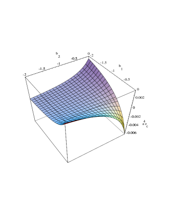
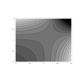
Figure 4: Left: Total integrated Casimir energy per unit-volume times $a^{4}$, i.e. $a^{4}\,\varepsilon_{c}$, corresponding to $D=3$, $-2\leq b_{1}\leq 0$, $-2\leq b_{2}\leq 0$ (in this region, there are no imaginary eigenfrequencies and the p.v. prescription for the integrals is unnecessary). Right: contour representation of the same plot.

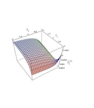
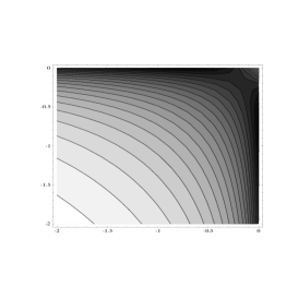
Figure 5: Left: surface contribution $a^{4}\,\varepsilon_{c}^{(2)}$, for $D=3$, $-2\leq b_{1}\leq 0$, $-2\leq b_{2}\leq 0$. For $b_{1}=0$, the minimum at $b_{2}\simeq-0.70$ is visible. Right: associated contour plot.

6 Ending comments

In the present work we have dealt with a calculation of the Casimir energy when one sets Robin boundary conditions on one single plate or a pair of parallel plates. Its evaluation has been based on a variant of the generalized Abel-Plana summation formula in ref.[1], adapted to these situations, and derived in the appendix B. This method turns out to be adequate for finding vacuum expectation values of the energy-momentum tensor, i.e., local densities. From a slightly different viewpoint, zeta function regularization has been applied to the summation of eigenfrequencies, which directly gives the integrated energy per unit-volume.

When just one plate is considered, the only present parameter is the relative coefficient between the non-derivative and derivative terms in the boundary condition ($\beta_{1}$). The local density is given by formula (3.19), which vanishes for the conformal value of the curvature coupling. Otherwise, this formula depicts the local dependence of this density (exemplified by Fig.1 for $D=1$ and $D=3$), which is singular on the plate itself. Note that the requirement of conformal invariance has the power of suppressing the presence of divergent parts, just as happened —for a different system— in ref.[6].

If there are two parallel plates, the relevant parameters are three: the (rescaled) relative coefficients between the non-derivative and derivative parts at each boundary ($b_{1}$ and $b_{2}$), and the separation length between them ($a$). Then, the additional (to a single plate) total integrated Casimir energy per unit-volume is given by formula (5.20), and its decomposition into purely-volume and purely-surface parts by eqs. (4.31) and (5.27), in terms of the quantities $\varepsilon^{(1)}$ and $\varepsilon^{(2)}$ defined by eqs. (4.16) and (4.32). If the coupling is conformal ($\xi=\xi_{c}$), $\varepsilon^{(1)}$ and $\varepsilon^{(2)}$ themselves coincide with the volume and surface contributions, respectively, and, in any case, the decomposition (5.21) holds. The surface contribution, coming from the plates themselves, would be absent for Dirichlet or Neumann boundary conditions.

To be remarked is the fact that, at least in some situations free of imaginary eigenfrequencies, there are parameter choices which give a vanishing Casimir energy. As illustrated by Fig. 3, one may vary the value of the $b_{2}$ parameter so as to reverse the sign of the effect. At the same time, we have seen that there is another $b_{2}$-value for which the surface contribution has a minimum. Examples of simultaneous variations of $b_{1}$ and $b_{2}$ are shown in Figs. 4 and 5.

An interesting feature of the Casimir effect with Robin boundary conditions is that there is a region in the space of parameters defining the boundary conditions in which the vacuum forces are repulsive for small distances and attractive for large distances. This leads to the possibility for the stabilization of the plates separation by using the Casimir effect.

Appendix A Appendix: Complex zeros

First of all we will show that the real and possible purely imaginary zeros (see below) of $F(z)$ are simple. To see this, we note that on the class of solutions to (4.4), the corresponding derivative can be presented in the form

$$F^{\prime}(z)=\left[1+\frac{1}{z}\sin z\cos(z+2\alpha_{1})\right]\left[\left(1-b_{1}b_{2}z^{2}\right)\cos z+(b_{2}+b_{1})z\sin z\right].$$ (A.1)

Using the integral relation

$$1+\frac{1}{z}\sin z\cos(z+2\alpha_{1})=2\int_{0}^{1}dx\,\cos^{2}(zx+\alpha_{1})$$ (A.2)

we conclude from here that $F^{\prime}(z)\neq 0$ if $z$, $z\neq 0$ is a zero of $F(z)$, and hence these zeros are simple.

Purely imaginary zeros of $F(z)$ may exist. This sort of solution has to do with the presence of imaginary parts in the eigenfrequencies. They can be detected as the real zeros of the denominator in the last integral of eq.(B.4). It is convenient to write the corresponding equation in the form

$$\tanh t=\frac{(b_{1}+b_{2})t}{1+b_{1}b_{2}t^{2}}.$$ (A.3)

After studying the nature of this equation in terms of $b_{1}$ and $b_{2}$, one finds out that:

1) Equation (A.3) has no positive real zeros for

$$\left\{b_{1}+b_{2}\geq 1,\ b_{1}b_{2}\leq 0\right\}\cup\left\{b_{1,2}\leq 0\right\}.$$ (A.4)

2) Equation (A.3) has a single positive real zero for

$$\left\{0<b_{1}+b_{2}<1,b_{1}b_{2}\leq 0\right\}\cup\left\{b_{1}+b_{2}\geq 1,b_{1,2}>0\right\}\cup\left\{b_{1}+b_{2}<0,b_{1}b_{2}<0\right\}.$$ (A.5)

3) Equation (A.3) has two positive real zeros for

$$b_{1}+b_{2}<1,\ b_{1,2}>0.$$

The parameter values in Fig. 3, namely $b_{1}=0$ and $-5\leq b_{2}\leq 0$, fall into case 1), when there are no real positive zeros. When $F(z)$ has complex zeros (situations 2 or 3), their extra contribution to the mode sum is given by formula (B.8) in appendix B.

Appendix B Appendix: Summation formula

The vacuum expectation values for the physical quantities in the region between plates will contain the sums over zeros of the function $F(z)$ defined by (4.4). To obtain the summation formula over these zeros we will use the generalized Abel-Plana formula (GAPF) [1]. In this formula as a function $g(z)$ let us choose

$$g(z)=-i\left[\left(1-b_{1}b_{2}z^{2}\right)\cos z+(b_{2}+b_{1})z\sin z\right]\frac{f(z)}{F(z)}.$$ (B.1)

For the sum and difference in the GAPF one has

$$g(z)\pm f(z)=i(b_{1}z\pm i)(b_{2}z\pm i)e^{\pm iz}\frac{f(z)}{F(z)}.$$ (B.2)

Let us denote by $\lambda_{n}$, $n=1,2,\ldots$ the zeros of the function $F(z)$ in the right half-plane, arranged in ascending order, and by $\pm iy_{l}$, $y_{l}>0$ the possible purely imaginary zeros of this function. It can be easily seen that

$${\rm Res}_{z=\lambda_{n}}\,g(z)=\frac{-if(z)}{1+\frac{1}{z}\sin z\cos(z+2\alpha_{1})}$$ (B.3)

(as it follows from (A.2) the denominator on the right of this formula is always positive). First, we will consider the case of function $f(z)$ analytic for ${\rm Re}z\geq 0$. Now substituting in GAPF (formulas (2.10)-(2.11) in [1]) (B.1), (B.2), taking the limit $a\rightarrow 0$ (here $a$ is the parameter on the right of GAPF and the poles $\pm iy_{l}$ are excluded by small semicircles with radius $\rho$ on the right half plane, $\rho\rightarrow 0$), and using (B.3) one obtains the following summation formula

$${\sum_{z=\lambda_{n},\pm iy_{l}}}^{\prime}\frac{\pi f(z)}{1+\frac{1}{z}\sin z\cos(z+2\alpha_{1})} = -\frac{\pi}{2}\frac{f(0)}{1-b_{2}-b_{1}}+\int_{0}^{\infty}f(z)dz+$$ (B.4)

$$+ i\,{\rm p.v.}\int_{0}^{\infty}\frac{\left[f(it)-f(-it)\right]dt}{\frac{(b_{1}t-1)(b_{2}t-1)}{(b_{1}t+1)(b_{2}t+1)}e^{2t}-1}dt,$$

where the prime on the summation sign means that the contribution of terms corresponding to the purely imaginary zeros have to be halved. This contribution comes from the integrals taken around semicircles enclosing these zeros. Note that the denominator on the left can be also written in the form

$$1+\frac{1}{z}\sin z\cos(z+2\alpha_{1})=1-\frac{(b_{1}+b_{2})(1+b_{1}b_{2}z^{2})}{(1+b_{1}^{2}z^{2})(1+b_{2}^{2}z^{2})},\quad z=\lambda_{n},\pm iy_{l}.$$ (B.5)

In (B.4) we have assumed that $b_{1}+b_{2}\neq 1$. In the case $b_{1}+b_{2}=1$ to ensure the convergence at origin in the second integral on the right of formula (B.4) we need to have $f(z)\sim f_{0}z^{\alpha}$, $\alpha\geq 2$, $z\rightarrow 0$. Now the first summand on the right of this formula should be replaced by

$$-\frac{\pi f_{0}\delta_{\alpha 2}}{2(b_{1}^{2}-b_{1}+1/3)}.$$ (B.6)

Formula (B.4) is valid for functions $f(z)$ satisfyng the condition

$$\left|f(z)\right|<\epsilon(x)e^{c\left|y\right|},\quad z=x+iy,\quad\left|z\right|\rightarrow\infty,$$ (B.7)

where $c<2$, $\epsilon(x)\rightarrow\infty$ for $x\rightarrow\infty$, and having no poles on the imaginary axis. However, as follows from (4.10), (4.11), for a scalar field with $\zeta\neq\zeta_{c}$ the corresponding function has the form $f(z)=f_{m}(z)/(z^{2}b_{m}^{2}+1)$, $m=1,2$. In this case the subintegrand on the right of GAPF has purely imaginary poles $\pm i/b_{m}$ for $b_{m}>0$, $m=1,2$. In analogy to the purely imaginary zeros of $F(z)$, these poles have to be excluded from the integral over the imaginary axis by semicircles on the right-half plane. The integrals over these semicircles will give additional contributions

$$-\frac{\pi}{2\left|b_{m}\right|}\theta(b_{m})\left[f_{m}(e^{\pi i/2}/\left|b_{m}\right|)+f_{m}(e^{-\pi i/2}/\left|b_{m}\right|)\right].$$ (B.8)

to the right-hand side of (B.4). In the case $b_{1}=-b_{2}$ and for functions $f(z)$ having no poles on the imaginary axis from (B.4) one obtains the Abel-Plana formula in the usual form.

References

• [1] A. A. Saharian, Izv. AN Arm. SSR. Matematika 22 (1987) 166 (Sov. J. Contemp. Math. Analysis 22 (1987) 70); A. A. Saharian, The generalized Abel-Plana formula. Applications to Bessel functions and Casimir effect. Preprint IC/2000/14, hep-th/0002239.
• [2] G. Plunien, B. Müller and W. Greiner, Phys. Rep. 134 (1986) 87; V. M. Mostepanenko and N. N. Trunov, The Casimir Effect and its Applications, Oxford Univ. Press, 1997; K.A. Milton, The Casimir Effect: Physical Manifestations of the Zero-Point Energy, hep-th/9901011.
• [3] T. H. Boyer, Phys. Rev. 174 (1968) 1764; B. Davies, J. Math. Phys. 13 (1972), 1324; R. Balian and B. Duplantier, Ann. Phys. (N.Y.) 112 (1978) 165; K. A. Milton, L.L. De Raad Jr. and J. Schwinger, Ann. Phys. (N.Y.) 115 (1978) 388.
• [4] S. Leseduarte and A. Romeo, Ann. Phys. (N.Y.) 250 (1996) 448.
• [5] V. V. Nesterenko and I. G. Pirozhenko, Phys. Rev. D57 (1997) 1284; M. E. Bowers and C. R. Hagen, Phys. Rev. D59 (1999) 025007.
• [6] E. Elizalde and A. Romeo, Int. J. Mod. Phys. A 5 (1990) 1853.
• [7] G. Kennedy, R. Critchley and J. S. Dowker, Ann. Phys. 125 (1980) 346.
• [8] D. Deutsch and P. Candelas, Phys. Rev. D 20 (1979) 3063; P. Candelas, Ann. Phys. 143 (1982) 241.
• [9] N. D. Birrel and P. C. W. Davis, Quantum fields in curved space, Cambridge University Press, 1982.
• [10] M. R. Setare and A. A. Saharian, Int. J. Mod. Phys. A16 (2001) 1463.
• [11] S. N. Solodukhin, Phys. Rev. D63 (2001) 044002.
• [12] V. M. Mostepanenko and N. N. Trunov, Sov. J. Nucl. Phys., 42 (1985) 812.
• [13] I. G. Moss, Class. Quantum Grav. 6 (1989) 759.
• [14] G. Esposito and A. Yu. Kamenshchik, Class. Quantum Grav. 12 (1995) 2715.
• [15] T. Ghergetta and A. Pomarol, Nucl. Phys. B586 (2000) 141.
• [16] C. M. Bender and K. A. Milton, Phys. Rev. D50 (1994) 6547; K. A. Milton, Phys. Rev. D55 (1997) 4940.
• [17] A. A. Saharian, Phys. Rev. D63 (2001) 125007.
• [18] A. Romeo and A. A. Saharian, Phys. Rev. D63 (2001) 105019.
• [19] A. P. Prudnikov, Yu. A. Brychkov and O. I. Marichev, Integrals and series, v.1, 1986.
• [20] M. Abramowitz and I. A. Stegun, Handbook of Mathematical functions, National Bureau of Standards, Washington D.C., 1964.
• [21] J. Ambjørn and S. Wolfram, Ann. Phys. 147 (1983) 1.
• [22] L. S. Brown and G. J. MacLay, Phys. Rev. 184 (1969) 1272; D. B. Ray and I. M. Singer, Adv. Math. 7 (1971) 145; A. Salam and J. Strathdee, Nucl. Phys. B90 (1975) 203; J. S. Dowker and R. Critchley, Phys. Rev. D13 (1976) 3224; S. W. Hawking, Commun. Math. Phys. 55 (1978) 133; R. Kantowski and K. A. Milton, Phys. Rev. D36 (1987) 3712.
• [23] S. K. Blau, M. Visser, and A. Wipf, Nucl. Phys. B310 (1988) 163.