Concepts in Gauge Theory Leading to Electric–Magnetic
Duality
TSOU Sheung Tsun
Mathematical Institute, Oxford University
24–29 St. Giles’, Oxford OX1 3LB
United Kingdom.
tsou @ maths.ox.ac.uk
Abstract
Gauge theory, which is the basis of all particle physics, is itself based on a few fundamental concepts, the consequences of which are often as beautiful as they are deep. In this short lecture course I shall try to give an introduction to these concepts, both from the physical and mathematical points of view. Then I shall show how these considerations lead to a nonabelian generalization of the well-known electric–magnetic duality in electromagnetism. I shall end by sketching some of the many consequences in quantum field theory that this duality engenders in particle physics.
These are notes from a lecture course given in the Summer School on Geometric Methods in Quantum Field Theory, Villa de Leyva, Colombia, July 1999, as well as a series of graduate lectures given in Oxford in Trinity Term of 1999 and 2000.
Synopsis
-
•
Gauge invariance, potentials, fields
-
•
Yang–Mills theory in action—the Standard Model of particle physics
-
•
Principal bundles, connections, curvatures
-
•
Gauge group and charges
-
•
Action principle and symmetry breaking
-
•
Electric–magnetic duality
Introduction
In this lecture course I shall be mostly concerned about some basic concepts of gauge theory, mainly to answer the question: why are they introduced in physics? Almost all of these concepts appear already at the classical level, so that we shall deal principally with the motion of a quantum charged particle in a classical (gauge) field. In so doing we shall find that certain fundamental questions will arise which are usually not addressed by physicists, because they are usually overwhelmed by many seemingly more pressing questions.
As a by-product, I shall also try to clarify a few notations to make it easier for mathematicians to read physics literature.
Since Maxwell’s theory of electromagnetism, that is, abelian gauge theory, is the best understood gauge theory, I shall take it as our reference point. So most definitions will start with the abelian case, and most results will be checked against it. However, we shall be extremely careful in not assuming abelian results for the nonabelian case.
For most of the basic concepts, I shall be following my book. Apart from other textbooks both in mathematics and physics which I have found useful, I have included in the bibliography only a few papers. For those who are interested to pursue further, the references in the cited material will easily lead them to other relevant articles.
1 Gauge invariance, potentials, fields
In the first lecture, I shall use very simple mathematics only, so as to put the emphasis on the physical reasons behind these concepts. In subsequent lectures, however, I shall not hesitate to use more sophisticated mathematics, because it helps both in further understanding and further developments. In this way, I hope to show you that it is the physical situations which force us to use various sophisticated mathematical tools, and not the other way round, by which I mean looking for or inventing physical theories to apply the mathematical tools we have on hand.
1.1 Notations and conventions
I shall use the following groups of terms synonymously:
-
•
Maxwell theory, theory of electromagnetism, abelian theory;
-
•
Yang–Mills theory, nonabelian (gauge) theory (however, nonabelian may take a truly mathematical meaning);
-
•
Spacetime, Minkowski space.
I shall use the following notations unless otherwise stated:
-
•
= Minkowski space with signature
-
•
= spacetime indices = 0,1,2,3
-
•
= spatial indices or group indices
-
•
repeated indices are summed
-
•
= gauge group = compact, connected Lie group
(usually )
I shall make the following convenient assumptions: functions, manifolds, etc. are as well behaved as necessary; typically functions are continuous or smooth, manifolds are .
I shall use the units conventional in particles physics, in which , the former being the reduced Planck’s constant and the latter the speed of light.
Caveat In a fully quantized field theory, particles and fields are synonymous. Where there is no confusion, I shall use the two terms interchangeably.
1.2 Gauge invariance, potentials, fields: abelian case
Consider an electrically charged particle in an electromagnetic field. The wavefunction of this particle is a complex-valued function of (spacetime). The phase of is not a measurable quantity, since only can be measured and has the meaning of the probability of finding the particle at . Hence one is allowed to redefine the phase of by an arbitrary (continuous) rotation independently at every spacetime point without altering the physics. We say then that this theory possesses gauge invariance or gauge symmetry.
In view of this arbitrariness, how can we compare the phases at neighbouring points in spacetime? In other words, how can we ‘parallelly propagate’ the phase? We can, if we are given a vector-valued function , called the gauge potential. Then for the phases at and a nearby point to be ‘parallel’ we stipulate that the phase difference be , where is a proportionality constant which will later be identified with the charge of the particle. This concept of ‘parallellism’ has to be consistent with gauge invariance. In other words, if we effect a rotation of on the phase of ,
then the phase rotation at will be
so that for consistency the gauge potential must transform as
Next, by iterating the parallel phase transport along a given path , we can obtain a finite phase difference:
This depends on the path in general.

Now the phase difference (with )
at the same point (see Figure 1) is a physically measurable quantity (as observed in interference phenomena), depends on the potential, and is in general nonzero. By Stokes’ theorem
where The quantity is the infinitesimal phase change on going round the infinitesimal parallelogram , Figure 2:
It follows that the tensor is a gauge invariant quantity, as can be checked directly. Now this change in phase, apart from the factor representing the charge of the particle in question, acts on all wavefunctions in a universal way and is hence a physical property of the spacetime under consideration. It represents therefore a physical field, called the electromagnetic field tensor.
Historically, in classical physics, it was the components of this field tensor, the electric and magnetic fields, which were introduced first:
The potential was introduced as a mathematical convenience only, since in classical physics it is not necessary to specify the potential, only the field.
Bohm–Aharonov experiment
To demonstrate that in order to describe fully quantum mechanics in electromagnetism one needs the potential, not just the field, Bohm and Aharonov devised the following experiment, successfully performed by Chambers.
Electrons are made to travel along two different paths and , as illustrated in Figure 3, enclosing a magnetic core. Outside this magnetic core, the field vanishes but the potential is nonzero. A diffraction pattern, made by the interference of the two beams, is observed on the screen beyond the magnetic core, and this diffraction pattern varies as the magnetic field and the paths are varied, according to the phase difference we calculated above.
This is one of the most important experiments of modern physics, and its positive outcome is widely regarded as the strongest single evidence supporting the basic tenets of electromagnetism as a gauge theory.
1.3 Gauge invariance, potentials, fields: nonabelian case
Yang–Mills theory, as originally proposed by Yang and Mills in 1954, is a generalization of electromagnetism in which the complex wavefunction of a charged particle is replaced by a wavefunction with 2 components . By a change of ‘phase’ we now mean a change in the orientation in internal space of under the transformation:
where, to preserve probabilities, is to be a unitary matrix. In this way, gauge invariance can now be interpreted as the requirement that physics be unchanged under arbitrary transformations on independently (but continuously) at different spactime points. We note that it is also possible to have the more general transformations.
We can now consider parallel transport of this ‘nonabelian phase’ in a way similar to the abelian case. Introducing the gauge potential as a matrix-valued spactime vector-valued function, we again stipulate that at two neighbouring points and , the ‘phases’ are parallel if they differ by , where the porportionality contant again represents a ‘charge’:
Note that now , because it represents an infinitesimal change in the phase of . Under a gauge transformation , so that
But
where is the gauge transform of .
Equating, we get, for all ,
Expanding to leading order in and dropping ,
When is infinitesimal, in the sense
then we get
which reduces to our previous formula in the abelian case.
Next, we consider transport over a finite path as before. Remembering that our primary concern is how the wavefunction changes, we see that what matters is the limit of the product of the matrices as the step size tends to zero, and not the sum of the ‘phases’ . (Remember we are being unsophisticated!) For matrices, in general , so that the answer we are after is not
but the product of as we said. However, for sentimental reasons about the abelian case, this product is usually written
where the letter denotes path-ordering. This Yang called the Dirac phase factor; it is also known as the Wilson loop.
For a closed infinitesimal path in the form of a rectangle , Figure 2, we can evaluate the change in phase as before (where repeated indices on the right are not summed):
Hence the phase difference at , on expanding to leading order,
As before, we can define the field tensor by equating this to
whence
By similar considerations as before, we see that under a gauge transformation , transforms as
We see that is no longer gauge invariant, as in the abelian case, but gauge covariant.
Important Remarks
-
1.
In the above description of classical electromagnetism the gauge group symmetry (that is, the phase freedom) plays no role (or only a trivial one) if there are no charges, because , the physical fields, are gauge invariant. However, when we consider the dynamics in the form of the Maxwell equations, then this symmetry is the symmetry of those equations, and is therefore an important ingredient even in the classical field theory without charges. This remark does not apply to Yang–Mills theory, since there the field being covariant and not invariant the gauge symmetry should be taken into account already at the outset.
-
2.
We note an extremely important difference betwen the abelian and the nonabelian case: the finite phase difference is no longer related to the surface integral of the field tensor in the nonabelian case. First, the Dirac phase factor is not given by a line integral along the closed path . In fact, the line integral has no significance at all in the nonabelian case. Moreover, the surface integral of does not make sense, since there is no way to order the matrices on a surface!
-
3.
Because it is only covariant and not invariant the field tensor here is no longer a physically measurable quantity, not even in classical physics.
-
4.
Yang has shown that, both in abelian and nonabelian theories, what describes the physics exactly is the Dirac phase factor in the sense that the same physical situations correspond to identical and different physical situations to different . The obvious question then arises: why do we not use as variables to describe Yang–Mills theory and forget about the gauge dependent potential ? The answer is: the space of of closed loops is infinite dimensional, which means that is more difficult to handle, and there are vastly too many variables. Roughly speaking, we would be using functions of infinitely many variables as opposed to 4 functions of 4 variables! We shall have a bit more to say on this later.
2 Yang–Mills theory in action—the Standard Model of particle physics
Before we proceed any further and in order to exhibit the pivotal role that Yang–Mills theory plays in modern physics, I have to tell you some facts about particles. This lecture is strictly for mathematicians only!
2.1 Particle classification
Particles are classified by their interactions among themselves and with the fields in spacetime. Apart from gravity, which we shall neglect totally in these lectures, there are two kinds of interactions: strong and electroweak. Both are gauge theories, but with a significant difference. We shall take them in turn presently.
Fundamental particles are also distinguished by their spin. Particles with integral spins (in suitable units) are called bosons, and those with half-(odd)-integral spins are called fermions. Known bosons all have spin 1, and are sometimes called vector bosons. There are some spin 0 bosons, called scalars, which are postulated to exist but have not yet actually been detected. All known fermions have spin . Fermions which take part only in electroweak interactions are called leptons.
There are many (all unstable) particles called resonances which are composites of those above. (The only possibly stable composite is the proton.) They are mainly divided into mesons (such as pions) or baryons (such as protons, neutrons), but we shall not study them here. There are more than 150 such so far discovered.
For our purposes, the following are the fundamental particles:
Vector bosons (also known as gauge bosons): ; ;
(photon; massive vector bosons; gluons)
Leptons: ; ;
(electron, electron neutrino; muon, muon neutrino; tauon, tau neutrino)
Quarks: ; ;
(up, down; charm, strange; top, bottom)
In a full quantum theory, these particles all have corresponding antiparticles. The notation is: the antiparticle of is denoted .
Remarks
Fact 1. All known fundamental bosons have spin 1.
Fact 2. All known fundamental fermions have spin .
Fancy 1. ( Fact 3.)
Theory postulates existence of certain scalars called Higgs particles.
Fancy 2. Supersymmetry needs spins .
Terminology changes as our understanding goes further.
2.2 The strong interaction
The strong interaction gives rise to nuclear forces and is governed by an gauge theory. This gauge symmetry is fancifully called “colour”, and so the corresponding quantum field theory is usually called quantum chromodynamics or QCD.
The gauge potential takes value in the Lie algebra , and has hence 8 components. Interpreting these as particles (when the field is fully quantized), they form the 8-dimensional adjoint representation of . They are called the gluons. They are vector bosons and are massless. They do not have electric charges.
The massive particles are in the 3-dimensional fundamental representation of . These are called quarks. They are spin fermions, and have charges of or , in units of the electron charge. There are 6 known species of quarks: ; each of which has 3 components corresponding to . These components are said to have different “colours”, e.g. red, green and blue. These have no relation to the genuine colour that we see.
Just as the phase in electromagnetism can be arbitrarily rotated at each spacetime point, and so cannot be measured, so is this colour symmetry. We say in both cases that the gauge symmetry is exact. Where QCD differs from QED is that particles with nontrivial colour charges, i.e. in any representation of other than the trivial one, cannot exist in the free state. They cannot therefore be directly observed, but indirectly their existence is fairly well established experimentally. This peculiar property goes under the name of confinement and is special to nonabelian theories. To prove confinement is one of the most important aims of theoretical physics at present. Experimentally this is true so far, since only singlets of have ever been observed. This is the probable origin of the name “colour”, as in the hidden colours of white light.
Quarks and antiquarks combine to produce observable particles as resonances. We can see which combinations are possible by looking at the tensor product of the fundamental and conjugate fundamental representations and picking out the singlet. For example:
Thus we have:
Ordinary mesons are states, and ordinary baryons are states. In principle one can have higher composites and some such exotics as may have been already observed.
2.3 The electroweak interaction
The electroweak interaction gives rise to both electromagnetic phenomena and radioactivity, and is governed by a gauge theory with a gauge group usually denoted as . (We shall give more details about the specification of the exact gauge group in Lecture 4.) The part is often referred to as (weak) isospin, and the part as (weak) hypercharge.
In electroweak (or Weinberg–Salam) theory an important novel ingredient is introduced in Yang–Mills theory, that is, (spontaneous) symmetry breaking. In addition to the gauge bosons (vector bosons) and the massive fermions as in QCD, we introduce some scalar (i.e. spin 0) particles called Higgs fields . They are in a 2-dimensional representation so that they are in fact gauge spinors:
The lowest energy state (called vacuum) occurs when , so that a physical system in such a vacuum state corresponding to will no longer be invariant under the whole of , only under a subgroup which leaves the spinor invariant. This is the situation of symmetry breaking: although the theory has invariance, the actual physical system has a smaller invariance. This subgroup is generated by a linear combination of and , where are the generators of and is the generator of weak hypercharge . (We shall go into more details later.)
Reminder. The notation for is exactly the same as for ordinary spin, where is represented by the diagonal matrix
and the commutation relation is .
The residual gauge group is identified with the gauge group of electromagnetism, as observed in the physical world.
The mechanism of symmetry breaking is often visualized as a phase change. In the early universe when the temperature was high, the whole symmetry was exact. As the temperature decreased to a critical value, symmetry breaking occurred and the electromagnetic gauge symmetry “froze out” to produce the phase we are in today.
As a result of the symmetry breaking, 3 of the 4 gauge bosons combine with some components of the Higgs doublet to become massive vector bosons (). The boson corresponding to remains massless and is the photon of the electromagnetic field.
The leptons are the fermions of the theory. The charged leptons are , and the neutral leptons are the neutrinos . Each lepton wavefunction can be projected into 2 mutually orthogonal components:
Since has spin , it is a spacetime spinor and and are eigenstates of the chirality operator . Then the representation assignments are:
Notice that neutrinos are supposed to have only left-handed components in this assignment. In view of the recent SuperKamiokande results on neutrino oscillations, it may be necessary to revise this assignment and suppose the neutrinos have also right-handed components (and a nonzero mass).
2.4 The Standard Model
The particle spectrum is summarized in Table 1. Note that the particles in brackets are not (or have not been) directly observed, but they are part of the gauge theory.
The standard model is an amalgamation, a knitting together, of the above two theories in such a way that all of known particle physics, up to the present day, is encompassed. It is a Yang–Mills theory with a gauge group which is usually written as —we shall examine this in more detail in Lecture 4. The particle content can be schematically represented as
(QCD + Weinberg–Salam) 3.
The multiplication by 3 is necessary to model another aspect of the particle spectrum known as generation. Take the charged leptons as an example. There are 3 of them: . Except for their very different masses:
they behave in extemely similar fashions. The 3 neutrinos also have similar interactions. The quarks also come in 3 generations: with charge (called the up-type quarks) and with charge (called the down-type quarks).
But the standard model is not just putting the 2 theories together, because although the leptons do not transform under (since they have no strong interaction), the quarks are in nontrivial representations of weak isospin . In fact, we can set up Table 2 for the 3 generation, and Table 3 for the lightest generation (and similar ones for the other two generations).
In Table 3 the electric charge satisfies: . Other normalizations exist in the literature.
The standard model is a very good representation of the state of our present knowledge, but most physicists doubt that it constitutes a full final theory.
Good points
-
1.
Purports to explain all of particle physics.
-
2.
Survives all precision tests so far.
Open questions
-
1.
Why 3 copies (generations)?
-
2.
Where do the Higgs fields come from?
-
3.
Why are quarks confined?
-
4.
There are over 20 parameters which are not explained by the theory.
3 Principal bundles, connections, curvatures
In this lecture we change tack altogether and make contact with differential geometry. Most mathematicians working on Yang–Mills theory work on vector bundles, but following Yang I tend to think in terms of principal bundles. The two ways are of course equivalent.
In order to simplify definitions and so on and avoid all unnecessary troubles, I shall make the following general assumption:
‘Things are as nice as possible.’
For example, manifolds and maps are smooth, Lie groups are compact connected, equivalence classes can be confused with their representatives.
Also, no formal proofs will be given.
3.1 Principal bundles
Definition. A principal coordinate bundle is a collection of the following:
-
1.
a manifold called the total space,
-
2.
a manifold called the base space,
-
3.
a projection , with , called the fibre above ,
-
4.
a Lie group acting on itself by left translation, called the structure group,
-
5.
an open cover of ,
-
6.
, a diffeomorphism called coordinate function
satisfying
-
(a)
,
-
(b)
if we define
then on the overlap the composite
is the left multiplication by a uniquely determined element of ,
-
(c)
the map
is smooth—it is called the transition or patching function.
-
(a)
A sketch (Figure 4) may be helpful.

Definition. Two principal coordinate bundles and are said to be strictly equivalent if they have the same total space , the same base space , the same projection , the same structure group , and their coordinate functions are such that the composite
is left multiplication by an element of .
Definition. A principal bundle is an equivalence class of coordinate principal bundles under strict equivalence.
Definition. A trivial principal bundle is one in which
This is the case in most applications to physics.
Note. We shall often call the principal bundle.
Dictionary 1
| base space | spacetime | |
| structure group | gauge group | |
| principal bundle | gauge theory | |
| principal coordinate bundle | gauge theory in a particular gauge |
3.2 Connections and curvatures
First we recall a few definitions.
-
1.
Give a map we can define its differential at , as a linear map as follows. Given a tangent vector at , choose any curve in such that and is the tangent to at . Then the image is the tangent vector to the image curve in at . It can be shown that the definition is independent of the curve . Similarly, given any 1-form on , we can define a 1-form on by
for any vector field on .
-
2.
Denote by the left multiplication by an element . Let be the Lie algebra of . A vector field on is said to be left invariant if . Recall then that can be characterized as the set of left invariant vector fields on .
-
3.
Suppose a group acts on the right on a manifold . Then for each , the action induces a vector field on as follows. At each , consider the action of the 1-parameter subgroup , whose orbit is a curve in passing through at . The tangent to the curve at is the required vector. We call the fundamental vector field corresponding to .
Now we come to the definition of a connection on . Consider the action of on given by, ,
where . Note that this action moves points along the same fibre, and is indeed a right action since . We also write: .
Definition. Given a principal bundle as above, a connection 1-form on is a -valued 1-form on satisfying
-
1.
,
-
2.
vector fields on , where the adjoint action ad of on is often written as .
We wish now to show how to define, using a set of local sections , local 1-forms which are equivalent to the given connection .
Choose local sections such that
Then Let be a tangent vector of at ; then
We have
Now define . So acting with on both sides we get
Now and is the vector corresponding to the fundamental vector field at . Hence we have
This is to be compared with our formula from Lecture 1:
In fact, since goes from patch to patch , and goes from unprimed to primed patch, we should re-write this last formula by using :
which, apart from the physical dimensional factor , is exactly the same as the first formula.
[Reference. Tanjiro Okubo: Differential Geometry, Marcel Dekker Inc., New York and Basel, 1987.]
In particular, we see that which is a 1-form on can be replaced by a collection of 1-forms on . In the special case when the principal bundle is trivial, we need only one such 1-form on . This is the usual case in physics.
A connection on defines a decomposition of the tangent space at each point into a vertical and a horizontal subspace:
where consists of all those tangent vectors which are tangent to the fibre through , and those tangent vectors annihilated by .
Definition. We can now define the exterior covariant derivative of a -form by
where denotes the horizontal component of .
Definition. The curvature 2-form of the connection is defined by .
Theorem. (The structure equation of Cartan)
Theorem. (Bianchi identity)
Definition. We say that a connection is flat if .
Definition. One can also define local curvature forms:
It can then be shown that the following patching condition holds:
Dictionary 2
| connection | gauge potential | |
| curvature | gauge field |
Translation. (The structure equation of Cartan)
(This formula appeared in Lecture 1.)
Translation. (Bianchi identity)
where
3.3 Bundle reductions
Let be a principal bundle with structure group and let be a subgroup. We say that is reducible to if there exists an open cover of such that all the transition functions take value in . Then a reduced subbundle or reduction has as total space such that such that .
Given a reduction we have the associated bundle with fibre , structure group , and total space . Then we have
Proposition. There exists a 1–1 correspondence between sections and reductions . [See Steenrod’s book, in the Bibliography.]
When we consider a connection on , it may happen that when restricted to takes value in the Lie algebra of . Equivalently, for all is tangent to . In this case, we say that the connection is reducible to .
Dictionary 3
| bundle reduction | symmetry breaking | |
|---|---|---|
| section | Higgs fields |
Examples. To be given later.
3.4 Holonomy and loop space variables
Consider a principal bundle . Let , be a piecewise differentiable curve in . Then a horizontal lift of , denoted by , is a curve in such that , and all its tangent vectors are horizontal. Through any point such that there is a unique horizontal lift of which starts at .
Suppose now we are given a curve in starting from and ending in . Let be an arbitrary point in , and consider the horizontal lift of through . Let be its end-point, so that we have . Thus the horizontal lift defines a map which we call the parallel transport of the fibre above to the fibre above . It can be proved that (i) this map is an isomorphism and that (ii) it is independent of the parametrization of the curve . [Reference: Kobayashi and Nomizu, p.70.]
Suppose next that the curve in is closed, that is . Then the parallel transport is an isomorphism of to itself. By considering all piecewise differentiable closed curve through , it is easy to see that the parallel transports form a group of automorphisms of , called the holonomy group through , which can be identified with a subgroup of the structure group . It can be shown that if is connected, then all holonomy groups through any given are conjugate to one another and are hence isomorphic. Therefore, if we are concerned only with the abstract holonomy group for a given connection and not which particular subgroup of it is, then we can omit the reference to . We can thus consider simply the holonomy of a closed curve in as an element of .
Dictionary 4
holonomy phase factor
(Compare Lecture 1.)
Note. The curvature at a given point can again be thought of as the holonomy of an infinitesimal closed looop through that point.
Flat connections
Suppose is connected. If is not simply connected, then a flat connection may give rise to nontrivial holonomy. In fact, there is a 1–1 correspondence:
Let be the space of closed piecewise differentiable loops in , called the loop space of . For convenience, we always consider loops starting and ending at a fixed point . Given any connection , the holonomy defines a map
which satisfies the composition law. This means that given two loops and , we can compose them to give a third loop , by first going round for and then going round for , for instance. Then we have
where the product on the right-hand side is group multiplication.
The converse problem: given a map satisfying the composition law (and some other obvious conditions), can one define a connection of which is its holonomy? This problem has great importance for Yang–Mills theory and is to a large extent solved. However, the known proofs are all hard and not totally rigorous. We shall not present them here.
It is, however, interesting to see why the problem is of importance to Yang–Mills theory.
I mentioned in Lecture 1 that Yang proved that the Dirac phase factor describes gauge theory exactly, in the sense that there is a 1–1 correspondence between
This is in contrast to the variables which depend on gauge (which means coordinate bundle in the language of this Lecture), or the variables , which cannot distinguish all physically different situations. However, we have to be extremely careful in not confusing this with the concept of redundancy. A moment’s thought will tell us that not all maps
come from a connection, and further study will reveal the fact that adding the composition law (and certain other obvious conditions) is not enough. In other words, we have to impose constraints on the variables .
The situation can be summarized as follows. If we use the variables , then the physically relevant objects are equivalence classes of under gauge equivalence. If we use the variables , then we have to find the relevant subset by imposing constraints. Depending on the problem at hand, it is sometimes easier to deal with the quotient space (the case of ) or to deal with a subspace (the case of ).
I shall now give a rough non-rigorous description of what the main constraint is. Given a closed loop , we can make a -function variation at any point on the curve. As the height of this -function goes to zero, we can then define the loop derivative of any loop-dependent quantity. Remembering that is an element of , we define the Lie algebra-valued quantity as the logarithmic derivative of :
This can be illustrated by the sketch in Figure 5. In asmuch as this quantity carries the phase factor from one loop to
a neighbouring loop, it is like an infinitesimal phase transport and can indeed be regarded as some sort of “connection” in a coordinate bundle over . We can even go further and consider its holonomy, this time of a closed loop in , which means a closed surface in .
The constraint we are after is that this connection be flat. We note that this does not necessarily imply that the corresponding holonomy is trivial. Any such nontrivial holonomy can be interpreted as a nonabelian magnetic monopole charge, as we shall see.
4 Gauge group and charges
4.1 Locally isomorphic semi-simple Lie groups
So far, we have been rather vague about the exact gauge group that occurs in a particular Yang–Mills theory. A particularly interesting, but often neglected, aspect is the different choices of Lie groups which correspond to the same Lie algebra. In asmuch as the Lie algebra can be identified (as a vector space) with the tangent space at the identity, it is clear that groups which are locally isomorphic (that is, quotients by discrete subgroups) have the same Lie algebra. In fact, for semi-simple groups, among all locally isomorphic groups there is one which is simply connected and which is the universal cover of all the others. These latter can then be obtained from the universal cover group by factoring out by various subgroups of its (discrete) centre.
Some examples will make this clear.
-
1.
Consider the matrix groups and . The Lie algebra of consists of skew matrices, and we can choose as generators:
which satisfy the commutation relations
The Lie algebra of consists of the trace-free skew hermitian matrices, and we can choose as generators:
where are the Pauli matrices
They satisfy
Hence the two Lie algebras are isomorphic. The groups are not isomorphic, only locally isomorphic. In fact, there is a 2–1 map
in such a way that is a double cover of . This map can easily be worked out explicitly (Exercise).
More generally, we can think of as the unit sphere in , by identifying with unit quaternions (). Then the 2–1 map corresponds to identifying antipodal points of .
Furthermore, this discrete quotient is by the centre of , and this discrete group is the fundamental group of .
-
2.
Very similar considerations apply to , with centre . In the case of , we have altogether 2 locally isomorphic groups: and . In the case of we have 4:
where and are subgroups of the centre .
-
3.
The group is a double cover of , the covering map being given by multiplication as follows. First embed by
Then
We see immediately that and have the same image in .
4.2 Specification of the gauge group
Recall (Lecture 1) that gauge invariance comes about as the invariance of the wavefunction of a charged particle under the action of a group , so that to specify one has to examine all the charged particles occurring in the theory, in other words, its spectrum.
Start with electromagnetism. Under a phase rotation, , so that we can parametrize the circle group corresponding to the phase by .
Next suppose there are charges in the theory; then . If the charges are commensurate, that is, if there exist and integers such that
then again we can parametrize the by , because if changes by any integral multiple of , the wavefunctions corresponding to all the charges will be unchanged. If, however, there is at least one pair of charges whose ratio is irrational, then we no longer have as a gauge group. In fact, charge quantization is equivalent to having as the gauge group of electromagnetism.
On the other hand, if we consider pure electromagnetism without charges, then the only relevant gauge transformation are those of :
so that the group will just be the real line given by the scalar function .
Similar considerations apply to nonabelian theory. In the vast majority of cases, from the physics point of view, one knows the Lie algebra, and then one needs to inspect the spectrum to get the correct Lie group. One must bear in mind that this implies, for any given Yang–Mills theory, that if in future the spectrum is changed for any reason, one may have to consider another Lie group instead.
Consider first a pure Yang–Mills theory without charges, so that the only gauge transformation one needs to consider is on the gauge potential :
Let be the universal cover of all the groups corresponding to the given Lie algebra. Then the effects on of and , where is an element of the centre of , are identical. Hence the correct gauge group must be , which is in an obvious sense the smallest of all the possible groups. So in the example (1) we considered, the group is and not .
On the other hand, if the theory contains particles with a 2-component wave function , then
and the effect of and are not identical. Hence in this case the correct gauge group is indeed and not .
These considerations can also be cast in terms of representations. Charged particles in a Yang–Mills theory are in certain representations of the gauge group. What we are saying is the known result that the collection of all representations determines the group. In the above case, the gauge potential is in the 3-dimensional adjoint representation and the 2-component is in the 2-dimensional spinor representation. In the absence of the spinor representation, the group is , but when spinors are present, the group must be . This representation theory is entirely identical to the theory of spin and angular momentum in quantum mechanics.
We now apply these considerations to the Yang–Mills theories occurring in particle physics. For these we suppress the gauge couplings for convenience.
-
1.
Strong interaction. Because we postulate the existence of quarks, which are in the 3-dimensional fundamental representation of , we conclude the gauge group is indeed .
-
2.
Electroweak interaction. The particles are of 2 types (where ‘flavour’ means ‘weak isospin’):
-
(a)
flavour doublets with half-integral weak hypercharge— odd;
-
(b)
flavour singlets or triplets with integral weak hypercharge—.
Under a gauge transformation generated by the generators and , we have for the two types of particles:
so that the resultant action of in both cases is the identity. Hence we conclude that in the group we should identify pairs , so that the correct gauge group for electroweak theory is .
However, if in future we either discover or postulate more particles, e.g.
-
(c)
flavour doublets with integral weak hypercharge, and/or
-
(d)
flavour singlets or triplets with half-integral weak hypercharge,
then the effect of and on these particles are distinct, and in that case the correct group is .
-
(a)
-
3.
Standard model. Similar considerations of the known/postulated spectrum, as given in Lecture 2, will show that we should have a 6-fold identification in , where the following 6 triplets should be identified:
where and are elements respectively of , and , with:
and
with obvious embeddings in and abuse of notation (same symbol for generators of different representations).
4.3 Charges and monopoles
We have known for a long time what the electric charge is. There are several equivalent ways of defining or describing it. For our purpose here, we shall consider it as giving a nonvanishing right hand side to Maxwell’s equation:
where the current is given in one of two ways111In the above I have introduced the gamma matrices , which are important ingredients in Dirac’s theory of the spin particles and which provide a prosaic way of using Clifford algebras. For lack of time I shall not expand into the subject, but they are treated in depth in Hijazi’s lectures. See also the lectures of Langmann.:
The quantity here in fact plays a double role:
-
(a)
it is the electric charge—it determines how the charge interacts with the field, and
-
(b)
it is the coupling constant—it fixes the strength of the interaction.
In Yang–Mills theory, a non-abelian electric charge (sometimes referred to generically as a “colour electric charge”) can also be thought of as giving a non-vanishing right hand side to the Yang–Mills equation:
where for the quantum particle. [In Yang–Mills theory, one does not usually concern oneself with classical charges.]
But here the two roles (a) and (b) are quite distinct. The wavefunction is in a certain representation of the gauge group , and how the particle interacts with the gauge field is determined by the representation, the interaction being given by the covariant derivative. The coupling constant , on the other hand, is the numerical factor which fixes the strength of the interaction.
We see that both abelian and nonabelian electric charges occur as nonvanishing currents. In order to make a practical distinction between these and the topological charges we shall discuss next, let us call them electric charges, or simply charges when there is no confusion.
There is another type of charges called monopoles. They are typified by the magnetic monopole as first discussed by Dirac in 1931.
To understand them better, let us look at Maxwell’s equations both in the 3-vector and 4-vector notations:
Here the charge density and the electric current together form the 4-current . We also define the dual field tensor by
where is the totally skew symbol with the convention that .
At the classical particle level, these equations simply tell us the experimental fact that magnetic charges, called magnetic monopoles, do not exist in nature. If, on the other hand, we are concerned with quantum particles, then the Bohm–Aharonov experiment (Lecture 1) tells us that we have to introduce the vector potential bearing the relation with the field as
Simple algebra will tell us that this implies as above. Hence we conclude that:
The result is actually stronger. Suppose there exists a magnetic monopole at a certain point in spacetime, and without loss of generality we shall consider a static monopole. If we surround this point by a (spatial) 2-sphere , then the magnetic flux out of the sphere is given by
where and are the northern and southern hemispheres intersecting at the equator . By Stokes’ theorem since has no components ,
where means the equator with the opposite orientation. Hence . But this contradicts the assumption that there exists a magnetic monopole at the centre of the sphere. Hence we see that if a monopole exists, then will have at least a string of singularities leading out of it. This is the famous Dirac string.
The more mathematically elegant way to describe this is that the principal bundle corresponding to electromagnetism with a magnetic monopole is nontrivial, so that the gauge potential has to be patched (i.e. related by transition functions). [Recall the collection of local 1-forms .] Consider the example of a static monopole of magnetic charge . For any (spatial) sphere of radius surrounding the monopole, we cover it with two patches :
and define in each patch:
In the overlap (containing the equator), and are related by a gauge transformation
Notice that has a line of singularity along the negative -axis (which is the Dirac string in this case). Similarly for .
Furthermore, the corresponding field strength is:
If we now evaluate the ‘magnetic flux’ out of , we have
in other words, in the presence of a magnetic monopole the last two Maxwell’s equations are modified:
with
How are the charges and related? Well, the gauge transformation relating and must be well-defined, that is, if one goes round the equator once: , one should get the same . This gives:
In particular, the unit electric and magnetic charges are related by
So in principle, just as in the electric case, where we could have charges , here we could also have magnetic charges of . In other words, both charges are quantized.
Another way to look at this fact is to consider the classification of principal bundles over . The reason for these topological 2-spheres is that we are interested in enclosing a point charge. For a nontrivial bundle, the patching is given by a function defined in the overlap (the equator), in other words, a map . What this amounts to is a closed curve in the circle group . Now curves which can be continuously deformed into one another cannot give distinct fibre bundles, so that one sees easily that there exists a 1–1 correspondence between
{principal bundles over }
{homotopy classes of closed curves in }
Hence we recover Dirac’s quantization condition.
So for electromagnetism, there are two equivalent ways of defining the magnetic charge:
-
1.
-
2.
an element of .
We also note that both give us the fact that these charges are (A) discrete (quantized) and (B) conserved (invariant under continuous deformations).
We now want to define the magnetic monopoles in the nonabelian case. For simplicity, these are sometimes referred to as “colour magnetic monopoles”. [Note that there is another kind of monopole which is a solitonic solution and not a fundamental charge as these are, as we shall explain briefly later.]
| Charges | Monopoles | |
|---|---|---|
| abelian | ||
| nonabelian | ? |
The quickest way to say it is that in general has no corresponding potential and so cannot describe the quantum monopole. We shall come back to this later.
But we just saw that in the abelian case there is another equivalent definition, and that is, a magnetic monopole is given by the gauge configuration corresponding to a nontrivial bundle over . This can be generalized to the nonabelian case without any problem. Moreover, this definition automatically guarantees that a nonabelian monopole charge is (A) quantized and (B) conserved. We invoke the following classification result.
Proposition. The equivalent classes of nontrivial bundles over are in 1–1 correspondence with the elements of . [The proof is very similar to the abelian case. See Steenrod’s book, in the Bibliography.]
Definition. A nonabelian monopole for gauge group is given by an element of .
4.4 Examples.
-
1.
.
-
2.
no monopoles.
-
3.
the vacuum and one type of monopole only. Charges can be denoted by a sign or .
-
4.
charges are given by the cube roots of unity .
Example of monopole charge
On a 2-surface enclosing the monopole, choose a family of closed curves spanning it, as illustrated in Figure 6.
with
We shall work in , so that
monopole charge class of curves going half-way round
In other words, we consider the holonomy to be an element of .
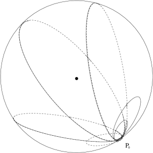
Without loss of generality, choose the base point to be on the equator, corresponding to the loop , as in Figure 7.
Starting at , the phase factor traces out a continuous curve until it reaches . Then one makes a patching transformation and goes over to . From onwards this again traces out a continuous curve ending in 1 for . In order that the curve so traced out winds round only half way in while being a closed curve in we must have
So the holonomy of the closed loop in corresponding to the flat connection is , which is the monopole charge.
5 Action principle and symmetry breaking
So far we have not discussed dynamics at all, that is, nothing much is said about the time evolution of the gauge system. These are given, in the classical and first quantized cases, by equations of motion, wich are normally obtained by the first variation of the functionals of the fields called actions. Various actions will describe various physical systems. We shall study some of them.
5.1 Maxwell equations and minimal coupling
The Maxwell action is usually given as:
This is the free field action, that is, it corresponds to a freely propagating electromagnetic field.
Recall that . Then
Varying with respect to we get
This, we recall, is the first pair of Maxwell’s vacuum equations in covariant notation. The second pair, in this situation, can be considered as kinematics, because by the definition of it is an identity:
or equivalently
with .
On the other hand, if we have a free (classical) particle in free space, then we define its free action
where is the proper time, the integral is along the worldline of the particle, with . Varying with respect to the worldline , we get
If we simply add the two actions together, we will not of course get any interaction. One way to introduce interaction is to add an “interaction term”, using the minimal coupling assumption:
So we have the total action:
Varying with respect to and we get
The first is Maxwell’s equation in the presence of an electric current-density , and the second is the Lorentz equation for a charge moving in an electromagnetic field.
For the quantum particle, which we assume to be a Dirac particle (i.e. with spin ), then we replace the particle action by
and the interaction term by
which on variation with respect to and give the following equations of motion:
These are then the quantum equations, the second being the well-known Dirac equation.
5.2 Yang–Mills equation
We can do the same for Yang–Mills theory.
In the free theory, we have the same action:
where now As before, varying with respect to we get the equations of motion, this time the Yang–Mills equation:
Here the covariant derivative is .
Again, in the presence of a colour electrically charged Dirac particle (a ‘quark’ for example), one can introduce an interaction term by the hypothesis of minimal coupling:
We obtain equations which are the analogues of the abelian ones:
Classical analogues, called the Wong equations, exist but since in applications particles are quantum, we shall not derive them here.
5.3 Wu–Yang criterion
What about the dynamics of monopoles? Let us go back to the abelian theory first. We know that in the presence of a magnetic monopole, the potential has to be patched, say by overlapping northern and southern hemispheres on any sphere surrounding the monopole. We immediately face several difficulties.
-
(a)
Varying patched ;
-
(b)
As the monopole moves, the patching moves with it, thus depending on say ;
-
(c)
What is the interaction term?
Wu–Yang criterion:
Equations of motion are obtained by varying the free field and free particle action, under the constraint that there exists a magnetic monopole. In other words, the interaction comes from the constraint. Intuitively, this is quite reasonable. Around the monopole, the field configurations have to be such that we have a nontrivial bundle. As the monopole moves in spacetime, the field configurations have to rearrange themselves to maintain this topological condition, hence there is mutual influence, that is, interaction.
So the prescription is:
to be varied under the constraint:
where we can insert either the classical or the quantum expression for the current.
Using the method of Lagrange multipliers, we in fact vary the auxiliary action:
The next question is, what are the variables? If we use , we still have the troubles (a) and (b). To answer this, let us look at the simpler problem of pure electromagnetism.
Previously, to get the free Maxwell equations we varied with respect to . Now we could also have varied with respect to , provided we compensate for the fact that there are more than , the former with 6 degrees of freedom and the latter with 4. Suppose now we restrict ourselves only to those satisfying , then we shall be able to recover (at least in a local region). This is clear in the language of forms, because
and in flat spacetime the Poincaré lemma will tell us that there exist a 1-form such that . So in other words, the sets of variables and are entirely equivalent. So suppose we form the action
and vary with respect to , we shall indeed get from
giving
which is the desired Maxwell’s equation.
So we see that the two derivations are entirely equivalent.
Coming back to the point monopole, the constraint is
We see that away from the monopole worldline, we have again
Along the monopole worldline, we know already that no exists. Hence in the constrained action principle, we are justified in using as variables. Hence the Wu–Yang criterion gives us the dynamics as follows:
These are identical to the dual of the equations of motion of an electrically charged particle, as expected—we shall study electromagnetic duality in more details later on.
What about nonabelian theory? In principle, the Wu–Yang criterion can be applied to nonabelian monopoles. In fact, it looks highly plausible that it can be applied to any topological charges to find their dynamics. The difficulty in the case of the nonabelian monopole is to write down the constraint. Recall the charge is defined as an element of .
This programme has in fact been carried out using loop space variables. Since Yang–Mills theory is not symmetric under the Hodge star ∗ (as we shall show) the equations thus obtained are new. Unfortunately it is a bit too lengthy to present here. What I shall do is to indicate to you how to use the Wu–Yang criterion in the pure Yang–Mills case to re-obtain the Yang–Mills equation, just as I did above for the Maxwell case.
Recall the constraint for the existence of , in terms of loop variables is that the ‘connection’
is flat, that is, its ‘curvature’ vanishes:
Next we want to write the Yang–Mills action in loop variables. It turns out that, modulo uncertainties about measures in function spaces,
where is an infinite normalization factor, the explicit expression for which need not bother us here.
So by the Wu–Yang criterion we form the constrained action with the Lagrange multipliers :
Because is skew, we can choose without loss of generality to be skew as well. Varying with respect to we get
Write this as a loop covariant derivative
Then
But and the commutator term vanishes, from which we obtain
This we refer to as the Polyakov equation, and is shown by Polyakov [AM Polyakov: Nucl. Phys. B164 (1980) 171–188] to be equivalent to Yang–Mills equation:
So we see that again the Wu–Yang criterion gives us the right dynamics.
Note. We have used the Wu-Yang criterion quite extensively, and have recovered all the known equations for interaction between the gauge field and charges, and have also obtained some new equations as well, notably for the nonabelian monopoles.
5.4 Symmetry breaking
From Lecture 2 we learned that we need to consider more complicated gauge theories, that is, those that exhibit symmetry breaking as in electroweak theory.
We shall now look at the action for electroweak theory. For simplicity and to make the symmetry breaking mechanism more transparent, we shall omit the charges (i.e. leptons).
To the Yang–Mills action we now add the Higgs action:
where is an doublet of complex scalar fields
with weak hypercharge . Hence the covariant derivative is
where represents the 3 components of the weak isospin gauge potential, and the weak hypercharge potential, and and the corresponding coupling constants. The potential is
If , then the scalar field has mass and the vacuum (or ground state) corresponds to . If , we get the famous Mexican hat potential, and the vacuum (with minimum) is given by
We now choose a gauge such that
In this way, the vacuum corresponds to a particular direction in the space of and once this choice is made, the physics will no longer be invariant under the whole of the group. This is symmetry breaking. In fact, since is a complex vector in (although we sometimes call it a spinor), there will be a phase rotation left over after fixing a directin as above, and this constitutes the ‘little group’ corresponding to electromagnetism.
For a quantum field theory, we look at quantum excitations around the vacuum, that is,
where , which is a gauge choice. Hence
from which
Now define:
with
or in terms of the Weinberg angle
we have
As far as the particle spectrum is concerned, cubic and quartic terms are unimportant. They can be either got rid of by redefining fields or they represent self-interactions. So we concentrate on the quadratic terms.
Recall the Klein–Gordon Lagrangian
(after integration by parts). So from the previous expression for plus the Yang–Mills action, we see that the following fields acquire a nonzero mass term, giving
(and also the Higgs field becomes massive) while the abelian vector field
has no mass term and hence remains massless. This can easily be identified as the photon (especially if we consider the lepton terms as well).
6 Electric–magnetic duality
Electric–magnetic duality, where it exists, is an important concept in theoretical physics.
-
1.
As a symmetry of nature, we should study it. Also since it is discrete, it should be relatively easy.
-
2.
As a result of this symmetry we need study only half of the phenomena.
-
3.
Dirac’s quantization condition (abelian and nonabelian respectively) says
This should hold even under renormalization. We have therefore a correspondence which relates weak coupling (where perturbation expansion is good) to strong coupling (where perturbation expansion is bad).
-
4.
’t Hooft’s theorem (see later) leads to a mechanism for confinement (of quarks) via duality.
6.1 Abelian theory
We recall that the duality operator (∗) is defined by:
the sign being the consequence of Minkowski signature .
Duality, as the name implies, is such that we recover the original field tensor (up to sign) if we do the operation twice:
In terms of the electric field and the magnetic field these tensors can be represented in matrix form:
So we see that under
The question is: is the theory invariant under this duality?
In vacuo, the Maxwell equations are:
Hence we conclude that the theory is indeed invariant in this case.
But we can go back even further and see that the derivation of these equations is also invariant. In this connection we note that
so that the action is invariant (the sign being of no significance as it does not affect the dynamics). Applying the Wu–Yang criterion, we can use either (1) or (2) as constraint and obtain the other as equation of motion, so that we end up with the same equations in both cases.
Recall that
leading to
which implies
This is clear by looking at Chart 6.6, both columns 2 and 3.
Next, in the presence of a magnetic monopole, we have:
-
(1)
-
(2)
.
If we now look at Chart 6.6, column 1 or 2, we see that:
(2) as constraint (1) as equation of motion.
Dually, in the presence of an electric charge, we have
-
(1)
-
(2)
.
And now Chart 6.6, column 3 or 4, tells us:
(1) as constraint (2) as equation of motion.
Remarks
-
1.
Duality: . In other words, the duality links charges monopoles, and which is which depends on which are the fields/potentials.
-
2.
A dual potential emerges, which is just the Lagrange multiplier. Away from charges and monopoles, we have both and . In pure theory, neither nor appears in the equations, but in the presence of charges/monopoles, the Lagrange multiplers cannot be eliminated and the potentials appear explicitly, as demanded by the Bohm–Aharonov experiment.
-
3.
The duality goes deeper, as linking physics with geometry.
Dually, we have exactly the same picture:
6.2 The star operation in Yang–Mills theory
In nonabelian theory, we have the same star operation:
Let us now try to fill in the boxes as in the abelian case. We find in the direct picture:
And in the dual picture:
All these go to show that the star operation in nonabelian theory does not give us the desired electric–magnetic duality, unlike the abelian case. In fact, we have a stronger result, in the following counter-example discovered by Gu and Yang.
The Gu–Yang counter-example
Gu and Yang phrase their example in terms of , but we can equally think in terms of . Since in general , there is really no reason to suppose that is in any sense exact. Furthermore, we are not asking to be exact, but we want the existence of for which . So the existence of a gauge potential in nonabelian theory has very little to do with the usual Poincaré lemma.
Counter-example. Let . Take an explicit ‘hedgehog potential’
(abandoning our summation convention temporarily) with a function of the radius satisfying
It can easily be verified that for such a potential the gauge field satisfies the Yang–Mills source-free equation:
Previously, Wu and Yang found numerical solutions to the above differential equation for , depending on a real parameter , with
Now let
and consider as 3 vectors in 3-space. Then it can be proved that
Hence for the given solution, the vectors are linearly independent.
Suppose for a contradiction that exists as a potential for . Then its Bianchi identity is
This, together with the Yang–Mills source-free equation, implies
where for convenience we have absorbed the coupling constant into , into . Notice that may not be zero, but it does not contribute because .
Write now . Then in 3-space notation, the commutator equation can be written as:
We now claim that:
In fact, all the quadruples etc. are coplanar. This implies, say,
which in turn implies
Hence
and therefore all are equal, say to . This gives
which justifies our claim.
We therefore conclude:
Now
but on the other hand
which is a contradiction.
Claim. Hence nonabelian Yang–Mills theory is not dual symmetric under ∗.
-
1.
need not exist,
-
2.
the dual of Yang-Mills equation is not Bianchi identity.
6.3 Generalized electric–magnetic dualtiy for Yang–Mills theory
We saw that electromagnetic duality in Maxwell theory is both important and useful. So we want to salvage the situation as regards to nonabelian theory. There are two ways of going about it.
-
(A)
Generalize the concept of duality, that is, modify it in the nonabelian case.
-
(B)
Enrich the theory, for example, make it supersymmetric, so as to enlarge existing symmetries.
We shall briefly talk about both. Take (A) first. We seek a dual transform satisfying the following properties:
-
1.
,
-
2.
electric field magnetic fields ,
-
3.
both and exist as potentials (away from charges),
-
4.
magnetic charges are monopoles of , and electric charges are monopoles of ,
-
5.
reduces to ∗ in the abelian case.
So far, we are only able to express this new dual transform in terms of loop variables. I cannot go through the construction here but those interested can refer to our papers, especially recent reviews. Suffice it to say that the above 5 points are indeed satisfied, and we have full duality as depicted below:
Dually, we have
6.4 ’t Hooft’s theorem and its consequences
In a quantum gauge field theory, the phase factor
is an operator in a Hilbert space. Let
which is still an operator. This is the more usual definition of the Wilson loop.
In a gauge theory with gauge group corresponding to the Lie algebra , ’t Hooft introduced abstractly the operator dual to , by the commutation relation
where is the linking number between the two spatial loops and . He describes these two quantities as:
-
•
measures the magnetic flux through and creates electric flux along
-
•
measures the electric flux through and creates magnetic flux along
So they play dual roles in the sense we have been considering. However, there was no “magnetic” potential available at the time, so that the definition of was not explicit, only through the commutation relation above.
But in the construction mentioned in the last subsection (which I did not give explicitly), the magnetic potential exists, so that one can actually prove the commutation relation. This has been done about 2 years ago.
’t Hooft’s Theorem. If the Wilson loop operator of an theory and its dual theory satisfy the commutation relation given above, then:
Note that the second statement follows from the first, given that the operation of duality is its own inverse (up to sign).
The theorem does not hold for a theory, where both and may exist in a Coulomb phase, that is, with long range potential ().
The statement is phrased in terms of phase transition, and has profound implications. It has been a cornerstone for attempts to prove quark confinement ever since.
I may add that we have exploited ’t Hooft’s theorem in the reverse way. Given that colour is confined, we deduce that dual colour is broken, which we have identified as the 3 generations of particles as observed in nature. There are many consequences of such a hypothesis, not only in particle physics, but also in nuclear and astrophysics.
Coming back to the commutation relation, I wish to show you how to prove it in the abelian case, just to give you a taste of what is involved. The nonabelian case is too complicated to treat here.
In the abelian case, we do not need the trace, hence , and the are genuine exponentials. So if we can show the following relation for the exponents, we shall have proved the required commutation relation:
Using Stokes’ theorem the second integral
For simplicity, suppose the linking number . Then the loop will intersect at some point —if it intersects more than once, the other contributions will cancel in pairs, so we shall ignore them. So except for , all points in are spatially separated from points on .
Using the canonical commutation relation for and
we get
by Dirac’s quantization condition.
Hence we have shown explicitly in the abelian case that our definition of duality coincides with ’t Hooft’s. The same is true in the nonabelian case.
6.5 Magnetic monopoles from symmetry breaking
We looked at electroweak symmetry breaking in detail: . We can also do similar breaking with . Again we can choose the Higgs field in the direction, and the residual symmetry will again be a , this time generated by the generator .
Now being simply connected, there are no nontrivial bundles over . However, there can be nontrivial reductions to the subgroup. Topologically, this can be seen by looking at part of the exact sequence of homotopy groups, obtained from the principal bundle:
whence
The boundary condition of the Higgs field at infinity will determine the nature of the reduced bundle (more precisely, its first Chern class), that is, the homotopy class of the map: , the first being the sphere at infinity. This is precisely given by , which by the exactness of the above, is isomorphic to the magnetic charges of the residual , namely .
Let us look at an example, the residual charge 1 magnetic monopole. It is a particular solution of the Yang–Mills–Higgs equations we saw before.
Inserting the asymptotic condition we get a solution, for large , similar to the Wu–Yang potential we had:
that is, a magnetic field in radial direction at infinity, which is why this is referred to by Polyakov as the “hedgehog solution”. Such a solution is called a ’t Hooft–Polyakov monopole.
In the (unphysical) limit studied by Prasad and Summerfield,
exact solutions exist for . These are finite energy solitonic solutions.
There is a parameter occurring in the behaviour of , which represents the mass of the soliton, and it satisfies an inequality given by Bogomolny. If this bound is saturated, then we have what is known as a BPS monopole. These have been much studied because they can be obtained by a process called dimensional reduction from instanton solutions of 4-dimensional Euclidean self-dual Yang–Mills equations, as the gauge fields being static have only spatial components, leaving the (imaginary) temporal component of the instanton to play the role of the Higgs field.
Also these have been extended to exhibit electric charges as well. The resulting extended ‘particle’ is then a dyon: carrying both electric and magnetic charges.
6.6 Seiberg–Witten duality
The second way to study electric-magneitc duality is to exploit the duality between the electric and magnetic charges which occurs as a result of symmetry breaking from a nonabelian Yang–Mills theory.
In the models so far studied, supersymmetry is a necessary ingredient. Supersummetry is a hypothetical symmetry between fermions and bosons, and has tremendous theoretical and mathematical appeal to a lot of physicists. We cannot discuss it here for lack of time (and expertise!). The dual symmetry I shall outline below works for all and some supersymmetric Yang–Mills theories, with gauge group —this can be generalized.
The bosonic part of the action is
where the last term corresponds to the second Chern class or instanton number. This is a topological term, and the coefficient in front of it is the so-called -vacuum angle. Experimentally it is very nearly 0.
By giving a nonzero vacuum expectation value to the Higgs field , we effect the symmetry breaking . There are solutions which are BPS monopoles. In fact they are dyons, with both electric and magnetic charges. Their masses satisfy the Bogomolny bound:
where
One sees that the mass formula is invariant under
so that this theory of charges and monopoles are invariant under the group .
In the particular case when , the generator of corresponding to , that is , induces
and we recover the usual electric-magnetic dualtiy with . This also goes under the name of -duality.
Explicit solutions are constructed by making use of a certain holomorphic function of occurring in the theory having to do with the metric on the moduli space. This duality is found to be a symmetry of the quantum field theory.
Seibery and Witten also considered supersymmetric Yang–Mills theories in which the dual symmetry is only partial, in the sense that the spectrum of dyons in one theory is found to match the dual spectrum (electric magnetic) of another theory, perhaps with a different gauge group.
The whole subject has been intensely studied in recent years, with many ramifications into string theory, membrane theory and -theory. They are definitely outside the scope of these lectures.
![[Uncaptioned image]](/html/hep-th/0006178/assets/x7.png)
Pure Electromagnetism.
![[Uncaptioned image]](/html/hep-th/0006178/assets/x8.png)
Electromagnetism with charges.
Bibliography
General Gauge theory
-
•
IJR Aitchison and AJG Hey, Gauge Theories in Particle Physics, Adam Hilger, 2nd edition, 1989.
-
•
AP Balachandran et al., Gauge Symmetries and Fibre Bundles, Lecture Notes in Physics # 188, Springer, Berlin, 1983.
-
•
Chan Hong-Mo and Tsou Sheung Tsun, Elementary Gauge Theory Concepts, World Scientific, Singapore, 1993.
-
•
Tsou Sheung Tsun, Symmetry and symmetry breaking in particle physics, in Proc. 8th EWM General Meeting, Trieste 1997, hep-th/9803159.
-
•
TT Wu and CN Yang, Concepts of nonintegrable phase factors and global formulation of gauge fields, Phys. Rev. D12 (1975) 3845–3857.
Mathematics background
-
•
N. Steenrod, The topology of fibre bundles, Princeton University Press, Princeton, 1974.
-
•
S. Kobayashi and K. Nomizu, Foundations of Differential Geometry, Vol. I, Interscience, New York, 1963.
Further interests
Those who are interested in our recent work on duality may like to read:
-
•
Chan Hong-Mo and Tsou Sheung Tsun, Nonabelian Generalization of Electric–Magnetic Duality—A Brief Review, hep-th/9904102, RAL-TR-1999-014, invited review paper, International J. Mod. Phys. A14 (1999) 2139–2172.
-
•
Chan Hong-Mo and Tsou Sheung Tsun, The Dualized Standard Model and its Applications—an Interim Report, hep-ph/9904406, RAL-TR-1999-015, invited review paper, International J. Mod. Phys. A14 (1999) 2173–2203.