CERN-TH/2000-118

KUL-TF-2000/15

CITA-2000-12

hep-th/0006179

Superconformal Symmetry, Supergravity and Cosmology

Renata Kallosh,^1,† Lev Kofman,²
Andrei Linde,^1,† and Antoine Van Proeyen ^3,‡

¹ Theory Division, CERN, CH-1211 Genève 23, Switzerland
² CITA, University of Toronto, 60 St George Str, Toronto, ON M5S 3H8, Canada
³ Instituut voor Theoretische Fysica, Katholieke Universiteit Leuven,
Celestijnenlaan 200D B-3001 Leuven, Belgium

Abstract

We introduce the general $N=1$ gauge theory superconformally coupled to supergravity. The theory has local $SU(2,2|1)$ symmetry and no dimensional parameters. The superconformal origin of the Fayet–Iliopoulos (FI) terms is clarified. The phase of this theory with spontaneously broken conformal symmetry gives various formulations of $N=1$ supergravity interacting with matter, depending on the choice of the $R$-symmetry fixing.

We have found that the locally superconformal theory is useful for describing the physics of the early universe with a conformally flat FRW metric. Few applications of superconformal theory to cosmology include the study of i) particle production after inflation, particularly the nonconformal helicity-${\textstyle\frac{1}{2}}$ states of gravitino, ii) the super-Higgs effect in cosmology and the derivation of the equations for the gravitino interacting with any number of chiral and vector multiplets in the gravitational background with varying scalar fields, iii) the weak-coupling limit of supergravity $M_{P}\rightarrow\infty$ and gravitino–goldstino equivalence. This explains why gravitino production in the early universe is not suppressed in the limit of weak gravitational coupling.

We discuss the possible existence of an unbroken phase of the superconformal theories, interpreted as a strong-coupling limit of supergravity $M_{P}\rightarrow 0$.

 ^† On leave of absence from Stanford University until 1 September 2000
^‡ Onderzoeksdirecteur, FWO, Belgium

1 Introduction

Over the last few years M-theory and string theory have focused mainly on the superconformal theories and adS/CFT (anti-de Sitter/conformal field theory) correspondence [1]. In particular, IIB string theory on $adS_{5}\times S^{5}$ is related to $SU(2,2|4)$ superconformal symmetry. The relation between various anti-de Sitter compactifications of M-theory and string theory and the relevant superconformal symmetries were described in detail in [2]. In particular, one finds the $SU(2,2|1)$ superconformal algebra from the anti-de Sitter compactification of the string theory with ${1\over 4}$ of the unbroken supersymmetry. These recent developments in M-theory and non-perturbative string theory suggest that we should take a fresh look at the superconformal formulation underlying the supergravity. One of the basic features of superconformal theory is that generically it treats the gravitational coupling $M_{P}^{2}=\kappa^{-2}$ as some function of a set of scalars $\kappa^{-2}\Rightarrow-{\textstyle\frac{1}{3}}{\cal N}(X,\bar{X})$, just like in string theory the string coupling is given by a dilaton field, $g_{s}^{-2}={\rm e}^{\phi}$. In the superconformal action the term ${\textstyle\frac{1}{6}}{\cal N}(X,\bar{X})R$ replaces the standard Einstein term $-{\textstyle\frac{1}{2}}M_{P}^{2}R$ of supergravity.

The function of scalars, ${\cal N}(X,\bar{X})$, codifies the Kähler potential. When the theory is in a Higgs phase, $-{\textstyle\frac{1}{3}}{\cal N}(X,\bar{X})=M_{P}^{2}+f(X,\bar{X})$ and the function $f(X,\bar{X})$ can be gauged away using local conformal symmetry: the superconformal symmetry is broken spontaneously and supergravity with the dimensional parameter $M_{P}$ is recovered.

In addition to the state with the spontaneously broken superconformal symmetry, one may also speculate about the unbroken phase of the superconformal theory where the function ${\cal N}(X,\bar{X})$ has a vanishing vacuum expectation value and there are no dimensional parameters in the theory. This phase of the superconformal theory can be considered as the strong-coupling limit of supergravity $M_{P}^{2}\to 0$. In such a limit the theory may be completely different from classical supergravity, which represents the weak-coupling limit of the Higgs phase of the superconformal theory. Even though we do not have a clear constructive approach to this phase of the theory at the moment, we do have some distinct examples of the configurations, analogous to cosmic strings, where at the core of the string ${\cal N}(X,\bar{X})=0$. We consider this as an indication that the superconformal theory, in addition to the Higgs phase where it is equivalent to supergravity, may have an unbroken phase related to the strong-coupling limit of supergravity.

At present the low-energy phenomenology is described by $N=1$, $d=4$ supergravity [3, 4, 5, 6]. Some preferable choices of the Kähler  potentials, superpotentials and Yang–Mills couplings hopefully will be selected at the level of the fundamental theory. Until the fundamental theory of all interactions is well understood, one may try to address the issues of particle physics and cosmology in the context of the most general phenomenological $N=1$ supergravity–Yang–Mills–matter theory [6]. This, in fact, has been the case over the last almost 20 years. One can find the Lagrangian describing this theory in many textbooks and review papers [7, 8, 9, 10, 11].

The phenomenological $N=1$ supergravity–Yang–Mills–matter theory was derived in [6, 12] using local $SU(2,2|1)$ superconformal symmetry only as a tool, within the framework of [13, 14, 15]. The transition from the superconformal supergravity to the usual Poincaré supergravity occurs after the conformal compensator field (which we will call the conformon) becomes fixed. Until very recently, the opinion was that the only role of superconformal theory is to provide the tensor calculus to derive supergravity, and that this theory has no interesting physics in it. Therefore, the textbook description of the phenomenological $N=1$ supergravity–Yang–Mills–matter theory [8, 9, 10, 11], with the notable exception of [7], practically skips the superconformal formulation of this theory.

$N=2$ supergravity–Yang–Mills–matter theory with special geometry [16, 17, 18] was constructed later than the $N=1$ theory. This theory has been used extensively during recent years, in particular with application to BPS black holes [19]. It is associated with low-energy string theory compactified on Calabi–Yau manifolds, and instead of functions one has to define sections of appropriate line bundles over the Kähler  manifold. This construction has various advantages, in particular it treats all scalars in the superconformal version of the theory on an equal footing. This means that there is no distinction between the physical scalars and the conformal compensator scalar before gauge-fixing of conformal symmetry is performed. All available formulations of $N=1$ theory make a particular choice for the compensator even before conformal symmetry is gauge-fixed [6, 12, 20]. We will find that some features of $N=2$ theory may be implemented into $N=1$ theory, which may eventually lead to a better understanding of this theory. In fact, only very recently the power of superconformal pre-Poincaré $N=2$ supergravity was demonstrated in calculations of quantum corrections to the supersymmetric black hole entropy [21].

The first purpose of this paper is to present a detailed derivation of $SU(2,2|1)$-symmetric superconformal theory. In previous derivations [6, 12], where it was only a tool, some part of the $SU(2,2|1)$ symmetry was broken at an early stage. We will first present the action with full superconformal symmetry before explicitly indicating how we gauge-fix the dilations, $R$-symmetry and $S$-supersymmetry, leading to Poincaré supergravity.

This formulation of the theory has several advantages. For example, it simultaneously incorporates two different formulations of phenomenological supergravity depending on the gauge-fixing of the $R$-symmetry. The first formulation, which is more standard, corresponds to [6], where the Lagrangian depends not on two functions, the Kähler potential ${\cal K}(z,z^{*})$ and the superpotential $W(z)$, but only on one combination ${\cal G}(z,z^{*})=-{\cal K}(z,z^{*})-\ln|M_{P}^{-3}W|^{2}$ and has real fermion mass terms. The other one, closer to [9, 10], has a non-singular dependence on the superpotential $W$, but complex fermion masses in general. It is important to have both versions of the theory under control, especially in situations where the superpotential $W(z)$ may vanish, which often happens in cosmological applications.

The new formulation will allow us to give a detailed explanation of the superconformal origin of Fayet–Iliopoulos (FI) terms by including gauge transformations of the conformon field as first suggested in [20].

In addition to providing a new perspective on the old problems of supergravity, the superconformal formulation appears to be most suitable one for investigation of cosmology. Indeed, the Friedmann–Robertson–Walker (FRW) universe is conformally flat. This means, in particular, that the metric of an FRW universe can be transformed into the form $\rm{d}s^{2}=a^{2}(\eta)(\rm{d}\eta^{2}-\rm{d}x^{2})$, where $\eta$ is conformal time, $a(\eta)$ is the scale factor of the universe. If the theory is conformally invariant, then the scale factor $a(\eta)$ can be absorbed into a redefinition of the metric and fields. These redefined fields do not depend on $a(\eta)$, so the theory of particles in an expanding curved universe reduces to a much simpler theory in a fixed flat Minkowski space. This considerably simplifies the investigation of the behaviour of particles and fields during the expansion of the universe. Ideally, one may perform the investigation of all processes in the early universe within the framework of superconformal theory, where expansion of the universe does not show up, and then one may switch to the standard formulation with the fixed Planck mass at the very end of the calculations. This is a new and very exciting possibility; it would be hard to anticipate this possibility by looking at the lengthy and extremely complicated Lagrangian of phenomenological supergravity which appears after the breaking of the superconformal invariance of the original theory.

In the beginning of our investigation we did not fully recognize this possibility. We were working within the traditional framework of phenomenological supergravity, making only occasional use of the underlying superconformal invariance. Therefore, we were quite surprised when we realized that in order to obtain some of our results it was necessary to make certain field redefinitions in phenomenological supergravity, which eventually brought us back to the original superconformal formulation.

One of the problems that we were trying to address, was the issue of conformal invariance of the gravitino and the possibility of non-thermal gravitino production in the early universe.

Many observable properties of the universe are to a large extent determined by the underlying conformal properties of the fields. One may consider inflaton scalar field(s) $\phi$ which drive inflation, inflaton fluctuations which generate cosmological metric fluctuations, gravitational waves generated during inflation, photons in the cosmic microwave background (CMB) radiation which propagate (almost) freely from the last scattering surface, etc. If the conformal properties of any of these fields were different, the universe would look quite different too. For example, the theory of the usual massless electromagnetic field is conformally invariant. This implies, in particular, that the strength of the magnetic field in the universe decreases as $a^{-2}(\eta)$. As a result, all vector fields become exponentially small after inflation. Meanwhile the theory of the inflaton field(s) should not be conformally invariant, because otherwise these fields would rapidly disappear and inflation would never happen.

Superconformal supergravity is particularly suitable for studying the conformal properties of various fields, because within this framework all fields initially are conformally covariant; this invariance becomes spontaneously broken only when one uses the gauge $-{\textstyle\frac{1}{3}}{\cal N}(X,\bar{X})=M_{P}^{2}$.

The issue of conformal invariance of the gravitino remained rather obscure for a long time. One could argue that a massless gravitino should be conformally invariant. Once we introduce the scalar field driving inflation, the gravitino acquires a mass $m_{3/2}={\rm e}^{{\cal K}/2}|W|/M_{P}^{2}$. Thus, one could expect that conformal invariance of gravitino equations should be broken only by the small gravitino mass $m_{3/2}$, which is suppressed by the small gravitational coupling constant $M_{P}^{-2}$. This is indeed the case for the gravitino component with helicity $\pm{\textstyle\frac{3}{2}}$. However, breaking of conformal invariance for the gravitino component with helicity $\pm{\textstyle\frac{1}{2}}$, which appears due to the super-Higgs effect, is much stronger. In the first approximation in the weak gravitational coupling, it is related to the chiral fermion mass scale [22].

The difference between the two gravitino components becomes especially important when one studies gravitino production after inflation. It is usually assumed that gravitinos have mass $m_{3/2}\sim 10^{2}$–$10^{3}$ GeV. Such particles decay very late, which leads to disasterous cosmological consequences unless the ratio of their number density $n_{3/2}$ to the entropy density $s$ is extremely small. In particular, the ratio $n_{3/2}/s$ should be smaller than ${\rm O}(10^{-15})$ for gravitinos with mass ${\rm O}(100)$ GeV [23, 24].

The standard thermal mechanism of gravitino production involves scattering of particles at high temperature in the early universe. To avoid excessive production of gravitinos one must assume that the reheating temperature of the universe after inflation was smaller than $10^{8}$–$10^{9}$ GeV [23, 24].

However, gravitinos can also be produced during the oscillations of the inflaton field at the end of inflation. The theory of the production of the gravitino with helicity $\pm{\textstyle\frac{3}{2}}$ is relatively straightforward, and the effect typically is not very large, because it appears mainly due to the non-adiabatic change of the small gravitino mass during the scalar field oscillations and the expansion of the universe [25, 26]. This effect disappears in the limit of the small gravitational coupling, $M_{P}\to\infty$.

One could expect that the same should happen for the gravitinos with helicity $\pm{\textstyle\frac{1}{2}}$. However, we have found, in models with one chiral multiplet, that the gravitinos with helicity $\pm{\textstyle\frac{1}{2}}$ can be produced as abundantly as normal matter particles not belonging to the gravitational multiplet, i.e. the rate of their production does not vanish in the limit $M_{P}\to\infty$ [22].

More exactly, we have found that if one considers the underlying globally supersymmetric theory with one chiral multiplet, then the chiral fermion $\chi$ has mass $W_{,\phi\phi}={\partial^{2}W\over\partial\phi^{2}}$, where $\phi=zM_{P}$. This mass oscillates during the oscillations of the scalar field $\phi$, which would lead to production of fermions $\chi$ in the globally supersymmetric theory. In supergravity, these fermions enter the definition of goldstinos, which are eaten by gravitinos and give rise to the gravitino component with helicity $\pm{\textstyle\frac{1}{2}}$. This is the deep reason why, as we have found, the probability of production of the helicity-${\textstyle\frac{1}{2}}$ gravitinos does not vanish in the limit $M_{P}\to\infty$ and coincides with the probability of the production of the chiral fermions $\chi$ (and, correspondingly, of the goldstino production) in the underlying globally supersymmetric theory [22]. This surprising result was confirmed in the paper by Giudice, Tkachev and Riotto [27], and in subsequent papers by several other authors [28]–[33].

However, until now a complete supergravity treatment of the gravitino production was achieved only for models with one chiral multiplet. Even in this case the theory of gravitino production was very complicated, and it was not quite clear how one could study the realistic models with many chiral and vector multiplets.

One of the ideas was to use the gravitino–goldstino correspondence in the hope that the leading effect can be found by the relatively simple investigation of production of goldstinos in a globally supersymmetric theory, instead of a direct investigation of the gravitino production. Indeed, this idea worked well for the case of one multiplet [22, 27, 31], but there was no proof that the same method will apply in the general case as well.

Equations for the goldstino in the theory without vector multiplets but with any number of chiral multiplets were derived in [30] within the framework of globally supersymmetric theories, neglecting expansion of the universe. The hope was expressed that the gravitino–goldstino equivalence theorem [34, 35] will justify such derivation as representing the equation for the helicity $\pm{\textstyle\frac{1}{2}}$ of the gravitino in the limit of $M_{P}\rightarrow\infty$ in supergravity.

However, the relevance of the equivalence theorem for scattering amplitudes in the high-energy limit [34, 35] to the problem of gravitino production by the oscillating scalar field in a cosmological background in the theory with many chiral and vector multiplets was not quite obvious. In fact, one did not even have a clear picture of the super-Higgs effect in cosmology, which was essential for the understanding of the goldstino–gravitino correspondence, and it was rather non-trivial to give a precise definition of what we mean by the gravitino interactions in the limit $M_{P}\rightarrow\infty$.

As we will see, the concept of the goldstino in the background with time-dependent metric and scalars, and the proper definition of the $M_{P}\rightarrow\infty$ limit of supergravity is greatly simplified in the context of the superconformal theory. It turned out that the original fields of the superconformal theory rather than the fields used in phenomenological supergravity are those which should be held fixed in this limit.

Therefore, after deriving two versions of standard supergravity, before starting with gravitino equations, we will perform specific modifications of the theory so that the basic fields will again be those of superconformal theory. This includes, in particular, a number of rescalings. All of them have one simple purpose: to use as basic variables the fields of the underlying superconformal theory. This form of supergravity is suitable for considering the limit in which gravity decouples and a globally supersymmetric theory appears.

These modifications of the usual supergravity will allow us to achieve the second purpose of this paper: to generalize the super-Higgs effect for cosmology, and to derive the gravitino field equations in the theory with any number of chiral and vector multiplets.

In Minkowski space, the supersymmetry breaking and super-Higgs effect occur only if the gravitino has non-vanishing mass $m_{3/2}={\rm e}^{{\cal K}/2}|W|/M_{P}^{2}$, because the generator of the supersymmetry transformations is proportional to $m_{3/2}^{2}$. This parameter depends on $\phi$, so it changes during the oscillations of the scalar field $\phi$, and it may vanish at some stages of the evolution of the universe. However, we will show that the criterion for supersymmetry breaking and the existence of the super-Higgs effect in the post-inflationary universe with the energy density provided by the scalar field is not $m_{3/2}^{2}\not=0$, but rather $H^{2}+m_{3/2}^{2}\not=0$. This criterion is always satisfied, so that the super-Higgs effect will always take place in a universe with the energy density dominated by the scalar fields. This is an important conclusion that will allow us to use the unitary gauge, in which the goldstino is eaten by the gravitino throughout our calculations.

The system of equations for the gravitino in the theory with many chiral and vector multiplets is rather complicated. However, they will be given in a form in which the limit $M_{P}\rightarrow\infty$ can be taken straightforwardly. This will clarify the status of the gravitino–goldstino equivalence theorem in the limit $M_{P}\rightarrow\infty$ and the relation of supergravity to the globally supersymmetric theories. The difference with [34, 35] is that we will not be working with the $S$-matrix elements in the flat background, but with classical equations for bosons and fermions in the cosmological setting. We will therefore not compare the matrix elements, but the form of the highly nonlinear field equations, relevant for the production of particles in the early universe. This equivalence theorem will explain why the effect of non-thermal production of gravitinos in the early universe, in general, is not suppressed by the inverse powers of $M_{P}$.

This theorem should be used with care since its results are easy to misinterpret. It is very useful when the process of particle production occurs so fast that one can neglect expansion of the universe. However, in the theories with many chiral and vector multiplets, the definition of the goldstino gradually changes during the expansion of the universe. In the beginning, the goldstino is associated with a certain combination of chiral fermions, the superpartners of the scalar fields driving inflation (inflatino). In the end of the process, the goldstino may be associated with a completely different combination of chiral fermions. Therefore, one could argue that gravitino (inflatino) production in the very early universe may be irrelevant for the calculation of the final number of gravitinos produced, because all chiral fermions produced at the beginning of this process may not give any contribution to the goldstino eaten by the gravitino at the end of the process [36].

This issue turns out to be rather complicated. The goldstino–gravitino correspondence is a useful tool in regimes when the expansion of the universe can be neglected. However, in order to describe the change between different definitions of the goldstino due to the expansion of the universe one should go beyond the limit $M_{P}\to\infty$, which may invalidate the argument given above. In this case instead of using the equivalence theorem one should study gravitino equations in the unitary gauge. As we will see, in the epoch where the definition of goldstino changes because of the expansion of the universe, the number of gravitinos may also change because they can mix with other fermions. A detailed investigation is necessary in order to find out whether this leads to a depletion of the gravitinos produced at the first stages of the process, or, vice versa, to their additional production due to the non-adiabaticity related to the change of the nature of the goldstino.

In our paper we will develop the framework which can be used in order to address this question, as well as other questions related to the gravitino production. We will derive equations for the gravitino in theories with an arbitrary number of chiral and vector multiplets, and analyse some limiting cases where their solutions can be obtained.

The paper is organized as follows. In section 2 we give an example of the local conformally symmetric theory and introduce the concept of the conformon field. We use this example, in particular, to explain the conformal properties of the gravitino. We discuss the cosmic-string-type configuration of superconformal theory. There is an infinite gravitational coupling at the core of the string.

Section 3 presents the $SU(2,2|1)$ symmetric action of the Yang–Mills and chiral multiplets superconformally coupled to supergravity. In section 3.1, the conformal and chiral weights of all fields are organized in a table. The generic cosmic-string-type configurations with vanishing ${\cal N}$ at the core are discussed. The superconformal origin of the Kähler potential and superpotential is explained and the $S$- and $Q$-supersymmetry transformations of all fields are given. The auxiliary fields are eliminated on shell. We comment on the quantization in the case of topologically non-trivial Kähler manifolds. Section 3.2 explains the gauge-fixing of superfluous symmetries which leads to supergravity. In particular, the conformon field is gauge-fixed to give $M_{P}$. Here, as well as in appendix C, the origin of the Kähler geometry is clarified.

Section 4 is about the Yang–Mills part of the theory, showing that any gauged isometry can be obtained in the superconformal formulation by including transformations of the conformon multiplet. In section 4.1, Killing isometries, which act on all scalars of the theory, including the conformon field, are given. The Killing potentials, which encode the isometries, may include some constant parts related to the gauge symmetries of the conformon. This provides the superconformal origin of the Fayet–Iliopoulos terms ($D$-terms). The new mechanism of the generation of the FI terms is explained in section 4.2, and some examples are given.

Section 5 shows the derivation of the phenomenological Lagrangian. First, in section 5.1, the Kähler structure and the superpotential are derived from the superconformal structures. Section 5.2 gives a first discussion of the goldstino, which is still natural to do in the superconformal context. Section 5.3 presents the full phenomenological Lagrangian, where the $R$-symmetry of the local $SU(2,2|1)$ is still not gauge-fixed. The two possibilities of the gauge-fixing of this remaining $U(1)$ symmetry are explained in this section: either the Kähler symmetric gauge, or that which is non-singular when the superpotential is vanishing. Thus it is easy to obtain both theories from one action in (5.3). Finally, in section 5.4, we perform various rescalings of the fields of the theory in view of a rigid limit, which bring us back to the original fields from which the superconformal theory was build and which will be used in the rest of the paper.

Section 6 is dedicated to the gravitino. In section 6.1, the relevant part of the action is given which shows clearly the mixing between the gravitino, chiral fermions and gaugino. Field equations without specifying a gauge-fixing for local supersymmetry are derived in section 6.2. Section 6.3 offers a master gravitino field equation and the constraints. We discuss the choice of the unitary gauge where the goldstino vanishes in the case of the non-constant gravitational and scalar backgrounds.

In section 7 we develop our formalism in application to cosmology. We first specify the assumptions related to cosmology in section 7.1. Section 7.2 describes the super-Higgs effect in cosmology with time-dependent scalars and a conformally flat time-dependent metric. In section 7.3 the important constraints for the gravitino are given in the unitary gauge, where the goldstino vanishes. The system of equations for the gravitino interacting with other fermionic fields of the theory, chiral fermions as well as gauginos, is derived in section 7.4. In section 7.5 we give a useful second-order form of the equation for the helicity-$\pm{\textstyle\frac{1}{2}}$ gravitino interacting with other fermions.

Section 8 presents the goldstino–gravitino equivalence theorem explaining why the effect of the helicity-$\pm{\textstyle\frac{1}{2}}$ gravitino is not suppressed in the limit of large $M_{P}$.

In section 9 we consider the cases with one or two multiplets, and make a number of simplifications. Some parts of this section consider only real scalar fields. In other parts the limit of these equations at large $M_{P}$ is taken.

Section 10 is devoted to gravitino production after inflation. We give an overview of the previous investigation of the theories with one chiral multiplet, and then discuss various issues related to gravitino production in realistic models with several multiplets.

In the discussion section we give a short overview of the results.

Appendix A presents the notation, including a clarification of the rules of complex conjugation. The consequences of a conformal metric are reviewed in appendix B. Appendix C gives the steps needed to go from a conformal form of the action to the Kähler geometry. It is formulated such that it applies more generally than for $N=1$ theories. It also discusses the relation with Sasakian manifolds, and at the end gives the connection between the conformal chiral-covariant derivatives and Kähler-covariant derivatives. Appendix D gives a detailed calculation of the quantity $\mu$, which appears in the solution of the gravitino equations, in the case of one chiral multiplet.

A short account of some of our results has been given in [22].

2 Simple examples of local conformal symmetries supported by a conformon field

The action for general Yang–Mills–matter–supergravity theories with $N=1$ local supersymmetry was derived in [6] starting from the superconformal symmetry. The superconformal symmetry was used mainly as a technical tool for the derivation of the Poincaré supergravity with smaller symmetry [15]. It appears now that the superconformal form of the action (before the gauge-fixing of extra symmetries is performed) provides a natural framework within which to address the issue of the conformal properties of the gravitino. For our present purpose it is important to look at the gauge-fixing of the local dilatational symmetry. The mechanism can be explained using a simple example: an arbitrary gauge theory with Yang–Mills fields $W_{\mu}$ coupled to fermions $\lambda$ and gravity:

$$S^{\mathit{conf}}=\int{\rm d}^{4}x\,\sqrt{g}\left({\textstyle\frac{1}{2}}(\partial_{\mu}\phi)\,(\partial_{\nu}\phi)\,g^{\mu\nu}-{\textstyle\frac{1}{12}}\phi^{2}\,R-{\textstyle\frac{1}{4}}{\rm Tr}\hskip 1.0ptF_{\mu\nu}g^{\mu\rho}g^{\nu\sigma}F_{\rho\sigma}-{\textstyle\frac{1}{2}}\bar{\lambda}\not\!\!{\cal D}\lambda\right)\,.$$ (2.1)

The field $\phi$ is referred to as a conformal compensator. The last two terms in the action represent super-Yang–Mills theory coupled to gravity. The action is conformal invariant under the following local transformations:

$$g_{\mu\nu}^{\prime}={\rm e}^{-2\sigma(x)}g_{\mu\nu}\,,\qquad\phi^{\prime}={\rm e}^{\sigma(x)}\phi\,,\qquad W^{\prime}_{\mu}=W_{\mu}\,,\qquad\lambda^{\prime}={\rm e}^{\frac{3}{2}\sigma(x)}\lambda\,.$$ (2.2)

The gauge symmetry (2.2) with one local gauge parameter can be gauge-fixed. If we choose the $\phi=\sqrt{6}M_{P}$ gauge, the $\phi$-terms in (2.1) reduce to the Einstein action, which is no longer conformally invariant:

$$S^{\mathit{conf}}_{\mbox{\scriptsize{\it gauge-fixed}}}\sim\int{\rm d}^{4}x\,\sqrt{g}\left(-{\textstyle\frac{1}{2}}M_{P}^{2}R-{\textstyle\frac{1}{4}}F_{\mu\nu}g^{\mu\rho}g^{\nu\sigma}F_{\rho\sigma}+{\textstyle\frac{1}{2}}\bar{\lambda}\not\!\!D\lambda\right)\,.$$ (2.3)

Here $M_{P}\equiv M_{\mathit{Planck}}/\sqrt{8\pi}\sim 2\times 10^{18}$ GeV. In this action, the transformation (2.2) no longer leaves the Einstein action invariant. The $R$-term transforms with derivatives of $\sigma(x)$, which in the action (2.1) were compensated by the kinetic term of the compensator field. However, the actions of the Yang–Mills sector of the theory, i.e. spin-${\textstyle\frac{1}{2}}$ and spin-1 fields interacting with gravity, remain conformal invariant. Only the conformal properties of the gravitons are affected by the removal of the compensator field.

Now consider a supersymmetric version of this mechanism.

We will give the action with local superconformal symmetry associated with the gauging of the $SU(2,2|1)$ algebra [13]. These include: i) general coordinate symmetry, local Lorentz symmetry, local $Q$-supersymmetry; and ii) chiral $U(1)$ symmetry, local dilatations, special conformal symmetry and $S$-supersymmetry. The second group are local symmetries of the superconformal group which are not part of the super-Poincaré algebra, and are gauge-fixed. This leads to the final form of the action of Poincaré supergravity in equations (4.16)–(4.20) of [6], which has only symmetries of the first group: i) general coordinate symmetry, local Lorentz symmetry and local $Q$-supersymmetry.

Consider first the example of one chiral multiplet conformally coupled to supergravity. This multiplet will play the role of a conformal compensator. The superconformal multiplet has gauge fields corresponding to each symmetry in $SU(2,2|1)$. However, some of these gauge fields are dependent, in the same sense that the spin connection, the gauge field of Lorentz rotations, is dependent on the metric. Moreover, we can immediately gauge-fix special conformal transformations by eliminating the gauge field of dilatations, and $S$-supersymmetry by removing the spinor field of the chiral multiplet. Therefore, the remaining action still has super-Poincaré, as well as local dilatations and chiral $U(1)$ symmetry. The action invariant under these symmetries is (omitting terms quartic in fermion fields)

$$S^{\mathit{grav}}=\int{\rm d}^{4}x\left\{\sqrt{g}({\cal D}_{\mu}\phi)\,({\cal D}_{\nu}\phi^{*})\,g^{\mu\nu}-{\textstyle\frac{1}{6}}|\phi|^{2}\left[\sqrt{g}R+\sqrt{g}\bar{\psi}_{\mu}R^{\mu}+\partial_{\mu}\left(\sqrt{g}\bar{\psi}\cdot\gamma\psi^{\mu}\right)\right]\right\}\!,$$ (2.4)

where $D_{\mu}\phi=\partial_{\mu}\phi+\frac{{\rm i}}{3}A_{\mu}\phi$, and $A_{\mu}$ is the gauge field for the chiral $U(1)$ symmetry. Furthermore,

$$R^{\mu}=e^{-1}\varepsilon^{\mu\nu\rho\sigma}\gamma_{5}\gamma_{\nu}{\cal D}_{\rho}\psi_{\sigma}=\gamma^{\mu\rho\sigma}{\cal D}_{\rho}\psi_{\sigma}\,,$$ (2.5)

where the gravitational covariant derivative includes the spin connection, chiral $U(1)$ field and Christoffels

$${\cal D}_{\mu}\psi_{\nu}=\left((\partial_{\mu}+{\textstyle\frac{1}{4}}\omega_{\mu}^{mn}\gamma_{mn}+{\textstyle\frac{1}{2}}{\rm i}\gamma_{5}A_{\mu})\delta_{\nu}^{\lambda}-\Gamma_{\mu\nu}^{\lambda}\right)\psi_{\lambda}\,.$$ (2.6)

Note that in the curl ${\cal D}_{[\mu}\psi_{\nu]}$ the term with Christoffels drops. Considering just the local dilatations, the first two terms in (2.4) combine to an invariant, as well as the last two terms.

This local dilatation with parameter $\sigma(x)$ and chiral symmetry with parameter $\Lambda(x)$ can be represented by transformations

$$g_{\mu\nu}^{\prime}={\rm e}^{-2\sigma(x)}g_{\mu\nu}\,,\qquad\phi^{\prime}={\rm e}^{\sigma(x)-{\textstyle\frac{1}{3}}{\rm i}\Lambda(x)}\phi\,,$$

$$\psi^{\prime}_{\mu}={\rm e}^{-\frac{1}{2}\left[\sigma(x)+{\rm i}\gamma_{5}\Lambda(x)\right]}\psi_{\mu}\,,\qquad A_{\mu}^{\prime}=A_{\mu}+\partial_{\mu}\Lambda(x)\,.$$ (2.7)

One can gauge-fix the local dilatation and chiral $U(1)$ symmetry by choosing

$$\phi=\phi^{*}=\sqrt{3}M_{P}\,.$$ (2.8)

As soon as the compensator field $\phi(x)$ is fixed to give us the normal gravity and supergravity theory, the conformal transformations of the gravitino, as well as of the metric, no longer form a symmetry. Under conformal rescaling of the gravitino, the action will have non-invariant terms. The overall scaling does not match, and there are terms depending on derivatives of the scaling function due to the absence of the last term of (2.4), which is now a total derivative. Changing the conformal weight of the gravitino, these variations with $\partial\sigma$ still remain.

One could try to maintain the conformal invariance by absorbing $\phi$ in $\psi_{\mu}$ as $\tilde{\psi}_{\mu}=\phi\psi_{\mu}$, which gives $\tilde{\psi}$ conformal weight $+{\textstyle\frac{1}{2}}$, rather than $-{\textstyle\frac{1}{2}}$ in (2.7). The action, which is still conformal invariant, is (we do break the chiral invariance by taking $\phi$ as real)

$$-{\textstyle\frac{1}{6}}\int{\rm d}^{4}x\,\left[\sqrt{g}\bar{\tilde{\psi}}_{\mu}\tilde{R}^{\mu}-2\left(\partial_{\mu}\ln\phi\right)\left(\sqrt{g}\bar{\tilde{\psi}}\cdot\gamma\tilde{\psi}^{\mu}\right)\right]\,.$$ (2.9)

At first sight, one may think that the kinetic term of the gravitino is conformal invariant by giving it conformal weight ${\textstyle\frac{1}{2}}$, as is the case for $\tilde{\psi}$. Indeed, the first term does not depend on $\phi$, and thus it is not affected by the breaking of the conformal invariance by the gauge-fixing (2.8). However, only the sum of the two terms in (2.9) is a conformal invariant, and this formula thus indicates where the conformal invariance is broken. Clearly, there will be the usual source of the deviation from conformal symmetry via mass terms, which will appear through spontaneous breaking of supersymmetry. In this respect, the gravitino is not different from any other field. However, here we see that even in the absence of mass terms there are new features.

The gravitino field equation that follows from the superconformal action is

$$\tilde{R}^{\mu}-\gamma^{\mu}\tilde{\psi}^{\nu}\partial_{\nu}\ln\phi+\gamma\cdot\tilde{\psi}\partial_{\mu}\ln\phi=0\,.$$ (2.10)

In the FRW cosmological problems only time derivatives of the scalar fields are important, therefore in $\tilde{\psi}^{\nu}\partial_{\nu}\ln\phi$ only the term $\tilde{\psi}^{0}\partial_{0}\ln\phi$ is relevant. After gauge-fixing, the conformal symmetry will be broken for configurations for which either

$$\gamma\cdot\psi\neq 0\qquad\rm or\qquad\psi_{0}\neq 0\,.$$ (2.11)

Only such terms will be sensitive to the absence of the terms $\partial_{0}\ln\phi$ due to gauge-fixing when $\phi\phi^{*}=3M_{P}^{2}$. The gravitino in the general theory with spontaneously broken supersymmetry will be massive. The states of a free massive spin-${\textstyle\frac{3}{2}}$ particle were studied by Auvil and Brehm in [37] (see also [24] for a nice review). A free massive gravitino has $\gamma\cdot\psi=0$. Helicity-$\pm 3/2$ states are given by transverse space components of the gravitino, $\psi_{i}^{T}$. Helicity-$\pm{\textstyle\frac{1}{2}}$ states are given by the time component of the gravitino field, $\psi_{0}$. In the cases when the gravitino interacts with gravity and other fields, we will find that $\gamma\cdot\psi\neq 0$ and will be related to $\psi_{0}$. Thus the consideration of superconformal symmetry leads us to a conclusion that helicity-$\pm{\textstyle\frac{1}{2}}$ states of the gravitino are not conformally coupled to the metric. When these states are absent, the $\pm{\textstyle\frac{3}{2}}$ helicity states are conformally coupled (up to the mass terms, as usual). Thus the conformal properties of the gravitino are simple, as is known for scalars: if the action has an additional term ${1\over 12}\phi^{2}R$, the massless scalars are conformal. If this term is absent, the scalars are not conformal. Note that both of these statements are derivable from the superconformal action (2.4). We will see the confirmation of this prediction in the solutions of the gravitino equations in section 6.

Thus we explained here a simple reason why the gravitino is not conformal. From this consideration one concludes: the linearized equation of motion for the gravitino interacting with all other fields of supergravity in an FRW conformally flat metric will not decouple from the scale factor of the metric, as happens for the graviton and contrary to the case of the massless Dirac and Yang–Mills (YM) fields.

Before going further and considering the total supergravity Lagrangian containing other matter fields, we would like to make a comment. In this section we assumed that the classical background field $\phi(x)$ does not vanish. Only in this case can one gauge-fix the local dilatation and chiral $U(1)$ symmetry in such a way as to make this field constant, $\phi=\phi^{*}=\sqrt{3}M_{P}$, and recover the standard Poincaré supergravity.

Whereas the assumption $\phi(x)\not=0$ is quite legitimate, and we are going to use it throughout the paper, one may also contemplate the existence of another phase of the original superconformal theory, where $\phi(x)=0$, which corresponds to the strong-coupling limit $\kappa^{2}=M_{P}^{-2}\to\infty$. In such a phase, the superconformal symmetry will be unbroken, unlike in the ‘Higgs phase’ $\phi=\phi^{*}=\sqrt{3}M_{P}$.

The existence of such a phase may not be very unnatural. Indeed, let us write the field $\phi$ as ${1\over\sqrt{2}}(\phi_{1}+{\rm i}\phi_{2})$. There is no obvious reason to assume that the complex vector $(\phi_{1},\phi_{2})$ must have the same direction everywhere in the whole universe prior to the gauge-fixing, which aligns the field $\phi$ and makes it real, $\phi=\phi^{*}=\sqrt{3}M_{P}$.

Consider, for example, a cosmic-string-type configuration $\phi\sim|\phi(x)|{\rm e}^{{\rm i}n\theta}$, where $\phi(x)\not=0$ at a large distance from the $z$-axis. Then for topological reasons the field $\phi$ must vanish on some string(s) stretched along the $z$-axis. The vector field is equal to $A_{\mu}={3{\rm i}\over 2|\phi|^{2}}({\phi^{*}\partial_{\mu}\phi-\phi\,\partial_{\mu}\phi^{*}})$. Therefore, the asymptotic value of the vector field for the string configuration is given by $A_{\mu}=3{\rm i}\partial_{\mu}\ln{\phi\over|\phi|}$. It looks like a ‘pure gauge’, but it cannot be gauged away by a regular gauge transformation for $n\neq 0$. The choice of the unitary gauge $\phi=\phi^{*}=\sqrt{3}M_{P}$ is possible everywhere except on the string(s) containing quantized magnetic flux, just like the usual cosmic strings described in [38]. Indeed, if we integrate around the closed path encircling the string configuration, we find that it contains quantized magnetic flux $[F]=\oint{\bf A}\cdot{\bf dl}={6\pi n}$.

In this paper we will not give a detailed discussion of the possible existence of cosmic strings associated with supergravity (see, however, the next section). Even if such strings are present in the early universe, the distance between them should become exponentially large because of inflation. Thus one may assume that one has $\phi\not=0$ in the observable part of the universe, which allows us to use the gauge $\phi=\phi^{*}=\sqrt{3}M_{P}$ and recover usual supergravity from the superconformal one. Still the possibility of having two different phases of superconformal supergravity and the issue of topological defects in this theory deserves separate investigation.

3 Local superconformal action of $N=1$ gauge theories

We will now present the full action for $n+1$ chiral multiplets and some number of Yang–Mills vector multiplets superconformally coupled to supergravity. This action with super-Poincaré symmetry was derived first in [6]. Conformal methods were helpful for its construction, but the conformal symmetry was broken rather soon; it was only used as a tool, as an intermediate step in formulating $N=1$ supergravity. Soon thereafter, it was shown in [12] that several steps of the construction could be simplified by taking cleverer gauge choices. However, also in that work the conformal invariance was broken at an early stage, which we want to avoid. Several improvements followed, especially concerning the structure of the Kähler manifold, i.e. its global structure and isometries [39, 40]. A singular limit, independence of auxiliary fields and Fayet–Iliopoulos terms were treated in [20]. Although all of these developments were based on a superconformal approach, the conformal action has not yet been written, which is the first purpose of this section. Another basic difference with the work [4, 6, 12] is that we treat all $n+1$ chiral multiplets (a conformon and the physical chiral multiplets) on an equal footing. In this way, our description of the structure of the $N=1$ theory will be close to that used for $N=2$ supergravity where one has special geometry [16, 17, 18].

3.1 Presentation of the superconformal action

The fields in the theory are

$$\begin{array}[]{|c|ccc|ccc|ccc|}\hline\cr&e_{\mu}^{a}&\psi_{\mu L}&A_{\mu}&X_{I}&\Omega_{I}&h_{I}&W_{\mu}^{\alpha}&\lambda_{L}^{\alpha}&D^{\alpha}\\ \hline\cr w&-1&-{\textstyle\frac{1}{2}}&0&1&{\textstyle\frac{3}{2}}&2&0&{\textstyle\frac{3}{2}}&2\\ c&0&-{\textstyle\frac{1}{2}}&0&-{\textstyle\frac{1}{3}}&{\textstyle\frac{1}{6}}&{\textstyle\frac{2}{3}}&0&-{\textstyle\frac{1}{2}}&0\\ \hline\cr\end{array}$$ (3.1)

The first part contains the independent fields of the Weyl multiplet, vielbeins $e_{\mu}^{a}$, gravitino $\psi_{\mu}$ and $U(1)$ gauge field $A_{\mu}$, which gauge $SU(2,2|1)$, together with the gauge field of dilatation which is absent in the action due to the special conformal symmetry, and composite fields. All fields in the table transform under a local dilatation symmetry with a dilatation weight $w$, and local chiral symmetry with a chiral weight $c$:

$$\Phi^{\prime}={\rm e}^{w\sigma(x)+{\rm i}c\Lambda(x)}\Phi\,.$$ (3.2)

An exception to this rule is the gauge field of chiral symmetry, $A_{\mu}$, which thus transforms as $\delta A_{\mu}=\partial_{\mu}\Lambda$. The diagonal transformation rule (3.2) is obtained on the fermion fields after defining their left and right components $\lambda_{L}$ and $\lambda_{R}$ (see appendix A). These chiral fermions have opposite chiral weights.

For the fermion fields of the chiral multiplets, we can indicate the chirality by the position of the index $I$. The components $\Omega_{I}$ are the left-handed ones, while $\Omega^{I}$ are right-handed. Similarly for the bosons in these multiplets we use the notation $X^{I}\equiv(X_{I})^{*}$ and $h^{I}\equiv(h_{I})^{*}$. The latter are the last components of these multiplets, which will play the role of auxiliary fields, and whose real and imaginary parts are often denoted as $F$ and $G$. The index $I$ takes values $I=0,1,\ldots,n$. One of the chiral multiplets, the conformon multiplet, will be used for the gauge-fixing of local dilatation, chiral symmetry and special supersymmetry as in the cases we studied above.

The vectors $W_{\mu}^{\alpha}$ are gauge fields for an arbitrary gauge group, with gauge group index $\alpha$. The gaugino $\lambda^{\alpha}$ and auxiliary scalars $D^{\alpha}$ are in the adjoint of this group. The chiral multiplets may transform under this gauge group as will be shown below.

Observe, that in this conformal set-up we have chosen to take for all physical scalars the Weyl weight $w=1$. Originally [6, 12], the scalars were taken to be of Weyl weight $w=0$, except for the conformon scalar, which was taken to be $w=1$. This is a matter of choice, and one can go from one formulation to the other by field redefinitions. However, to be as close to a conformal invariant action as possible, the Weyl weight $w=1$ (and correspondingly $w={\textstyle\frac{3}{2}}$ for the spin-${\textstyle\frac{1}{2}}$ fields) is the most natural choice.

The $SU(2,2|1)$-invariant Lagrangian of $N=1$ supergravity coupled to $n+1$ chiral multiplets and Yang–Mills vector multiplets superconformally has no dimensional parameters. It consists of 3 parts, each of which is conformally invariant separately:

$${\cal L}=[{\cal N}(X,X^{*})]_{D}+[\mathcal{W}(X)]_{F}+\left[f_{\alpha\beta}(X)\bar{\lambda}_{L}^{\alpha}\lambda_{L}^{\beta}\right]_{F}$$ (3.3)

It thus depends on 3 functions which should transform in a homogeneous way under dilatations and chiral transformations:

$$\begin{array}[]{|c|ccc|}\hline\cr&{\cal N}(X,X^{*})&{\cal W}(X)&f_{\alpha\beta}\\ \hline\cr w&2&3&0\\ c&0&-1&0\\ \hline\cr\end{array}$$ (3.4)

The function ${\cal N}(X,X^{*})$ will be related to the Kähler potential. The holomorphic function ${\cal W}(X)$ encodes the superpotential. The holomorphic function $f_{\alpha\beta}(X)$ encodes the kinetic terms for the vector multiplet fields. Derivatives of these functions will be indicated by, for example, ${\cal N}_{I}$ for a derivative with respect to $X^{I}$, or $f_{\alpha\beta}^{I}$ for a derivative with respect to $X_{I}$. The homogeneity which follows from (3.4) implies relations

$${\cal N}=X^{I}{\cal N}_{I}=X_{I}{\cal N}^{I}=X_{I}{\cal N}^{I}{}_{J}X^{J}\,,\qquad{\cal N}_{I}=X_{J}{\cal N}^{J}{}_{I}\,,$$

$$X_{J}{\cal N}^{JI}=0\,,\qquad X_{I}{\cal N}^{I}{}_{JK}={\cal N}_{JK}\,,\qquad X_{K}{\cal N}^{IK}_{J}=0\,.$$ (3.5)

The latter relation will be especially important, see appendix C. This way of working was developed first for $N=2$ supergravity [16]. In $N=2$ the function ${\cal N}$ is, furthermore, restricted to the real part of a holomorphic function.

The full action is

$$[{\cal N}]_{D}e^{-1}={\textstyle\frac{1}{6}}{\cal N}(X,X^{*})\left[R+\bar{\psi}_{\mu}R^{\mu}+e^{-1}\partial_{\mu}(e\bar{\psi}\cdot\gamma\psi^{\mu})+{\cal L}_{SG,\mathit{torsion}}\right]$$

$$- {\cal N}_{I}{}^{J}(X,X^{*})\left[({\cal D}_{\mu}X^{I})({\cal D}^{\mu}X_{J})+\bar{\Omega}_{J}\not\!\!{\cal D}\Omega^{I}+\bar{\Omega}^{I}\not\!\!{\cal D}\Omega_{J}-h_{J}h^{I}\right]$$

$$+ \left\{-{\cal N}_{J}{}^{IK}\bar{\Omega}_{I}\Omega_{K}h^{J}+{\cal N}_{K}{}^{IJ}\bar{\Omega}_{I}(\not\!\!{\cal D}X_{J})\Omega^{K}\right.$$

$$+ {\cal N}_{J}{}^{I}\bar{\psi}_{\mu L}(\not\!\!{\cal D}X^{J})\gamma^{\mu}\Omega_{I}-{\textstyle\frac{2}{3}}{\cal N}^{I}\bar{\Omega}_{I}\gamma^{\mu\nu}\hat{\cal D}_{\mu}\psi_{\nu L}-{\textstyle\frac{1}{8}}e^{-1}\varepsilon^{\mu\nu\rho\sigma}\bar{\psi}_{\mu}\gamma_{\nu}\psi_{\rho}{\cal N}^{I}{\cal D}_{\sigma}X_{I}$$

$$+ \left.{\textstyle\frac{1}{2}}{\cal N}^{I}k_{\alpha I}(-{\rm i}D^{\alpha}+\bar{\psi}_{L}\cdot\gamma\lambda_{R}^{\alpha})-2{\cal N}_{I}{}^{J}k_{\alpha J}\bar{\lambda}_{R}^{\alpha}\Omega^{I}+{\rm h.c.}\right\}$$

$$+ {\cal N}_{J}{}^{I}\left({\textstyle\frac{1}{8}}e^{-1}\varepsilon^{\mu\nu\rho\sigma}\bar{\psi}_{\mu}\gamma_{\nu}\psi_{\rho}\bar{\Omega}^{J}\gamma_{\sigma}\Omega_{I}-\bar{\psi}_{\mu}\Omega^{J}\,\bar{\psi}_{\mu}\Omega_{I}\right)+{\cal N}^{IJ}_{KL}\bar{\Omega}_{I}\Omega_{J}\,\bar{\Omega}^{K}\Omega^{L}$$

$$[\mathcal{W}]_{F}e^{-1}={\cal W}^{I}h_{I}-{\cal W}^{IJ}\bar{\Omega}_{I}\Omega_{J}+{\cal W}^{I}\bar{\psi}_{R}\cdot\gamma\Omega_{I}+{\textstyle\frac{1}{2}}{\cal W}\bar{\psi}_{\mu R}\gamma^{\mu\nu}\psi_{\nu R}+{\rm h.c.}$$

$$\left[f_{\alpha\beta}\bar{\lambda}_{L}^{\alpha}\lambda_{L}^{\beta}\right]_{F}e^{-1}=$$ (3.6)

$$\mathop{\rm Re}\nolimits f_{\alpha\beta}(X)\left[-{\textstyle\frac{1}{4}}F_{\mu\nu}^{\alpha}F^{\mu\nu\,\beta}-{\textstyle\frac{1}{2}}\bar{\lambda}^{\alpha}\not\!\!\hat{\cal D}\lambda^{\beta}+{\textstyle\frac{1}{2}}D^{\alpha}D^{\beta}+{\textstyle\frac{1}{8}}\bar{\psi}_{\mu}\gamma^{\nu\rho}\left(F_{\nu\rho}^{\alpha}+\hat{F}_{\nu\rho}^{\alpha}\right)\gamma^{\mu}\lambda^{\beta}\right]$$

$$+ {\rm i}{\textstyle\frac{1}{4}}\mathop{\rm Im}\nolimits f_{\alpha\beta}F_{\mu\nu}^{\alpha}\tilde{F}^{\mu\nu\,\beta}+{\rm i}{\textstyle\frac{1}{4}}\left({\cal D}_{\mu}\mathop{\rm Im}\nolimits f_{\alpha\beta}\right)\bar{\lambda}^{\alpha}\gamma_{5}\gamma^{\mu}\lambda^{\beta}$$

$$+ \left\{{\textstyle\frac{1}{2}}f^{I}_{\alpha\beta}(X)\left[\bar{\Omega}_{I}\left(-{\textstyle\frac{1}{2}}\gamma^{\mu\nu}\hat{F}_{\mu\nu}^{-\alpha}+{\rm i}D^{\alpha}\right)\lambda_{L}^{\beta}-{\textstyle\frac{1}{2}}\left(h_{I}+\bar{\psi}_{R}\cdot\gamma\Omega_{I}\right)\bar{\lambda}_{L}^{\alpha}\lambda_{L}^{\beta}\right]\right.$$

$$\left.+{\textstyle\frac{1}{4}}f^{IJ}_{\alpha\beta}\bar{\Omega}_{I}\Omega_{J}\bar{\lambda}_{L}^{\alpha}\lambda_{L}^{\beta}+{\rm h.c.}\right\}$$

where

$${\cal D}_{\mu} = \partial_{\mu}-{\rm i}cA_{\mu}-W_{\mu}^{\alpha}\delta_{\alpha}+{\textstyle\frac{1}{4}}\omega_{\mu}{}^{ab}(e)\gamma_{ab}\,,$$

$$\hat{{\cal D}}_{\mu} = \partial_{\mu}-{\rm i}cA_{\mu}-W_{\mu}^{\alpha}\delta_{\alpha}+{\textstyle\frac{1}{4}}\hat{\omega}_{\mu}{}^{ab}(e,\psi)\gamma_{ab}\,,$$

$$\hat{\omega}_{\mu}{}^{ab}(e,\psi) = \omega_{\mu}{}^{ab}(e)+{\textstyle\frac{1}{4}}\left(2\bar{\psi}_{\mu}\gamma^{[a}\psi^{b]}+\bar{\psi}^{a}\gamma_{\mu}\psi^{b}\right)\,,$$

$$\hat{F}^{\alpha}_{\mu\nu} = F^{\alpha}_{\mu\nu}+\bar{\psi}_{[\mu}\gamma_{\nu]}\lambda^{\alpha}\,,\qquad F^{\alpha}_{\mu\nu}=2\partial_{[\mu}W^{\alpha}_{\nu]}+W_{\mu}^{\beta}W_{\nu}^{\gamma}f_{\beta\gamma}^{\alpha}\,,$$

$$\tilde{F}^{\mu\nu\,\alpha} = {\textstyle\frac{1}{2}}e^{-1}\varepsilon^{\mu\nu\rho\sigma}F^{\alpha}_{\rho\sigma}\,,$$

$$\hat{F}^{-\alpha}_{\mu\nu} = {\textstyle\frac{1}{2}}\left(\hat{F}^{\alpha}_{\mu\nu}-\tilde{\hat{F}}{}^{\alpha}_{\mu\nu}\right)=F^{-\alpha}_{\mu\nu}-{\textstyle\frac{1}{4}}\bar{\psi}_{\rho L}\gamma_{\mu\nu}\gamma^{\rho}\lambda^{\alpha}_{R}+{\textstyle\frac{1}{4}}\bar{\psi}_{R}\cdot\gamma\gamma_{\mu\nu}\lambda^{\alpha}_{R}\,.$$ (3.7)

Here $\delta_{\alpha}$ are the Yang–Mills transformations, see below, and $A_{\mu}$, as in the example of the previous section, is the gauge field of the $U(1)$ R-symmetry of the superconformal algebra. The terms in the covariant derivative with the spin connection $\omega$ appear only for fermions. The gauge field for the local special conformal symmetry $b_{\mu}$ can be removed from the covariant derivative as explained in footnote 6. The covariant derivative ${\cal D}_{\mu}\lambda^{\alpha}={\cal D}_{\mu}\lambda^{\alpha}_{L}+{\cal D}_{\mu}\lambda^{\alpha}_{R}$ contains ${\textstyle\frac{{\rm i}}{2}}A_{\mu}(P_{L}-P_{R})\lambda^{\alpha}={\rm i}{\textstyle\frac{1}{2}}A_{\mu}\gamma_{5}\lambda^{\alpha}$.

The torsion terms in the first line of (3.6) are [3]

$${\cal L}_{SG,\mathit{torsion}}={\textstyle\frac{1}{16}}\left[2(\bar{\psi}_{\mu}\gamma_{\nu}\psi_{\rho})(\bar{\psi}^{\nu}\gamma^{\mu}\psi^{\rho})+(\bar{\psi}_{\mu}\gamma_{\nu}\psi_{\rho})^{2}-4(\bar{\psi}\cdot\gamma\psi_{\mu})^{2}\right]\,.$$ (3.8)

It remains to explain the notation related to the Yang–Mills symmetry. In [6] the conformon, called a compensator multiplet at that time, was used as a separate multiplet, which did not participate in the Yang–Mills transformations. In [40] a more general gauge group was considered, also obtaining the Fayet–Iliopoulos terms, using the Killing vectors as the main ingredient. Consequently, in [20] it was shown that the Fayet–Iliopoulos terms are obtained if the compensator multiplet transforms under the gauge group. This was inspired by similar results in $N=2$ supergravity. We will show in section 4 that unifying the conformon with all the other chiral multiplets, one can obtain the gauging of all the Killing symmetries as in [40]. Therefore, the gauge transformations are given here in terms of the conformal multiplets:

$$\delta_{\alpha}X_{I}=k_{\alpha I}(X) \,,\qquad \delta_{\alpha}X^{I}=k_{\alpha}{}^{I}(X^{*})\,,$$

$$\delta_{\alpha}\Omega_{I}=k_{\alpha I}{}^{J}\Omega_{J} \,,\qquad \delta_{\alpha}\Omega^{I}=k_{\alpha}{}^{I}{}_{J}\Omega^{J}\,.$$ (3.9)

The vectors $k_{\alpha I}(X)$ are holomorphic and should be of dilatational weight 1, i.e. using our notation that adding an index indicates a derivative,

$$k_{\alpha IJ}=k_{\alpha}{}^{IJ}=0\,,\qquad k_{\alpha I}{}^{J}X_{J}=k_{\alpha I}\,,\qquad k_{\alpha}{}^{I}{}_{J}X^{J}=k_{\alpha}{}^{I}\,.$$ (3.10)

The commutators define the structure constants:

$$k_{\beta I}{}^{J}k_{\alpha J}-k_{\alpha I}{}^{J}k_{\beta J}=f_{\alpha\beta}^{\gamma}k_{\gamma I}\,,$$ (3.11)

which determine the transformations of the fields in the vector multiplets, e.g.

$$\delta_{\gamma}\lambda^{\alpha}=\lambda^{\beta}f_{\beta\gamma}^{\alpha}\,.$$ (3.12)

The functions ${\cal N}$, ${\cal W}$ and $f_{\alpha\beta}$ should be invariant or covariant, i.e.

$${\cal N}^{I}k_{\alpha I}+{\cal N}_{I}k_{\alpha}{}^{I}={\cal W}^{I}k_{\alpha I}=0\,,\qquad f_{\alpha\beta}^{I}k_{\gamma I}+2f_{\delta(\alpha}f_{\beta)\gamma}^{\delta}={\rm i}c_{\alpha\beta}\,,$$ (3.13)

where $c_{\alpha\beta}$ are real constants.

These Yang–Mills symmetries commute with the $SU(2,2|1)$ superconformal symmetries. The bosonic part of the superconformal symmetry group consists of the general coordinate transformations and Lorentz rotations, the Weyl and chiral transformations, given through the weights in table 3.1, and the special conformal transformations that have been used to eliminate $b_{\mu}$ as only transforming field. The fermionic part consists of $Q$- and $S$-supersymmetries. Omitting the fields that will be auxiliary, the transformations of the independent fields are

$$\delta e_{\mu}^{a} = {\textstyle\frac{1}{2}}\bar{\epsilon}\gamma^{a}\psi_{\mu}\,,$$

$$\delta\psi_{\mu} = \left(\partial_{\mu}+{\textstyle\frac{1}{4}}\omega_{\mu}{}^{ab}(e,\psi)\gamma_{ab}+{\textstyle\frac{1}{2}}{\rm i}A_{\mu}\gamma_{5}\right)\epsilon-\gamma_{\mu}\eta\,,$$

$$\delta X_{I} = \bar{\epsilon}_{L}\Omega_{I}\,,$$

$$\delta\Omega_{I} = {\textstyle\frac{1}{2}}\gamma^{\mu}\left({\cal D}_{\mu}X_{I}-\bar{\psi}_{\mu}\Omega_{I}\right)\epsilon_{R}+{\textstyle\frac{1}{2}}h_{I}\epsilon_{L}+X_{I}\eta_{L}\,,$$

$$\delta W_{\mu}^{\alpha} = -{\textstyle\frac{1}{2}}\bar{\epsilon}\gamma_{\mu}\lambda^{\alpha}\,,$$

$$\delta\lambda^{\alpha} = {\textstyle\frac{1}{4}}\gamma^{\mu\nu}\hat{F}_{\mu\nu}^{\alpha}\epsilon+{\textstyle\frac{1}{2}}{\rm i}\gamma_{5}\epsilon D^{\alpha}\,,$$ (3.14)

where $\epsilon$ and $\eta$ are the parameters of $Q$- and $S$-supersymmetry, respectively.

One may eliminate auxiliary fields, still maintaining the superconformal invariance. The auxiliary fields are $h_{I}$, $D^{\alpha}$ and $A_{\mu}$. The values of these auxiliary fields are

$$-h^{J}{\cal N}_{J}{}^{I} = {\cal W}^{I}-{\cal N}^{I}{}_{JK}\bar{\Omega}^{J}\Omega^{K}-{\textstyle\frac{1}{4}}f^{I}_{\alpha\beta}\bar{\lambda}_{L}^{\alpha}\lambda_{L}^{\beta}$$

$$(\mathop{\rm Re}\nolimits f_{\alpha\beta})D^{\beta} = {\cal P}_{\alpha}+{\cal P}^{F}_{\alpha}$$

$${\cal P}_{\alpha} = {\rm i}{\textstyle\frac{1}{2}}\left[{\cal N}^{I}k_{\alpha I}-{\cal N}_{I}k_{\alpha}{}^{I}\right]={\rm i}{\cal N}^{I}k_{\alpha I}=-{\rm i}{\cal N}_{I}k_{\alpha}{}^{I}$$

$${\cal P}^{F}_{\alpha} = -{\rm i}{\textstyle\frac{1}{2}}f^{I}_{\alpha\beta}\bar{\Omega}_{I}\lambda^{\beta}+{\rm i}{\textstyle\frac{1}{2}}f_{\alpha\beta I}\bar{\Omega}^{I}\lambda^{\beta}$$

$$A_{\mu} = A_{\mu}^{B}+A_{\mu}^{F}$$ (3.15)

$$A_{\mu}^{B} = \frac{3{\rm i}}{2{\cal N}}\left[{\cal N}^{I}\,\hat{\partial}_{\mu}X_{I}-{\cal N}_{I}\,\hat{\partial}_{\mu}X^{I}\right]=\frac{3{\rm i}}{2{\cal N}}\left[{\cal N}^{I}\,{\partial}_{\mu}X_{I}-{\cal N}_{I}\,{\partial}_{\mu}X^{I}\right]-\frac{3}{{\cal N}}W_{\mu}^{\alpha}{\cal P}_{\alpha}$$

$$A_{\mu}^{F} = \frac{3{\rm i}}{2{\cal N}}\left[{\cal N}_{I}\bar{\psi}_{\mu R}\Omega^{I}-{\cal N}^{I}\bar{\psi}_{\mu L}\Omega_{I}-{\cal N}_{I}{}^{J}\bar{\Omega}_{J}\gamma_{\mu}\Omega^{I}-{\textstyle\frac{3}{4}}(\mathop{\rm Re}\nolimits f_{\alpha\beta})\bar{\lambda}^{\alpha}\gamma_{\mu}\gamma_{5}\lambda^{\beta}\right]\,,$$

where $\hat{\partial}_{\mu}$ denotes a derivative with only a YM connection. We split the values of $D^{\alpha}$ and $A_{\mu}$ into a boson and a fermion part. For the former, we introduce the notation ${\cal P}_{\alpha}$ by default for the bosonic part, which will play an important role below. Re-inserting the values of the auxiliary fields in the action, some simplifications occur, such that the full action can be written as

$$e^{-1}{\cal L} = {\textstyle\frac{1}{6}}{\cal N}\left[R+\bar{\psi}_{\mu}R^{\mu}+e^{-1}\partial_{\mu}(e\bar{\psi}\cdot\gamma\psi^{\mu})+{\cal L}_{SG,\mathit{torsion}}\right]$$

$$- {\cal N}_{I}{}^{J}\left[({\cal D}_{\mu}X^{I})({\cal D}^{\mu}X_{J})+\bar{\Omega}_{J}\not\!\!{\cal D}\Omega^{I}+\bar{\Omega}^{I}\not\!\!{\cal D}\Omega_{J}\right]$$

$$+ (\mathop{\rm Re}\nolimits f_{\alpha\beta})\left[-{\textstyle\frac{1}{4}}F_{\mu\nu}^{\alpha}F^{\mu\nu\,\beta}-{\textstyle\frac{1}{2}}\bar{\lambda}^{\alpha}\not\!\!\hat{\cal D}\lambda^{\beta}\right]+{\rm i}{\textstyle\frac{1}{4}}(\mathop{\rm Im}\nolimits f_{\alpha\beta})\left[F_{\mu\nu}^{\alpha}\tilde{F}^{\mu\nu\,\beta}-\hat{\partial}_{\mu}\left(\bar{\lambda}^{\alpha}\gamma_{5}\gamma^{\mu}\lambda^{\beta}\right)\right]$$

$$- {\cal N}_{I}{}^{J}h_{J}h^{I}-{\textstyle\frac{1}{2}}(\mathop{\rm Re}\nolimits f_{\alpha\beta})D^{\alpha}D^{\beta}$$

$$+ {\textstyle\frac{1}{8}}(\mathop{\rm Re}\nolimits f_{\alpha\beta})\bar{\psi}_{\mu}\gamma^{\nu\rho}\left(F_{\nu\rho}^{\alpha}+\hat{F}_{\nu\rho}^{\alpha}\right)\gamma^{\mu}\lambda^{\beta}$$

$$+ \left\{{\cal N}_{K}{}^{IJ}\bar{\Omega}_{I}(\hat{\not\!\partial}X_{J})\Omega^{K}+{\cal N}_{J}{}^{I}\bar{\psi}_{\mu L}(\not\!\!{\cal D}X^{J})\gamma^{\mu}\Omega_{I}-{\textstyle\frac{1}{4}}f^{I}_{\alpha\beta}\bar{\Omega}_{I}\gamma^{\mu\nu}\hat{F}_{\mu\nu}^{-\alpha}\lambda_{L}^{\beta}\right.$$

$$\ -{\textstyle\frac{2}{3}}{\cal N}^{I}\bar{\Omega}_{I}\gamma^{\mu\nu}\hat{\cal D}_{\mu}\psi_{\nu L}+{\textstyle\frac{1}{2}}\bar{\psi}_{R}\cdot\gamma\left({\cal N}_{I}k_{\alpha}{}^{I}\lambda_{L}^{\alpha}+2{\cal W}^{I}\Omega_{I}\right)$$

$$\ +{\textstyle\frac{1}{2}}{\cal W}\bar{\psi}_{\mu R}\gamma^{\mu\nu}\psi_{\nu R}-{\cal W}^{IJ}\bar{\Omega}_{I}\Omega_{J}-2{\cal N}_{I}{}^{J}k_{\alpha J}\bar{\lambda}_{R}^{\alpha}\Omega^{I}$$

$$\left.\ -{\textstyle\frac{1}{4}}f^{I}_{\alpha\beta}\bar{\psi}_{R}\cdot\gamma\Omega_{I}\bar{\lambda}_{L}^{\alpha}\lambda_{L}^{\beta}+{\textstyle\frac{1}{4}}f^{IJ}_{\alpha\beta}\bar{\Omega}_{I}\Omega_{J}\bar{\lambda}_{L}^{\alpha}\lambda_{L}^{\beta}+{\rm h.c.}\right\}$$

$$+ {\cal N}_{J}{}^{I}\left({\textstyle\frac{1}{8}}e^{-1}\varepsilon^{\mu\nu\rho\sigma}\bar{\psi}_{\mu}\gamma_{\nu}\psi_{\rho}\bar{\Omega}^{J}\gamma_{\sigma}\Omega_{I}-\bar{\psi}_{\mu}\Omega^{J}\,\bar{\psi}_{\mu}\Omega_{I}\right)+{\cal N}^{IJ}_{KL}\bar{\Omega}_{I}\Omega_{J}\,\bar{\Omega}^{K}\Omega^{L}+{\textstyle\frac{1}{9}}{\cal N}(A_{\mu}^{F})^{2}\,.$$

In this action the auxiliary fields have the values from (3.15). The covariant derivatives have $U(1)$ connection with the bosonic part $A_{\mu}^{B}$ only. Thus, explicitly,

$${\cal D}_{\mu}X_{I} = \hat{\partial}_{\mu}X_{I}+{\textstyle\frac{1}{3}}{\rm i}A_{\mu}^{B}X_{I}\,,\qquad\hat{\partial}_{\mu}X_{I}=\partial_{\mu}X_{I}-W_{\mu}^{\alpha}k_{\alpha I}\,,$$

$${\cal D}_{\mu}\Omega_{I} = \left(\partial_{\mu}+{\textstyle\frac{1}{4}}\omega_{\mu}{}^{ab}(e)\gamma_{ab}-{\textstyle\frac{1}{6}}{\rm i}A^{B}_{\mu}\right)\Omega_{I}-W_{\mu}^{\alpha}k_{\alpha I}{}^{J}\Omega_{J}\,,$$

$${\cal D}_{\mu}\lambda^{\alpha} = \left(\partial_{\mu}+{\textstyle\frac{1}{4}}\omega_{\mu}{}^{ab}(e)\gamma_{ab}+{\textstyle\frac{1}{2}}{\rm i}A^{B}_{\mu}\gamma_{5}\right)\lambda^{\alpha}-W_{\mu}^{\gamma}\lambda^{\beta}f_{\beta\gamma}^{\alpha}\,,$$

$$R^{\mu} = \gamma^{\mu\rho\sigma}{\cal D}_{\rho}\psi_{\sigma}\,,\qquad{\cal D}_{[\mu}\psi_{\nu]}=\left(\partial_{[\mu}+{\textstyle\frac{1}{4}}\omega_{[\mu}{}^{ab}(e)\gamma_{ab}+{\textstyle\frac{1}{2}}{\rm i}A^{B}_{[\mu}\gamma_{5}\right)\psi_{\nu]}\,.$$ (3.17)

The $\hat{{\cal D}}_{\mu}$ differs as before from ${\cal D}_{\mu}$ in that its spin connection contains $\psi$-torsion, see (3.7). To arrive at some of the simplifications, observe that

$${\cal N}^{I}{\cal D}_{\mu}X_{I}={\cal N}_{I}{\cal D}_{\mu}X^{I}={\textstyle\frac{1}{2}}\left({\cal N}^{I}\partial_{\mu}X_{I}+{\cal N}_{I}\partial_{\mu}X^{I}\right)\,.$$ (3.18)

The expression (3.1) has the following structure. In the first line it is ${\cal N}(X,X^{*})$ times the pure supergravity action. The second line contains the kinetic terms of the chiral multiplets, which need the first line in order to be conformally invariant, similar to what we saw in the examples in section 2. The third line contains the kinetic terms of the vector multiplets. The potential is contained in the fourth line, after inserting the bosonic part of the solution of the field equations for the auxiliary fields. Lines 5 and 6 contain derivative interactions between the fields. The first term in the seventh line will later disappear by gauge choices of $S$. The eighth line has mass terms for the fermions, first of all for the gravitino. For the other fields, the mass matrix has also contributions from the auxiliary fields in line 4. The last two lines have only 4-fermion interactions.

Finally, we draw the readers attention to a global issue, similar to the discussion of the cosmic string at the end of section 2. The vanishing of the conformon field $|\phi|$ in that example is now generalized to the vanishing of the function ${\cal N}(X,\bar{X})$. We have a compact $U(1)$ group, and therefore the cohomology class of the 2-form gauge field strength is quantized: if fields transform as $\psi\rightarrow U\psi$, then the gauge field $A_{\mu}$, normalized so that it transforms as $\partial_{\mu}+{\rm i}A_{\mu}\rightarrow U^{-1}(\partial_{\mu}+{\rm i}A_{\mu})U$, has a field strength $F_{\mu\nu}=\partial_{\mu}A_{\nu}-\partial_{\nu}A_{\mu}$, of which the integral over an arbitrary 2-cycle is

$$[F]\equiv\int F_{\mu\nu}\,{\rm d}x^{\mu}\,{\rm d}x^{\nu}=2\pi n\,,\qquad n\in\mathord{\!{\leavevmode\hbox{ \begin{picture}(0.6,0.7)\put(0.0,0.0){\line(1,0){0.6}} \put(0.0,0.75){\line(1,0){0.575}} \put(0.0,0.0){\rule{0.3pt}{0.3pt}}\put(0.0125,0.025){\rule{0.3pt}{0.3pt}}\put(0.025,0.05){\rule{0.3pt}{0.3pt}}\put(0.0375,0.075){\rule{0.3pt}{0.3pt}}\put(0.05,0.1){\rule{0.3pt}{0.3pt}}\put(0.0625,0.125){\rule{0.3pt}{0.3pt}}\put(0.075,0.15){\rule{0.3pt}{0.3pt}}\put(0.0875,0.175){\rule{0.3pt}{0.3pt}}\put(0.1,0.2){\rule{0.3pt}{0.3pt}}\put(0.1125,0.225){\rule{0.3pt}{0.3pt}}\put(0.125,0.25){\rule{0.3pt}{0.3pt}}\put(0.1375,0.275){\rule{0.3pt}{0.3pt}}\put(0.15,0.3){\rule{0.3pt}{0.3pt}}\put(0.1625,0.325){\rule{0.3pt}{0.3pt}}\put(0.175,0.35){\rule{0.3pt}{0.3pt}}\put(0.1875,0.375){\rule{0.3pt}{0.3pt}}\put(0.2,0.4){\rule{0.3pt}{0.3pt}}\put(0.2125,0.425){\rule{0.3pt}{0.3pt}}\put(0.225,0.45){\rule{0.3pt}{0.3pt}}\put(0.2375,0.475){\rule{0.3pt}{0.3pt}}\put(0.25,0.5){\rule{0.3pt}{0.3pt}}\put(0.2625,0.525){\rule{0.3pt}{0.3pt}}\put(0.275,0.55){\rule{0.3pt}{0.3pt}}\put(0.2875,0.575){\rule{0.3pt}{0.3pt}}\put(0.3,0.6){\rule{0.3pt}{0.3pt}}\put(0.3125,0.625){\rule{0.3pt}{0.3pt}}\put(0.325,0.65){\rule{0.3pt}{0.3pt}}\put(0.3375,0.675){\rule{0.3pt}{0.3pt}}\put(0.35,0.7){\rule{0.3pt}{0.3pt}}\put(0.3625,0.725){\rule{0.3pt}{0.3pt}} \put(0.2,0.0){\rule{0.3pt}{0.3pt}}\put(0.2125,0.025){\rule{0.3pt}{0.3pt}}\put(0.225,0.05){\rule{0.3pt}{0.3pt}}\put(0.2375,0.075){\rule{0.3pt}{0.3pt}}\put(0.25,0.1){\rule{0.3pt}{0.3pt}}\put(0.2625,0.125){\rule{0.3pt}{0.3pt}}\put(0.275,0.15){\rule{0.3pt}{0.3pt}}\put(0.2875,0.175){\rule{0.3pt}{0.3pt}}\put(0.3,0.2){\rule{0.3pt}{0.3pt}}\put(0.3125,0.225){\rule{0.3pt}{0.3pt}}\put(0.325,0.25){\rule{0.3pt}{0.3pt}}\put(0.3375,0.275){\rule{0.3pt}{0.3pt}}\put(0.35,0.3){\rule{0.3pt}{0.3pt}}\put(0.3625,0.325){\rule{0.3pt}{0.3pt}}\put(0.375,0.35){\rule{0.3pt}{0.3pt}}\put(0.3875,0.375){\rule{0.3pt}{0.3pt}}\put(0.4,0.4){\rule{0.3pt}{0.3pt}}\put(0.4125,0.425){\rule{0.3pt}{0.3pt}}\put(0.425,0.45){\rule{0.3pt}{0.3pt}}\put(0.4375,0.475){\rule{0.3pt}{0.3pt}}\put(0.45,0.5){\rule{0.3pt}{0.3pt}}\put(0.4625,0.525){\rule{0.3pt}{0.3pt}}\put(0.475,0.55){\rule{0.3pt}{0.3pt}}\put(0.4875,0.575){\rule{0.3pt}{0.3pt}}\put(0.5,0.6){\rule{0.3pt}{0.3pt}}\put(0.5125,0.625){\rule{0.3pt}{0.3pt}}\put(0.525,0.65){\rule{0.3pt}{0.3pt}}\put(0.5375,0.675){\rule{0.3pt}{0.3pt}}\put(0.55,0.7){\rule{0.3pt}{0.3pt}}\put(0.5625,0.725){\rule{0.3pt}{0.3pt}} \put(0.0,0.75){\line(0,-1){0.15}} \put(0.015,0.75){\line(0,-1){0.1}} \put(0.03,0.75){\line(0,-1){0.075}} \put(0.045,0.75){\line(0,-1){0.05}} \put(0.05,0.75){\line(0,-1){0.025}} \put(0.6,0.0){\line(0,1){0.15}} \put(0.585,0.0){\line(0,1){0.1}} \put(0.57,0.0){\line(0,1){0.075}} \put(0.555,0.0){\line(0,1){0.05}} \put(0.55,0.0){\line(0,1){0.025}} \end{picture}}}}\,.$$ (3.19)

This is analogous to the quantization of the magnetic charge; a similar effect for a topologically non-trivial Kähler manifold is nicely explained in [39, 42] (see the next section). In more mathematical language this means that the transformation functions should define a complex $U(1)$ line bundle, whose first Chern class should be of integer cohomology [43]. If there are several fields with different $U(1)$ charges, they each define a bundle, and should be multiples of a basic unit. The most stringent condition is given by the bundle having this unit charge.

We now apply this consideration to the $U(1)$ transformations. If there is a string with vanishing ${\cal N}$, then there are non-trivial loops around this string and we have to care about the quantization of the $U(1)$ curvature. This generalized cosmic string suggests an example when the gravitational coupling constant $\kappa^{2}=-3/{\cal N}$ goes to infinity, and the Planck mass goes to zero.

3.2 Gauge-fixing and Kähler geometry

The action (3.1) has full superconformal symmetry. We will now break the symmetries which are not present in the super-Poincaré group. The gauge-fixing of local dilatations, will replace the modulus of the conformon scalar, the non-physical scalar, which is part of $X_{I}$, with a dimensionful constant, the Planck mass.

In this process, the relation will be established between the superconformal action (3.1) and the action describing a Kähler manifold. Furthermore, the $U(1)$ symmetry of the superconformal algebra will be related to the Kähler symmetry.

The gauge choice of dilatations is chosen [12] such that the first term of (3.1) becomes the standard Einstein term, as in the examples in section 2:

$$D\mbox{-gauge:}\quad{\cal N}=-3M_{P}^{2}\,.$$ (3.20)

This condition breaks the dilatations, and at the same time defines a submanifold of the $n+1$ complex-dimensional space of the $X_{I}$. Apart from the real condition (3.20), there is still the $U(1)$ symmetry such that the effective manifold is complex $n$ dimensional.

To clarify the structure one first performs a change of variables of the $n+1$ variables $X_{I}$ to $Y$, which will be the conformon scalar, and $n$ physical scalars $z_{i}$, which are Hermitian coordinates for parametrizing the Kähler manifold in the Poincaré theory. One defines

$$X_{I}=Y\,x_{I}(z_{i})\,,$$ (3.21)

where $x_{I}(z_{i})$ are arbitrary functions, as long as $\partial^{i}x_{I}$ is a matrix of rank $n$. We use $\partial^{i}$ for $\frac{\partial}{\partial z_{i}}$ and $\partial_{i}$ for $\frac{\partial}{\partial z^{i}}$. The modulus of $Y$ is determined by the dilatational gauge condition, while its modulus is the $U(1)$ gauge degree of freedom, which we can later choose conveniently. The freedom of the arbitrary functions $x_{I}(z_{i})$ is useful to obtain a global atlas of charts to cover the Kähler manifold, whose global structure is contained in (3.20).

The appearance of the Kähler structure of the manifold is identical to the corresponding steps in $N=2$ special Kähler geometry. We review this in a common language (and without breaking the $U(1)$ transformations) in appendix C. There, we show that the kinetic terms of $X_{I}$ give rise to the Kählerian sigma model with Kähler potential and metric

$${\cal K}(z,z^{*}) = -3\ln\left[-{\textstyle\frac{1}{3}}x^{I}(z^{*}){\cal N}_{I}{}^{J}(z,z^{*})x_{J}(z)\right]\,,$$

$$g^{i}{}_{j}\equiv\partial^{i}\partial_{j}{\cal K} = -3(\partial^{i}X_{I})(\partial_{j}X^{J})\partial^{I}\partial_{J}\ln{\cal N}\,.$$ (3.22)

The $\partial^{i}$ derivatives in the second expression can be taken with constant $Y$. The Kähler metric is thus the pullback of $\partial_{I}\partial^{J}\ln{\cal N}$ to the surface (3.20).

In these variables the gauge-fixing of the dilatational invariance (3.20) is given by

$$YY^{*}\exp\left(-{\textstyle\frac{1}{3}}{\cal K}\right)=M_{P}^{2}=-{\textstyle\frac{1}{3}}{\cal N}\,.$$ (3.23)

The Kähler invariance has its origin in the non-uniqueness of the splitting (3.21). This creates an invariance under a redefinition

$$Y^{\prime}=Y\,{\rm e}^{{\textstyle\frac{1}{3}}\Lambda_{Y}(z)}\,,\qquad x^{\prime}_{I}=x_{I}\,{\rm e}^{-{\textstyle\frac{1}{3}}\Lambda_{Y}(z)}$$ (3.24)

for an arbitrary holomorphic function $\Lambda_{Y}(z)$. This redefinition changes the Kähler potential to

$${\cal K}^{\prime}={\cal K}+\Lambda_{Y}(z)+\Lambda_{Y}^{*}(z^{*})\,.$$ (3.25)

The properties of (3.4) imply that ${\cal W}$ is of the form (introducing the mass scale for later convenience)

$${\cal W}=Y^{3}M_{P}^{-3}W(z)\,.$$ (3.26)

The Kähler transformations act therefore on the superpotential $W$ as

$$W^{\prime}=W{\rm e}^{-\Lambda_{Y}(z)}\,,$$ (3.27)

leaving ${\cal W}$ invariant.

The $U(1)$ invariance can be fixed by fixing the modulus of $Y$. One can again take a ‘clever choice’. For example, if the gravitino mass term (the first term in the eighth line of (3.1)) is non-vanishing, then one can choose a

$$\mbox{K{\"{a}}hler\ symmetric }U(1)\mbox{-gauge:}\quad{\cal W}={\cal W}^{*}\,.$$ (3.28)

This choice of the local $R$-symmetry gauge-fixing leads to the action of phenomenological $N=1$ supergravity as given in [6, 8, 11]. This gauge makes sense only for ${\cal W}\neq 0$, as for ${\cal W}=0$ the condition is empty. If one is interested in theories where ${\cal W}=0$ in some instances, one can use a

$$\mbox{ non-singular at ${\cal W}=0$ }U(1)\mbox{-gauge:}\quad Y=Y^{*}\,.$$ (3.29)

In this gauge for $U(1)$, the theory is non-invariant under the Kähler transformations (3.24). This implies that the remaining invariance is a combination of chiral $U(1)$ and Kähler transformations. The action in this form will be closer to the action of the phenomenological $N=1$ supergravity as given in [9, 10], where it was derived by the superspace methods.

The nice feature of the $SU(2,2|1)$ superconformal action is that it allows the derivation of these two forms of the action easily by using these two gauges.

We still have to fix $S$-supersymmetry, to reduce the invariance group to the super-Poincaré group. The dilatation gauge was chosen such that the kinetic terms of the graviton do not mix with the scalars. A suitable $S$-gauge avoids mixing of the kinetic terms of the gravitino with the spin-${\textstyle\frac{1}{2}}$ fields. That mixing occurs in the first term of the seventh line of (3.1). To eliminate them, we choose [12]

$$S\mbox{-gauge:}\quad{\cal N}^{I}\Omega_{I}=0\,.$$ (3.30)

As for the bosons, we now have to choose independent physical fermions. We choose the fermions $\chi_{i}$, as they appear in the transformation law of the $z_{i}$, such that

$$\delta z_{i}=M_{P}^{-1}\bar{\epsilon}\chi_{i}\,,\qquad\delta z^{i}=M_{P}^{-1}\bar{\epsilon}\chi^{i}\,.$$ (3.31)

The relation is

$$\Omega_{I}=M_{P}^{-1}Y\chi_{i}{\cal D}^{i}x_{I}=M_{P}^{-1}\chi_{i}\frac{1}{Y^{*}}\partial^{i}\left(YY^{*}x_{i}\right)\ \Rightarrow\ \chi_{i}=M_{P}^{-1}g^{-1}{}_{i}^{j}Y^{*}({\cal D}_{j}x^{J}){\cal N}_{J}{}^{I}\Omega_{I}\,,$$ (3.32)

where ${\cal D}^{i}x_{I}$ is also introduced in the appendix, (C.11). It satisfies

$${\cal D}^{i}x_{I}=\partial^{i}x_{I}+\frac{1}{3}\left(\partial^{i}{\cal K}\right)x_{I}=\frac{1}{YY^{*}}\partial^{i}\left(YY^{*}x_{I}\right)\,,\qquad{\cal N}^{I}{\cal D}^{i}x_{I}=0\,.$$ (3.33)

The latter equation implies that the definition (3.32) satisfies the $S$-gauge condition automatically. Note that this definition, before the breaking of dilatational and $U(1)$ invariance, would imply that $\chi_{i}$ has (Weyl,chiral) weight $({\textstyle\frac{1}{2}},{\textstyle\frac{1}{2}})$ (while the scalars $z_{i}$ have $(0,0)$). This is how the smallest charge ${\textstyle\frac{1}{6}}$ is avoided for the physical fields.

The quantization condition of the $U(1)$ curvature, can thus now be formulated as a quantization due to Kähler transformations, as was originally found in [39]. The smallest charge, determining the most stringent quantization condition, seems according to (3.4) to be the chiral fermion $\Omega_{I}$, which has charge ${\textstyle\frac{1}{6}}$. However, we saw that some of these fields are still gauge degrees of freedom. The remaining physical scalars $z$ have zero chiral charge, while the spinors $\chi$ have charge ${\textstyle\frac{1}{2}}$, which is then the remaining lowest one. Therefore, the condition (3.19) should apply to the integrals of

$$F_{\mu\nu}^{\mathit{quant}} = {\textstyle\frac{1}{2}}(\partial_{\mu}A_{\nu}-\partial_{\nu}A_{\mu})=3{\rm i}(\partial_{[\mu}X^{I})(\partial_{\nu]}X_{J})\partial_{I}\partial^{J}\ln{\cal N}$$ (3.34)

$$= 3{\rm i}(\partial_{[\mu}z^{i})(\partial_{i}X^{I})(\partial_{\nu]}z_{j})(\partial^{j}X_{J})\partial_{I}\partial^{J}\ln{\cal N}$$

$$= -{\rm i}(\partial_{[\mu}z^{i})(\partial_{\nu]}z_{j})\partial^{i}\partial_{j}{\cal K}\,.$$

This curvature is the pullback of the Kähler 2-form

$$\frac{{\rm i}}{2\pi}g_{i}^{j}\,{\rm d}z_{j}\wedge{\rm d}z^{i}\,.$$ (3.35)

The bundle’s first Chern class

$$c_{1}\in 2\mathord{\!{\leavevmode\hbox{ \begin{picture}(0.6,0.7)\put(0.0,0.0){\line(1,0){0.6}} \put(0.0,0.75){\line(1,0){0.575}} \put(0.0,0.0){\rule{0.3pt}{0.3pt}}\put(0.0125,0.025){\rule{0.3pt}{0.3pt}}\put(0.025,0.05){\rule{0.3pt}{0.3pt}}\put(0.0375,0.075){\rule{0.3pt}{0.3pt}}\put(0.05,0.1){\rule{0.3pt}{0.3pt}}\put(0.0625,0.125){\rule{0.3pt}{0.3pt}}\put(0.075,0.15){\rule{0.3pt}{0.3pt}}\put(0.0875,0.175){\rule{0.3pt}{0.3pt}}\put(0.1,0.2){\rule{0.3pt}{0.3pt}}\put(0.1125,0.225){\rule{0.3pt}{0.3pt}}\put(0.125,0.25){\rule{0.3pt}{0.3pt}}\put(0.1375,0.275){\rule{0.3pt}{0.3pt}}\put(0.15,0.3){\rule{0.3pt}{0.3pt}}\put(0.1625,0.325){\rule{0.3pt}{0.3pt}}\put(0.175,0.35){\rule{0.3pt}{0.3pt}}\put(0.1875,0.375){\rule{0.3pt}{0.3pt}}\put(0.2,0.4){\rule{0.3pt}{0.3pt}}\put(0.2125,0.425){\rule{0.3pt}{0.3pt}}\put(0.225,0.45){\rule{0.3pt}{0.3pt}}\put(0.2375,0.475){\rule{0.3pt}{0.3pt}}\put(0.25,0.5){\rule{0.3pt}{0.3pt}}\put(0.2625,0.525){\rule{0.3pt}{0.3pt}}\put(0.275,0.55){\rule{0.3pt}{0.3pt}}\put(0.2875,0.575){\rule{0.3pt}{0.3pt}}\put(0.3,0.6){\rule{0.3pt}{0.3pt}}\put(0.3125,0.625){\rule{0.3pt}{0.3pt}}\put(0.325,0.65){\rule{0.3pt}{0.3pt}}\put(0.3375,0.675){\rule{0.3pt}{0.3pt}}\put(0.35,0.7){\rule{0.3pt}{0.3pt}}\put(0.3625,0.725){\rule{0.3pt}{0.3pt}} \put(0.2,0.0){\rule{0.3pt}{0.3pt}}\put(0.2125,0.025){\rule{0.3pt}{0.3pt}}\put(0.225,0.05){\rule{0.3pt}{0.3pt}}\put(0.2375,0.075){\rule{0.3pt}{0.3pt}}\put(0.25,0.1){\rule{0.3pt}{0.3pt}}\put(0.2625,0.125){\rule{0.3pt}{0.3pt}}\put(0.275,0.15){\rule{0.3pt}{0.3pt}}\put(0.2875,0.175){\rule{0.3pt}{0.3pt}}\put(0.3,0.2){\rule{0.3pt}{0.3pt}}\put(0.3125,0.225){\rule{0.3pt}{0.3pt}}\put(0.325,0.25){\rule{0.3pt}{0.3pt}}\put(0.3375,0.275){\rule{0.3pt}{0.3pt}}\put(0.35,0.3){\rule{0.3pt}{0.3pt}}\put(0.3625,0.325){\rule{0.3pt}{0.3pt}}\put(0.375,0.35){\rule{0.3pt}{0.3pt}}\put(0.3875,0.375){\rule{0.3pt}{0.3pt}}\put(0.4,0.4){\rule{0.3pt}{0.3pt}}\put(0.4125,0.425){\rule{0.3pt}{0.3pt}}\put(0.425,0.45){\rule{0.3pt}{0.3pt}}\put(0.4375,0.475){\rule{0.3pt}{0.3pt}}\put(0.45,0.5){\rule{0.3pt}{0.3pt}}\put(0.4625,0.525){\rule{0.3pt}{0.3pt}}\put(0.475,0.55){\rule{0.3pt}{0.3pt}}\put(0.4875,0.575){\rule{0.3pt}{0.3pt}}\put(0.5,0.6){\rule{0.3pt}{0.3pt}}\put(0.5125,0.625){\rule{0.3pt}{0.3pt}}\put(0.525,0.65){\rule{0.3pt}{0.3pt}}\put(0.5375,0.675){\rule{0.3pt}{0.3pt}}\put(0.55,0.7){\rule{0.3pt}{0.3pt}}\put(0.5625,0.725){\rule{0.3pt}{0.3pt}} \put(0.0,0.75){\line(0,-1){0.15}} \put(0.015,0.75){\line(0,-1){0.1}} \put(0.03,0.75){\line(0,-1){0.075}} \put(0.045,0.75){\line(0,-1){0.05}} \put(0.05,0.75){\line(0,-1){0.025}} \put(0.6,0.0){\line(0,1){0.15}} \put(0.585,0.0){\line(0,1){0.1}} \put(0.57,0.0){\line(0,1){0.075}} \put(0.555,0.0){\line(0,1){0.05}} \put(0.55,0.0){\line(0,1){0.025}} \end{picture}}}}\,.$$ (3.36)

should thus be an (even) integer. In the mathematical literature [43, 44], Kähler manifolds of which the Kähler form is of integer cohomology are called Kähler manifolds of restricted type or Hodge manifolds. The action, as seen in (C.14), is proportional to the Kähler metric times $M_{P}^{2}$. Constants in a non-trivial action should thus be $M_{P}^{2}$ times integers.

4 Gauge symmetries as isometries

4.1 Killing vectors and potentials

We will now show that the Yang–Mills gauge transformations of the scalars, which may also act on the conformon multiplet, are exactly all the Killing isometries. Holomorphic Killing vectors $\xi_{\alpha i}(z)$, with complex conjugate $\xi_{\alpha}{}^{i}(z^{*})$, for the Kähler metric $g_{i}^{j}$ satisfy the Killing equation

$$0=g^{j}_{k}\partial_{i}\xi_{\alpha}{}^{k}+g^{k}_{i}\partial^{j}\xi_{\alpha k}+\left(\xi_{\alpha k}\partial^{k}+\xi_{\alpha}{}^{k}\partial_{k}\right)g^{j}_{i}=\partial_{i}\partial^{j}\left(\xi_{\alpha}{}^{k}\partial_{k}{\cal K}+\xi_{\alpha k}\partial^{k}{\cal K}\right)\,.$$ (4.1)

In the conformal set-up, the transformations are defined from transformations of the $X_{I}$, as in (3.9). The fact that the functions $k_{\alpha I}(X)$ have (Weyl,chiral) weight $(1,-{\textstyle\frac{1}{3}})$, implies that these transformations can be expressed as

$$\delta_{\alpha}Y=Y\,r_{\alpha}(z)\,,\qquad\delta_{\alpha}z_{i}=\xi_{\alpha i}(z)\,,$$ (4.2)

where $r$ and $\xi$ are $n+1$ holomorphic functions for every symmetry. They determine

$$k_{\alpha I}=Y\left[r_{\alpha}(z)x_{I}(z)+\xi_{\alpha i}(z)\partial^{i}x_{I}(z)\right]\,.$$ (4.3)

The invariance of ${\cal N}$ is (3.13), which reads

$$0={\cal N}^{I}k_{\alpha I}+{\cal N}_{I}k_{\alpha}{}^{I}={\cal N}\left[r_{\alpha}(z)+r^{*}_{\alpha}(z^{*})-{\textstyle\frac{1}{3}}\left(\xi_{\alpha i}\partial^{i}{\cal K}(z,z^{*})+\xi_{\alpha}{}^{i}\partial_{i}{\cal K}(z,z^{*})\right)\right]\,,$$ (4.4)

stating that the real part of $\xi_{\alpha i}(z)\partial^{i}{\cal K}(z,z^{*})$ should be the real part of a holomorphic function, which is then proportional to $r_{\alpha}(z)$. In other words, its derivative $\partial_{j}\partial^{k}$ should be zero. That leads precisely to the Killing equation (4.1). This proves that the transformations that are possible in the conformal framework are exactly the Killing isometries!

Observe that $r_{\alpha}(z)$ describes the non-invariance of the Kähler potential:

$$\delta_{\alpha}{\cal K}=\xi_{\alpha i}(z)\partial^{i}{\cal K}(z,z^{*})+\xi_{\alpha}{}^{i}\partial_{i}{\cal K}(z,z^{*})=3(r_{\alpha}(z)+r_{\alpha}^{*}(z^{*}))\,.$$ (4.5)

However, imaginary constants in $r_{\alpha}$ do not show up here. We also find that the bosonic part of the value of the auxiliary field $D^{\alpha}$ is determined by

$${\cal P}_{\alpha}(z,z^{*}) = {\textstyle\frac{1}{2}}{\rm i}M_{P}^{2}\left[\left(\xi_{\alpha i}(z)\partial^{i}{\cal K}(z,z^{*})-\xi_{\alpha}{}^{i}\partial_{i}{\cal K}(z,z^{*})\right)-3r_{\alpha}(z)+3r_{\alpha}^{*}(z^{*}))\right]$$

$$= {\rm i}\,M_{P}^{2}\left(\xi_{\alpha i}(z)\partial^{i}{\cal K}(z,z^{*})-3r_{\alpha}(z)\right)={\rm i}\,M_{P}^{2}\left(-\xi_{\alpha}{}^{i}\partial_{i}{\cal K}(z,z^{*})+3r_{\alpha}^{*}(z^{*})\right)\,.$$

These real functions ${\cal P}_{\alpha}(z,z^{*})$, called Killing potentials, encode the transformations. Indeed, their derivatives determine the Killing vectors:

$$\partial_{i}{\cal P}_{\alpha}(z,z^{*})={\rm i}\,M_{P}^{2}\,\xi_{\alpha j}g_{i}^{j}\,.$$ (4.7)

Invariance of other parts of the action demands

$$Y{\cal W}^{I}\,\xi_{\alpha i}\,\partial^{i}x_{I}=-3r_{\alpha}{\cal W}\,,\qquad Y\,f_{\alpha\beta}^{I}\,\xi_{\gamma i}\,\partial^{i}x_{I}+2f_{\delta(\alpha}f_{\beta)\gamma}^{\delta}={\rm i}c_{\alpha\beta,\gamma}\,,$$ (4.8)

where $c_{\alpha\beta,\gamma}$ are real constants. Note that if $r_{\alpha}\neq 0$, the transformation of the superpotential is non-trivial. In terms of $W(z)$ it is

$$\xi_{\alpha i}\partial^{i}W=-3r_{\alpha}W\,.$$ (4.9)

This statement is the expression that the superpotential should be $R$-invariant in order to allow Fayet–Iliopoulos terms in supergravity [45]. Indeed, we will now relate $r_{\alpha}\neq 0$ to FI terms.

4.2 New mechanism for $D$-terms

In the usual context of Kähler geometry, Killing potentials are determined up to constants (see, e.g., [9], appendix D), but here these constants are determined by the functions $r_{\alpha}(z)$. This important difference gives rise to a different way to understand FI terms. In [40] the arbitrary constants are the cause of these FI terms, while for us, as first recognized in [20], the gauge transformations of the conformon multiplet, encoded in $r_{\alpha}(z)$, are responsible for the FI terms.

First observe that $r_{\alpha}\neq 0$ signals the mixture of chiral transformations and gauge transformations with index $\alpha$. Indeed, after fixing the modulus of $Y$ by some gauge choice, the remaining invariance is the linear combination of gauge transformations that leaves $Y$ invariant, and this depends on $r_{\alpha}$. Another way to see this is that the gravitino field couples to $A_{\mu}^{B}$. This includes higher-order couplings with other fields, and direct gauge couplings between the vector $W_{\mu}^{\alpha}$ and the gravitino if the vacuum expectation value of ${\cal P}_{\alpha}$ is non-zero. For unbroken gauge symmetries, this happens when $\langle r_{\alpha}\rangle\neq 0$.

We first give a simple example, with the trivial Kähler metric ${\cal K}=z_{i}z^{i}$. The functions $x_{I}(z)$ are taken to be

$$x_{0}=1\,,\qquad x_{i}=z_{i}\,.$$ (4.10)

There is one gauge transformation, under which the scalars have a charge $q_{i}$ in the sense that $\delta z_{i}={\rm i}q_{i}z_{i}$. We look for an imaginary constant in $r$, i.e. $r={\textstyle\frac{1}{3}}{\rm i}\varpi M_{P}^{-2}$, where the scaling with the Planck mass is done in view of the rigid limit to be considered later. Then the superpotential ${\cal W}$ has to be $R$-invariant, and with (3.26),

$$q_{i}z_{i}\partial^{i}W(z)=-M_{P}^{-2}\varpi W(z)\,.$$ (4.11)

If this is the case, the action is invariant and we find

$${\cal P}=-q_{i}M_{P}^{2}z_{i}z^{i}+\varpi\,.$$ (4.12)

For trivial kinetic terms for the vector ($f_{\alpha\beta}=1$), the potential obtains a contribution ${\textstyle\frac{1}{2}}{\cal P}^{2}$, which is the Fayet–Iliopoulos cosmological constant ${\textstyle\frac{1}{2}}\varpi^{2}$.

A second example with non-trivial Kähler potential is the one from [40, 42]. Here the Kähler potential is

$${\cal K}=-3\nu\ln\left[-{\textstyle\frac{1}{3}}(1+zz^{*})^{-1/3}\right]\,,$$ (4.13)

where $\nu$ is an arbitrary parameter. The associated metric is

$$g_{z}{}^{z}=\frac{\nu}{(1+zz^{*})^{2}}\,.$$ (4.14)

The transformations are generated by the Killing potentials which were given in [40, 42] as

$${\cal P}_{1}=\frac{\nu}{2}M_{P}^{2}\frac{z+z^{*}}{1+zz^{*}}\,,\qquad{\cal P}_{2}=-\frac{{\rm i}\nu}{2}M_{P}^{2}\frac{z-z^{*}}{1+zz^{*}}\,,\qquad{\cal P}_{3}=M_{P}^{2}\frac{\nu zz^{*}}{1+zz^{*}}+\varpi\,,$$ (4.15)

where $\varpi$ is a parameter. One can then show that these generate $SU(2)$ on $z$ for any value of $\varpi$, with transformation laws

$$\delta_{1}z={\textstyle\frac{1}{2}}{{\rm i}}(z^{2}-1)\,,\qquad\delta_{2}z={\textstyle\frac{1}{2}}(z^{2}+1)\,,\qquad\delta_{3}z=-{\rm i}z\,.$$ (4.16)

The same $SU(2)$ should be realized on $Y$, which fixes $\varpi=-(1/2)\nu M_{P}^{2}$, and the holomorphic functions $r_{\alpha}(z)$ are

$$r_{1}={\textstyle\frac{1}{6}}{\rm i}\nu z\,,\qquad r_{2}={\textstyle\frac{1}{6}}\nu z\,,\qquad r_{3}={\textstyle\frac{1}{3}}{\rm i}\varpi M_{P}^{-2}=-{\textstyle\frac{1}{6}}{\rm i}\nu\,.$$ (4.17)

These thus determine the transformations of the conformon field in this example. The fact that $r_{3}$ and ${\cal P}_{3}$ contain a constant is the signature of the FI term for a a remaining $U(1)$ in the rigid limit. The quantization of (3.34) implies here that $\nu$ should be an integer.

We have thus shown that the superconformal tensor calculus, or equivalently superspace methods, do allow the gauging and possible FI terms for all Killing isometries, in contrast to the claim in a footnote of [40]. For this result, we had to also include the conformon multiplet in the gauge representation, as first remarked in [20].

5 Derivation of phenomenological Lagrangians

5.1 Kähler structure and potential

The parametrizations (3.21) and (3.32) are now used to rewrite the Lagrangian in the form which shows its Kähler structure and is closest to the form in [6, 9, 10]. The formulae of appendix C are most useful for the translations. Further, note that from (3.23) we obtain

$$g_{i}{}^{j} = {\rm e}^{{\cal K}/3}{\cal D}_{i}x^{I}{\cal N}_{I}{}^{J}{\cal D}^{j}x_{J}$$

$$-3 = {\rm e}^{{\cal K}/3}\;x^{I}\;{\cal N}_{I}{}^{J}\,x_{J}\,,$$ (5.1)

and also using the last of equation (3.33), we arrive at an $(n+1)\times(n+1)$ matrix equation

$$\pmatrix{-3&0\cr 0&g_{i}{}^{j}}={\rm e}^{{\cal K}/3}\pmatrix{x^{I}\cr{\cal D}_{i}x^{I}}{\cal N}_{I}{}^{J}\pmatrix{x_{J}&{\cal D}^{j}x_{J}}\,.$$ (5.2)

This equation shows that the $(n+1)\times(n+1)$ matrix $\pmatrix{x_{I}&{\cal D}^{i}x_{I}}$ should be invertible. That is a requirement on the choice of variables $z_{i}$. Moreover, as positive kinetic terms imply that the matrix in the left-hand side should have the signature $(-+\cdots+)$, the same should be true for ${\cal N}_{I}{}^{J}$. The minus sign finds it origin in the conformon scalar, absorbed in the vierbein.

The kinetic coupling of the vectors is now just a function of the $z_{i}$, i.e. $f_{\alpha\beta}(z)$. The standard superpotential $W$ is defined via ${\cal W}$ and $Y$ in (3.26).

The potential consists of an $F$-term and a $D$-term:

$$V = V_{F}+V_{D}\,,$$

$$V_{F} = \left.h^{I}{\cal N}_{I}{}^{J}h_{J}\right|_{\mathit{bos}}={\cal W}^{I}{\cal N}^{-1}{}_{I}{}^{J}{\cal W}_{J}$$

$$= {\rm e}^{{\cal K}/3}\left[-{\textstyle\frac{1}{3}}{\cal W}^{I}x_{I}x^{J}{\cal W}_{J}+{\cal W}^{I}{\cal D}^{i}x_{I}g^{-1}{}_{i}{}^{j}{\cal D}_{j}x^{J}{\cal W}_{J}\right]$$

$$= M_{P}^{-2}{\rm e}^{\cal K}\left[-3WW^{*}+({\cal D}^{i}W)g^{-1}{}_{i}{}^{j}({\cal D}_{j}W^{*})\right]\,,$$

$$V_{D} = {\textstyle\frac{1}{2}}\left.(\mathop{\rm Re}\nolimits f_{\alpha\beta})D^{\alpha}D^{\beta}\right|_{\mathit{bos}}={\textstyle\frac{1}{2}}(\mathop{\rm Re}\nolimits f)^{-1\,\alpha\beta}{\cal P}_{\alpha}{\cal P}_{\beta}\,.$$ (5.3)

To calculate the $F$-term of the potential, we went from the coordinate basis $X_{I}$ to $(Y,z_{i})$ and used (5.2) to find the inverse of ${\cal N}_{I}{}^{J}$. The covariant derivative on $W$ is

$${\cal D}^{i}W=\partial^{i}W+\left(\partial^{i}{\cal K}\right)W\,.$$ (5.4)

In general, the weight for the Kähler connection is defined in appendix C. Note that in the last expression for $V_{F}$, the first term is negative definite, while the second one is positive definite. $V_{D}$ is positive definite,

$$V_{F,+}=V+3{\cal W}{\cal W}^{*}=M_{P}^{-2}{\rm e}^{\cal K}({\cal D}^{i}W)g^{-1}{}_{i}{}^{j}({\cal D}_{j}W^{*})\geq 0\,,\qquad V_{D}\geq 0\,,\qquad V_{+}=V_{F,+}+V_{D}\geq 0\,.$$ (5.5)

5.2 Goldstino

In applications which will follow, we will also fix the remaining Poincaré supersymmetry. This will be done by setting a goldstino equal to zero. The question is what is this goldstino? In the past, this has been looked at for constant backgrounds [6], but in the cosmological applications the scalar fields are time dependent in the background. Therefore, we need a modification.

A first ingredient for this analysis is the part of the supersymmetry transformation laws of the fermions involving scalars. In the conformal theory, the fermionic transformations are given by (3.14). The gauge-fixing of $S$-supersymmetry (3.30) implies that the parameter $\eta$ in these transformation laws is dependent on $\epsilon$. We find for Poincaré supersymmetry (only the part dependent on scalars)

$$-2{\cal N}\eta_{L}=6M_{P}^{2}\eta_{L}={\cal N}^{I}\not\!\!{\cal D}X_{I}\epsilon_{R}+{\cal N}^{I}h_{I}\epsilon_{L}\,.$$ (5.6)

Using (3.18) with constant ${\cal N}$ the first term vanishes, and for the second one we can use (3.15) to derive

$$\eta_{L}=-{\textstyle\frac{1}{2}}M_{P}^{-2}{\cal W}^{*}\epsilon_{L}\,.$$ (5.7)

When we consider the action (3.1) in the $S$-gauge (3.30), there are (for vanishing vectors and up to quadratic terms in fermions) two terms where gravitinos mix with the other fermions, and these should give us a clue to which is the correct goldstino. The terms are

$$e^{-1}{\cal L}_{\mathit{mix}}={\cal N}_{J}{}^{I}\bar{\psi}_{\mu R}(\not\!\!{\cal D}X_{I})\gamma^{\mu}\Omega^{J}+\bar{\psi}_{R}\cdot\gamma\left({\textstyle\frac{1}{2}}{\cal N}_{I}k_{\alpha}{}^{I}\lambda_{L}^{\alpha}+{\cal W}^{I}\Omega_{I}\right)+{\rm h.c.}$$ (5.8)

Let us therefore consider the following two spinors

$$\upsilon^{1}_{L}={\textstyle\frac{1}{2}}{\cal N}_{I}k_{\alpha}{}^{I}\lambda_{L}^{\alpha}+{\cal W}^{I}\Omega_{I}\,,\qquad\upsilon^{2}_{L}=\not\!\!{\cal D}X_{I}{\cal N}^{I}{}_{J}\Omega^{J}\,.$$ (5.9)

Under the superconformal transformation laws (3.14), they transform as

$$\delta\upsilon^{1}_{L}={\textstyle\frac{1}{2}}\not\!\!{\cal D}{\cal W}\epsilon_{R}-{\textstyle\frac{1}{2}}V\epsilon_{L}+3{\cal W}\eta_{L}\,,\qquad\delta\upsilon^{2}_{L}=-{\textstyle\frac{1}{2}}\not\!\!{\cal D}{\cal W}\epsilon_{R}+{\textstyle\frac{1}{2}}\not\!\!{\cal D}X_{I}{\cal N}^{I}{}_{J}\not\!\!{\cal D}X^{J}\epsilon_{L}+\not\!\!{\cal D}X_{I}{\cal N}^{I}\eta_{R}\,,$$ (5.10)

where we used the field equations for the auxiliary fields, (3.15), and $V$ is the potential (5.3). We want to obtain a combination whose variation is always non-zero for broken supersymmetry. The first terms have an undetermined signature. Thus, even before gauge-fixing any symmetry, it is clear that we have to consider as the goldstino the field

$$\upsilon=\upsilon^{1}+\upsilon^{2}\,,$$ (5.11)

in order that the single derivative term cancels. This expression can be written as

$$\upsilon_{L}={\rm i}{\textstyle\frac{1}{2}}\lambda_{L}^{\alpha}{\cal P}_{\alpha}+\chi_{i}M_{P}^{-4}Y^{3}{\cal D}^{i}W+M_{P}\not\!\hat{\partial}z_{i}\chi^{j}g_{j}{}^{i}\,.$$ (5.12)

After the $S$-gauge-fixing we can use (5.7) and (3.18) to obtain

$$\delta\upsilon_{L}={\textstyle\frac{1}{2}}M_{P}^{2}g^{i}{}_{j}\not\!\hat{\partial}z_{i}\not\!\hat{\partial}z^{j}\epsilon_{L}-{\textstyle\frac{1}{2}}V_{+}\epsilon_{L}\,,$$ (5.13)

where $V_{+}$ is the positive-definite part of the potential given in (5.5). When the scalars depend only on time, as we will assume in the cosmological models, the first term is (minus) the kinetic energy and has the same sign as the second term. Therefore, the variation is non-zero, and this is the goldstino.

The mixing terms in the action can then be rewritten as

$$e^{-1}{\cal L}_{\mathit{mix}} = 2{\cal N}_{J}{}^{I}\bar{\psi}_{\mu R}\gamma^{\nu\mu}\Omega^{J}{\cal D}_{\nu}X_{I}+\bar{\psi}_{R}\cdot\gamma\upsilon_{L}+{\rm h.c.}$$ (5.14)

$$= 2M_{P}g_{j}{}^{i}\bar{\psi}_{\mu R}\gamma^{\nu\mu}\chi^{j}\hat{\partial}_{\nu}z_{i}+\bar{\psi}_{R}\cdot\gamma\upsilon_{L}+{\rm h.c.}$$

5.3 Lagrangian and $U(1)$ gauge

Using the information on the Kähler structure, the action can be written as

$$e^{-1}{\cal L} = -{\textstyle\frac{1}{2}}M_{P}^{2}\left[R+\bar{\psi}_{\mu}R^{\mu}+{\cal L}_{SG,\mathit{torsion}}\right]-g_{i}{}^{j}\left[M_{P}^{2}(\hat{\partial}_{\mu}z^{i})(\hat{\partial}^{\mu}z_{j})+\bar{\chi}_{j}\not\!\!{\cal D}\chi^{i}+\bar{\chi}^{i}\not\!\!{\cal D}\chi_{j}\right]$$

$$+ (\mathop{\rm Re}\nolimits f_{\alpha\beta})\left[-{\textstyle\frac{1}{4}}F_{\mu\nu}^{\alpha}F^{\mu\nu\,\beta}-{\textstyle\frac{1}{2}}\bar{\lambda}^{\alpha}\not\!\!\hat{\cal D}\lambda^{\beta}\right]+{\textstyle\frac{1}{4}}{\rm i}(\mathop{\rm Im}\nolimits f_{\alpha\beta})\left[F_{\mu\nu}^{\alpha}\tilde{F}^{\mu\nu\,\beta}-\hat{\partial}_{\mu}\left(\bar{\lambda}^{\alpha}\gamma_{5}\gamma^{\mu}\lambda^{\beta}\right)\right]$$

$$- M_{P}^{-2}{\rm e}^{\cal K}\left[-3WW^{*}+({\cal D}^{i}W)g^{-1}{}_{i}{}^{j}({\cal D}_{j}W^{*})\right]-{\textstyle\frac{1}{2}}(\mathop{\rm Re}\nolimits f)^{-1\,\alpha\beta}{\cal P}_{\alpha}{\cal P}_{\beta}$$

$$+ {\textstyle\frac{1}{8}}(\mathop{\rm Re}\nolimits f_{\alpha\beta})\bar{\psi}_{\mu}\gamma^{\nu\rho}\left(F_{\nu\rho}^{\alpha}+\hat{F}_{\nu\rho}^{\alpha}\right)\gamma^{\mu}\lambda^{\beta}$$

$$+ \left\{M_{P}g_{j}{}^{i}\bar{\psi}_{\mu L}(\hat{\not\!\partial}z^{j})\gamma^{\mu}\chi_{i}+\bar{\psi}_{R}\cdot\gamma\left[{\textstyle\frac{1}{2}}{\rm i}\lambda_{L}^{\alpha}{\cal P}_{\alpha}+\chi_{i}Y^{3}M_{P}^{-4}{\cal D}^{i}W\right]\right.$$

$$\ +{\textstyle\frac{1}{2}}Y^{3}M_{P}^{-3}W\bar{\psi}_{\mu R}\gamma^{\mu\nu}\psi_{\nu R}-{\textstyle\frac{1}{4}}M_{P}^{-1}f^{i}_{\alpha\beta}\bar{\chi}_{i}\gamma^{\mu\nu}\hat{F}_{\mu\nu}^{-\alpha}\lambda_{L}^{\beta}$$

$$\ -Y^{3}M_{P}^{-5}({\cal D}^{i}{\cal D}^{j}W)\bar{\chi}_{i}\chi_{j}+{\textstyle\frac{1}{2}}{\rm i}(\mathop{\rm Re}\nolimits f)^{-1\,\alpha\beta}{\cal P}_{\alpha}M_{P}^{-1}f^{i}_{\beta\gamma}\bar{\chi}_{i}\lambda^{\gamma}-2M_{P}\xi_{\alpha}{}^{i}g_{i}{}^{j}\bar{\lambda}^{\alpha}\chi_{j}$$

$$\ +{\textstyle\frac{1}{4}}M_{P}^{-5}Y^{3}({\cal D}^{j}W)g^{-1}{}_{j}{}^{i}f_{\alpha\beta i}\bar{\lambda}_{R}^{\alpha}\lambda_{R}^{\beta}$$

$$\left.\ -{\textstyle\frac{1}{4}}M_{P}^{-1}f^{i}_{\alpha\beta}\bar{\psi}_{R}\cdot\gamma\chi_{i}\bar{\lambda}_{L}^{\alpha}\lambda_{L}^{\beta}+{\textstyle\frac{1}{4}}M_{P}^{-2}({\cal D}^{i}\partial^{j}f_{\alpha\beta})\bar{\chi}_{i}\chi_{j}\bar{\lambda}_{L}^{\alpha}\lambda_{L}^{\beta}+{\rm h.c.}\right\}$$

$$+ g_{j}{}^{i}\left({\textstyle\frac{1}{8}}e^{-1}\varepsilon^{\mu\nu\rho\sigma}\bar{\psi}_{\mu}\gamma_{\nu}\psi_{\rho}\bar{\chi}^{j}\gamma_{\sigma}\chi_{i}-\bar{\psi}_{\mu}\chi^{j}\,\bar{\psi}^{\mu}\chi_{i}\right)$$

$$+ M_{P}^{-2}\left(R_{ij}^{k\ell}-{\textstyle\frac{1}{2}}g_{i}{}^{k}g_{j}{}^{\ell}\right)\bar{\chi}^{i}\chi^{j}\bar{\chi}_{k}\chi_{\ell}$$

$$+ {\textstyle\frac{3}{64}}M_{P}^{-2}\left((\mathop{\rm Re}\nolimits f_{\alpha\beta})\bar{\lambda}^{\alpha}\gamma_{\mu}\gamma_{5}\lambda^{\beta}\right)^{2}-{\textstyle\frac{1}{16}}M_{P}^{-2}f^{i}_{\alpha\beta}\bar{\lambda}_{L}^{\alpha}\lambda_{L}^{\beta}g^{-1}{}_{i}{}^{j}f_{\gamma\delta j}\bar{\lambda}_{R}^{\gamma}\lambda_{R}^{\delta}$$

$$+ {\textstyle\frac{1}{8}}(\mathop{\rm Re}\nolimits f)^{-1\,\alpha\beta}M_{P}^{-2}\left(f^{i}_{\alpha\gamma}\bar{\chi}_{i}\lambda^{\gamma}-f_{\alpha\gamma i}\bar{\chi}^{i}\lambda^{\gamma}\right)\left(f^{j}_{\beta\delta}\bar{\chi}_{j}\lambda^{\delta}-f_{\beta\delta j}\bar{\chi}^{j}\lambda^{\delta}\right)\,.$$

The fifth line is ${\cal L}_{\mathit{mix}}$ which could be written as in (5.14). We repeat where to find the definitions of the quantities involved. $g_{i}{}^{j}$ is the Kähler metric, see (3.22). $F_{\mu\nu}$ and $\hat{F}_{\mu\nu}$ are in (3.7). The covariant derivative of $z$ is

$$\hat{\partial}_{\mu}z_{i}=\partial_{\mu}z_{i}-W_{\mu}^{\alpha}(\delta_{\alpha}z_{i})\,.$$ (5.16)

$R^{\mu}$ and the covariant derivative of $\lambda^{\alpha}$ are defined in (3.17), where $A^{B}_{\mu}$ can now be written as

$$A_{\mu}^{B}=\frac{1}{2}{\rm i}\left[(\partial_{i}{\cal K})\partial_{\mu}z^{i}-(\partial^{i}{\cal K})\partial_{\mu}z_{i}\right]+\frac{3}{2}{\rm i}\partial_{\mu}\ln\frac{Y}{Y^{*}}+\frac{1}{M_{P}^{2}}W_{\mu}^{\alpha}{\cal P}_{\alpha}\,.$$ (5.17)

$\hat{{\cal D}}_{\mu}$ differs as before from ${\cal D}_{\mu}$ in that its spin connection contains $\psi$-torsion, see (3.7). The covariant derivative on $\chi_{i}$ is

$${\cal D}_{\mu}\chi_{i}=\left(\partial_{\mu}+{\textstyle\frac{1}{4}}\omega_{\mu}{}^{ab}(e)\gamma_{ab}-{\textstyle\frac{1}{2}}{\rm i}A_{\mu}^{B}\right)\chi_{i}+\Gamma_{i}^{jk}\chi_{j}\hat{\partial}_{\mu}z_{k}-W_{\mu}^{\alpha}\left(\partial^{j}\xi_{\alpha i}\right)\chi_{j}\,,$$ (5.18)

where the Kähler connection

$$\Gamma_{i}^{jk}=g^{-1}{}_{i}^{\ell}\partial^{j}g^{k}_{\ell}$$ (5.19)

has been used. Note that with our convention of raising and lowering indices by complex conjugation, the non-vanishing connection coefficients of the Kähler manifold are those with holomorphic indices $\Gamma_{i}^{jk}$ and those with antiholomorphic indices: $\Gamma^{i}_{jk}$. That also determines the Kähler curvature tensor

$$R_{ij}^{k\ell}\equiv g_{i}^{m}\partial_{j}\Gamma_{m}^{k\ell}\,.$$ (5.20)

To obtain the action in the form (5.3), we used the translation formulae discussed at the end of appendix C.

The action (5.3) is invariant under the local Poincaré group, $Q$-supersymmetry and the gauge group with gauge fields $W_{\mu}^{\alpha}$, which are standard local symmetries of supergravity. In addition, we keep here the local $R$-symmetry of the superconformal group, i.e. a local $U(1)$ symmetry. Indeed, we did not choose a gauge for this $U(1)$, which reflects itself in the presence of the phase of the complex field $Y$. Its modulus is fixed (see, e.g., (3.23)), but its phase is left arbitrary.

We already mentioned that when the gravitino mass is non-vanishing ($Y^{3}W\neq 0$), it is convenient to take a real parameter in the mass term. This is the choice (3.28), which now reads

$$\mbox{K{\"{a}}hler\ symmetric }U(1)\mbox{-gauge:}\quad Y^{3}W=(Y^{*})^{3}W^{*}\,.$$ (5.21)

With this choice, the contribution of the phase of $Y$ in (5.17) adds to the first term to combine in $\partial_{i}{\cal G}=-\partial_{i}{\cal K}-\partial_{i}\ln W$, where ${\cal G}$ is the invariant function

$${\rm e}^{-{\cal G}}=M_{P}^{-6}{\rm e}^{\cal K}|W|^{2}\,,$$ (5.22)

which was introduced in [4, 6]. This combination of the Kähler potential and superpotential occurs now because (5.21) preserves the Kähler transformations of (3.25) and (3.27), and (5.22) is the invariant combination. Also at other places this combination occurs, e.g.

$$Y^{3}W=M_{P}^{6}{\rm e}^{-{\cal G}/2}\,,\qquad Y^{3}{\cal D}^{i}W=-M_{P}^{6}{\cal G}^{i}{\rm e}^{-{\cal G}/2}\,.$$ (5.23)

The resulting form of the action is that in [6]. The advantage of the general supergravity theory in this gauge is that the theory depends only on one function ${\cal G}$. The disadvantage is that this dependence includes $\ln W$ and therefore the action is singular at $W=0$.

However, our formulation allows us to easily choose any gauge for $U(1)$, and so we can avoid the complications with the limit $W\rightarrow 0$, as mentioned in the ‘Note added’ to [20] (and in [9] the action has been given in this way). A simple choice is to take $Y$ real, which, together with (3.23), means that

$$\mbox{non-singular at }W=0\;U(1)\mbox{-gauge:}\quad Y^{3}=(Y^{*})^{3}=M_{P}^{3}{\rm e}^{{\cal K}/2}\,.$$ (5.24)

The supergravity action in this gauge is that in (5.3), where in lines six till eight in few places the values of $Y^{3}$ as well as $(Y^{*})^{3}$ have to be replaced by $M_{P}^{3}{\rm e}^{{\cal K}/2}$. In the rest of this paper we will use this as the supergravity Lagrangian. We will explicitly present it (without 4-fermion terms) in section 6.

Also interesting is the form of $A_{\mu}^{B}$ in the two gauge choices. Using the Kähler-covariant gauge, one obtains

$$A_{\mu}^{B}={\textstyle\frac{1}{2}}{\rm i}\left({\cal G}^{i}\hat{\partial}_{\mu}z_{i}-{\cal G}_{i}\hat{\partial}_{\mu}z^{i}\right)\,.$$ (5.25)

On the other hand, using the second gauge, one obtains

$$A_{\mu}^{B}={\textstyle\frac{1}{2}}{\rm i}\left[(\partial_{i}{\cal K}){\partial}_{\mu}z^{i}-(\partial^{i}{\cal K}){\partial}_{\mu}z_{i}\right]+M_{P}^{-2}W_{\mu}^{\alpha}{\cal P}_{\alpha}\,.$$ (5.26)

The last term is part of the covariant derivative in (5.25). This expression makes clear that this term remains in the limit $W\rightarrow 0$, as argued in [20].

From now on, we will adopt the gauge choice (5.24). This gauge condition breaks the $U(1)$ invariance, but it leaves invariant a combination of this $U(1)$ with the Kähler transformations (3.24). We therefore find that the $U(1)$ transformations contribute to the remaining Kähler transformations as

$${\rm i}\Lambda={\textstyle\frac{1}{2}}\left(\Lambda_{Y}(z)-\Lambda^{*}_{Y}(z^{*})\right)\,.$$ (5.27)

The remaining transformation of $Y$ is then

$$Y^{\prime}=Y\exp{\textstyle\frac{1}{6}}\left(\Lambda_{Y}+\Lambda^{*}_{Y}\right)\,,$$ (5.28)

consistent with (5.24) and the transformation of the Kähler potential (3.25). More details and the Kähler covariant derivatives in this gauge are explained in appendix C. Most quantities transform under the resulting Kähler transformations as

$$Q^{\prime}=Q{\rm e}^{{\rm i}w_{K}\Lambda}\,,$$ (5.29)

where $\Lambda$ is thus of the form (5.27). In particular, this is the case for the (complex) combination $m$ of ${\rm e}^{{\cal K}}$ and $W$,

$$m={\rm e}^{{\cal K}/2}W\,,$$ (5.30)

which is related to the (real) gravitino mass,

$$m_{3/2}=|m|M_{P}^{-2},$$ (5.31)

and for the fermions as we parametrize them now:

$$\begin{array}[]{|c|cccccccc|}\hline\cr&m&m^{*}&\psi_{\mu L}&\psi_{\mu R}&\chi_{i}&\chi^{i}&\lambda_{L}^{\alpha}&\lambda_{R}^{\alpha}\\ \hline\cr w_{K}&-1&1&-\frac{1}{2}&\frac{1}{2}&\frac{1}{2}&-\frac{1}{2}&-\frac{1}{2}&\frac{1}{2}\\ \hline\cr\end{array}$$ (5.32)

The Kähler covariant derivatives of quantities transforming as $Q$ can be written as

$${\cal D}_{i}Q=\partial_{i}Q+{\textstyle\frac{1}{2}}w_{K}(\partial_{i}{\cal K})Q\,,\qquad{\cal D}^{i}Q=\partial^{i}Q-{\textstyle\frac{1}{2}}w_{K}(\partial^{i}{\cal K})Q\,.$$ (5.33)

For example, the covariant derivative on $W$, (5.4), combines with the derivative on the Kähler potential, and we have as in (5.33)

$$m^{i}\equiv{\cal D}^{i}m\phantom{{}^{*}}={\rm e}^{{\cal K}/2}{\cal D}^{i}W\phantom{{}^{*}}=\partial^{i}m\phantom{{}^{*}}+{\textstyle\frac{1}{2}}(\partial^{i}{\cal K})m\phantom{{}^{*}}\,,\qquad{\cal D}_{i}m\phantom{{}^{*}}\,=\,\partial_{i}m\phantom{{}^{*}}-{\textstyle\frac{1}{2}}(\partial_{i}{\cal K})m\phantom{{}^{*}}=0\,,$$

$$m_{i}\equiv{\cal D}_{i}m^{*}={\rm e}^{{\cal K}/2}{\cal D}_{i}W^{*}=\partial_{i}m^{*}+{\textstyle\frac{1}{2}}(\partial_{i}{\cal K})m^{*}\,,\qquad{\cal D}^{i}m^{*}\,=\,\partial^{i}m^{*}-{\textstyle\frac{1}{2}}(\partial^{i}{\cal K})m^{*}=0\,.$$

(5.34)

5.4 Rescalings for a rigid limit

The limit from a supergravity theory to a supersymmetry theory is not always obvious. For $N=2$, a procedure has been investigated in section 10.1 of [46], and this has been generalized in section 2.3 of [47]. It involves the expansion of the Kähler potential from a ‘classical point’ in the space of the scalars. In [47] this was related to singular points of a Calabi–Yau surface, where the latter degenerates such that the expansions around these points give rise to rigid $N=2$ supersymmetric theories. In the general case only a subset of the scalars of the supergravity theory appear in the rigid theory.

We will consider the simplest situation in $N=1$ supergravity, in which all scalar fields appear in the rigid limit. Our aim is not to go to the rigid limit, but to parametrize the scalar fields such that this limit can be taken easily. We expand around the point $z=\stackrel{{\scriptstyle 0}}{{z}}$, with $M_{P}^{-1}$ as the expansion parameter, and using $\phi_{i}$ for the fields to be used below:

$$z_{i}=\stackrel{{\scriptstyle 0}}{{z}}_{i}+M_{P}^{-1}\phi_{i}\,.$$ (5.35)

The Kähler potential is expanded as

$${\cal K}=K_{0}+M_{P}^{-1}\left(K_{i}\phi^{i}+K^{i}\phi_{i}\right)+M_{P}^{-2}K(\phi,\phi^{*},M_{P}^{-1})\,,$$ (5.36)

where $K_{0}$ (real) and $K^{i}=(K_{i})^{*}$ are constants and $K(\phi,\phi^{*},M_{P}^{-1})$ is regular at $M_{P}^{-1}=0$. The first terms are not physical, as they can be removed by Kähler transformations (3.25). $K_{i}$ is proportional to

$$K_{i}\propto\left.x_{I}\,{\cal N}^{I}{}_{J}\,\partial_{i}x^{J}\right|_{z=\stackrel{{\scriptstyle 0}}{{z}}}\,.$$ (5.37)

By a convenient choice of the functions $x_{I}(z)$ one can obtain $K_{i}=0$, e.g. taking the special coordinates

$$x_{0}=1\,,\qquad x_{i}=M_{P}^{-1}\phi_{i}\,.$$ (5.38)

However, this is not essential for what follows. On the other hand, the constant $K_{0}$ can be set to zero by a real Kähler transformation $\Lambda_{Y}=\Lambda_{Y}^{*}=-{\textstyle\frac{1}{2}}K_{0}$. That does not affect the quantities in (5.32), although, for example, $W$ separately (not in the combination $m$) is transformed. However, the relevant quantities below transform as in (5.29), and are thus not affected by this real Kähler transformation. The essential part of the Kähler potential ${\cal K}$ is thus the last term of (5.36).

Note that the Kähler metric is

$$g^{i}{}_{j}=\frac{\partial}{\partial z_{i}}\frac{\partial}{\partial z^{j}}{\cal K}=\frac{\partial}{\partial\phi_{i}}\frac{\partial}{\partial\phi^{j}}K\,,$$ (5.39)

i.e. it does not change under the reparametrizations. Therefore, the kinetic term for the scalars in (5.3) will lose its dependence on $M_{P}$ by the reparametrization as chosen in (5.35). This is, in fact, the motivation for the proportionality factor $M_{P}^{-1}$ in (5.35). This also has the consequence that the fields $\phi_{i}$ again have the same dimension as the conformal fields $X_{I}$. The relation can be made more direct in the special coordinates and in the Kähler gauge $K_{0}=0$. Then, $Y=M_{P}\exp[K/(6M_{P}^{2})]$ and

$$X_{0}=Y=M_{P}+{\cal O}(M_{P}^{-1})\,,\qquad X_{i}=Yx_{i}=YM_{P}^{-1}\phi_{i}=\phi_{i}\exp[K/(6M_{P}^{2})]=\phi_{i}+{\cal O}(M_{P}^{-2})\,.$$ (5.40)

Therefore, in the lowest order of $M_{P}^{-1}$, the fields $\phi_{i}$ are equal to the conformal fields that we started from. Similarly, in this case the conformal fermions $\Omega_{I}$ are

$$\Omega_{0}={\cal O}(M_{P}^{-1})\,,\qquad\Omega_{i}=\chi_{i}+{\cal O}(M_{P}^{-2})\,.$$ (5.41)

Therefore, this natural parametrization again makes close contact with the conformal fields.

From now on, we will thus use the fields $\phi_{i}$ and complex conjugates $\phi^{i}$ rather than $z_{i}$ and $z^{i}$ to indicate the scalar fields. Therefore, derivatives $\partial^{i}$ will denote derivatives with respect to $\phi_{i}$ rather than with respect to $z_{i}$. The difference is thus a factor $M_{P}$; e.g. from now on,

$$f^{i}_{\alpha\beta}=\frac{\partial}{\partial\phi_{i}}f_{\alpha\beta}=M_{P}^{-1}\frac{\partial}{\partial z_{i}}f_{\alpha\beta}\,.$$ (5.42)

The rule for Kähler covariant derivatives in (5.33) does not have to be changed as all derivatives are now with respect to $\phi$. One can also check that ${\cal P}_{\alpha}$ has a finite rigid limit. Indeed, considering its value (4.1), one checks that

$$\xi_{\alpha i} = \delta_{\alpha}z_{i}=M_{P}^{-1}\delta_{\alpha}\phi_{i}\,,$$

$$\frac{\partial}{\partial z_{i}}{\cal K} = M_{P}^{-1}\frac{\partial}{\partial\phi_{i}}K\,,$$ (5.43)

where we assume, as argued above, that the linear terms in (5.36) are removed. This shows the finite limit for the first terms in (4.1). For the second terms, we have shown in section 4.2 how $r_{\alpha}M_{P}^{-2}$ can also have a finite rigid limit.

6 Equations for the gravitino

6.1 Simplified action

In this section we omit the 4-fermion interactions and use the gauge $Y=Y^{*}=M_{P}{\rm e}^{{\cal K}/6}$. We will also put the gauge part of the theory in the end of the action, since we plan to focus mainly on the gravitino part of the theory,

$$e^{-1}{\cal L} = -{\textstyle\frac{1}{2}}M_{P}^{2}R-g_{i}{}^{j}(\hat{\partial}_{\mu}\phi^{i})(\hat{\partial}^{\mu}\phi_{j})-V$$ (6.1)

$$- {\textstyle\frac{1}{2}}M_{P}^{2}\bar{\psi}_{\mu}R^{\mu}+{\textstyle\frac{1}{2}}m\,\bar{\psi}_{\mu R}\gamma^{\mu\nu}\psi_{\nu R}+{\textstyle\frac{1}{2}}m^{*}\bar{\psi}_{\mu L}\gamma^{\mu\nu}\psi_{\nu L}$$

$$- g_{i}{}^{j}\left[\bar{\chi}_{j}\not\!\!{\cal D}\chi^{i}+\bar{\chi}^{i}\not\!\!{\cal D}\chi_{j}\right]-m^{ij}\bar{\chi}_{i}\chi_{j}-m_{ij}\bar{\chi}^{i}\chi^{j}+e^{-1}{\cal L}_{\mathit{mix}}$$

$$- 2m_{i\alpha}\bar{\chi}^{i}\lambda^{\alpha}-2m^{i}{}_{\alpha}\bar{\chi}_{i}\lambda^{\alpha}-m_{R,\alpha\beta}\bar{\lambda}_{R}^{\alpha}\lambda_{R}^{\beta}-m_{L,\alpha\beta}\bar{\lambda}_{L}^{\alpha}\lambda_{L}^{\beta}$$

$$+ (\mathop{\rm Re}\nolimits f_{\alpha\beta})\left[-{\textstyle\frac{1}{4}}F_{\mu\nu}^{\alpha}F^{\mu\nu\,\beta}-{\textstyle\frac{1}{2}}\bar{\lambda}^{\alpha}\not\!\!{\cal D}\lambda^{\beta}\right]+{\textstyle\frac{1}{4}}{\rm i}(\mathop{\rm Im}\nolimits f_{\alpha\beta})\left[F_{\mu\nu}^{\alpha}\tilde{F}^{\mu\nu\,\beta}-\hat{\partial}_{\mu}\left(\bar{\lambda}^{\alpha}\gamma_{5}\gamma^{\mu}\lambda^{\beta}\right)\right]$$

$$+ {\textstyle\frac{1}{4}}\left\{(\mathop{\rm Re}\nolimits f_{\alpha\beta})\bar{\psi}_{\mu}\gamma^{\nu\rho}F_{\nu\rho}^{\alpha}\gamma^{\mu}\lambda^{\beta}-\left[f^{i}_{\alpha\beta}\bar{\chi}_{i}\gamma^{\mu\nu}F_{\mu\nu}^{-\alpha}\lambda_{L}^{\beta}+{\rm h.c.}\right]\right\}\,.$$

The potential $V$ is given in (5.3). The gravitino mass is given in (5.30) and the mass matrix for the other fermions contains, using the notation (5.34),

$$m^{ij} = {\cal D}^{i}{\cal D}^{j}m=\left(\partial^{i}+{\textstyle\frac{1}{2}}(\partial^{i}{\cal K})\right)m^{j}-\Gamma^{ij}_{k}m^{k}\,,$$

$$m_{i\alpha} = -{\rm i}\left[\partial_{i}{\cal P}_{\alpha}-{\textstyle\frac{1}{4}}(\mathop{\rm Re}\nolimits f)^{-1\,\beta\gamma}{\cal P}_{\beta}f_{\gamma\alpha\,i}\right]\,,$$

$$m_{R,\alpha\beta} = -{\textstyle\frac{1}{4}}f_{\alpha\beta i}g^{-1}{}^{i}{}_{j}\,m^{j}\,,$$ (6.2)

where the connection $\Gamma^{ij}_{k}$ is given in (5.19) interpreting in that formula again $\partial^{j}$ as a derivative with respect to $\phi_{j}$. Note that the fermion masses in this gauge are, in principle, complex. However, in the applications we will mostly consider real scalars, and hence this mass will be real. ${\cal L}_{\mathit{mix}}$ can be written in different ways as mentioned before:

$$e^{-1}{\cal L}_{\mathit{mix}} = g_{j}{}^{i}\bar{\psi}_{\mu L}(\hat{\not\!\partial}\phi^{j})\gamma^{\mu}\chi_{i}+\bar{\psi}_{R}\cdot\gamma\upsilon^{1}_{L}+{\rm h.c.}$$ (6.3)

$$= 2g_{j}{}^{i}\bar{\psi}_{\mu R}\gamma^{\nu\mu}\chi^{j}\hat{\partial}_{\nu}\phi_{i}+\bar{\psi}_{R}\cdot\gamma\upsilon_{L}+{\rm h.c.}\,,$$

where

$$\upsilon_{L} = \upsilon^{1}_{L}+\upsilon^{2}_{L}\,,$$

$$\upsilon^{1}_{L} = {\textstyle\frac{1}{2}}{\rm i}{\cal P}_{\alpha}\lambda_{L}^{\alpha}+m^{i}\chi_{i}\,,\qquad\upsilon^{2}_{L}=(\not\!\hat{\partial}\phi_{i})\chi^{j}g_{j}{}^{i}\,.$$ (6.4)

The covariant derivatives on the scalar fields still contain a gauge connection, while that on the fermions $\chi_{i}$ also contain Lorentz, gauge and Kähler connections:

$${\cal D}_{\mu}\chi_{i} = \left(\partial_{\mu}+{\textstyle\frac{1}{4}}\omega_{\mu}{}^{ab}(e)\gamma_{ab}\right)\chi_{i}-W_{\mu}^{\alpha}\chi_{j}\partial^{j}\xi_{\alpha i}-\frac{{\rm i}}{2M_{P}^{2}}W_{\mu}^{\alpha}{\cal P}_{\alpha}\chi_{i}$$ (6.5)

$$+{\textstyle\frac{1}{4}}\left[(\partial_{j}{\cal K}){\partial}_{\mu}\phi^{j}-(\partial^{j}{\cal K}){\partial}_{\mu}\phi_{j}\right]\chi_{i}+\Gamma_{i}^{jk}\chi_{j}\hat{\partial}_{\mu}\phi_{k}\,,$$

where

$$\partial^{j}\xi_{\alpha i}=\frac{\partial}{\partial z_{j}}\delta_{\alpha}z_{i}=\frac{\partial}{\partial\phi_{j}}\delta_{\alpha}\phi_{i}\,.$$ (6.6)

The parts of the supersymmetry transformation laws of the fermions where they transform to bosons, and boson transformations linear in fermions, are determined by (3.14):

$$\delta e_{\mu}^{a} = {\textstyle\frac{1}{2}}\bar{\epsilon}\gamma^{a}\psi_{\mu}\,,\qquad\delta\phi_{i}=\bar{\epsilon}_{L}\chi_{i}\,,\qquad\delta W_{\mu}^{\alpha}=-{\textstyle\frac{1}{2}}\bar{\epsilon}\gamma_{\mu}\lambda^{\alpha}$$

$$\delta\psi_{\mu L} = \left(\partial_{\mu}+{\textstyle\frac{1}{4}}\omega_{\mu}{}^{ab}(e)\gamma_{ab}+{\textstyle\frac{1}{2}}{\rm i}A_{\mu}^{B}\right)\epsilon_{L}+{\textstyle\frac{1}{2}}M_{P}^{-2}m\gamma_{\mu}\epsilon_{R}$$

$$\delta\chi_{i} = {\textstyle\frac{1}{2}}\not\!\hat{\partial}\phi_{i}\epsilon_{R}-{\textstyle\frac{1}{2}}g^{-1}{}_{i}^{j}m_{j}\epsilon_{L}$$

$$\delta\lambda^{\alpha} = {\textstyle\frac{1}{4}}\gamma^{\mu\nu}F_{\mu\nu}^{\alpha}+{\textstyle\frac{1}{2}}{\rm i}\gamma_{5}(\mathop{\rm Re}\nolimits f)^{-1\,\alpha\beta}{\cal P}_{\beta}\epsilon\,.$$ (6.7)

6.2 Field equations

For further analysis, we will restrict ourselves to backgrounds with vanishing vector fields. To analyse the gravitino propagation, we first write down the field equations. We thus delete the vectors and terms quadratic and cubic in spinors. To keep the flexibility in the choice of gauge of the local supersymmetry at a later stage, we present the equations of motion without choosing any gauge. Then the field equations are the vanishing of

$$S_{\mu\nu} = M_{P}^{2}G_{\mu\nu}+\partial_{\mu}\phi^{i}g_{i}{}^{j}\partial_{\nu}\phi_{j}+\partial_{\nu}\phi^{i}g_{i}{}^{j}\partial_{\mu}\phi_{j}-g_{\mu\nu}\left(\partial_{\rho}\phi^{i}g_{i}{}^{j}\partial^{\rho}\phi_{j}+V\right)$$

$$S_{i} = g_{i}{}^{j}{\cal D}_{\mu}\partial^{\mu}\phi_{j}-\partial_{i}V$$

$$\Sigma^{\mu}_{R} = M_{P}^{2}R^{\mu}_{R}-\gamma^{\mu\nu}\left[m\psi_{\nu R}-2\chi^{j}g_{j}{}^{i}\partial_{\nu}\phi_{i}\right]-\gamma^{\mu}\upsilon_{L}$$

$$\Sigma^{i} = g^{i}{}_{j}\not\!\!{\cal D}\chi^{j}+m^{ij}\chi_{j}+m^{i}{}_{\alpha}\lambda^{\alpha}_{L}-{\textstyle\frac{1}{2}}\gamma^{\mu}\not\!\partial\phi^{j}g_{j}{}^{i}\psi_{\mu L}+{\textstyle\frac{1}{2}}m^{i}\,\gamma\cdot\psi_{R}$$ (6.8)

$$\Sigma_{\alpha\,R} = (\mathop{\rm Re}\nolimits f_{\alpha\beta})\not\!\!{\cal D}\lambda_{L}^{\beta}+2m_{i\alpha}\chi^{i}+2m_{R\alpha\beta}\lambda_{R}^{\beta}-{\textstyle\frac{1}{4}}\left(f^{i}_{\alpha\beta}\not\!\partial\phi_{i}-f_{\alpha\beta\,i}\not\!\partial\phi^{i}\right)\lambda_{L}^{\beta}-{\textstyle\frac{1}{2}}{\rm i}{\cal P}_{\alpha}\gamma\cdot\psi_{L}\,.$$

The definition of $G_{\mu\nu}$ is given in appendix A.

In the scalar field equation, $\partial_{i}V$ is the variation of the potential, which can be written as

$$V = -3M_{P}^{-2}|m|^{2}+m_{i}g^{-1}{}^{i}_{j}m^{j}+{\textstyle\frac{1}{2}}{\cal P}_{\alpha}(\mathop{\rm Re}\nolimits f)^{-1\,\alpha\beta}{\cal P}_{\beta}=-3M_{P}^{-2}|m|^{2}+V_{+}$$

$$\partial_{i}V = -2M_{P}^{-2}m\,m_{i}+m_{ij}g^{-1\,j}{}_{k}\,m^{k}+{\rm i}m_{i\alpha}(\mathop{\rm Re}\nolimits f)^{-1\,\alpha\beta}{\cal P}_{\beta}\,.$$ (6.9)

The price for not fixing the supersymmetry gauge is that the equations are not independent. We have the identity

$${\textstyle\frac{1}{2}}S_{\mu\nu}\gamma^{\mu}\psi^{\nu}_{L}+S_{i}\chi^{i}+{\cal D}_{\mu}\Sigma^{\mu}_{R}+{\textstyle\frac{1}{2}}M_{P}^{-2}m\gamma_{\mu}\Sigma^{\mu}_{L}$$

$$+(\not\!\partial\phi_{i})\Sigma^{i}+m^{j}g^{-1}{}^{i}_{j}\Sigma_{i}+{\textstyle\frac{1}{2}}{\rm i}(\mathop{\rm Re}\nolimits f_{\alpha\beta})^{-1}{\cal P}_{\beta}\Sigma_{\alpha\,R}=0\,.$$ (6.10)

The coefficients of the field equations in (6.10) are the supersymmetry transformation laws in (6.7).

It may be useful to present the following equations which follow from the definition of $R_{\mu}$:

$$\gamma^{\mu}R_{\mu}=2\gamma^{\mu\nu}{\cal D}_{\mu}\psi_{\nu}\,,$$

$${\cal D}_{\mu}R^{\mu}=-{\textstyle\frac{1}{2}}G_{\mu\nu}\gamma^{\mu}\psi^{\nu}+{\rm i}\tilde{F}^{\mathit{quant}}_{\mu\nu}\gamma^{\mu}\psi^{\nu}\,,$$

$$R_{\mu}-{\textstyle\frac{1}{2}}\gamma_{\mu}\gamma\cdot R=\not\!\!{\cal D}\psi_{\mu}-{\cal D}_{\mu}\gamma\cdot\psi\,.$$ (6.11)

$F_{\mu\nu}^{\mathit{quant}}$ is the $U(1)$ curvature given in (3.34). The covariant derivatives indeed contain a $U(1)$ connection, and we also have to add Christoffels in order for the covariant derivative of the vierbein to be zero:

$${\cal D}_{\mu}\psi_{\nu}=\left(\partial_{\mu}+{\textstyle\frac{1}{4}}\omega_{\mu}^{ab}(e)\gamma_{ab}+{\textstyle\frac{1}{2}}{\rm i}A_{\mu}^{B}\gamma_{5}\right)\psi_{\nu}-\Gamma_{\mu\nu}^{\lambda}\psi_{\lambda}\,.$$ (6.12)

6.3 Master gravitino field equation and its constraints

Considering the gravitino field equation, $\Sigma^{\mu}=0$, we find that there is a combination of fermions and derivatives of the bosons for which we will introduce a notation:

$$\Upsilon_{\mu}\equiv g_{j}{}^{i}\left(\chi_{i}\partial_{\mu}\phi^{j}+\chi^{j}\partial_{\mu}\phi_{i}\right)\,.$$ (6.13)

The first term is its left-chiral part, and the second term is the right-chiral part. Note that

$$\upsilon^{2}=\gamma^{\mu}\Upsilon_{\mu}\,,$$ (6.14)

and that in cosmological applications only $\Upsilon_{0}$ is non-zero.

Another useful notation in order to go to the Majorana form of the fermions, is to introduce the complex mass as a matrix:

$$\begin{array}[]{rclrcl}\mathbf{m}&=&\mathop{\rm Re}\nolimits m-{\rm i}\gamma_{5}\,\mathop{\rm Im}\nolimits m\,,&\mathbf{m}^{\dagger}&=&\mathop{\rm Re}\nolimits m+{\rm i}\gamma_{5}\,\mathop{\rm Im}\nolimits m\\ &=&P_{R}m+P_{L}m^{*}\,,&&=&P_{R}m^{*}+P_{L}m\\[5.69054pt] m&=&P_{R}\mathbf{m}+P_{L}\mathbf{m}^{\dagger}&m^{*}&=&P_{R}\mathbf{m}^{\dagger}+P_{L}\mathbf{m}\,.\end{array}$$ (6.15)

We first write equations for acting with a covariant ${\cal D}_{\mu}$ and with a $\gamma_{\mu}$ on the gravitino field equation:

$$0 = {\cal D}_{\mu}\Sigma^{\mu}=M_{P}^{2}{\cal D}_{\mu}R^{\mu}-\gamma^{\mu\nu}{\cal D}_{\mu}\left(\mathbf{m}\psi_{\nu}-2\Upsilon_{\nu}\right)-\not\!\!{\cal D}\upsilon\,,$$

$$0 = \gamma_{\mu}\Sigma^{\mu}=M_{P}^{2}\gamma_{\mu}R^{\mu}-3\gamma^{\mu}\left(\mathbf{m}\psi_{\mu}-2\Upsilon_{\mu}\right)-4\upsilon\,.$$ (6.16)

Note that

$${\cal D}_{\mu}\mathbf{m}\phantom{{}^{\dagger}} \equiv \left(\partial_{\mu}-{\rm i}\gamma_{5}A_{\mu}^{B}\right)\mathbf{m}\phantom{{}^{\dagger}}=P_{R}m^{i}\partial_{\mu}\phi_{i}+P_{L}m_{i}\partial_{\mu}\phi^{i}-{\rm i}\gamma_{5}M_{P}^{-2}W_{\mu}^{\alpha}{\cal P}_{\alpha}\mathbf{m}$$

$${\cal D}_{\mu}\mathbf{m}^{\dagger} \equiv \left(\partial_{\mu}+{\rm i}\gamma_{5}A_{\mu}^{B}\right)\mathbf{m}^{\dagger}=P_{R}m_{i}\partial_{\mu}\phi^{i}+P_{L}m^{i}\partial_{\mu}\phi_{i}+{\rm i}\gamma_{5}M_{P}^{-2}W_{\mu}^{\alpha}{\cal P}_{\alpha}\mathbf{m}^{\dagger}\,.$$ (6.18)

Therefore, we can combine these equations as they appear in the supersymmetry rule (6.10), using the first two equations of (6.11):

$$0={\cal D}_{\mu}\Sigma^{\mu}+{\textstyle\frac{1}{2}}M_{P}^{-2}\mathbf{m}\gamma_{\mu}\Sigma^{\mu}=-{\textstyle\frac{1}{2}}M_{P}^{2}\mathbf{G}_{\mu\nu}\gamma^{\mu}\psi^{\nu}-\gamma^{\mu\nu}({\cal D}_{\mu}\mathbf{m})\psi_{\nu}-{\textstyle\frac{3}{2}}M_{P}^{-2}|m|^{2}\gamma^{\mu}\psi_{\mu}$$

$$+2\gamma^{\mu\nu}{\cal D}_{\mu}\Upsilon_{\nu}+3M_{P}^{-2}\mathbf{m}\gamma^{\mu}\Upsilon_{\mu}-\not\!\!{\cal D}\upsilon-2M_{P}^{-2}\mathbf{m}\upsilon\,,$$ (6.19)

where we also use the complex matrix

$$\mathbf{G}_{\mu\nu}=G_{\mu\nu}-2{\rm i}\tilde{F}^{\mathit{quant}}_{\mu\nu}\,.$$ (6.20)

Using the combination as in the last equation of (6.11), we obtain the ‘master equation’

$$0=\Sigma_{\mu}-{\textstyle\frac{1}{2}}\gamma_{\mu}\gamma^{\nu}\Sigma_{\nu}=M_{P}^{2}\not\!\!{\cal D}\psi_{\mu}+\mathbf{m}\psi_{\mu}-\left(M_{P}^{2}{\cal D}_{\mu}-{\textstyle\frac{1}{2}}\mathbf{m}\gamma_{\mu}\right)\gamma^{\nu}\psi_{\nu}-2\Upsilon_{\mu}-\gamma_{\mu}\gamma\cdot\Upsilon+\gamma_{\mu}\upsilon\,.$$ (6.21)

So far, we have derived the master equation and the constraints for the gravitino without specifying the gauge-fixing of the local supersymmetry. Now we may decide how to fix the gauge. One possibility is to use the gauge where the ‘goldstino’ vanishes (see section 5.2)

$$\mbox{possible }Q\mbox{-gauge:}\quad\upsilon=0\,.$$ (6.22)

This choice thus eliminates one more spin-${\textstyle\frac{1}{2}}$ fermion, as was the case with the $S$-gauge (3.30). The eliminated fermion is the mode which is eaten by the gravitino to make it massive. Note that $\upsilon^{1}$ is the goldstino which was already considered in [6]. In the application considered there, the background was stationary and everywhere constant. The backgrounds in cosmology may have some non-vanishing time derivatives on scalar fields and therefore in the context of cosmology it is natural to change the choice of the goldstino such that also the derivative mixing terms between the gravitino and the fermions are taken into account. Note, however, that in (6.3) we can never eliminate all the derivative terms by a choice of the goldstino. The sum which we consider here is preferred because of the supersymmetry transformation property (5.13). The unitary gauge is a gauge where the massive gravitino has both $\pm{\textstyle\frac{3}{2}}$ as well as $\pm{\textstyle\frac{1}{2}}$ helicity states.

Another possibility to gauge-fix the local supersymmetry is to use the condition $\gamma^{\mu}\psi_{\mu}=0$. We will consider such gauge-fixing in the context of the equivalence theorem in section 8.

7 The cosmological background

7.1 Assumptions

We now go to the situation which is important for cosmology. We will consider a flat Friedmann universe produced by inflation, with

$${\rm d}s^{2}=-{\rm d}t^{2}+a^{2}(t)\,{\rm d}{\bf x}^{2}\,.$$ (7.1)

The change of variables ${\rm d}t={\rm d}\eta/a$ brings the metric to the ‘conformal’ form

$$g_{\mu\nu}=a^{2}(\eta)\eta_{\mu\nu}\,,$$ (7.2)

where $\eta=x^{0}$ is the time coordinate (conformal time). The explicit forms for curvatures, covariant derivatives, etc are discussed in appendix B. In this context, it will be necessary to distinguish the flat gamma matrices from those with curved indices. We will denote by $\gamma^{0}$ and $\vec{\gamma}$ the components of flat matrices, i.e. $\gamma^{a}$. To make a bridge between the curved and flat indices, it is useful to introduce the notation

$$\overline{\not\!\partial}=\gamma^{a}\delta_{a}^{\mu}\partial_{\mu}\,,\qquad\not\!\partial=\gamma^{\mu}\partial_{\mu}=a^{-1}\overline{\not\!\partial}\,,\qquad\overline{\gamma}_{\mu}=\delta_{\mu}^{a}\gamma_{a}\,,\qquad\overline{\gamma}^{\mu}=\delta^{\mu}_{a}\gamma^{a}\,.$$ (7.3)

Thus, for example, we have

$$\gamma^{\mu}\psi_{\mu}=a^{-1}\bar{\gamma}^{\mu}\psi_{\mu}=a^{-1}\left(\gamma^{0}\psi_{0}+\vec{\gamma}\cdot\vec{\psi}\right)\,.$$ (7.4)

Observe that $\psi_{0}$ and $\vec{\psi}$ are components of $\psi_{\mu}$.

A second assumption is that the vectors are zero (because they are scaled down by inflation) and the scalars depend only on time (because inflation makes everything almost exactly homogeneous). This has immediate consequences:

$$\vec{\Upsilon}=0\,,\qquad\upsilon^{2}=a^{-1}\gamma^{0}\Upsilon_{0}\,,$$

$$A_{0}^{B}={\textstyle\frac{1}{2}}{\rm i}\left((\partial_{i}{\cal K})\partial_{0}\phi^{i}-(\partial^{i}{\cal K})\partial_{0}\phi_{i}\right)\,,\qquad\vec{A}^{B}=0\,,\qquad F_{\mu\nu}^{\mathit{quant}}=0\,,$$ (7.5)

and we will denote the remaining component $\Upsilon_{0}$ as $\Upsilon$ for short. The graviton field equation $S_{\mu\nu}=0$ in (6.8) then implies that $G_{\mu\nu}=\mathbf{G}_{\mu\nu}$ is diagonal. Its components are the background energy density and pressure, which we denote as $\rho$ and $p$, such that, with curved indices, (see (B.9))

$$G^{0}_{0}=M^{-2}_{P}\rho\,,\qquad G=-{\mathchoice{\mathrm{1\mskip-4.0mul}}{\mathrm{1\mskip-4.0mul}}{\mathrm{1\mskip-4.5mul}}{\mathrm{1\mskip-5.0mul}}}_{3}\,M^{-2}_{P}\,p\,,$$ (7.6)

where $G$ denotes the $3\times 3$ matrix of spacelike components of $G^{\mu}{}_{\nu}$. We obtain explicitly

$$\rho=|\dot{\phi}|^{2}+V\,,\qquad p=|\dot{\phi}|^{2}-V\,,$$

$$\dot{\phi}\equiv a^{-1}\partial_{0}\phi\,,\qquad|\dot{\phi}|^{2}\equiv g_{i}{}^{j}\dot{\phi}_{j}\dot{\phi}^{i}\,,$$ (7.7)

(see appendix B concerning the dot notation). Using the definition of the Hubble parameter (B.7), the scalar field equation is

$$-S_{i}=g_{i}{}^{j}(\ddot{\phi}_{j}+3H\dot{\phi}_{j})+g_{i}^{jk}\dot{\phi}_{j}\dot{\phi}_{k}+\partial_{i}V=0\,,$$ (7.8)

where (6.9) gives a useful expression for $\partial_{i}V$. This leads to

$$\dot{\rho}=-6H|\dot{\phi}|^{2}=-3H(\rho+p)\,.$$ (7.9)

The $S_{\mu\nu}$ field equations are (see (B.9)),

$$\rho=3M_{P}^{2}H^{2}\,,\qquad p=-M_{P}^{2}(3H^{2}+2\dot{H})\,,$$ (7.10)

consistent with (7.9).

When the scalars are constant, depending on the sign of the cosmological constant (the sign of the constant value of the scalar potential $V$), the gravitational background is either Poincaré $(V=0$) or de Sitter ($V>0$) or anti-de Sitter ($V<0$). This scalar potential is $V=V_{F}+V_{D}$ as in (5.3), and gives the contribution $H^{2}={\textstyle\frac{1}{3}}VM_{P}^{-2}$ to the Hubble constant during inflation, see (B.10).

The third assumption is that for the fermions we use the plane-wave ansatz for the space-dependent part ($\sim{\rm e}^{{\rm i}\vec{k}\cdot\vec{x}}$). We thus replace all $\vec{\partial}$ by ${\rm i}\vec{k}$.

7.2 Super-Higgs effect in cosmology

Having these simplifications, we can rewrite the expression for the goldstino (6.4) and the supersymmetry transformations (6.7), as

$$\upsilon^{1}_{L} = \phantom{-}{\textstyle\frac{1}{2}}{\rm i}{\cal P}_{\alpha}\lambda_{L}^{\alpha}+m^{i}\chi_{i}\,,\qquad\upsilon^{2}_{L}=\gamma^{0}n_{i}\chi^{i}$$

$$\upsilon^{1}_{R} = -{\textstyle\frac{1}{2}}{\rm i}{\cal P}_{\alpha}\lambda_{R}^{\alpha}+m_{i}\chi^{i}\,,\qquad\upsilon^{2}_{R}=\gamma^{0}n^{i}\chi_{i}$$

$$\delta\chi_{i} = -{\textstyle\frac{1}{2}}P_{L}g^{-1}{}_{i}^{j}\xi_{j}\epsilon\,,\qquad\delta\lambda^{\alpha}={\textstyle\frac{1}{2}}{\rm i}\gamma_{5}(\mathop{\rm Re}\nolimits f)^{-1\,\alpha\beta}{\cal P}_{\beta}\epsilon\,.$$ (7.11)

We introduced here a new notation. With

$$n_{i}=g_{i}{}^{j}\dot{\phi}_{j}\,, n^{i}=g_{j}{}^{i}\dot{\phi}^{j}\,.$$ (7.12)

we have

$$\xi^{i}\equiv m^{i}+\gamma_{0}n^{i}\,, \xi^{\dagger i}\equiv m^{i}-\gamma_{0}n^{i}$$

$$\xi_{i}\equiv m_{i}+\gamma_{0}n_{i}\,, \xi^{\dagger}_{i}\equiv m_{i}-\gamma_{0}n_{i}\,.$$ (7.13)

Note that the Hermitian conjugate of $\xi^{i}$ is $\xi^{\dagger}_{i}$, while its charge conjugate is $\xi_{i}$. In this notation, the goldstino is

$$\upsilon=\upsilon^{1}+\upsilon^{2}=\xi^{\dagger i}\chi_{i}+\xi^{\dagger}_{i}\chi^{i}+{\textstyle\frac{1}{2}}{\rm i}\gamma_{5}{\cal P}_{\alpha}\lambda^{\alpha}\,.$$ (7.14)

As we wrote already at the end of section 5.2, this has a non-zero transformation. We can make this now explicit:

$$-2\delta\upsilon=\left(\xi^{\dagger i}P_{L}g^{-1}{}_{i}^{j}\xi_{j}+\xi^{\dagger}_{j}P_{R}g^{-1}{}_{i}^{j}\xi^{i}+{\textstyle\frac{1}{2}}{\cal P}_{\alpha}(\mathop{\rm Re}\nolimits f)^{-1\,\alpha\beta}{\cal P}_{\beta}\right)\epsilon=\alpha\,\epsilon\,.$$ (7.15)

We may write several expressions for $\alpha$ that will be useful below (using $V_{D}$ as in (5.3))

$$\alpha = \xi^{\dagger i}P_{L}g^{-1}{}_{i}^{j}\xi_{j}+\xi^{\dagger}_{j}P_{R}g^{-1}{}_{i}^{j}\xi^{i}+V_{D}$$ (7.16)

$$= {\textstyle\frac{1}{2}}\left(\xi^{\dagger i}g^{-1}{}_{i}^{j}\xi_{j}+\xi^{i}g^{-1}{}_{i}^{j}\xi^{\dagger}_{j}\right)+V_{D}$$

$$= m^{i}g^{-1}{}_{i}^{j}m_{j}+n^{i}g^{-1}{}_{i}^{j}n_{j}+V_{D}$$

$$= |\dot{\phi}|^{2}+m^{i}g^{-1}{}_{i}^{j}m_{j}+V_{D}=|\dot{\phi}|^{2}+V_{+}$$

$$= \rho+3M_{P}^{-2}|m|^{2}=3(M_{P}^{2}H^{2}+M_{P}^{-2}|m|^{2})$$

$$= 3M_{P}^{2}(H^{2}+m_{3/2}^{2})\,.$$

The last line has several important implications. First of all, it shows that in a flat universe (7.1) the parameter $\alpha$ is strictly positive. This implies that supersymmetry is always broken. The symmetry breaking is associated to an equal extent with the expansion of the universe and with the non-vanishing gravitino mass (the term $3M_{P}^{2}(H^{2}+m_{3/2}^{2})$). This is a rather interesting result because usually supersymmetry breaking is associated with the existence of gravitino mass. Here we see that in an expanding universe the Hubble parameter $H$ plays an equally important role.

Once we have such a fermion and $\alpha>0$, we can split the spin-${\textstyle\frac{1}{2}}$ fermions into parts which are invariant under supersymmetry and a part proportional to the goldstino. In fact, the general rule for a set of spinors $\varpi_{\Lambda}$ transforming under the symmetry as $\delta\varpi_{\Lambda}(\epsilon)$ is that the combinations

$$\varpi_{\Lambda}+\delta\varpi_{\Lambda}\left(\frac{2}{\alpha}\upsilon\right)$$ (7.17)

are invariant. For our case, we can write

$$g_{i}^{j}\chi_{j} = \hat{\Pi}{}_{i}{}^{j}\chi_{j}+\hat{\Pi}{}_{ij}\chi^{j}+\hat{\Pi}{}_{i\alpha}\lambda^{\alpha}+\frac{1}{\alpha}P_{L}\xi_{i}\,\upsilon\,,$$

$$g^{i}_{j}\chi^{j} = \hat{\Pi}{}^{ij}\chi_{j}+\hat{\Pi}{}^{i}{}_{j}\chi^{j}+\hat{\Pi}{}^{i}{}_{\alpha}\lambda^{\alpha}+\frac{1}{\alpha}P_{R}\xi^{i}\,\upsilon\,,$$

$$(\mathop{\rm Re}\nolimits f_{\alpha\beta})\lambda^{\beta} = \hat{\Pi}{}_{\alpha}{}^{j}\chi_{j}+\hat{\Pi}{}_{\alpha j}\chi^{j}+\hat{\Pi}{}_{\alpha\beta}\lambda^{\beta}-\frac{{\rm i}}{\alpha}\gamma_{5}{\cal P}_{\alpha}\,\upsilon\,,$$ (7.18)

where

$$\hat{\Pi}{}_{i}{}^{j}=P_{L}\left(g_{i}{}^{j}-\frac{1}{\alpha}\xi_{i}\xi^{\dagger j}\right)P_{L}\,,\qquad\hat{\Pi}{}_{ij}=-\frac{1}{\alpha}P_{L}\xi_{i}\xi^{\dagger}_{j}P_{R}\,,\qquad\hat{\Pi}{}_{i\alpha}=-\frac{{\rm i}}{2\alpha}P_{L}\xi^{\dagger}_{i}{\cal P}_{\alpha}\,,$$

$$\hat{\Pi}{}^{ij}=-\frac{1}{\alpha}P_{R}\xi^{i}\xi^{\dagger j}P_{L}\,,\qquad\hat{\Pi}{}^{i}{}_{j}=P_{R}\left(g^{i}{}_{j}-\frac{1}{\alpha}\xi^{i}\xi^{\dagger}_{j}\right)P_{R}\,,\qquad\hat{\Pi}{}^{i}{}_{\alpha}=\frac{{\rm i}}{2\alpha}P_{R}\xi^{\dagger i}{\cal P}_{\alpha}\,,$$

$$\hat{\Pi}{}_{\alpha}{}^{j}=\frac{{\rm i}}{\alpha}{\cal P}_{\alpha}\xi^{j}P_{L}\,,\qquad\hskip 19.91692pt\hat{\Pi}{}_{\alpha j}=-\frac{{\rm i}}{\alpha}{\cal P}_{\alpha}\xi_{j}P_{R}\,,\qquad\hskip 5.69054pt\hat{\Pi}{}_{\alpha\beta}=\mathop{\rm Re}\nolimits f_{\alpha\beta}-\frac{1}{2\alpha}{\cal P}_{\alpha}{\cal P}_{\beta}\,.$$ (7.19)

One can check that the transformations of the fermions on the left-hand sides of (7.18) are provided only by the term proportional to the goldstino.

The projectors $\hat{\Pi}{}_{i}{}^{j}$ and $\hat{\Pi}{}_{ij}$ have simple form in terms of $m$ and $n$

$$\hat{\Pi}{}_{i}{}^{j} = P_{L}\Pi_{i}{}^{j}\qquad\mbox{with}\qquad\Pi_{i}{}^{j}=g_{i}{}^{j}-\frac{1}{\alpha}\left(m_{i}m^{j}+n_{i}n^{j}\right)\,,$$

$$\hat{\Pi}{}_{ij} = P_{L}\gamma_{0}\Pi_{ij}\qquad\mbox{with}\qquad\Pi_{ij}=\frac{1}{\alpha}\left(m_{i}n_{j}-n_{i}m_{j}\right)\,.$$ (7.20)

Note the properties

$$\Pi_{i}{}^{j}g^{-1}{}_{j}^{i}=\frac{1}{\alpha}V_{D}\,,\qquad\Pi_{ij}=-\Pi_{ji}\,,$$ (7.21)

reflecting, for example, that the $\Pi$ vanish for only one chiral multiplet and no vector multiplets.

Observe that in the Higgs effect as discussed usually, where the scalar background is constant, the $\Pi_{ij}$ and complex conjugates $\Pi^{ij}$ vanish. Indeed, then $n_{i}=0$. The mixing between the left and right chiralities of the $\chi$ fields is thus a new feature of this super-Higgs effect in a background with time-dependent scalars.

From now on, we adopt the unitary gauge (6.22). Then the fermion $\Upsilon$ has the expression

$$\Upsilon=a(n_{i}\chi^{i}+n^{i}\chi_{i})=-{\textstyle\frac{1}{2}}a\gamma_{0}(\xi_{i}\chi^{i}+\xi^{i}\chi_{i})\,.$$ (7.22)

Another useful expression that we will use below, can be derived by this, using $P_{R}\xi^{\dagger i}\xi_{j}P_{R}=P_{R}\xi^{i}\xi^{\dagger}_{j}P_{R}$, and the vanishing of the goldstino:

$$P_{L}\xi^{\dagger i}\Upsilon=\alpha a\Pi^{ij}\chi_{j}\,.$$ (7.23)

7.3 Constraints in the unitary gauge $\upsilon=0$.

The first constraint, (6.19), is an algebraic relation between $\gamma^{0}\psi_{0}$ and $\vec{\gamma}\cdot\vec{\psi}$. This can now be made explicit as

$$0 = -\alpha\gamma^{0}\psi_{0}+(\alpha_{1}+\gamma_{0}\alpha_{2})\theta+4\left(a^{-1}{\rm i}\vec{\gamma}\cdot\vec{k}+{\textstyle\frac{3}{2}}M_{P}^{-2}\widehat{m}\right)\gamma^{0}\Upsilon$$ (7.24)

$$\alpha_{1}\equiv p-3M_{P}^{-2}|m|^{2}\,,\qquad\alpha_{2}\equiv 2\dot{\mathbf{m}}{}^{\dagger}$$

$$\theta\equiv\vec{\gamma}\cdot\vec{\psi}\,,\qquad\mbox{and}\qquad\widehat{m}\equiv\mathbf{m}+M_{P}^{2}H\gamma_{0}\,,\qquad\widehat{m}^{\dagger}\equiv\mathbf{m}^{\dagger}-M_{P}^{2}H\gamma_{0}\,,$$

where we have used that

$$a^{2}\gamma^{\mu\nu}{\cal D}_{\mu}\Upsilon_{\nu}=\left({\rm i}\vec{\gamma}\cdot\vec{k}\gamma^{0}+{\textstyle\frac{3}{2}}\dot{a}\right)\Upsilon_{0}\,.$$ (7.25)

On quantities of non-zero Kähler weight, the dot denotes a Kähler covariant derivative, scaled as in (7.7), e.g.

$$\dot{\mathbf{m}}{}^{\dagger}=a^{-1}{\cal D}_{0}\mathbf{m}{}^{\dagger}=a^{-1}\left(\partial_{0}+{\rm i}\gamma_{5}A_{0}^{B}\right)\mathbf{m}{}^{\dagger}\,,$$ (7.26)

for which one may use the expression (6.18).

The explicit form of the scalar potential $V$, (5.3), is used to relate these quantities to inner products of the vectors $m_{i}$, $n_{i}$ or $\xi$ and $\xi^{\dagger}$, as we did for $\alpha$ in (7.16):

$$\alpha_{1} = -m^{i}g^{-1}{}_{i}^{j}m_{j}+n^{i}g^{-1}{}_{i}^{j}n_{j}-V_{D}=-{\textstyle\frac{1}{2}}\left(\xi^{\dagger i}g^{-1}{}_{i}^{j}\xi_{j}+\xi^{i}g^{-1}{}_{i}^{j}\xi^{\dagger}_{j}\right)-V_{D}\,,$$

$$\alpha_{2} = 2m^{i}g^{-1}{}_{i}^{j}n_{j}P_{L}+2n^{i}g^{-1}{}_{i}^{j}m_{j}P_{R}=\gamma_{0}\left(\xi^{\dagger i}P_{R}g^{-1}{}_{i}^{j}\xi^{\dagger}_{j}-\xi^{i}P_{R}g^{-1}{}_{i}^{j}\xi_{j}\right)\,,$$

$$\alpha^{\dagger}_{2} = 2m^{i}g^{-1}{}_{i}^{j}n_{j}P_{R}+2n^{i}g^{-1}{}_{i}^{j}m_{j}P_{L}=\gamma^{0}\alpha_{2}\gamma_{0}\,.$$ (7.27)

Note that $\alpha$, $\alpha_{1}$ and $\alpha_{2}$ are invariant under the charge conjugation, but $\alpha_{2}$ is not invariant under Hermitian conjugation. It is convenient to write these equations and (7.27) in the following matrix form:

$$\pmatrix{m^{i}\cr n^{i}}g^{-1}{}_{i}^{j}\pmatrix{m_{j}&n_{j}}+\pmatrix{{\cal P}_{\alpha}\cr 0}\frac{1}{2}(\mathop{\rm Re}\nolimits f)^{-1\,\alpha\beta}\pmatrix{{\cal P}_{\beta}&0}=\frac{1}{2}\pmatrix{\alpha-\alpha_{1}&\alpha_{2}P_{R}+\alpha_{2}^{\dagger}P_{L}\cr\alpha_{2}P_{L}+\alpha_{2}^{\dagger}P_{R}&\alpha+\alpha_{1}}\,.$$ (7.28)

The determinant of the last matrix is

$${\textstyle\frac{1}{4}}\alpha^{2}\Delta^{2} \equiv {\textstyle\frac{1}{4}}(\alpha^{2}-\alpha_{1}^{2}-|\alpha_{2}|^{2})$$ (7.29)

$$= n^{i}n_{j}\left[m_{k}m^{\ell}\left(g^{-1}{}_{i}{}^{j}g^{-1}{}_{\ell}{}^{k}-g^{-1}{}_{i}{}^{k}g^{-1}{}_{\ell}{}^{j}\right)+{\textstyle\frac{1}{2}}g^{-1}{}_{i}{}^{j}{\cal P}_{\alpha}(\mathop{\rm Re}\nolimits f)^{-1\,\alpha\beta}{\cal P}_{\beta}\right]$$

$$= \dot{\phi}^{i}\dot{\phi}_{j}m_{k}m^{\ell}\left(g^{-1}{}^{k}_{\ell}g_{i}{}^{j}-\delta_{i}{}^{k}\delta_{\ell}{}^{j}\right)+{\textstyle\frac{1}{2}}|\dot{\phi}|^{2}{\cal P}_{\alpha}(\mathop{\rm Re}\nolimits f)^{-1\,\alpha\beta}{\cal P}_{\beta}\geq 0\,,$$

(one can also use the explicit form of $V$ and ${\cal D}_{0}\mathbf{m}$, (6.18), to derive this relation). This expression vanishes in the case of one chiral multiplet only. $\Delta^{2}$ is also related to the modulus squared of $\Pi_{ij}$ in (7.20):

$$\Pi^{ij}g^{-1}{}_{i}^{k}g^{-1}{}_{j}^{\ell}\Pi_{k\ell}=\frac{1}{2}\Delta^{2}-\frac{2}{\alpha^{2}}V_{D}n^{i}g^{-1}{}_{i}^{j}n_{j}\,.$$ (7.30)

The constraint equation (7.24) is then

$$\gamma^{0}\psi_{0}=\hat{A}\theta+\hat{C}\Upsilon\,,$$ (7.31)

where

$$\hat{A} \equiv \frac{1}{\alpha}\left(\alpha_{1}+\gamma_{0}\alpha_{2}\right)\,,\qquad\hat{A}^{\dagger}\equiv\frac{1}{\alpha}\left(\alpha_{1}-\gamma_{0}\alpha_{2}\right)\,,$$

$$\hat{C} \equiv \frac{4}{\alpha}\left(a^{-1}{\rm i}\vec{\gamma}\cdot\vec{k}+{\textstyle\frac{3}{2}}M_{P}^{-2}\widehat{m}\right)\gamma^{0}\,.$$ (7.32)

The matrix $\hat{A}$ can be written as

$$\hat{A}=-\frac{\xi^{\dagger i}P_{R}g^{-1}{}_{i}^{j}\xi^{\dagger}_{j}+\xi^{\dagger}_{j}P_{L}g^{-1}{}_{i}^{j}\xi^{\dagger i}+V_{D}}{\xi^{\dagger i}P_{L}g^{-1}{}_{i}^{j}\xi_{j}+\xi^{\dagger}_{j}P_{R}g^{-1}{}_{i}^{j}\xi^{i}+V_{D}}\,.$$ (7.33)

It satisfies the equation

$$1-|\hat{A}|^{2}=\Delta^{2}\geq 0\,,\qquad\mbox{and }\ |\hat{A}|^{2}=1\quad\mbox{in the case of 1 chiral multiplet only.}$$ (7.34)

A second constraint is obtained from the field equation $\Sigma^{0}=0$, which does not involve a time derivative. That equation leads to an algebraic expression for ${\vec{k}\cdot\vec{\psi}}$ in terms of $\theta$:

$${\rm i}\vec{k}\cdot\vec{\psi}=\left({\rm i}\vec{\gamma}\cdot\vec{k}-M_{P}^{-2}a\mathbf{m}^{\dagger}-\gamma_{0}\dot{a}\right)\theta\,.$$ (7.35)

These constraints determine the independent components of $\psi_{\mu}$. The first constraint (7.31) can be solved for $\psi_{0}$. We thus remain with $\vec{\psi}$. In general, the 12 components of $\vec{\psi}$ can be decomposed into 4 components of its transverse part $\vec{\psi}^{T}$, 4 components of the trace $\theta$ and 4 components of the trace ${\vec{k}\cdot\vec{\psi}}$:

$$\vec{\psi}=\vec{\psi}^{T}+\left(\frac{1}{2}\vec{\gamma}-\frac{1}{2\vec{k}^{2}}{\vec{k}}({\vec{k}}\cdot\vec{\gamma})\right)\theta+\left(\frac{3}{2\vec{k}^{2}}\vec{k}-\frac{1}{2\vec{k}^{2}}\vec{\gamma}({\vec{k}}\cdot\vec{\gamma})\right){\vec{k}}\cdot\vec{\psi}\,,$$ (7.36)

so that $\vec{\gamma}\cdot\vec{\psi}^{T}={\vec{k}}\cdot\vec{\psi}^{T}=0$. The transverse part $\vec{\psi}^{T}$ can be obtained from $\vec{\psi}$ with the projector operator $\vec{\psi}^{T}=\mathbf{P}\vec{\psi}$:

$$\mathbf{P}={\mathchoice{\mathrm{1\mskip-4.0mul}}{\mathrm{1\mskip-4.0mul}}{\mathrm{1\mskip-4.5mul}}{\mathrm{1\mskip-5.0mul}}}_{3}-\left(\frac{1}{2}\vec{\gamma}-\frac{1}{2\vec{k}^{2}}{\vec{k}}(\vec{k}\cdot\vec{\gamma})\right)\vec{\gamma}^{t}-\left(\frac{3}{2\vec{k}^{2}}{\vec{k}}-\frac{1}{2\vec{k}^{2}}\vec{\gamma}(\vec{k}\cdot\vec{\gamma})\right)\vec{k}^{t}\,,$$ (7.37)

where the $t$ denotes transpose vectors (no transpose of the gamma matrices). The projection operator satisfies the properties

$$\mathbf{P}\vec{\gamma}=\mathbf{P}\vec{k}=\vec{\gamma}^{t}\mathbf{P}=\vec{k}^{t}\mathbf{P}=0\,,\qquad\mathbf{P}\gamma_{0}=\gamma_{0}\mathbf{P}\,,\qquad\vec{\gamma}\cdot\vec{k}\mathbf{P}=\mathbf{P}\vec{\gamma}\cdot\vec{k}\,.$$ (7.38)

After the constraint (7.35) we have the on-shell decomposition for the longitudinal part

$$\vec{\psi}=\vec{\psi}^{T}+\frac{1}{\vec{k}^{2}}\left[\vec{k}\,(\vec{\gamma}\cdot\vec{k})+\frac{1}{2}{\rm i}\left(3\vec{k}-\vec{\gamma}(\vec{k}\cdot\vec{\gamma})\right)\left(\dot{a}\gamma_{0}+M_{P}^{-2}a\mathbf{m}^{\dagger}\right)\right]\theta\,.$$ (7.39)

Thus, essentially there are two degrees of freedom associated with the transverse part $\vec{\psi}^{T}$, which correspond to helicity $\pm{\textstyle\frac{3}{2}}$, and two degree of freedom associated with $\theta$ (or $\psi_{0}$) which correspond to helicity $\pm{\textstyle\frac{1}{2}}$. For vanishing mass, the transverse part $\vec{\psi}^{T}$ is conformal with weight $+{\textstyle\frac{1}{2}}$. Meanwhile, two remaining degrees of freedom imprinted in $\theta$ are not conformal; see the discussion after (2.9).

Equations (7.31), (7.44) and (7.39) for gravitinos, which we derived in this section, are applicable for an arbitrary FRW metric. They are also applicable for vanishing gravitino mass $m$. This takes place, for instance, in $D$-term inflation, where the superpotential $W=0$ during and after inflation.

7.4 Dynamical equations in the unitary gauge

We now derive dynamical equations for the transverse part, $\vec{\psi}$, and the longitudinal part, $\theta$, of the gravitino. The latter part couples to the spin-${\textstyle\frac{1}{2}}$ fermions, and we thus have to also consider their dynamical equations. For the dynamical equations, it will be convenient to use the master equation, (6.21), using the constraint equations in the form (7.31) and (7.35).

We will first derive the equation for $\vec{\psi}^{T}$. For this, consider the spacelike components of the master equation (6.21). Useful intermediate steps are obtained from (B.8), complemented with the Kähler connection:

$$a\not\!\!{\cal D}\vec{\psi} = \left(\overline{\not\!{\partial}}+{\textstyle\frac{1}{2}}\dot{a}\gamma^{0}+{\textstyle\frac{1}{2}}\gamma^{0}{\rm i}\gamma_{5}A_{0}^{B}\right)\vec{\psi}-{\textstyle\frac{1}{2}}\dot{a}\vec{\gamma}\psi_{0}\,,$$

$$a\vec{\cal D}{\gamma}^{\mu}\psi_{\mu} = {\rm i}\vec{k}\overline{\gamma}^{\mu}\psi_{\mu}-{\textstyle\frac{1}{2}}\dot{a}\vec{\gamma}\left(\psi_{0}-\gamma_{0}\theta\right)\,.$$ (7.40)

Applying the projector operator $\mathbf{P}$ to the spacelike part of the master equation (6.21), we obtain

$$\left(\overline{\not\!{\partial}}+{\textstyle\frac{1}{2}}\dot{a}\gamma^{0}+{\textstyle\frac{1}{2}}\gamma^{0}{\rm i}\gamma_{5}A_{0}^{B}+M_{P}^{-2}\mathbf{m}a\right)\vec{\psi}^{T}=0\,.$$ (7.41)

The transformation $\vec{\psi}^{T}=a^{-1/2}\vec{\Psi}^{T}$ reduces the equation for the transverse part to the free Dirac equation. This is the massive Dirac equation in an expanding universe.

Consider now the $\mu=0$ component of (6.21). Using again (B.8) complemented with the Kähler connection,

$$a\not\!\!{\cal D}\psi_{0}=\left(\overline{\not\!{\partial}}+{\rm i}{\textstyle\frac{1}{2}}\gamma^{0}\gamma_{5}A_{0}^{B}+{\textstyle\frac{1}{2}}\dot{a}\gamma^{0}\right)\psi_{0}-\dot{a}\theta\,,$$

$$a{\cal D}_{0}{\gamma}^{\mu}\psi_{\mu}=\overline{\gamma}^{\mu}a\dot{\psi}_{\mu}-\dot{a}\overline{\gamma}^{\mu}\psi_{\mu}\,,$$ (7.42)

we have

$$\left({\textstyle\frac{3}{2}}(M_{P}^{-2}\mathbf{m}a-\dot{a}\gamma_{0})+{\rm i}\vec{\gamma}\cdot\vec{k}\right)\psi_{0}=\dot{\theta}-{\textstyle\frac{1}{2}}M_{P}^{-2}\mathbf{m}a\gamma_{0}\theta+3M_{P}^{-2}a\Upsilon_{0}\,.$$ (7.43)

For the following equations we introduce the notation $\hat{\partial}_{0}$ for the Kähler-covariant derivative. We thus have that $a\dot{\theta}=\hat{\partial}_{0}\theta$. On bosonic quantities $\hat{\partial}_{0}$ is the same as ${\cal D}_{0}$. With real backgrounds, the Kähler connection vanishes and $\hat{\partial}_{0}$ is just $\partial_{0}$. Substituting $\psi_{0}$ from (7.31) into (7.43), we obtain an equation for $\theta$:

$$\left[\hat{\partial}_{0}-{\textstyle\frac{1}{2}}M_{P}^{-2}\mathbf{m}a\gamma_{0}-\gamma_{0}\left({\textstyle\frac{3}{2}}M_{P}^{-2}a\widehat{m}^{\dagger}+{\rm i}\vec{\gamma}\cdot\vec{k}\right)\hat{A}\right]\theta-\frac{4}{\alpha a}\vec{k}^{2}\Upsilon=0\,,$$ (7.44)

where we used (see (7.16))

$$\widehat{m}^{\dagger}\widehat{m}=|m|^{2}+M_{P}^{4}H^{2}={\textstyle\frac{1}{3}}M_{P}^{2}\alpha\,.$$ (7.45)

Let us define

$$\hat{B} = -{\textstyle\frac{3}{2}}\dot{a}\hat{A}-{\textstyle\frac{1}{2}}M_{P}^{-2}\mathbf{m}a\gamma_{0}(1+3\hat{A})=-{\textstyle\frac{1}{2}}M_{P}^{-2}\mathbf{m}a\gamma_{0}-{\textstyle\frac{3}{2}}M_{P}^{-2}\gamma_{0}a\widehat{m}^{\dagger}\hat{A}\,,$$

$$\hat{B}^{\dagger} = -{\textstyle\frac{3}{2}}\dot{a}\hat{A}{}^{\dagger}+{\textstyle\frac{1}{2}}M_{P}^{-2}(1+3\hat{A}{}^{\dagger})a\mathbf{m}\gamma_{0}\,,$$ (7.46)

to write (7.44) as

$$\left(\hat{\partial}_{0}+\hat{B}-{\rm i}\vec{\gamma}\cdot\vec{k}\gamma_{0}\hat{A}\right)\theta-\frac{4}{\alpha a}\vec{k}^{2}\Upsilon=0\,.$$ (7.47)

This equation is not conformally invariant. In general, the parameters $\hat{A}$ and $m$ are time-dependent parameters during the fast rolling down and oscillations of the inflaton field. The effects of the background metric and the scalar field variation cannot be eliminated by the conformal transformation.

We now consider the equation of motion for the fermion $\Upsilon$. To do so, consider

$$\gamma^{0}\dot{\phi}_{i}\Sigma^{i} = -a^{-2}\left(\hat{\partial}_{0}+{\rm i}\vec{\gamma}\cdot\vec{k}\gamma^{0}+{\textstyle\frac{1}{2}}\dot{a}\right)\Upsilon_{R}+\chi^{j}\left(g_{j}{}^{i}\ddot{\phi}_{i}+g_{j}^{ik}\dot{\phi}_{i}\dot{\phi}_{k}\right)$$ (7.48)

$$+\gamma^{0}\dot{\phi}_{i}\left(m^{ij}\chi_{j}+m^{i}{}_{\alpha}\lambda^{\alpha}_{L}\right)-{\textstyle\frac{1}{2}}|\dot{\phi}|^{2}a^{-1}(-\gamma^{0}\psi_{0L}+\theta_{R})+{\textstyle\frac{1}{2}}\gamma^{0}\dot{\phi}_{i}m^{i}\,\gamma\cdot\psi_{R}\,.$$

Here again the $\dot{\Upsilon}$ contains Kähler connection, while the Lorentz connection has been extracted using (B.8). We now use the scalar field equation (7.8) to rewrite this as

$$\gamma^{0}\dot{\phi}_{i}\Sigma^{i} = -a^{-2}\left(\hat{\partial}_{0}+{\rm i}\vec{\gamma}\cdot\vec{k}\gamma^{0}+{\textstyle\frac{7}{2}}\dot{a}\right)\Upsilon_{R}-(\partial_{i}V)\chi^{i}+\gamma^{0}\dot{\phi}_{i}m^{ij}\chi_{j}+\gamma^{0}\dot{\phi}_{i}m^{i}{}_{\alpha}\lambda^{\alpha}_{L}$$ (7.49)

$$+{\textstyle\frac{1}{4}}a^{-1}\left[(\alpha+\alpha_{1})(\gamma^{0}\psi_{0L}-\theta_{R})+\gamma^{0}\alpha_{2}(\gamma^{0}\psi_{0R}+\theta_{L})\right]$$

$$= -a^{-2}\left(\hat{\partial}_{0}+{\rm i}\vec{\gamma}\cdot\vec{k}\gamma^{0}+{\textstyle\frac{7}{2}}\dot{a}\right)\Upsilon_{R}-2M_{P}^{-2}a^{-1}m\gamma^{0}\Upsilon_{L}+\Xi_{R}$$

$$+{\textstyle\frac{1}{4}}a^{-1}P_{R}\alpha\left[(1+\hat{A}^{\dagger})\gamma^{0}\psi_{0}-(1+\hat{A})\theta\right]\,.$$

where

$$\Xi_{R}=-m^{k}g^{-1}{}_{k}{}^{j}m_{ji}\chi^{i}-{\rm i}{\cal P}_{\alpha}(\mathop{\rm Re}\nolimits f)^{-1\,\alpha\beta}m_{\beta i}\chi^{i}+\gamma^{0}\dot{\phi}_{j}\left(m^{ji}\chi_{i}+m^{j}{}_{\alpha}\lambda^{\alpha}_{L}\right)+{\rm i}M_{P}^{-2}m\,{\cal P}_{\alpha}\lambda_{R}^{\alpha}\,.$$ (7.50)

For the second expression of (7.49) we used (6.9), whose first term is absorbed into a new $\Upsilon$ term using (7.11) and $\upsilon^{2}=-\upsilon^{1}$. Finally, using the constraint (7.31), the expression in square brackets in the last line of (7.49) is $(\hat{A}^{\dagger}\hat{A}-1)\theta+(1+\hat{A}^{\dagger})\hat{C}\Upsilon$. We thus obtain from the field equation $\Sigma^{i}=0$,

$$\left[\hat{\partial}_{0}+{\rm i}\vec{\gamma}\cdot\vec{k}\gamma^{0}+{\textstyle\frac{7}{2}}\dot{a}-{\textstyle\frac{1}{4}}a\alpha(1+\hat{A}^{\dagger})\hat{C}+2\mathbf{m}a\gamma^{0}\right]\Upsilon-a^{2}\Xi+{\textstyle\frac{1}{4}}a\alpha\Delta^{2}\theta=0\,.$$ (7.51)

Using the explicit form of $\hat{C}$, this is

$$\left[\hat{\partial}_{0}+{\rm i}\vec{\gamma}\cdot\vec{k}\gamma_{0}\hat{A}+\dot{a}(2-{\textstyle\frac{3}{2}}\hat{A}^{\dagger})-{\textstyle\frac{1}{2}}M_{P}^{-2}(1-3\hat{A}^{\dagger})a\mathbf{m}\gamma_{0}\right]\Upsilon-a^{2}\Xi+{\textstyle\frac{1}{4}}a\alpha\Delta^{2}\theta=0\,.$$ (7.52)

We thus conclude that the transverse mode obeys a simple massive Dirac equation, (7.41), while in the longitudinal mode we have a system of coupled equations. Using the quantities

$$\hat{A}=\frac{p-3M_{P}^{-2}|m|^{2}+2\gamma_{0}\dot{\mathbf{m}}^{\dagger}}{\rho+3M_{P}^{-2}|m|^{2}}\,,$$ (7.53)

and $\hat{B}$ defined in (7.46) we have as dynamical equations

$$\left(\hat{\partial}_{0}+\hat{B}-{\rm i}\vec{\gamma}\cdot\vec{k}\gamma_{0}\hat{A}\right)\theta-\frac{4}{\alpha a}\vec{k}^{2}\Upsilon=0\,,$$

$$\left[\hat{\partial}_{0}+{\rm i}\vec{\gamma}\cdot\vec{k}\gamma_{0}\hat{A}+\hat{B}^{\dagger}+2\dot{a}-M_{P}^{-2}a\mathbf{m}\gamma_{0}\right]\Upsilon-a^{2}\Xi+{\textstyle\frac{1}{4}}a\alpha\Delta^{2}\theta=0\,.$$ (7.54)

They couple to the spinor $\Xi$, (7.50), which is, in general, another independent spinor, and which, neglecting contributions of the vector multiplets, can be written as

$$\Xi=-\xi^{k}g^{-1}{}_{k}^{j}m_{ji}\chi^{i}-\xi_{k}g^{-1}{}_{j}^{k}m^{ji}\chi_{i}+\mbox{ vector mult. contr.}\,.$$ (7.55)

We can again extract its dynamical equation from (6.8), but in section 9 we will consider two cases in which this is not necessary.

7.5 Higher-order equation for the longitudinal part of the gravitino

We can obtain a second-order equation for the longitudinal part of the gravitino, by applying the operator that acts on $\Upsilon$ in the second line of (7.54) to the first line. First, note the following property of $\hat{B}$, defined in (7.46):

$$2B_{1}\equiv\hat{B}+\hat{B}^{\dagger}=-3\dot{a}\frac{\alpha_{1}}{\alpha}+{3a\over 2\alpha}M_{P}^{-2}\left(\mathbf{m}\alpha_{2}+\alpha_{2}^{\dagger}\mathbf{m}^{\dagger}\right)=a\frac{\dot{\alpha}}{\alpha}+3\dot{a}\,.$$ (7.56)

Then we obtain,

$$0 = \frac{1}{\alpha a}\left[\hat{\partial}_{0}+{\rm i}\vec{\gamma}\cdot\vec{k}\gamma_{0}\hat{A}+\hat{B}^{\dagger}+2\dot{a}-M_{P}^{-2}a\mathbf{m}\gamma_{0}\right]\alpha a\left[\hat{\partial}_{0}+\hat{B}-{\rm i}\vec{\gamma}\cdot\vec{k}\gamma_{0}\hat{A}\right]\theta$$ (7.57)

$$-\frac{4\vec{k}^{2}}{\alpha a}\left[a^{2}\Xi-{\textstyle\frac{1}{4}}a\alpha\Delta^{2}\theta\right]$$

$$= \left[\hat{\partial}_{0}\hat{\partial}_{0}+\vec{k}^{2}+|\hat{B}|^{2}+2B_{1}\hat{\partial}_{0}+a\dot{\hat{B}}-{\rm i}\vec{\gamma}\cdot\vec{k}\gamma_{0}a\dot{\hat{A}}\right]\theta$$

$$-\frac{4a\vec{k}^{2}}{\alpha}\Xi+\left(2B_{1}-M_{P}^{-2}a\mathbf{m}\gamma_{0}\right)\left[\hat{\partial}_{0}+\hat{B}-{\rm i}\vec{\gamma}\cdot\vec{k}\gamma_{0}\hat{A}\right]\theta\,.$$

As all the fermions are involved in this equation, due to the mixing with $\Xi$, this equation will lead to higher-order equations, in general.

8 Gravitino–goldstino equivalence theorem at large $M_{P}$

The proof of the high-energy equivalence theorem relating $S$-matrix elements for helicity-$\pm{\textstyle\frac{1}{2}}$ gravitinos to the corresponding goldstinos was given in [35], clarifying and generalizing the original proposal given in [34]. The basic idea was to use the analogue of the $R_{\xi}$ gauges as in the non-Abelian gauge theories. In the cosmological setting, when scalars are time dependent, in the case of one chiral multiplet the relevant $R_{\xi}$ gauge was introduced in [31]. In the limit when $\xi\rightarrow\infty$ it is reduced to the analogue of the renormalizable gauge $-{\textstyle\frac{1}{2}}\gamma^{\mu}\not\!\partial\phi^{1}g_{1}{}^{1}\,\psi_{\mu L}+{\textstyle\frac{1}{2}}m^{1}\,\gamma\cdot\psi_{R}=0$. In the opposite limit, when $\xi\rightarrow 0$, it becomes a unitary gauge in which there is no goldstino, $\chi_{1}=0$. In the presence of many chiral and vector multiplets and time-dependent scalars, the analogue of the renormalizable gauge in which the chiral spinors would decouple from gravitino, is not available. The equations for chiral fermions are

$$g^{i}{}_{j}\not\!\!{\cal D}\chi^{j}+m^{ij}\chi_{j}+m^{i}{}_{\alpha}\lambda^{\alpha}_{L}-{\textstyle\frac{1}{2}}\gamma^{\mu}\not\!\partial\phi^{j}g_{j}{}^{i}\psi_{\mu L}+{\textstyle\frac{1}{2}}m^{i}\,\gamma\cdot\psi_{R}=0\,.$$ (8.1)

By a choice of a single fermionic gravitino-dependent function, in general, one cannot remove both gravitino-dependent terms from the equations for $\chi_{i}$. Still the nearest analogue of the gravitino–goldstino equivalence theorem can be established in the cosmological background when working in the gauge where $\gamma\cdot\psi=0$.

Consider the set of fermionic field equations in the cosmological background in the gauge where $\gamma\cdot\psi=0$,

$$g^{i}{}_{j}\not\!\!{\cal D}\chi^{j}+m^{ij}\chi_{j}+m^{i}{}_{\alpha}\lambda^{\alpha}_{L}-\dot{\phi}^{j}g_{j}{}^{i}\,\psi_{0L}=0\,,$$

$$(\mathop{\rm Re}\nolimits f_{\alpha\beta})\not\!\!{\cal D}\lambda_{L}^{\beta}+2m_{i\alpha}\chi^{i}+2m_{R\alpha\beta}\lambda_{R}^{\beta}-{\textstyle\frac{1}{4}}\left(f^{i}_{\alpha\beta}\not\!\partial\phi_{i}-f_{\alpha\beta\,i}\not\!\partial\phi^{i}\right)\lambda_{L}^{\beta}=0\,.$$ (8.2)

The gaugino has already decoupled from the gravitino. However, the presence of the $\psi_{0}$ term in the equations for the chiral fermions shows that, in general, the chiral fermions $\chi_{i}$ are mixed with the gravitino. The gravitino master equation (6.21) in the gauge $\gamma\cdot\psi=0$ is

$$M_{P}^{2}\not\!\!{\cal D}\psi_{\mu}+\mathbf{m}\psi_{\mu}-2\Upsilon_{\mu}-\gamma_{\mu}\gamma\cdot\Upsilon+\gamma_{\mu}\upsilon=0\,.$$ (8.3)

Thus equations for the gravitino and the chiral fermions are mixed in this gauge and only the gaugino is decoupled. At this stage it is not clear why starting with the global supersymmetry equations for $\chi$, decoupled from the gravitino, one can hope to find the same result as in supergravity in the spirit of the equivalence theorem. However, now we may consider an approximation to this system of equations where $M_{P}$ is large and the geometry tends to a flat one. The $0$-component of the gravitino equation becomes

$$\not\!\partial\psi_{0}+M_{P}^{-2}(\mathbf{m}\psi_{0}-3\Upsilon+a\gamma_{0}\upsilon)=0\,,$$ (8.4)

and the equations for the other fermions in this approximation reduce to

$$g^{i}{}_{j}\not\!\partial\chi^{j}+m^{ij}\chi_{j}+m^{i}{}_{\alpha}\lambda^{\alpha}_{L}-\dot{\phi}^{j}g_{j}{}^{i}\,\psi_{0L}=0\,,$$

$$(\mathop{\rm Re}\nolimits f_{\alpha\beta})\not\!\partial\lambda_{L}^{\beta}+2m_{i\alpha}\chi^{i}+2m_{R\alpha\beta}\lambda_{R}^{\beta}-{\textstyle\frac{1}{4}}\left(f^{i}_{\alpha\beta}\not\!\partial\phi_{i}-f_{\alpha\beta\,i}\not\!\partial\phi^{i}\right)\lambda_{L}^{\beta}=0\,.$$ (8.5)

In the large-$M_{P}$ limit, the gravitino equation (8.4) reduces to $\not\!\partial\psi_{0}=0$ and it has a consistent solution with $\psi_{0}=0$. Note that without such an approximation, $\psi_{0}=0$ is not consistent with (8.4) and thus the chiral fermions are not decoupled when the scalars depend on time, $\dot{\phi}\neq 0$.

Thus in the gauge $\gamma\cdot\psi=0$ in the limit of large $M_{P}$ the equations for matter fermions as obtained in supergravity (with the rescalings corresponding to the fields of the original superconformal theory) are

$$g^{i}{}_{j}\not\!\partial\chi^{j}+m^{ij}\chi_{j}+m^{i}{}_{\alpha}\lambda^{\alpha}_{L}=0\,,$$

$$(\mathop{\rm Re}\nolimits f_{\alpha\beta})\not\!\partial\lambda_{L}^{\beta}+2m_{i\alpha}\chi^{i}+2m_{R\alpha\beta}\lambda_{R}^{\beta}-{\textstyle\frac{1}{4}}\left(f^{i}_{\alpha\beta}\not\!\partial\phi_{i}-f_{\alpha\beta\,i}\not\!\partial\phi^{i}\right)\lambda_{L}^{\beta}=0\,.$$ (8.6)

Those are precisely the equations of global supersymmetry.

The fact that in the gauge $\gamma\cdot\psi=0$ one has $\psi_{0}=0$, implies that in this gauge one does not have gravitinos with helicity ${\textstyle\frac{1}{2}}$. One can derive an equation for the goldstino $\upsilon=\xi^{\dagger i}\chi_{i}+\xi^{\dagger}_{i}\chi^{i}+{\textstyle\frac{1}{2}}{\rm i}\gamma_{5}{\cal P}_{\alpha}\lambda^{\alpha}$ directly from the system of equations for the fields $\phi_{i}$, $\chi_{i}$ and $\lambda$ of the globally supersymmetric theory. This can be done ignoring gravitinos, which decouple from $\phi_{i}$, $\chi_{i}$ and $\lambda$ in the limit $M_{P}\to\infty$ in the gauge $\gamma\cdot\psi=0$ with $\psi_{0}=0$. Then one should find a solution of the goldstino equation and make a transformation from the gauge $\gamma\cdot\psi=0$ to the unitary gauge, in which the goldstino becomes the helicity-${\textstyle\frac{1}{2}}$ component of the gravitino.

That is why the component of the gravitino with helicity ${\textstyle\frac{1}{2}}$ in the limit $M_{p}\to\infty$ must satisfy the same equation as the goldstino in the underlying globally supersymmetric theory. This conclusion should be valid for the theories including any number of scalar and vector multiplets. In the particular case with an arbitrary number of scalar multiplets but without vector multiplets, our conclusion can be verified by a direct comparison of our equations for the gravitino with the equations for the goldstino derived in [30].

In the next section we will present the system of equations for the gravitino and other fermions in the unitary gauge in the limit of large $M_{P}$ and compare it with the equations for the goldstino derived in global supersymmetry in [30]. In the case with two chiral multiplets, this will be done in detail. The equivalence theorem presented above, explains the reason why the equation for the goldstino derived from decoupled equations for the chiral fermions, gives a correct equation for the helicity-$\pm{\textstyle\frac{1}{2}}$ gravitino at large $M_{P}$.

This result is most important for the theory of gravitino production because it shows that the rate of their production can be as large as the rate of production of usual matter fields of the globally supersymmetric theory, i.e. it is not suppressed by the small gravitational coupling. In other words, one can expect that the density of gravitinos soon after inflation can be as large as the density of other fermions. In some theories their density can be much smaller than the density of bosons after inflation. Also, gravitinos can be diluted or can be converted to other particles. However, the gravitino–goldstino equivalence theorem implies that gravitino production in the early universe can potentially be quite significant.

9 Gravitino equations with one and two chiral multiplets

In order to have a closed set of equations, we consider the coupling of the supergravity multiplet to just one and then two chiral multiplets.

9.1 One chiral multiplet

Let us show how the gravitino equations for 1 chiral multiplet [22]–[28], follow from the general case studied above.

First of all, consider (7.41) for the transverse gravitino component. This equation, in the simplest case of real scalars, when $A_{0}^{B}$ vanishes, can be represented as follows:

$$\left(\gamma^{0}\partial_{0}+{\rm i}\vec{\gamma}\cdot\vec{k}+\Omega_{T}\right)\vec{\Psi}^{T}=0\,,\qquad\vec{\Psi}{}^{T}\equiv a^{1/2}\vec{\psi}^{T}\,.$$ (9.1)

where the effective mass is $\Omega_{T}=m_{3/2}(\eta)a(\eta)$. In the limit of vanishing gravitino mass, the transverse part $\vec{\Psi}{}^{T}$ is conformal with a weight $+{\textstyle\frac{1}{2}}$. Equation (9.1) is the free Dirac equation with a time-varying mass term. It is well known how to treat this type of equations (see, e.g., [58]). Acting on the equation with the Hermitian conjugate operation $\left(-\gamma^{0}\partial_{0}-{\rm i}\vec{\gamma}\cdot\vec{k}+\Omega_{T}\right)$ gives rise to the second-order equation

$$\left(\partial_{0}^{2}+k^{2}+\Omega_{T}^{2}-\gamma^{0}\Omega_{T}^{\prime}\right)\vec{\Psi}_{T}=0\,.$$ (9.2)

The matrix $\gamma^{0}$ can be diagonalized to $\pm{\rm i}$.

As usual, the situation with the longitudinal component is more complicated. If there is only one chiral multiplet, and there are no vector multiplets, then there is only one spin-${\textstyle\frac{1}{2}}$ fermion, which is thus the goldstino. Therefore, $\Upsilon$ and $\Xi$ are proportional to the goldstino and vanish in the unitary gauge. Also, as written in (7.34), the quantity $\Delta^{2}=1-|\hat{A}|^{2}$ vanishes, and thus the second line of (7.54) is satisfied in a trivial way. Therefore, in this case there remains only one first-order equation for the longitudinal part of the gravitino, $\theta$,

$$\left(\hat{\partial}_{0}+\hat{B}-{\rm i}\vec{\gamma}\cdot\vec{k}\gamma_{0}\hat{A}\right)\theta=0\,,$$ (9.3)

and $\hat{A}^{2}=1$. The relevant constraint for the longitudinal part is (7.31), reducing to

$$\gamma^{0}\psi_{0}=\hat{A}\theta\,.$$ (9.4)

This is the key equation explaining why gravitinos are efficiently produced in an expanding universe. The constraint equation in Minkowski space would be $\gamma^{0}\psi_{0}=-\theta=-\vec{\gamma}\cdot\vec{\psi}$. Meanwhile, as we will see soon, the matrix $\hat{A}$ in an expanding universe dominated by the oscillating field $\phi$ rotates with a frequency twice as great as the frequency of oscillation of the scalar field $\phi$ (not suppressed by $M_{P}^{-1}$). This may lead to non-adiabatic changes in the wavefunction of the gravitino component with helicity ${\textstyle\frac{1}{2}}$, which results in gravitino production [22].

The differential equation (9.3) is an unusual equation, which at first glance indicates the non-permissible strongest effect for the largest $k$. In fact, it is not so, and equation (9.3) can be reduced to a physically more transparent equation. The second-order equation in (7.57) reduces to the first line, and, inserting $\hat{A}^{\dagger}\hat{A}$ in the last term, it can be written as

$$\left[\hat{\partial}_{0}\hat{\partial}_{0}+\vec{k}^{2}+|\hat{B}|^{2}+2B_{1}\hat{\partial}_{0}+a\dot{\hat{B}}-a\dot{\hat{A}}^{\dagger}\hat{A}\left(\hat{\partial}_{0}+\hat{B}\right)\right]\theta=0\,.$$ (9.5)

We now restrict ourselves to real scalars and use the relation $m_{3/2}=|m|M_{P}^{-2}$. Then the expression (7.46) gives

$$\hat{B} = B_{1}+\gamma_{0}B_{2}=-{\textstyle\frac{3}{2}}\dot{a}\hat{A}-{\textstyle\frac{1}{2}}\gamma_{0}m_{3/2}\,a(1+3\hat{A})\,,$$

$$\hat{B}{}^{\dagger} = B_{1}-\gamma_{0}B_{2}=-{\textstyle\frac{3}{2}}\dot{a}\hat{A}{}^{\dagger}+{\textstyle\frac{1}{2}}m_{3/2}\,a\,\gamma_{0}(1+3\hat{A}{}^{\dagger})\,,$$

$$B_{1} = \frac{3}{2\alpha}\left(-\dot{a}\alpha_{1}+m_{3/2}a\alpha_{2}\right)\,,\quad B_{2}=-\frac{1}{2\alpha}\left(3\dot{a}\alpha_{2}+m_{3/2}a(\alpha+3\alpha_{1})\right)\,,$$ (9.6)

(also see (7.56) for $B_{1}$). We can split the spinors into eigenvectors of $\gamma_{0}$

$$\theta = \theta_{+}+\theta_{-}\,,\qquad\theta_{\pm}={\textstyle\frac{1}{2}}(1\mp{\rm i}\gamma_{0})\theta\,,$$

$$\theta_{\pm}(\vec{k})^{*} = \mp{\cal C}\theta_{\mp}(-\vec{k})\,,$$ (9.7)

where the last line follows from the Majorana condition, with ${\cal C}$ the charge conjugation matrix. In a representation with diagonal $\gamma_{0}$, the components $\theta_{\pm}$ correspond to the $\gamma_{0}$-eigenvalues $\pm{\rm i}$. Choosing for each $k$ a spinor basis $u_{1,2}(k)$ for the two components of $\theta_{+}$, and two independent solutions of the differential equations $f_{1,2}(k,\eta)$, the general solution is thus in the variables of (9.7)

$$\theta_{+}=\sum_{\alpha,\beta=1}^{2}a^{\alpha\beta}(k)f_{\alpha}(k,\eta)u_{\beta}(k)\,,\qquad\theta_{-}=-{\cal C}^{-1}\sum_{\alpha,\beta=1}^{2}a^{*\alpha\beta}(-k)f^{*}_{\alpha}(-k,\eta)u^{*}_{\beta}(-k)\,.$$ (9.8)

On the $\theta_{+}$ components the differential equation is then

$$\left[\partial^{2}_{0}+2\left(B_{1}+{\rm i}a\mu\right)\partial_{0}+\left(\vec{k}^{2}+|B|^{2}+(\partial_{0}B)+2{\rm i}Ba\mu\right)\right]f(k,\eta)=0\,,$$ (9.9)

where $B$ now stands for $B_{1}+{\rm i}B_{2}$,

$$A=\frac{1}{\alpha}(\alpha_{1}+{\rm i}\alpha_{2})\,,\qquad\mu\equiv\frac{{\rm i}}{2}\dot{A}^{*}A=\frac{{\rm i}}{2}\frac{\dot{A}^{*}}{A^{*}}\,,$$ (9.10)

and $\mu$ is real due to $|A|^{2}=1$. An explicit expression for $\mu$ is derived in appendix D:

$$\mu=\left(m_{11}+m_{3/2}\right)+3(H\dot{\phi}-m_{3/2}m_{1})\frac{m_{1}}{\dot{\phi}^{2}+m_{1}^{2}}\,,$$ (9.11)

Now we have to find the properties of the function $f(k,\eta)$. Equation (9.9) can be simplified significantly further. We can reduce this equation to an oscillator-like equation by the substitution

$$f(k,\eta)=E(\eta)y(k,\eta)\,\qquad E(\eta)=(-A^{*})^{1/2}\exp\left(-\int^{\eta}\,{\rm d}\eta\,B_{1}(\eta)\right)\,.$$ (9.12)

Then equation (9.9) is reduced to the final equation

$$\left(\partial_{0}^{2}+k^{2}+\Omega^{2}-{\rm i}(\partial_{0}\Omega)\right)y=0\,,$$ (9.13)

where $\Omega=-B_{2}+a\mu$. Taking $A=1$ at $t=-\infty$, and using (9.10), we can write (${\rm d}t=a\,{\rm d}\eta$)

$$A^{*}=-\exp\left(-2{\rm i}\int_{-\infty}^{t}{\rm d}t\,\mu(\eta)\right)\,.$$ (9.14)

Thus, the character of the solution of the longitudinal gravitino component is ultimately defined by the matrix $A$ in terms of the phase function $\mu(\eta)$. The effective frequency $\Omega$ and mass $\tilde{m}$ of the gravitino with helicity $\pm{\textstyle\frac{1}{2}}$ is given in terms of $\mu$:

$$\tilde{m}\equiv\frac{\Omega}{a} = \mu+\frac{3}{2\alpha}H\alpha_{2}+\frac{1}{2\alpha}m_{3/2}\left(\alpha+3\alpha_{1}\right)$$ (9.15)

$$= \mu-{\textstyle\frac{3}{2}}H\sin 2{\int{\rm d}t\,\mu}+{\textstyle\frac{1}{2}}m_{3/2}\left(1-3\cos{2\int{\rm d}t\,\mu}\right)\,.$$

These results [22] coincide with the results obtained later in [27], up to the difference in notation.

9.2 Two chiral multiplets

Let us consider a slightly more complicated case, when the supergravity multiplet couples to two chiral multiplets, and we again allow complex scalars. Then there are at first 2 spin-${\textstyle\frac{1}{2}}$ fields. However, one is the goldstino mode, and one remains. This is thus the $\Upsilon$ spinor, but, as there is no other spin-${\textstyle\frac{1}{2}}$ left, also $\Xi$ should be proportional to it,

$$\Xi=-a^{-1}\hat{F}\Upsilon\,,$$ (9.16)

where $\hat{F}$ is a matrix that we will determine. Therefore, in this case we can still suffice with the dynamical equations (7.54), and do not need to extract a further dynamical equation for $\Xi$.

If there are only two chiral multiplets, then $\Pi_{ij}$ has only one non-vanishing component, $\Pi_{12}=-\Pi_{21}$. Also the factors $g^{-1}$ in (7.30) then reduce to the determinant of the Kähler metric, so that this equation reduces to

$$|\Pi_{12}|^{2}={\textstyle\frac{1}{4}}\Delta^{2}\det g\,.$$ (9.17)

Therefore, equation (7.23) leads to an expression of $\chi_{i}$ in terms of $\Upsilon$:

$$\Pi_{ij}P_{L}\xi^{\dagger j}\Upsilon=-{\textstyle\frac{1}{4}}a\alpha\chi_{i}\Delta^{2}\det g\,.$$ (9.18)

Therefore, we have in this case (9.16) with

$$\hat{F}=-\,\frac{4}{\alpha\Delta^{2}\det g}\left[\xi^{k}P_{R}g^{-1}{}_{k}^{\ell}\,m_{\ell i}\Pi^{ij}\xi^{\dagger}_{j}+\xi_{k}P_{L}g^{-1}{}_{\ell}^{k}m^{\ell i}\Pi_{ij}\xi^{\dagger j}\right]\,.$$ (9.19)

We may thus now use (9.16) in either the first-order equations (7.54) or in the second-order equation (7.57). This gives for the case of 2 chiral multiplets either

$$\left(\hat{\partial}_{0}+\hat{B}-{\rm i}\vec{\gamma}\cdot\vec{k}\gamma_{0}\hat{A}\right)\theta-\frac{4}{\alpha a}\vec{k}^{2}\Upsilon=0\,,$$

$$\left(\hat{\partial}_{0}+{\rm i}\vec{\gamma}\cdot\vec{k}\gamma_{0}\hat{A}+\hat{B}^{\dagger}+a\hat{F}+2\dot{a}-M_{P}^{-2}a\mathbf{m}\gamma_{0}\right)\Upsilon+{\textstyle\frac{1}{4}}a\alpha\Delta^{2}\theta=0\,,$$ (9.20)

or

$$0 = \left[\hat{\partial}_{0}\hat{\partial}_{0}+\vec{k}^{2}+|\hat{B}|^{2}+2B_{1}\hat{\partial}_{0}+a\dot{\hat{B}}-{\rm i}\vec{\gamma}\cdot\vec{k}\gamma_{0}a\dot{\hat{A}}\right]\theta$$ (9.21)

$$+\left(2B_{1}+a\hat{F}-M_{P}^{-2}a\mathbf{m}\gamma_{0}\right)\left[\hat{\partial}_{0}+\hat{B}-{\rm i}\vec{\gamma}\cdot\vec{k}\gamma_{0}\hat{A}\right]\theta\,.$$

In the case of real backgrounds, one may neglect the hat on the $\partial_{0}$ derivative, and $\mathbf{m}$ is then just $\mathbf{m}=m=M_{P}^{2}m_{3/2}$.

9.3 The limit of large $M_{P}$

Now let us consider the limit $M_{P}\to\infty$. In this limit one can neglect expansion of the universe and put $a(t)=1$. This removes the difference between the usual time $t$ and the conformal time $\eta$. One can omit all time derivatives of the scale factor, all $B$-terms, as well as the terms containing $M_{P}^{-2}$ in the dynamical equations. We will consider here the theory with no contributions of vector multiplets and a minimal Kähler potential, ${\cal K}=M_{P}^{-2}\phi_{i}\phi^{i}$ so that in the limit $M_{P}\to\infty$ one can take

$$g_{i}^{j}=\delta_{i}^{j}\,,\qquad m_{i}=W_{i}={\partial W\over\partial\phi^{i}}\,,\qquad n_{i}=\dot{\phi}_{i}\,,\qquad m_{ij}=W_{ij}={\partial^{2}W\over\partial\phi^{i}\partial\phi^{j}}\,.$$ (9.22)

This implies that

$$\xi_{k}=W_{k}+\gamma_{0}\dot{\phi}_{k}\,,\qquad\xi^{\dagger}_{k}=W_{k}-\gamma_{0}\dot{\phi}_{k}\,,$$ (9.23)

with derivative

$$\gamma_{0}\dot{\xi}_{i}=W_{ij}\xi^{j}\,,\qquad\gamma_{0}\dot{\xi}_{i}^{\dagger}=-W_{ij}\xi^{\dagger j}\,.$$ (9.24)

Furthermore, in this limit, we have a simpler expression for $\hat{A}$. One has

$$\alpha=\rho\,,\qquad\alpha_{1}\!\!\! =\!\!\! p\,,\qquad\alpha_{2}=\dot{W}+\dot{W}^{*}+\gamma_{5}(\dot{W}-\dot{W}^{*})\,,$$ (9.25)

$$\hat{A}={{p}\over{\rho}}+\gamma_{0}{\alpha_{2}\over{\rho}}\,.$$

For a real background $\alpha_{2}=2\dot{W}$, and

$$\hat{A}={{p}\over{\rho}}+{2\gamma_{0}\dot{W}\over{\rho}}\ ,\qquad\Delta^{2}\equiv 1-|\hat{A}|^{2}\,.$$ (9.26)

The linear equations reduce to

$$\left({\partial}_{0}-{\rm i}\vec{\gamma}\cdot\vec{k}\gamma_{0}\hat{A}\right)\theta-\frac{4}{\rho}\vec{k}^{2}\Upsilon=0\,,$$

$$\left[{\partial}_{0}+{\rm i}\vec{\gamma}\cdot\vec{k}\gamma_{0}\hat{A}\right]\Upsilon-\Xi+{\textstyle\frac{1}{4}}\rho\Delta^{2}\theta=0\,.$$ (9.27)

Here

$$\Upsilon=-{\textstyle\frac{1}{2}}\gamma_{0}(\xi_{i}\chi^{i}+\xi^{i}\chi_{i})\,,\qquad\Xi=-\xi^{j}W_{ji}\chi^{i}-\xi_{j}W^{ji}\chi_{i}\,.$$ (9.28)

The chiral fermions satisfy the constraint (see (7.14))

$$\upsilon=\xi^{\dagger i}\chi_{i}+\xi^{\dagger}_{i}\chi^{i}=0\,.$$ (9.29)

One can compare the large-$M_{P}$ gravitino equation coupled to the chiral fermions, constrained as shown in (9.29), with the relevant system of equations presented for the goldstino in global supersymmetry in [30]. Taking into account the difference in notation and the treatment of right and left chiral fermions, one can identify equations (34)–(37) of [30] with our equations presented above and derived from the large-$M_{P}$ limit of supergravity.

We may also present our equations as a quadratic equation with $\Upsilon$ excluded.

$$\ddot{\theta}+\left[\vec{k}^{2}-{\rm i}\vec{\gamma}\cdot\vec{k}\gamma_{0}\dot{\hat{A}}\right]\theta-\frac{4\vec{k}^{2}}{\rho}\Xi=0\,.$$ (9.30)

Here again taking account of the difference in notation one can recognize equation (38) in [30]. Thus we have shown that the equations for a helicity-$\pm{\textstyle\frac{1}{2}}$ gravitino in the limit of large $M_{P}$ coincide with equations for the goldstino that can be derived within the framework of global supersymmetry from equations for chiral fermions and scalars. The large-$M_{P}$ equivalence theorem proved in section 8 has explained the reason for this.

9.4 One chiral multiplet in the limit of large $M_{P}$

It is instructive to consider a weak-coupling limit $M_{P}\to\infty$ of the gravitino equation (9.13) for a single chiral multiplet. As we just mentioned, in this limit one has $a(t)=1$, and the conformal time $\eta$ is equal to the coordinate time $t$. A lengthy expression for the effective gravitino mass (9.15) with $\mu$ given by (D.6) is reduced to the very simple form

$$\Omega=\tilde{m}=\mu=m_{11}=\partial^{2}_{\phi}W\,.$$ (9.31)

This is the mass of the chiral fermion field $\chi$ in the weak-coupling limit (i.e. at $M_{P}\to\infty$). Also, in this limit we have from (9.12) and (9.14) that $E(\eta)={\rm e}^{-{\rm i}\int{\rm d}t\,\mu}$. Therefore,

$$f(k,t)={\rm e}^{-{\rm i}\int{\rm d}t\,\mu}\,y(k,t)\,,$$ (9.32)

see (9.12). Removing the overall factor ${\rm e}^{-{\rm i}\int{\rm d}t\,\mu}$ into the field redefinition, one can investigate the gravitino production by solving equation (9.13) with time-dependent effective mass $\Omega$.

Let us now compare this result with the properties of the goldstino. We have (9.29), and, using (9.24) in the case of a single real scalar field, we obtain

$$\xi^{\dagger 1}=\xi^{\dagger}_{1}=\rho^{1/2}{\rm e}^{\gamma_{0}\int dt\mu},$$ (9.33)

where $\rho$ is the energy density of the background scalar field; it is constant in the weak-coupling limit. Finally, we obtain

$$\upsilon=\rho^{1/2}{\rm e}^{\gamma_{0}\int{\rm d}t\,\mu}\,(\chi_{1}+\chi^{1}).$$ (9.34)

Here chiral fermions $\chi_{1}$ and $\chi^{1}$ obey the Dirac equation with mass $\mu$ and without gravity ($a(t)=1$).

According to the gravitino–goldstino equivalence theorem, in the limit of weak gravitational coupling the longitudinal gravitino $\theta$ has the same properties of the goldstino $\upsilon$, which is proportional to the symmetric combination $(\chi_{1}+\chi^{1})$ of the right and left components of the chiral fermion $\chi$ (‘inflatino’ in the context of inflation). It can be shown directly that (9.34) is a solution of the gravitino equation (9.3), in the limit $M_{P}\to\infty$.

As was demonstrated in [22, 27], equation (9.13) describes the creation of gravitinos in cosmological backgrounds of varying $a(t)$ and $\phi(t)$. The most important result, however, is that even in the weak-coupling limit $M_{P}\to\infty$, the effect does not disappear. This is because the longitudinal gravitino couples to the time-dependent scalar background in the same way as the goldstino.

9.5 Two chiral multiplets in the limit of large $M_{P}$

Let us consider the case with 2 scalar fields. In this case one can use (9.30) and relation $\Xi=-\hat{F}\Upsilon$, to obtain the following second-order equation for $\theta$:

$$\ddot{\theta}+\left[\vec{k}^{2}-{\rm i}\vec{\gamma}\cdot\vec{k}\,\gamma_{0}\,\dot{\hat{A}}+\hat{F}(\hat{\partial}_{0}-{\rm i}\vec{\gamma}\cdot\vec{k}\,\gamma_{0}\,\hat{A})\right]\theta=0\,.$$ (9.35)

If, for simplicity, one considers two real scalar fields, there is no difference between upper and lower indices. Then one has

$$\Delta=2\Pi_{12}=\frac{2}{\rho}\left(W_{1}\dot{\phi}_{2}-W_{2}\dot{\phi}_{1}\right)\,.$$ (9.36)

Therefore, the expression for $\hat{F}$ reads (with $\varepsilon^{12}=-\varepsilon^{21}=1$)

$$\hat{F} = -\frac{2}{\rho\Delta}\xi^{k}\,W_{ki}\varepsilon^{ij}\xi^{\dagger}_{j}=-\frac{\gamma_{0}(\dot{\xi}_{1}\xi^{\dagger}_{2}-\dot{\xi}_{2}\xi^{\dagger}_{1})}{W_{1}\dot{\phi}_{2}-W_{2}\dot{\phi}_{1}}\,.$$ (9.37)

Up to the difference in notation, our equation for the helicity-${\textstyle\frac{1}{2}}$ gravitino in the limit $M_{p}\to\infty$, (9.35), coincides with the equation for the goldstino obtained in [30] in the context of a globally supersymmetric theory. This is exactly what one could expect in accordance with the gravitino–goldstino equivalence theorem, which should be valid for any number of chiral and vector multiplets in the limit $M_{P}\to\infty$ (see section 8).

This implies that the goldstino $\upsilon=\xi^{\dagger i}\chi_{i}+\xi^{\dagger}_{i}\chi^{i}$, with all terms taken in the limit $M_{P}\to\infty$, satisfies the gravitino equation (9.35). Thus, instead of trying to solve (9.35) directly, which can be rather complicated, one may try to find time-dependent solutions for $\phi_{i}$ and $\chi_{i}$, which can be much simpler. Then one should build from them the combination $\xi^{\dagger i}\chi_{i}+\xi^{\dagger}_{i}\chi^{i}$. This combination should solve the gravitino equation (9.35).

This method is not quite sufficient for the investigation of the problem of gravitino production because the initial conditions for the wavefunction of gravitinos should be formulated in terms of gravitinos (because they correspond to physical degrees of freedom) rather than in terms of $\chi_{i}$ and $\phi_{i}$. Moreover, in some important cases which we are going to discuss later, the limit $M_{P}\to\infty$ is inadequate at intermediate stages of the gravitino production. Still the method described above can be very useful if one wants to increase one’s intuition by working with extremely complicated equations for the gravitino in theories with several chiral multiplets.

For example, let us consider a model describing several chiral multiplets. In simple cases when the mass matrix $m^{ij}$ is diagonal, $m^{ij}=\delta_{ij}\mu_{i}$, the combination $\upsilon=\xi^{\dagger i}\chi_{i}+\xi^{\dagger}_{i}\chi^{i}$ has a transparent form

$$\upsilon=\sum_{i}\rho_{i}^{1/2}{\rm e}^{\gamma_{0}\int{\rm d}t\,\mu_{i}}(\chi_{i}+\chi^{i})\ ,$$ (9.38)

where $\rho_{i}$ is a fraction of total energy in the scalar field $\phi_{i}$:

$$\rho_{i}=\xi_{i}^{\dagger}\xi_{i}\,,\qquad\rho=\sum_{i}\rho_{i}\,.$$ (9.39)

It would be rather difficult to find this solution by solving (9.35) directly. For example, in the qualitative analysis of this equation performed in [30] it was assumed that $\Delta$ never vanishes and the matrix $\hat{F}$ is non-singular. Let us consider, however, the simplest model of two non-interacting chiral fields with $W={\mu\over 2}\phi_{1}^{2}+\zeta\phi_{2}+\beta$. This model mimics the theory involving the chiral field $\phi_{1}$ with mass $\mu$ and the Polónyi [48] field $\phi_{2}$ in the hidden sector. Equations for the scalar fields in this theory have a solution $\phi_{1}=C\cos\mu t$ (with $C>0$) and $\phi_{2}=0$, which gives

$$\xi_{1}=\mu C{\rm e}^{-\gamma_{0}\mu t}\,,\qquad\rho_{1}=(\mu C)^{2}\,,\qquad\xi_{2}=\zeta\,,\qquad\rho_{2}=\zeta^{2}\,,$$

$$\Delta={2(\rho_{1}\rho_{2})^{1/2}\sin\mu t\over\rho}\,,\qquad\hat{F}=-{\mu\,{\rm e}^{\gamma_{0}\mu t}\over\sin\mu t}\,.$$ (9.40)

Thus we see that $\Delta$ vanishes and the matrix $\hat{F}$ blows up each time when $\sin mt=0$.

A similar result appears if one considers a theory of two non-interacting oscillating fields $\phi_{i}$ with masses $\mu_{i}$ and superpotentials ${\mu_{i}\over 2}\phi^{2}_{i}$. In this case, for the solutions $\phi_{1}=C_{i}\cos\mu_{i}t$, one has

$$\Delta={2(\rho_{1}\rho_{2})^{1/2}\sin(\mu_{1}-\mu_{2})t\over\rho}\,,\qquad\hat{F}=-{\mu_{1}{\rm e}^{\gamma_{0}(\mu_{2}-\mu_{1})t}-\mu_{2}{\rm e}^{\gamma_{0}(\mu_{1}-\mu_{2})t}\over\sin(\mu_{1}-\mu_{2})t}\,.$$ (9.41)

Thus the matrix $\hat{F}$ is generically singular, so one should be very careful in investigating the gravitino equation in the form (9.35). One of the sources of this problem is obvious: we wanted to write a single equation for the gravitino (or goldstino), which is a complicated time-dependent combination of several other fields. Even if each of these fields changes in a simple way, the evolution of their nonlinear combination can be pretty complicated. Therefore, one should try to find the best way to investigate this equation and to study the gravitino production, depending on the choice of a particular model.

As a useful step in this direction, one may try to establish some relation between the cases of one and two chiral multiplets. With this purpose, we will return to the original system of equations (9.20) for 2 chiral multiplets, and present them in the large-$M_{P}$ limit:

$$\left({\partial}_{0}-{\rm i}\vec{\gamma}\cdot\vec{k}\gamma_{0}\hat{A}\right)\theta-\frac{4}{\rho}\vec{k}^{2}\Upsilon=0\,,$$

$$\left({\partial}_{0}+{\rm i}\vec{\gamma}\cdot\vec{k}\gamma_{0}\hat{A}+\hat{F}\right)\Upsilon+{\textstyle\frac{1}{4}}\rho\Delta^{2}\theta=0\,.$$ (9.42)

Now let us consider, as an example, a generic model of two real non-interacting fields $\phi_{i}$ and take into account that $\Delta=\frac{2}{\rho}\left(W_{1}\dot{\phi}_{2}-W_{2}\dot{\phi}_{1}\right)$ and $|W_{i}|,|\dot{\phi}_{i}|\leq\sqrt{\rho}_{i}$. This implies that

$$\Delta^{2}\leq\frac{16\rho_{1}\rho_{2}}{\rho^{2}}\,.$$ (9.43)

This inequality agrees with (9.40) and (9.41).

In the early universe one often encounters situations when the energy densities $\rho_{i}$ of different fields differ from each other by many orders of magnitude. Suppose that in the early universe $\rho\approx\rho_{1}\gg\rho_{2}$. Then one finds that $\Delta^{2}\leq\frac{16\rho_{2}}{\rho_{1}}\ll 1$.

Let us substitute $\Upsilon$ from the first of equations (9.42) to the second one. This gives

$$\left({\partial}_{0}+{\rm i}\vec{\gamma}\cdot\vec{k}\gamma_{0}\hat{A}+\hat{F}\right)\left({\partial}_{0}-{\rm i}\vec{\gamma}\cdot\vec{k}\gamma_{0}\hat{A}\right)\theta+\vec{k}^{2}\Delta^{2}\theta=0\,.$$ (9.44)

In the limit $\Delta^{2}\ll 1$ the last term in this equation vanishes as compared with $\vec{k}^{2}A^{2}\theta$. Omitting $\vec{k}^{2}\Delta^{2}\theta$ leads to the equation $({\partial}_{0}+{\rm i}\vec{\gamma}\cdot\vec{k}\gamma_{0}\hat{A}+\hat{F})({\partial}_{0}-{\rm i}\vec{\gamma}\cdot\vec{k}\gamma_{0}\hat{A})\theta=0$ which is solved by the solutions of the one multiplet equation $({\partial}_{0}-{\rm i}\vec{\gamma}\cdot\vec{k}\gamma_{0}\hat{A})\theta=0$.

One could come to a similar conclusion in a different way. From the expression for the goldstino (9.38) (which was obtained in the limit $M_{P}\to\infty$, assuming that the matrix $m^{ij}$ is diagonal) one may conclude that if, say, $\rho_{1}$ is much greater than all other $\rho_{i}$, the expression for the goldstino will be the same as in the theory of a single chiral field: $\upsilon=\rho_{1}^{1/2}{\rm e}^{\gamma_{0}\int{\rm d}t\,\mu_{1}}(\chi_{1}+\chi^{1})$. Therefore, in this case the equation for the goldstino (and, accordingly, the equation for the gravitino in the large-$M_{P}$ limit) will be the same as in the theory of a single chiral multiplet.

Thus, in the situations when the energy density of the universe is dominated by one particular scalar field, which does not interact with other scalars, or if $\Delta^{2}\ll 1$ for any other reason, the gravitino equation can be reduced to the equation in the theory with one multiplet, which is much easier to solve. This may help to find the solution to the gravitino equations at some particular stages of the process; the main complication appears when the energy density of various fields become of the same order. We will discuss this issue later.

Another lesson is that it may be useful to rearrange (9.35) in an equivalent form that does not contain singular functions:

$$(\hat{\partial}_{0}-{\rm i}\vec{\gamma}\cdot\vec{k}\,\gamma_{0}\,\hat{A})\theta+\hat{F}^{-1}\left[\ddot{\theta}+(\vec{k}^{2}-{\rm i}\vec{\gamma}\cdot\vec{k}\,\gamma_{0}\,\dot{\hat{A}})\theta\right]=0\,.$$ (9.45)

The term proportional to $\hat{F}^{-1}$ in this equation appears because of the existence of two multiplets. In those cases when the solution of the one-multiplet equation $(\hat{\partial}_{0}-{\rm i}\vec{\gamma}\cdot\vec{k}\,\gamma_{0}\,\hat{A}))\theta=0$ is a good approximation to the exact solution, one should be able to verify that the term proportional to $\hat{F}^{-1}$ is small.

Finally, in this section we shall note that $(\theta,\Upsilon)$ is not the only possible basis when we work with two chiral multiplets in the unitary gauge. On can try, for example, to work with $\theta$ and $\Xi$, or with another combination of $\chi_{1}$, $\chi_{2}$ instead of $\Upsilon$ and $\Xi$.

10 Towards the theory of the gravitino production in the early universe

Figure 1: The constraint on the ratio $n_{3/2}/s$ that follows from the theory of nucleosynthesis, according to M. Kawasaki and K. Kohri. The allowed values for $n_{3/2}/s$ are below the full (or broken) curve. The two curves correspond to the two slightly different observational results concerning the cosmological abundance of $\rm{}^{4}He$. We are grateful to Kawasaki and Kohri for permission to present their results in our paper.

There are many different versions of phenomenological supergravity, each giving its own predictions for the mass of the gravitino. In the standard textbook version [8, 9, 11, 23, 24] the gravitino mass is supposed to be of the same order as the electroweak scale, $m_{3/2}\sim 10^{2}$–$10^{3}$ GeV. Such particles decay very late, and lead to disasterous cosmological consequences unless the ratio of the number density of gravitinos $n_{3/2}$ to the entropy density $s$ is extremely small. For example, the ratio of the number density of gravitinos $n_{3/2}$ to the entropy density $s$ should be smaller than ${\rm O}(10^{-15})$ for gravitinos with mass ${\rm O}(100)$ GeV [23, 24]. This constraint depends on the value of the gravitino mass, as shown in figure 1.

It would be very interesting to apply the results of our investigation to the problem of gravitino production in the early universe in realistic cosmological models based on supergravity. However, this complicated problem comes in the same package with the cosmological moduli problem. Also, to obtain a completely consistent scenario, one should simultaneously find a natural realization of the inflationary scenario in supergravity. In this paper we will only briefly discuss certain features of the theory of gravitino production after inflation. We hope that our comments will be helpful for future studies of this issue.

10.1 Initial conditions

One could expect that the gravitino production may begin already at the stage of inflation, due to the breaking of conformal invariance. However, there is no massive particle production in de Sitter space. Indeed, expansion in de Sitter space is in a sense fictitious; one can always use coordinates in which it is collapsing or even static. An internal observer living in de Sitter space would not see any time dependence of his surroundings caused by particle production; he would only notice that he is surrounded by particle excitations at the Hawking temperature $H/2\pi$.

Still it may be important to incorporate an investigation of the gravitino during inflation in order to set initial conditions for the subsequent stage of gravitino production. During inflation we cannot assume that the gravitational coupling is weak. In this situation, there is no simple interpretation of the effect with the gravitino in terms of the components of the goldstino.

For simplicity, consider the de Sitter background, where all time derivatives of the scalar fields vanish, $\dot{\phi}_{i}=0$. In this case $\dot{m}=0$, $p=-\rho$, thus the parameter $A=-1$. We can also choose the VEVs of scalars in real directions, so that their imaginary parts vanish. Equation (7.44) in this case is reduced to ($\Upsilon=0$ as scalars are constant, and therefore we can use below the equations for one multiplet)

$$\left(\partial_{0}\theta+\vec{\gamma}\cdot\vec{\partial}+{\textstyle\frac{3}{2}}\dot{a}+m_{3/2}a\gamma_{0}\right)\theta=0\,.$$ (10.1)

Also, in this case $\theta=-\gamma^{0}\psi_{0}$. Then, equation (10.1) can be rewritten as

$$\left(\not\!{\partial}+{\textstyle\frac{3}{2}}\dot{a}\gamma_{0}+m_{3/2}a\right)\psi_{0}=0\,.$$ (10.2)

A simple conformal transformation $\psi_{0}=a^{-3/2}\Psi_{0}$ reduces this equation to the Dirac equation in flat spacetime,

$$\left(\not\!{\partial}+m_{3/2}a\right)\Psi_{0}=0\,.$$ (10.3)

Note that the degrees of freedom associated with the helicity $\pm{\textstyle\frac{1}{2}}$ in de Sitter space have conformal properties of fermions with spin ${\textstyle\frac{1}{2}}$.

The transversal gravitino component $\psi^{T}_{i}$ can after the transformation $\psi^{T}_{i}=a^{-1/2}\Psi^{T}_{i}$ be reduced to the same equation (10.3). Therefore, further results will be valid for both helicities. In terms of (9.13) we have $B_{1}=-{\textstyle\frac{3}{2}}\dot{a}$, $\mu=0$, $\Omega=-B_{2}=-m_{3/2}\,a$. The factor of $E(\eta)$ in (9.12) is equal to $a^{3/2}$. Therefore, the factor $y(k,\eta)$ in the expression for $\Psi_{0}$ (or $\theta$) and $\Psi^{T}$ satisfies the equation

$$\partial_{0}^{2}y+\left(k^{2}+m_{3/2}^{2}a^{2}+{\rm i}m_{3/2}a\dot{a}\right)y=0\,.$$ (10.4)

For $a(\eta)=-{1\over{H\eta}}$,  $-\infty<\eta<0$ (which is $C=0$ in (B.10)), the exact solution of (10.4) with the vacuum-like initial condition $y(k,\eta)={1\over\sqrt{2}}{\rm e}^{-{\rm i}k\eta}$ for $\eta\to-\infty$ is given by

$$y(k,\eta)={1\over 2}\sqrt{\pi k|\eta|}\,\exp\Bigl{(}{{\pi m_{3/2}}\over 2H}\Bigr{)}\,{\cal H}^{(1)}_{{1\over 2}-{\rm i}{m_{3/2}/H}}(|k\eta|)\,,$$ (10.5)

where ${\cal H}^{(1)}$ are Hankel functions [49].

Although equations for the gravitino at the de Sitter stage in the unitary gauge turn out to be decoupled from the chiral fermions and gauginos, equations for chiral fermions and gauginos at this stage are not decoupled from the gravitino.

Gravitino production may occur at the stage of inflation due to the (slow) motion of the scalar field, but the most interesting effects occur at the end of inflation, when the scalar field $\phi$ rolls rapidly down toward the minimum of its effective potential $V(\phi)$ and oscillates there. During this stage the vacuum fluctuations of the gravitino field are amplified, which corresponds to gravitino production.

This effect depends on the detailed structure of the theory. First we will comment on the theory of gravitino production in the models with one chiral multiplet, and then we will make some comments on this process in more realistic models with several multiplets.

10.2 Theories with one chiral multiplet

Production of gravitinos with helicity ${\textstyle\frac{3}{2}}$ in the theory with one chiral multiplet is described in terms of the mode function $y_{T}(\eta)$. This function obeys equation (9.2) with $\Omega_{T}=m_{3/2}a$, which is suppressed by $M_{P}^{-2}$. Non-adiabaticity of the effective mass $\Omega_{T}(\eta)$ results in the departure of $y_{T}(\eta)$ from its positive-frequency initial condition ${\rm e}^{{\rm i}k\eta}$, which can be interpreted as particle production. The theory of this effect was investigated in [25, 26, 22, 27, 30]; it is completely analogous to the theory of production of usual fermions of spin ${\textstyle\frac{1}{2}}$ and mass $m_{3/2}$ [58]. Indeed, (9.2) coincides with the basic equation that was used in [58] for the investigation of production of Dirac fermions during preheating.

The description of production of gravitinos with helicity ${\textstyle\frac{1}{2}}$ is similar but somewhat more involved. The wavefunction of the helicity-${\textstyle\frac{1}{2}}$ gravitino is a product of the factor $E(\eta)$ and the function $y(\eta)$. The factor $E(\eta)$ does not depend on momenta and controls only the overall scaling of the solution. It is the function $y(\eta)$ that controls particle production which occurs because of the non-adiabatic variations of the effective mass parameter $\tilde{m}=\Omega(\eta)/a(\eta)$. The function $y(\eta)$ obeys equation (9.13) with effective mass $\tilde{m}$, which is given by the superposition (9.15) of all three mass scales in the problem: $\mu$, $H$ and $m_{3/2}$.

In different models of the inflation, different terms of $\tilde{m}$ will have a different impact on the helicity-${\textstyle\frac{1}{2}}$ gravitino production. The strongest effect usually comes from the largest mass scale $\mu$, if it is varying with time. This makes the production of gravitinos of helicity ${\textstyle\frac{1}{2}}$ especially important.

To fully appreciate this fact, we will consider several toy models where the effective potential at the end of inflation has a simple shape such as $V\sim\phi^{n}$. We will not discuss here the problem of finding superpotentials which lead to such potentials (and inflation) at $\phi>M_{P}$ [59], because we are only interested in what happens after the end of inflation, which occurs at $\phi\sim M_{P}$.

First, consider the superpotential $W={\textstyle\frac{1}{2}}m_{\phi}\phi^{2}$. Here we will consider real fields $\phi$ and switch to the minimally normalized field, $\phi\to\phi/\sqrt{2}$. At $\phi\ll M_{P}$ it leads to the simple quadratic potential $V={m_{\phi}^{2}\over 2}\phi^{2}$. The parameter $\mu$ in this case coincides with the inflaton mass $m_{\phi}$. In a realistic inflationary model one should take $m_{\phi}\sim 10^{13}$ GeV, which is equal to $5\times 10^{-6}M_{P}$ [59]. The Hubble constant during the field oscillations is given by ${m_{\phi}\phi_{0}\over\sqrt{6}M_{P}}$, where $\phi_{0}(t)$ here is the amplitude of the field oscillations, which decreases during the expansion of the universe. The gravitino mass is given by $m_{3/2}={m_{\phi}\phi^{2}\over 4M_{P}^{2}}$.

Thus, at the end of inflation in this model, which occurs at $\phi\sim M_{P}$, all parameters determining the behaviour of the gravitino wavefunction are of the same order, $\mu\sim m_{\phi}\sim H\sim m_{3/2}$. However, later the amplitude of $\phi$ decreases as $\phi_{0}\sim{1.5M_{P}\over m_{\phi}t}\sim{M_{P}\over 4N}$, where $N$ is the number of oscillations of the field $\phi$ after the end of inflation [60]. Thus already after a single oscillation there emerges a hierarchy of scales, $\mu\sim m_{\phi}\gg H\gg m_{3/2}$.

Since $m_{\phi}=\rm constant$, after the first oscillation the parameter $\mu$ becomes nearly constant, the parameters $H$ and $m_{3/2}$ become very small, and their contribution to the gravitino production becomes strongly suppressed. As a result, the dominant contribution to the gravitino production in this model occurs within the first oscillation of the scalar field after the end of inflation. Each of the parameters $\mu$, $H$ and $m_{3/2}$ at the end of inflation changes by $O(m_{\phi})$ within the time ${\rm O}(m_{\phi}^{-1})$. This means that (because of the uncertainty relation) gravitinos of both helicities will be produced, they will have physical momenta $k={\rm O}(m_{\phi})$ and their occupation numbers $n_{k}$ will be not much smaller than ${\rm O}(1)$. This leads to the following conservative estimate of the number density of gravitinos produced: $n_{3/2}\sim 10^{-2}m^{3}_{\phi}$.

Now let us assume for a moment that all the energy of the oscillating field $\phi$ transfers to thermal energy $\sim T^{4}$ within one oscillation of the field $\phi$. This produces a gas with entropy density $s\sim T^{3}\sim\left({m_{\phi}^{2}M_{P}^{2}\over 2}\right)^{3/4}$. As a result, the ratio of $n_{3/2}$ to the entropy density becomes

$${n_{3/2}\over s}\sim 10^{-2}\left({m_{\phi}\over M_{P}}\right)^{3/2}\sim 10^{-10}\,.$$ (10.6)

This violates the bound ${n_{3/2}\over s}<10^{-15}$ for the gravitino with $m_{3/2}\sim 10^{2}$ GeV by about 5 orders of magnitude. Thus one may encounter the gravitino problem even if one neglects their thermal production.

In this particular model one can overcome the gravitino problem if reheating and thermalization occur sufficiently late. Indeed, during the post-inflationary expansion the number density of gravitinos decreases as $a^{-3}$. The energy density of the oscillating massive scalar field $\rho=m_{\phi}^{2}\phi_{0}^{2}(t)/2$ also decreases as $a^{-3}$. However, the entropy produced at the moment of reheating is proportional to $\rho^{3/4}$, so it depends on the scale factor at the moment of reheating as $a^{-9/4}$. If reheating occurs late enough (which is necessary anyway to avoid thermal production of gravitinos), the ratio ${n_{3/2}\over s}\sim 10^{-10}a^{-3/4}$ becomes smaller, and the gravitino problem can be relaxed. For a more detailed numerical investigation of this model see [30].

However, this simple resolution is not possible in some other models. As an example, consider the model with the superpotential $W=\sqrt{\lambda}\phi^{3}/3$. Again, we will consider real fields $\phi$ and switch to the minimally normalized field, $\phi\to\phi/\sqrt{2}$. The effective potential in this theory at $\phi\ll M_{P}$ is $\lambda\phi^{4}/4$. The oscillations of the scalar field near the minimum of this potential are described by an elliptic cosine, $\phi(\eta)={\phi_{0}\over a}\mathop{\rm cn}(\sqrt{\lambda}\phi_{0},{1\over\sqrt{2}})$. The frequency of oscillations is $0.8472\sqrt{\lambda}\phi_{0}$ and the initial amplitude $\phi_{0}\simeq M_{P}$ [60].

The parameter $\mu$ for this model is given by $\mu=\sqrt{2\lambda}\phi$. It changes rapidly in the interval between $0$ and $\sqrt{2\lambda}\phi_{0}$ within each oscillation of the inflaton field $\phi$. Initially it is of the same order as $H$ and $m_{3/2}$, but then $H$ and $m_{3/2}$ decrease rapidly compared with $\mu$, and therefore the oscillations of $\mu$ remain the main source of gravitino production. In this case production of gravitinos with helicity ${\textstyle\frac{1}{2}}$ is much more efficient than that of helicity ${\textstyle\frac{3}{2}}$.

The theory of the production of gravitinos with helicity ${\textstyle\frac{1}{2}}$ in this model is similar to the theory of production of spin-${\textstyle\frac{1}{2}}$ fermions with mass $\sqrt{2\lambda}\phi$ by the coherently oscillating scalar field in the theory $\lambda\phi^{4}/4$. This theory has been investigated in [58]. The result can be formulated as follows. Even though the expression for $\Omega$ contains a small factor $\sqrt{2\lambda}$, one cannot use the perturbation expansion in ${\lambda}$. This is because the frequency of the background field oscillations is also proportional to $\sqrt{\lambda}$. Growth of fermionic modes (9.13) occurs in the non-perturbative regime of parametric excitation. The modes are fully excited with occupation numbers $n_{k}\simeq{\textstyle\frac{1}{2}}$ within about ten oscillations of the field $\phi$, and the width of the parametric excitation of fermions in momentum space is about $\sqrt{\lambda}\phi_{0}$. This leads to the following estimate for the energy density of created gravitinos,

$$\rho_{3/2}\sim(\sqrt{\lambda}\phi_{0})^{4}\sim\lambda V(\phi_{0})\,,$$ (10.7)

and the number density of gravitinos

$$n_{3/2}\sim\lambda^{3/4}V^{3/4}(\phi_{0})\,.$$ (10.8)

Now let us suppose that at some later moment reheating occurs and the energy density $V(\phi_{0})$ becomes transferred to the energy density of a hot gas of relativistic particles with temperature $T\sim V^{1/4}$. Then the total entropy of such particles will be $s\sim T^{3}\sim V^{3/4}$, so that

$${n_{3/2}\over s}\sim\lambda^{3/4}\sim 10^{-10}\,.$$ (10.9)

This result violates the cosmological constraints on the abundance of gravitinos with mass $\sim 10^{2}$ GeV by 5 orders of magnitude. In this model the ratio ${n_{3/2}\over s}$ does not depend on the time of thermalization, because both $n_{3/2}$ and $V^{3/4}(\phi_{0})$ decrease as $a^{-3}$. To avoid this problem one may, for example, change the shape of $V(\phi)$ at small $\phi$, making it quadratic.

These estimates have been obtained in [22]. A more detailed numerical investigation of the models with quadratic and quartic effective potentials was performed in [30]. However, even though these toy models correctly illustrate some basic features of the new mechanism of gravitino production, they can be somewhat misleading.

First of all, the strongest constraint on the gravitino abundance $n_{3/2}/s<10^{-15}$ was derived for realistic models with more than one chiral multiplet. More importantly, this constraint was derived under the condition that at the end of the process the gravitino mass becomes $m_{3/2}={\rm e}^{{\cal K}/2}\,WM_{P}^{-2}\sim 10^{2}$ GeV. Meanwhile in both models $W=0$ in the minimum of the effective potential, so that supersymmetry eventually becomes restored and $m_{3/2}$ vanishes.

In this case at the end of the process the super-Higgs mechanism does not work, and instead of the massive gravitinos with spin ${\textstyle\frac{3}{2}}$ and helicity ${\textstyle\frac{1}{2}}$ we have chiral fermions with spin ${\textstyle\frac{1}{2}}$.

One could expect that this problem could be easily cured by adding small terms such as $\zeta\phi+\beta$ to the superpotential. These terms could shift a position of the minimum of the effective potential in such a way as to ensure supersymmetry breaking.

However, the situation is more complicated. All of our attempts to achieve this goal by a small modification of the superpotentials $\phi^{2}$ and $\phi^{3}$ in the theories with one multiplet have been unsuccessful so far, for a rather non-trivial reason. It was necessary to satisfy two conditions: to have a vanishing vacuum energy density at the minimum of the effective potential, and to have $m_{3/2}\sim 10^{2}$ GeV there. In certain cases it was possible to achieve these two conditions for real $\phi$, but the true minima of the effective potential in such cases appeared at imaginary $\phi$. The effective potential in these minima was large and negative: $V\sim-M_{P}^{2}m_{3/2}^{2}\sim-10^{-32}M_{P}^{4}$, which may seem small, but, in fact, it is 90 orders of magnitude greater than the observable value of the vacuum energy, $\rho_{vac}\sim 10^{-122}M_{P}^{4}$.

One can see the problem especially clearly using the theory $W={\textstyle\frac{1}{2}}m_{\phi}\phi^{2}$ with $m_{\phi}\sim 10^{13}$ GeV as an example. Suppose one can add some small corrections to this superpotential that will shift the position of the minimum and ensure that the energy density vanishes at this minimum and $m_{3/2}\sim 10^{2}$ GeV. In the original minimum $W_{\phi\phi}=m_{\phi}$. We suppose that the corrections are indeed small, so that they do not appreciably change $W_{\phi\phi}$ at $\phi\ll M_{P}$. Therefore, neglecting higher-order corrections in $M_{P}^{-1}$, which is always possible if the additional terms are small, and keeping $\phi\ll M_{P}$ in the minimum of the effective potential, one has $\mu\approx m_{\phi}\gg m_{3/2}$.

Equation (7.53) implies that if $m_{3/2}$ becomes constant in the end of the process and if $|\rho|\ll M_{P}^{2}m_{3/2}^{2}$ in the minimum of the effective potential, then at the moment when the energy density of the oscillations becomes smaller than $M_{P}^{2}m_{3/2}^{2}$, the matrix $\hat{A}$ becomes constant, $\hat{A}=-1$ [22]. This could be possible only if $\mu$ rapidly changes its sign during each oscillation, which could imply the existence of an additional stage of strong non-adiabaticity at the very end of reheating [32]. However, this is impossible because $\mu\approx m_{\phi}=\rm constant$ in our model. Thus the condition that the absolute value of energy density in the minimum of the effective potential is much smaller than $M_{P}^{2}m_{3/2}^{2}$ cannot be satisfied in our model with any minor modifications of the superpotential $W={\textstyle\frac{1}{2}}m_{\phi}\phi^{2}$.

This does not mean, of course, that one cannot construct any consistent cosmological models of one chiral field with a simple superpotential. The simplest example is provided by the Polónyi model, with $W=\zeta(\phi+2-\sqrt{3})$, see, e.g., [11]. To find $m_{3/2}\sim 10^{2}$ GeV in this model one should take $\zeta\sim 5\times 10^{-17}M_{P}^{2}$. The minimum of the effective potential in this model occurs at $\phi=M_{P}(\sqrt{3}-1)$. The vacuum energy density in the minimum vanishes, $V=0$, but this happens only because the minimum occurs at $\phi\sim M_{P}$, where one cannot neglect corrections suppressed by $M_{P}^{-1}$.

Figure 2: Effective potential in the Polónyi model, $W=\zeta(\phi+2-\sqrt{3})$, as a function of $\mathop{\rm Re}\nolimits\phi$.

The effective potential of the Polónyi model (for real $\phi$) is shown in figure 2. It is very flat at small positive $\phi$, but becomes extremely curved at large $|\phi|$ due to the Kähler term ${\rm e}^{\cal K}=\exp(\phi^{2}/M_{P}^{2})$. As a result, the Polónyi potential rapidly approaches $M_{P}^{4}$ at large $|\phi|$, and the corresponding parameter $\mu$ approaches $M_{P}$. If the oscillations of the field $\phi$ begin from the point when the effective potential approaches $M_{P}^{4}$, the parameter $\mu$ changes by ${\rm O}(M_{P})$ during each oscillation, which takes time ${\rm O}(M_{P}^{-1})$. This leads to extremely efficient gravitino production, and these gravitinos remain massive, with $m_{3/2}\sim 10^{2}$ GeV, at the end of the process.

One may wonder, whether one can obtain a complete scenario, including inflation and gravitino production, in the context of a simple model of one chiral field. Usually those who study inflation in supergravity consider only the high-energy scale of inflation and neglect details of the effective potential required to give the gravitino small mass $m_{3/2}\sim 10^{2}$ GeV. Even this programme is extremely complicated, and having both inflation and supersymmetry breaking in a model of a single chiral field is even more difficult.

However, thanks to the functional freedom in the choice of $W(\phi)$, this problem is not unsolvable. One of the possible tricks is to keep the superpotential equal to $\zeta(\phi+2-\sqrt{3})$ near the minimum of the effective potential at $\phi=M_{P}(\sqrt{3}-1)$, and use the functional freedom in the choice of $W$ to modify the effective potential far away from its minimum.

Figure 3: Effective potential in the theory $W=\zeta(\phi+2-\sqrt{3})+C_{1}(\phi+C_{2})(1-\tanh(C_{3}(\phi+C_{2})))$ as a function of $\mathop{\rm Re}\nolimits\phi$.

To give an example of such a potential, let us consider $W=\zeta(\phi+2-\sqrt{3})+C_{1}(\phi+C_{2})(1-\tanh(C_{3}(\phi+C_{2})))$. The first part of $W$ is the Polónyi superpotential. The second part is chosen in such a way as to become exponentially small at the minimum of the Polónyi potential at $\phi=M_{P}(\sqrt{3}-1)$, and to rise sharply at $\phi<-C_{2}$. Figure 3 shows the effective potential in this model for real $\phi$, for $C_{1}=10^{-10}$, $C_{2}=1$ and $C_{3}=30$. As we see, the potential has a plateau at $\phi\sim-1.05$. By a slight change of the parameters one can change the height and the length of this plateau. This suggests a possibility of an inflationary regime, which ends when the field $\phi$ falls from the plateau, rapidly oscillates and produces the gravitino. A complete investigation of this possibility is beyond the scope of this paper. We would like to point out, however, that the dynamical behaviour of the field $\phi$ in such models can be amazingly rich. To understand it, it is sufficient to take a look at the effective potential of this model in the complex plane (see figure 4). In other models of a similar type, where instead of $\tanh(C_{3}(\phi+C_{2}))$ one uses, for example, $\tanh(C_{3}(\phi+C_{2})^{n})$, the effective potential looks even more interesting and complicated.

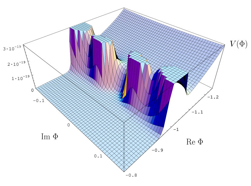
Figure 4: Effective potential in the theory $W=\zeta(\phi+2-\sqrt{3})+C_{1}(\phi+C_{2})(1-\tanh(C_{3}(\phi+C_{2})))$ as a function of $\mathop{\rm Re}\nolimits\phi$ and $\mathop{\rm Im}\nolimits\phi$.

The main goal of presenting these models was to demonstrate that with a proper choice of the superpotential one can obtain a broad variety of potentials, even in the theories with a single chiral multiplet with a minimal Kähler potential. In particular, one can have models with such potentials where in the early universe one has efficient gravitino production, whereas at the end of the process one has $m_{3/2}\sim 10^{2}$ GeV, and a nearly vanishing vacuum energy density $V\sim 10^{-29}$ g cm^-3, consistent with the observational data.

Before one becomes too excited, one should remember that near the minimum of the effective potential all these models look like the simple Polónyi model with $W=\zeta(\phi+2-\sqrt{3})$. This is good, because the vacuum energy in the minimum of the effective potential in this model vanishes, but $m_{3/2}$ does not, so we definitely have production of gravitinos with helicity ${\textstyle\frac{1}{2}}$ in this model. However, it is also bad, because the gravitino production in the Polónyi model only exacerbates the moduli problem [61] which exists in this theory. The energy density stored in the oscillating Polónyi field $\phi$ typically leads to a much greater conflict with the observational data than the decay of gravitinos produced during the oscillations of the field $\phi$. Note, however, that the physical origin of the gravitino problem differs from that of the moduli problem, so, in general, the problem of gravitinos produced after inflation may appear even in the models where the moduli problem can be solved.

10.3 Theories with two chiral multiplets

To examine more realistic models of gravitino production, one should consider theories with more than one chiral multiplet. Here the situation becomes even more complicated. It was extremely difficult to derive equations for the gravitino in such models. Solving them presents an even greater challenge and requires more effort. In this paper we will only give several comments on this subject.

First of all, one may try, whenever possible, to reduce the problem involving two chiral multiplets to the theory of one multiplet. We have shown in section 9.5 that this can be done in some cases when one of the scalar fields has a much greater energy density than all the other fields.

However, in other cases this method may not work. For example, the simplest supersymmetric version of the hybrid inflation scenario studied in [33] has a very interesting property. After the end of inflation, two scalar fields fall down to the minimum of the effective potential simultaneously and oscillate synchronously, as a single field. For this reason it was assumed in [33] that one can use (9.3) to study the gravitino production, just as in the theory with one chiral multiplet. However, according to [33], $\Delta^{2}=1-|\hat{A}|^{2}$ can be ${\rm O}(1)$ in this model. However, in this case the second equation in the system of equations (9.20) derived in our paper implies that $\Upsilon\not=0$. Therefore, instead of solving (9.3) one should solve the system of two equations (9.20). This is a much more complicated problem; it was not addressed in [33].

Even more importantly, the existence of gravitino production in the very early universe is not a guarantee of their survival until the late stages of the evolution of the universe. This issue requires a special investigation, and the answer may be model-dependent.

Indeed, suppose for a moment that the gravitino–goldstino correspondence is valid at all stages of the process, and instead of solving equations for the gravitino in supergravity one can solve equations for the chiral fermions $\chi_{i}$ in the underlying globally supersymmetric theory. Then one may wonder whether the particles produced after inflation are gravitinos, or usual chiral fermions, superpartners of the inflaton, which can be called an inflatino [36].

As we have already mentioned, supersymmetry is always broken during the expansion of the universe supported by the energy density of scalar fields. Suppose, however, that the relatively small supersymmetry breaking remaining when the universe slows down involves chiral fermions belonging to the hidden sector, such as the Polónyi field. Suppose also that the inflaton field $\phi_{1}$ does not interact with the Polónyi field $\phi_{2}$ in the limit $M_{P}\to\infty$. As an example of such a theory one may consider the theory with the superpotential $W=m_{\phi}\phi_{1}^{2}/2+\zeta(\phi_{2}+2-\sqrt{3})$ or $W=\sqrt{\lambda}\phi_{1}^{3}/3+\zeta(\phi_{2}+2-\sqrt{3})$.

Soon after inflation, the energy density is dominated by the energy of the inflaton field, i.e.  $\rho\approx\rho_{1}$ is many orders of magnitude greater than $\rho_{2}$. In the expression for the effective potential of the Polónyi field there is a term $\exp(\phi_{2}^{2}/M_{P}^{2})|W_{1}|^{2}$. This term at $\phi_{2}\ll M_{p}$ becomes $(1+{\phi_{2}^{2}/M_{P}^{2}})\rho_{1}\approx(\rho_{1}+3\phi_{2}^{2}H^{2})$, which implies that the effective potential for the Polónyi field in the early universe has a minimum at $\phi_{2}\approx 0$, and the mass squared of this field is $m_{2}^{2}\approx 3H^{2}$. (Note that in order to go to the canonically normalized field one should divide $\phi_{2}$ by $\sqrt{2}$.) Therefore, the field $\phi_{2}$ rapidly oscillates about $\phi_{2}=0$. The amplitude of oscillations decreases as $a^{-1}$, which eventually puts this field at the vicinity of the point $\phi_{2}=0$, where it stays until $H$ drops below ${\rm O}(m_{3/2})$. At that stage the Polónyi field starts rolling towards the flat-space minimum of its potential at $\phi_{2}=M_{P}(\sqrt{3}-1)$, and oscillates about it. The energy density of this field decreases very slowly, which constitutes the essence of the moduli problem as formulated in [62]. We will not consider this problem here, but one should remember that in a realistic cosmological model based on supergravity this problem should be taken into account and resolved.

The solution for the goldstino in this model in the limit $M_{P}\to\infty$ is given by (9.38), so that at the early stages, when $\rho_{1}$ dominates, one has $\upsilon=\rho_{1}^{1/2}{\rm e}^{\gamma_{0}\int{\rm d}t\,\mu_{1}}(\chi_{1}+\chi^{1})$. Therefore, one can use the results of our previous investigation of the gravitino production [22, 27, 30] to estimate the number of gravitinos produced at that stage.

However, eventually the energy density of the oscillating field $\phi_{1}$ drops down, and the energy becomes dominated by the energy density of the oscillating Polónyi field. At that stage one has $\upsilon=\rho_{2}^{1/2}{\rm e}^{\gamma_{0}\int{\rm d}t\,\mu_{2}}(\chi_{2}+\chi^{2})$ (except for at that stage one should use a more accurate expression because the effective potential of the Polónyi field cannot be correctly described in the limit $M_{P}\to\infty$).

Thus one may argue that the efficient production of the chiral fermions $\chi_{1}$, which can be interpreted as the process of gravitino production at the first stage of the process, does not imply anything about the density of gravitinos at the second stage: the gravitino must first spit the chiral fermion $\chi_{1}$, and then eat the chiral fermion $\chi_{2}$, if there are any of them around. However, in this model one does not expect efficient production of the fermions $\chi_{2}$ at the stage of the oscillations of the Polónyi field, so at the end of the process one will have many fermions $\chi_{1}$ (inflatino) and practically no gravitinos with helicity ${\textstyle\frac{1}{2}}$.

This argument is very interesting but insufficient to give a definite answer to the question concerning the number of gravitinos at the last stages of the process. It is based on the assumption that the fermions $\chi_{i}$ do not mix with each other, so that the fermions $\chi_{1}$ produced at the first stage of the process cannot be converted into $\chi_{2}$. This assumption is justified in the limit $M_{P}\to\infty$, but in this limit there is no expansion of the universe, the ratio $\rho_{2}/\rho_{1}$ is constant and the definition of the goldstino does not change in time. The transition from the regime $\rho_{1}\gg\rho_{2}$ to the regime $\rho_{2}\gg\rho_{1}$ in the expanding universe takes time ${\rm O}(H^{-1})\sim M_{p}/\sqrt{\rho}$. This time interval becomes infinitely long in the limit $M_{p}\to\infty$.

Thus one may wonder whether some of the particles $\chi_{1}$ can convert to $\chi_{2}$ at the intermediate stage of the process, when $\rho_{1}\sim\rho_{2}$ and the definition of the goldstino gradually changes from $\rho_{1}^{1/2}{\rm e}^{\gamma_{0}\int{\rm d}t\,\mu_{1}}(\chi_{1}+\chi^{1})$ to $\rho_{2}^{1/2}{\rm e}^{\gamma_{0}\int{\rm d}t\,\mu_{2}}(\chi_{2}+\chi^{2})$. In order to study this question one should go beyond the approximation $M_{P}\to\infty$, i.e. one cannot apply the gravitino–goldstino equivalence theorem used in the argument given above.

One may try to approach this issue in a more direct and unambiguous way, using the system of equations (9.20) for $\theta$ and $\Upsilon$ in the unitary gauge. This is a much more powerful method. As we have emphasized, this method applies at all stages of the process, because the only condition required for its validity, $H^{2}+m^{2}_{3/2}>0$, is always satisfied in the FRW universe. It allows one to avoid using imprecise language based on the gravitino–goldstino equivalence and the limit $M_{P}\to\infty$. Also, it allows us to formulate adequate initial conditions for the gravitino equations at the end of inflation (see section 10.1).

In this formalism one could expect that the total number of massive gravitinos with helicity ${\textstyle\frac{1}{2}}$ can be represented by some adiabatic invariant, so the gravitinos produced at the first stage of the process cannot simply disappear because of the change of the regime if this change is slow enough (adiabatic). Moreover, one could even expect that if this change is not adiabatic, it may lead to an additional gravitino production similar to that discussed in [32]. Consider, for example, the model with $W=m_{\phi}\phi_{1}^{2}/2+\zeta(\phi_{2}+2-\sqrt{3})$ with $m_{\phi}\sim 10^{13}$ GeV, as in the previous section. In this model, at the first stage of the process one has $\mu_{1}\sim m_{\phi}\sim 10^{13}$ GeV. Then, within the time $H^{-1}\sim{m^{-1}_{3/2}}$ this parameter drops down to ${\rm O}(m_{3/2})\sim 10^{2}$ GeV. The last stages of this process are non-adiabatic. An estimate similar to that made in the previous section indicates the possibility of production of gravitinos with $n_{3/2}\sim 10^{-2}(m_{\phi}m_{3/2})^{3/2}$. If one ignores for a moment the moduli problem and assumes that the energy of the scalar field $\phi_{2}$ immediately transfers to thermal energy as soon as it begins oscillating, one finds $s\sim(M_{P}m_{3/2})^{3/2}$ and ${n_{3/2}\over s}\sim 10^{-2}\left({m_{\phi}\over M_{P}}\right)^{3/2}$, as in (10.6).

However, the situation is, in fact, more complicated, and the arguments based on adiabaticity must be examined in a detailed way. They should be applicable at the time before and after the change of the regime from $\rho_{1}\gg\rho_{2}$ to $\rho_{1}\ll\rho_{2}$, but they may not apply at the transitional stage when the energy densities of the scalar fields $\phi_{1}$ and $\phi_{2}$ become comparable. At that time the fields $\theta$ and $\Upsilon$ start mixing because of the term $\vec{k}^{2}\Delta^{2}\theta$ in (9.44), so at that intermediate epoch the number of gravitinos, generally speaking, is not conserved. This resembles the neutrino oscillations, when the neutrino registered in the detector may be different from the neutrino emitted by the Sun. Without performing a quantization of the system of coupled fields $\theta$ and $\Upsilon$ and solving the corresponding equations in the time-dependent background, one cannot tell whether the number of gravitinos becomes depleted at the transitional stage, or, vice versa, the existence of this stage creates a new type of non-adiabaticity which may enhance gravitino production.

We hope that the results of our investigation create a proper framework which may help to address these questions.

10.4 Other mechanisms of gravitino production

There exist some other mechanisms of gravitino production, which we did not discuss in this paper, and which can be particularly interesting in the context of hybrid inflation. We will briefly describe them here.

These mechanisms are related to the possibility that the scalar fields are inhomogeneous, or that other oscillating fields, such as vector fields, appear in the universe. We did not consider this possibility in the main part of our paper because all fields become nearly homogeneous during inflation, and vector fields become extremely small. However, in some models inhomogeneous scalar fields and vector fields may rapidly appear soon after the end of inflation.

The first mechanism is related to the formation of cosmic strings, which is a typical property of the hybrid inflation scenario [56, 57]. These cosmic strings, associated with the topologically stable configuration of the complex scalar fields $z_{i}$, interact with the gravitino field $\psi_{\mu}$. Dynamics of the strings lead to emission of gravitinos. Indeed, the generic gravitino master equation (6.21) is constructed with the long covariant derivative ${\cal D}_{\mu}\psi_{\nu}=\left(\partial_{\mu}+{\textstyle\frac{1}{4}}\omega_{\mu}^{ab}(e)\gamma_{ab}+{\textstyle\frac{1}{2}}{\rm i}A_{\mu}^{B}\gamma_{5}\right)\psi_{\nu}-\Gamma_{\mu\nu}^{\lambda}\psi_{\lambda}$, which contains, in particular, a bosonic part of the $U(1)$ connection, $A_{\mu}^{B}$. In the gauge that is not singular at $W=0$, the form of $A_{\mu}^{B}$ is given by equation (5.26), $A_{\mu}^{B}={\textstyle\frac{1}{2}}{\rm i}\left[(\partial_{i}{\cal K}){\partial}_{\mu}z^{i}-(\partial^{i}{\cal K}){\partial}_{\mu}z_{i}\right]+M_{P}^{-2}W_{\mu}^{\alpha}{\cal P}_{\alpha}$. Consider for simplicity the minimal Kähler potential ${\cal K}=z_{i}z^{i}$. Then in the long covariant derivative we will have a term $J_{\mu}=z_{i}{\partial}_{\mu}z^{i}-z^{i}{\partial}_{\mu}z_{i}$, which does not vanish for the complex field configuration around the string. Spacetime variations of the term $J_{\mu}(t,{\vec{x}})$ due to the motion and excitations of the string will lead to the radiation of gravitinos by the string, similar to the gravitational radiation from the cosmic strings.

However, the term $J_{\mu}(t,{\vec{x}})$ may appear in the gravitino equations even in the cases where strings are not generated. For example, very strong spinodal (tachyonic) instability of scalar field fluctuations at the ‘waterfall’ stage in the hybrid inflation results in a very rapid decay of the homogeneous inflaton field into inhomogeneous classical scalar fields in the model. For the inhomogeneous complex scalar fields we also have a non-vanishing term $J_{\mu}(t,{\vec{x}})$, which leads to additional gravitino production.

In both cases the magnitude of $J_{\mu}(t,{\vec{x}})$ is proportional to the small quantity $|\phi|^{2}M_{P}^{-4}$, where $|\phi|$ is the typical amplitude of the scalar field. Therefore, the gravitino production in this case can be studied using perturbation theory. The net gravitino abundance will depend on the duration of the gravitino emission. One may think about gravitino production in this case as resulting from collisions of classical waves of various scalar fields. One may also consider gravitino production due to the collisions of non-thermalized particles produced at the first stages of preheating. This and other mechanisms of gravitino production after inflation deserve a separate investigation.

11 Discussion

The initial goal of our investigation was rather limited. We wanted to study the gravitino production by an oscillating scalar field at the end of inflation. However, soon we discovered that the existing tools that we could use in our work were not quite adequate.

We have found that it is rather difficult to study the conformal properties of gravitinos in the standard formulation of supergravity. This forced us to reformulate phenomenological supergravity in a way revealing its hidden superconformal symmetry $SU(2,2|1)$. Until now, the superconformal version of phenomenological supergravity was only used as a tool for the derivation of phenomenological supergravity, We have found that this formulation has several important advantages over the standard one.

The superconformal formulation of supergravity may simplify the investigation of the processes in the early universe. Indeed, the FRW universe is conformally flat. Therefore, by making appropriate redefinitions of the fields and the metric in a conformally invariant theory, one can reduce the investigation of all processes in an expanding FRW universe to an investigation of processes in Minkowski space. We did not use this method in our work, but it may be extremely interesting and rewarding to study the standard issues of big-bang cosmology from this new perspective.

For us it was important that the $SU(2,2|1)$ formulation of supergravity provides a flexible framework unifying various formulations of $N=1$ supergravity interacting with matter, depending on the choice of the $R$-symmetry fixing. It explains the superconformal origin of the Fayet–Iliopoulos terms. It also allows us to study the weak-coupling limit of supergravity, $M_{P}\rightarrow\infty$, and to formulate the gravitino–goldstino equivalence theorem which is valid in this limit. Indeed, it is not very simple to make sense out of this limit in the standard versions of $N=1$ supergravity unless one makes a certain field rescaling, which brings us back to the original field variables of the underlying superconformal theory. This made it possible to prove the equivalence theorem, which explains why gravitino production in the early universe in some models is not suppressed in the limit of weak gravitational coupling, $M_{P}\to\infty$.

The superconformal formulation helped us to study the super-Higgs effect in cosmology and to derive the equations for the gravitino interacting with any number of chiral and vector multiplets in the gravitational background with varying scalar fields.

There are several other aspects related to the superconformal formulation which require further study. One of them is the possible existence of strings associated with the lines where the conformon field vanishes. Such objects could not appear in the usual $N=1$ supergravity where $M_{P}$ is already fixed. Note that the conformon field does not have any dynamical degrees of freedom associated with it; it can be set equal to $M_{P}$ everywhere where it does not vanish. However, this does not include the string, where this field vanishes and the vector field $A_{\mu}$ exists. It would be very interesting to study the question of whether the strings which may appear in the $SU(2,2|1)$ formulation of supergravity may have any interesting dynamics associated with them. In such a case one would have stringy excitations as part of supergravity.

Returning to the problem of gravitino production, we should note that the derivation of the gravitino equations was only part of the problem; it is very difficult to find their solutions in the cosmological background. We analysed them in some particular cases and studied their properties, which can be helpful for a future investigation of gravitino production in realistic models based on supergravity. The main conclusion is that due to the gravitino–goldstino equivalence theorem, the production of gravitinos in the very early universe can be as efficient as the production of ordinary spin-${\textstyle\frac{1}{2}}$ fermions, i.e. it is suppressed by small coupling constants such as $\lambda$ or $g^{2}$, but not by the gravitational coupling.

Thus, despite naive expectations, gravitinos created by the oscillating scalar fields soon after inflation may provide a contribution to the matter content of the universe as large as that from the usual particles. This result can be quite important for our understanding of the physical processes in the very early universe.

On the other hand, the definition of the gravitino (and goldstino) in the early universe changes in time. Therefore, an additional investigation is required to check whether the number of gravitinos produced soon after the end of inflation is conserved until the late stages of the evolution of the universe, or they become converted to other, less harmful, particles. The answer to this question may be model dependent. Many models based on supergravity are plagued by the moduli problem, which is usually even more severe than the problem of the gravitino created after inflation. During the last few years there have been many attempts to solve the moduli problem. One of the possible solutions involves an additional short stage of the late-time ‘thermal’ inflation [63]. If this mechanism solves the moduli problem, it may solve the gravitino problem as well.

However, in some models the gravitino problem may be as severe or even more severe than the moduli problem. For example, in the supersymmetric versions of the hybrid inflation scenario all coupling constants are ${\rm O}(10^{-1})$. A full investigation of gravitino production in such models have not been performed as yet, but preliminary estimates indicate that the ratio $n_{3/2}/n_{s}$ at the first stages of preheating can be as large as ${\rm O}(1)$ [22, 27, 30]. This may lead to drastic cosmological consequences, unless the gravitinos created soon after inflation become converted into less harmful particles at the stage when the energy density of the inflaton field becomes sub-dominant and the definition of the gravitino changes. Therefore, it is very important to study whether the gravitino conversion is actually possible. We hope that this problem, as well as other issues related to the physical properties of the gravitinos in the early universe, can be addressed using the formalism developed in our paper.

Acknowledgments

It is a pleasure to thank P. Binétruy, A. Chamseddine, G.F. Giudice, P. Greene, H.P. Nilles, A. Riotto, I. Tkachev, W. Troost and S. Vandoren for useful discussions. The work of R.K and A.L. was supported by NSF grant PHY-9870115, L.K. was supported by NSERC and CIAR. A.V.P. thanks the Department of Physics at Stanford and the CERN theory division for the hospitality. L.K. and A.L. thank NATO Linkage Grant 975389 for support.

Appendix A Notation

We mostly use the notation of [5], which agrees with [6]. However, rather than using the index range $\mu=1,2,3,4$, for curved indices we use $\mu=1,2,3,0$, thus converting the metric $(++++)$ in [5] into the familiar $(+++-)$. In the same token, the Levi–Civita tensor $\varepsilon^{abcd}$ (with flat indices $a=1,2,3,4$) is taken to be imaginary. Indeed, we have $\varepsilon^{0123}={\rm i}$. The normalization for $\gamma_{5}=\varepsilon^{0123}\gamma_{0}\gamma_{1}\gamma_{2}\gamma_{3}$ is chosen such that ${\textstyle\frac{1}{2}}\varepsilon^{abcd}\gamma_{cd}=-\gamma_{5}\gamma^{ab}$. The comparison with [5] is $\gamma_{4}=-{\rm i}\gamma_{0}$. Then $\gamma_{0}$ is anti-Hermitian, while $\vec{\gamma}$ (where this denotes the spacelike components) and $\gamma_{5}$ are Hermitian. Furthermore, for antisymmetrization, we use $[ab]=\frac{1}{2}(ab-ba)$. An explicit realization of $\gamma$-matrices is

$$\gamma_{0}=\pmatrix{{\rm i}{\mathchoice{\mathrm{1\mskip-4.0mul}}{\mathrm{1\mskip-4.0mul}}{\mathrm{1\mskip-4.5mul}}{\mathrm{1\mskip-5.0mul}}}_{2}&0\cr 0&-{\rm i}{\mathchoice{\mathrm{1\mskip-4.0mul}}{\mathrm{1\mskip-4.0mul}}{\mathrm{1\mskip-4.5mul}}{\mathrm{1\mskip-5.0mul}}}_{2}\cr}\ ;\qquad\vec{\gamma}=\pmatrix{0&-{\rm i}\vec{\sigma}\cr{\rm i}\vec{\sigma}&0\cr}\ ;\qquad\gamma_{5}=\pmatrix{0&-{\mathchoice{\mathrm{1\mskip-4.0mul}}{\mathrm{1\mskip-4.0mul}}{\mathrm{1\mskip-4.5mul}}{\mathrm{1\mskip-5.0mul}}}_{2}\cr-{\mathchoice{\mathrm{1\mskip-4.0mul}}{\mathrm{1\mskip-4.0mul}}{\mathrm{1\mskip-4.5mul}}{\mathrm{1\mskip-5.0mul}}}_{2}&0\cr}\,.$$ (A.1)

We use also left and right projections

$$P_{L}={\textstyle\frac{1}{2}}(1+\gamma_{5})\,,\qquad P_{R}={\textstyle\frac{1}{2}}(1-\gamma_{5})\,.$$ (A.2)

The Majorana condition, defined by $-{\rm i}\lambda^{\dagger}\gamma_{0}=\lambda^{T}{\cal C}$, with ${\cal C}$ the charge conjugation $\gamma_{0}\gamma_{2}$ in this representation, then amounts to

$$\lambda^{*}=\pmatrix{0&-\sigma_{2}\cr\sigma_{2}&0}\lambda\,.$$ (A.3)

The barred spinors are Majorana conjugates. For the chiral spinors, e.g. $\lambda_{L}\equiv P_{L}\lambda$, not being Majorana spinors, this implies

$$\bar{\lambda}_{L}\equiv(\lambda_{L})^{T}{\cal C}=\bar{\lambda}P_{L}=-{\rm i}(\lambda_{R})^{\dagger}\gamma_{0}\,.$$ (A.4)

For more detailed explanations, see, e.g., [50].

The Einstein tensor and energy–momentum tensor are

$$R_{\mu\nu}{}^{ab} = 2\partial_{[\mu}\omega_{\nu]}{}^{ab}+2\omega_{[\mu}{}^{ac}\omega_{\nu]c}{}^{b}$$

$$R_{\mu\nu} = R_{\mu\rho}{}^{ab}e^{\rho}_{a}e_{\nu}^{b}\,,\qquad R=g^{\mu\nu}R_{\mu\nu}$$

$$G_{\mu\nu} = e^{-1}\frac{\delta}{\delta g^{\mu\nu}}\int{\rm d}^{4}x\,eR=R_{\mu\nu}-{\textstyle\frac{1}{2}}g_{\mu\nu}R$$

$$T_{\mu\nu} = -e^{-1}e_{\nu}^{a}\frac{\delta}{\delta e^{\mu}_{a}}M_{P}^{-2}\int{\rm d}^{4}x\,{\cal L}^{(m)}\,,$$ (A.5)

with ${\cal L}^{(m)}$ the matter action, i.e. all but the graviton term. Due to invariance under Lorentz rotations, $T_{\mu\nu}$ is symmetric by use of field equations.

Complex conjugation by definition reverses the order of the spinors. The action of complex conjugation on spinors is often complicated. A simpler equivalent procedure is taking the charge conjugate. For pure bosonic numbers this is just complex conjugation. For matrices in spinor space, we have $\gamma_{\mu}^{C}=\gamma_{\mu}$ and $\gamma_{5}^{C}=-\gamma_{5}$. For this operation we do not have to interchange the spinors. Majorana spinors are invariant under this operation, but the chiral spinors change chirality. The same holds for the barred (Majorana conjugate) spinors. In our notation for chiral multiplets, the operation thus interchanges upper with lower $i$ indices, but does not change gauge indices $\alpha$. As a practical summary of the rules, see the following equations:

$$X_{I}^{C}=X^{I}\,,\qquad Y^{C}=Y^{*}\,,\qquad z_{i}^{C}=z^{i}\,,\qquad\phi_{i}^{C}=\phi^{i}\,,$$

$$\gamma_{\mu}^{C}=\gamma_{\mu}\,,\qquad\gamma_{5}^{C}=-\gamma_{5}\,,\qquad P_{L}^{C}=P_{R}$$

$$\Omega_{I}^{C}=\Omega^{I}\,,\qquad\chi_{i}^{C}=\chi^{i}\,,\qquad\bar{\chi}_{i}^{C}=\bar{\chi}^{i}\,,$$

$$\lambda^{\alpha\,C}=\lambda^{\alpha}\,,\qquad\lambda^{\alpha}_{L}{}^{C}=\lambda^{\alpha}_{R}\,,\qquad{\cal P}_{\alpha}{}^{C}={\cal P}_{\alpha}\,.$$ (A.6)

An example of these rules can be seen by obtaining the second line from the first line in (7.11), where at the end one also checks the charge conjugation invariance of $\delta\lambda^{\alpha}$ due to the charge conjugation invariance of ${\rm i}\gamma_{5}$. For more intrinsic definitions of the charge conjugation operation, see [50].

Appendix B Conformal metric

We take a conformal metric, i.e.

$$e^{a}_{\mu}=a(\eta)\delta_{\mu}^{a}\,,\qquad g_{\mu\nu}=a^{2}(\eta)\eta_{\mu\nu}\,,$$ (B.1)

where $\eta=x^{0}$ is a time coordinate. However, to start with, we will still allow $a$ to be a general scalar function of spacetime. The connections are then (from now on, indices are raised and lowered with flat metric $\eta_{\mu\nu}$)

$$\omega^{ab}_{\mu}=2\delta_{\mu}^{[a}\partial^{b]}\ln a\,,\qquad\Gamma^{\rho}_{\mu\nu}=2\delta_{(\nu}^{\rho}\partial_{\mu)}\ln a-\eta_{\mu\nu}\partial^{\rho}\ln a\,.$$ (B.2)

The curvature is then

$$R^{\mu}{}_{\nu\rho\sigma} = \eta_{\nu\nu^{\prime}}\left[4\delta^{[\mu}_{[\sigma}\partial_{\rho]}\partial^{\nu^{\prime}]}\ln a+4\delta_{[\rho}^{[\mu}(\partial^{\nu^{\prime}]}\ln a)(\partial_{\sigma]}\ln a)-2\delta_{[\rho}^{[\mu}\delta_{\sigma]}^{\nu^{\prime}]}(\partial\ln a)^{2}\right]$$

$$R_{\mu\nu} = 2\partial_{\mu}\partial_{\nu}\ln a-2(\partial_{\mu}\ln a)(\partial_{\nu}\ln a)+\eta_{\mu\nu}[{\,\lower 0.9pt\vbox{\hrule\hbox{\vrule height=5.69046pt\hskip 5.69046pt\vrule height=5.69046pt}\hrule}\,}\ln a+2(\partial\ln a)^{2}]$$

$$a^{2}R = 6{\,\lower 0.9pt\vbox{\hrule\hbox{\vrule height=5.69046pt\hskip 5.69046pt\vrule height=5.69046pt}\hrule}\,}\ln a+6(\partial\ln a)^{2}$$

$$G_{\mu\nu} = 2\partial_{\mu}\partial_{\nu}\ln a-2(\partial_{\mu}\ln a)(\partial_{\nu}\ln a)-\eta_{\mu\nu}[2{\,\lower 0.9pt\vbox{\hrule\hbox{\vrule height=5.69046pt\hskip 5.69046pt\vrule height=5.69046pt}\hrule}\,}\ln a+(\partial\ln a)^{2}]\,.$$ (B.3)

The Lorentz connection term in covariant derivatives on spinors is

$$+{\textstyle\frac{1}{4}}\omega^{ab}_{\mu}\gamma_{ab}=+{\textstyle\frac{1}{2}}\delta_{\mu}^{a}\gamma_{a}{}^{b}\delta_{b}^{\nu}\partial_{\nu}\ln a\,.$$ (B.4)

Using these expressions we obtain useful equations for the covariant derivatives of the gravitino (in this appendix the Kähler connections are omitted), for example,

$$a\not\!\!{\cal D}\psi_{\mu}\equiv\overline{\not\!\partial}\psi_{\mu}+{\textstyle\frac{1}{2}}\left(\overline{\not\!\partial}\ln a\right)\psi_{\mu}+\overline{\gamma}_{\mu}(\partial_{\sigma}\ln a)\eta^{\nu\sigma}\psi_{\nu}-\overline{\gamma}\cdot\psi\partial_{\mu}\ln a\,.$$ (B.5)

Now we specify the case that $a$ depends only on the time coordinate, which is called $\eta$. It is, however, easy to express derivatives with respect to a time coordinate defined by ${\rm d}t=a(\eta)\,{\rm d}\eta$. We thus introduce

$$\dot{a}\equiv\frac{\partial_{0}a}{a}\,,$$ (B.6)

and also the Hubble parameter

$$H=\frac{\dot{a}}{a}=\frac{\partial_{0}a}{a^{2}}\,.$$ (B.7)

Then we have the following expressions for covariant derivatives where we use the notation introduced at the beginning of section 7,

$${\cal D}_{\mu}\chi = \partial_{\mu}\chi-{\textstyle\frac{1}{2}}\overline{\gamma}_{\mu 0}\dot{a}\chi$$

$$a\not\!\!{\cal D}\chi = \overline{\not\!\partial}\chi+{\textstyle\frac{3}{2}}\gamma^{0}\dot{a}\chi$$

$${\cal D}_{\mu}\psi^{\mu} = \partial^{\mu}\psi_{\mu}-2a^{-2}\dot{a}\psi_{0}+{\textstyle\frac{1}{2}}a^{-2}\dot{a}\gamma_{0}\vec{\gamma}\cdot\vec{\psi}$$

$$a\not\!\!{\cal D}\psi_{\mu} = \overline{\not\!\partial}\tilde{\psi}_{\mu}-\dot{a}\left(\overline{\gamma}_{\mu}\psi_{0}+{\textstyle\frac{1}{2}}\gamma_{0}\psi_{\mu}+\overline{\gamma}\cdot\psi\delta_{\mu}^{0}\right)\,.$$ (B.8)

Furthermore, we now have

$$-M^{-2}_{P}\rho\equiv G^{0}{}_{0} = -3a^{-2}(\partial_{0}\ln a)^{2}=-3H^{2}$$

$$-M^{-2}_{P}p{\mathchoice{\mathrm{1\mskip-4.0mul}}{\mathrm{1\mskip-4.0mul}}{\mathrm{1\mskip-4.5mul}}{\mathrm{1\mskip-5.0mul}}}_{3}\equiv G =a^{-2} {\mathchoice{\mathrm{1\mskip-4.0mul}}{\mathrm{1\mskip-4.0mul}}{\mathrm{1\mskip-4.5mul}}{\mathrm{1\mskip-5.0mul}}}_{3}\left[2\partial_{0}^{2}\ln a+(\partial_{0}\ln a)^{2}\right]={\mathchoice{\mathrm{1\mskip-4.0mul}}{\mathrm{1\mskip-4.0mul}}{\mathrm{1\mskip-4.5mul}}{\mathrm{1\mskip-5.0mul}}}_{3}(3H^{2}+2\dot{H})\,,$$ (B.9)

where $G$ denotes the $3\times 3$ part of $G^{\mu}{}_{\nu}$ in the spacelike directions.

The condition for a de Sitter metric is $p=-\rho$ which implies that $H$ is constant. We then have

$$a^{-1} = H(C-\eta)$$

$$R_{\mu\nu}{}^{\rho\sigma} = 2\delta_{\mu}^{[\rho}\delta_{\nu}^{\sigma]}H^{2}$$

$$R = -12H^{2}=-4VM_{P}^{-2}$$

$$G_{\mu\nu} = -{\textstyle\frac{1}{4}}g_{\mu\nu}R=g_{\mu\nu}VM_{P}^{-2}\,,$$ (B.10)

where $C$ is also a constant, and we also gave the expression in terms of the constant value of the potential $V$.

Appendix C Kähler geometry from the conformal formulation

In this section we make the transition from the scalar action in terms of ${\cal N}_{I}{}^{J}$ to a Kählerian action. The proof that we present here can also be applied to the $N=2$ theory as to $N=1$.

Theorem.

We consider the action

$${\cal L}=-{\cal N}_{I}{}^{J}{\cal D}_{\mu}X^{I}{\cal D}^{\mu}X_{J}$$ (C.1)

in terms of $n+1$ complex scalars $X^{I}$ (where $X_{I}$ are their complex conjugates). In (C.1) the covariant derivatives have a $U(1)$ connection, and we write them as

$${\cal D}_{\mu}X_{I}=\partial_{\mu}X_{I}+{\textstyle\frac{1}{3}}{\rm i}A_{\mu}X_{I}\,,\qquad{\cal D}_{\mu}X^{I}=\partial_{\mu}X^{I}-{\textstyle\frac{1}{3}}{\rm i}A_{\mu}X^{I}\,.$$ (C.2)

The functions ${\cal N}_{I}{}^{J}$ depend on $X^{I}$ and $X_{I}$, and satisfy

$$X^{I}\frac{\partial}{\partial X^{K}}{\cal N}_{I}{}^{J}=X^{K}\frac{\partial}{\partial X^{K}}{\cal N}_{I}{}^{J}=0\,,$$ (C.3)

and their complex conjugates. Note that here we took ${\cal N}_{I}{}^{J}$ as the basic object, rather than as the second derivative of a scalar ${\cal N}$. If it is the second derivative, as in the main text, then the two equations are equivalent.

One can choose $n$ complex coordinates $z_{i}$ (and complex conjugates $z^{i}$) by defining

$$X_{I}=Yx_{I}(z)\,,\qquad X^{I}=Y^{*}x^{I}(z^{*})\,,$$ (C.4)

where $x_{I}(z)$ are $n+1$ non-degenerate arbitrary holomorphic functions of the $z_{i}$, and $Y$ is the $(n+1)$th complex variable. The action can then be written as

$${\cal L} = -\frac{1}{4}{\cal N}^{-1}\left(\partial_{\mu}{\cal N}\right)^{2}-\frac{1}{9}{\cal N}\left(A_{\mu}+\frac{{\rm i}}{2}\left(\partial^{i}{\cal K}\,\partial_{\mu}z_{i}-\partial_{i}{\cal K}\,\partial_{\mu}z^{i}\right)-\frac{3{\rm i}}{2}\partial_{\mu}\ln\frac{Y}{Y^{*}}\right)^{2}$$ (C.5)

$$+\frac{1}{3}{\cal N}\left(\partial^{j}\partial_{i}{\cal K}\right)\partial_{\mu}z^{i}\,\partial^{\mu}z_{j}\,,$$

where

$${\cal N} \equiv X^{I}{\cal N}_{I}{}^{J}X_{J}$$

$${\cal K}(z,z^{*}) \equiv -3\ln\left[-{\textstyle\frac{1}{3}}x^{I}(z^{*}){\cal N}_{I}{}^{J}(z,z^{*})x_{J}(z)\right]\,.$$ (C.6)

This scalar function ${\cal N}$ coincides with the one that we started with in the main text.

Interpretation.

The metric defines a cone (using $r^{2}=-{\cal N}$ one obtains the canonical parametrization ${\rm d}s^{2}={\rm d}r^{2}+r^{2}\ldots$). When $U(1)$ is not gauged ($A_{\mu}=0$), the base of the cone (the manifold with fixed ${\cal N}$) is a Sasakian manifold with a $U(1)$ invariance. Here we gauge $U(1)$, which implies that the auxiliary field $A_{\mu}$ can be redefined such that the second term of the first line of (C.5) is pure auxiliary and can also be deleted. Then one is left with a Kähler manifold with the Kähler potential ${\cal K}$. We are interested in the Kählerian action for $n$ independent complex scalars $z_{i}$ on the submanifold of the $(n+1)$-complex-dimensional manifold defined by a constant value of ${\cal N}$. This is a real condition, but the $U(1)$ invariance implies that another real variable disappears.

Application.

In practice, the fields may have a further gauge-connection. In that case the $\partial_{\mu}$ which we write here, can be replaced by a suitably covariant derivative.

In $N=1$, the matrix ${\cal N}_{I}{}^{J}$ emerges from the superconformal tensor calculus as the second derivative of a scalar function ${\cal N}$, and (C.3) is the last equation of (3.5). In $N=2$ this treatment is appropriate in all cases where a prepotential $F(X)$ exists. The matrix ${\cal N}_{I}{}^{J}$ is the imaginary part of the second derivative of the holomorphic prepotential, whose third derivative satisfies $X^{K}F_{IJK}=0$ [16]. Note that the notation which we adapt here is not the usual one for that case, but identifying further ${\cal N}_{I}{}^{J}$ with $-2{\rm i}(F_{IJ}-F^{*}_{IJ})$, our formulation is also applicable to $N=2$ as to $N=1$.

We will adopt the dilatational gauge-fixing condition

$${\cal N}=-3M_{P}^{2}\,.$$ (C.7)

Its normalization is chosen appropriately for $N=1$. For $N=2$ the normalization changes due to contributions of a second compensating multiplet to the $eR$ term in the action [55].

Construction.

We first combine the terms which include the auxiliary field $A_{\mu}$. Writing the action (C.1) as ${\cal L}(A_{\mu})$, we have

$${\cal L}(A_{\mu}) = -{\textstyle\frac{1}{9}}{\cal N}(A_{\mu}-\tilde{A}_{\mu})^{2}+{\cal L}(\tilde{A}_{\mu})$$

$$\tilde{A}_{\mu} \equiv \frac{3{\rm i}}{2{\cal N}}\left[X^{I}{\cal N}_{I}{}^{J}(\partial_{\mu}X_{J})-(\partial_{\mu}X^{I}){\cal N}_{I}{}^{J}X_{J}\right]\,.$$ (C.8)

With the coordinates as in (C.4), the last part of (C.3) implies that ${\cal N}_{I}{}^{J}$ depends only on $z^{i}$ and $z_{i}$, and not on $Y$. The first condition (C.3) can be used to obtain

$$\partial^{i}{\cal K} = -3\frac{x^{I}{\cal N}_{I}{}^{J}\partial^{i}x_{J}}{x^{K}{\cal N}_{K}{}^{L}x_{L}}$$

$$\tilde{A}_{\mu} = -\frac{{\rm i}}{2}\left(\partial^{i}{\cal K}\,\partial_{\mu}z_{i}-\partial_{i}{\cal K}\,\partial_{\mu}z^{i}\right)+\frac{3{\rm i}}{2}\partial_{\mu}\ln\frac{Y}{Y^{*}}\,.$$ (C.9)

The definitions (C.6) imply

$$\ln(-{\cal N})=-{\textstyle\frac{1}{3}}{\cal K}+\ln(3YY^{*})$$ (C.10)

and using $\tilde{\cal D}_{\mu}$ for (C.2) with $A$ replaced by $\tilde{A}$, we have

$$\tilde{\cal D}_{\mu}X_{I}=Y\,\partial_{\mu}z_{i}\,{\cal D}^{i}x_{I}+{\textstyle\frac{1}{2}}X_{I}\partial_{\mu}\ln{\cal N}\,,\qquad{\cal D}^{i}x_{I}\equiv\left[\partial^{i}+{\textstyle\frac{1}{3}}(\partial^{i}{\cal K})\right]x_{I}\,.$$ (C.11)

Plugging this in the Lagrangian one obtains

$${\cal L}=-{\textstyle\frac{1}{4}}{\cal N}^{-1}\left(\partial_{\mu}{\cal N}\right)^{2}-{\textstyle\frac{1}{9}}{\cal N}\left(A_{\mu}-\tilde{A}_{\mu}\right)^{2}-YY^{*}{\cal N}_{I}{}^{J}{\cal D}^{i}x_{I}\,{\cal D}_{j}x^{J}\,\partial_{\mu}z_{i}\,\partial^{\mu}z^{j}\,.$$ (C.12)

The last term already has the Kähler form, and by using (C.10) and the fact that the conditions (C.3) also imply, for example,

$$\partial^{j}\partial_{i}\left(x^{I}{\cal N}_{I}{}^{J}x_{J}\right)=\left(\partial_{i}x^{I}\right){\cal N}_{I}{}^{J}\left(\partial^{j}x_{J}\right)\,,$$ (C.13)

one can check that the Kähler potential is indeed ${\cal K}$. This finally leads to (C.5).

When one uses the gauge-fixing (C.7) and eliminates the auxiliary field $A_{\mu}$, we obtain the Kähler action

$${\cal L}=-M_{P}^{2}\left(\partial^{j}\partial_{i}{\cal K}\right)\partial_{\mu}z^{i}\,\partial^{\mu}z_{j}\,.$$ (C.14)

Positivity.

Note that there are positivity conditions restricting the domain of the scalars, and the form of the matrix ${\cal N}$. First of all in order that the gauge condition (C.7) can be satisfied,

$$x^{I}{\cal N}_{I}{}^{J}x_{J}<0\,,$$ (C.15)

and thus ${\cal N}_{I}{}^{J}(z,z^{*})$ should have at least one negative eigenvalue for all values of the scalars in the domain.

On the other hand, to have positive kinetic energy of the physical scalars, one has to impose positivity of

$$\partial^{j}\partial_{i}{\cal K}\propto-{\cal N}\,(\partial_{i}x^{I}{\cal N}_{I}{}^{J}\partial^{j}x_{J})+(\partial_{i}x^{I}{\cal N}_{I}{}^{K}x_{K})\,(x^{L}{\cal N}_{L}{}^{J}\partial^{j}x_{J})\,.$$ (C.16)

For this one needs the non-triviality condition that the matrix $\partial^{i}X_{I}$ has to be of rank $n$.

Kähler transformations and connections.

In the gauge (5.24), the Kähler connection for a quantity depending on $z$ (and/or $z^{*}$) depends on the chiral weight of the corresponding quantity in the conformal approach. Consider an arbitrary function ${\cal V}(X,X^{*})$. As it is a function of $X$, it does not transform under the original Kähler transformation. Suppose now that ${\cal V}$ has (Weyl,chiral) weight $(w,c)$. We can write it as ${\cal V}(X,X^{*})=Y^{w_{+}}(Y^{*})^{w_{-}}V(z,z^{*})$ where $w_{\pm}={\textstyle\frac{1}{2}}w\mp{\textstyle\frac{3}{2}}c$. Then the resulting Kähler transformation of $V(z,z^{*})$, taking into account (5.27), is

$$V^{\prime}(z,z^{*})=V(z,z^{*})\exp\left[-{\textstyle\frac{1}{3}}(w_{+}\Lambda_{Y}+w_{-}\Lambda^{*}_{Y})\right]\,.$$ (C.17)

The covariant derivative of this quantity is

$${\cal D}^{i}V=\partial^{i}V+{\textstyle\frac{1}{3}}w_{+}\,(\partial^{i}{\cal K})\,V\,,$$ (C.18)

and has the same weight under the Kähler transformations as $V$ in (C.17). It satisfies

$$(\partial^{I}{\cal V})\,{\cal D}^{i}x_{I}=Y^{w_{+}-1}(Y^{*})^{w_{-}}{\cal D}^{i}V\,.$$ (C.19)

The Kähler covariant derivatives also have Christoffel connections and the covariant quantities are related to those in the superconformal formulation by the following formulae:

$${\cal D}^{i}{\cal D}^{j}x_{I}\equiv\partial^{i}{\cal D}^{j}x_{I}+{\textstyle\frac{1}{3}}\left(\partial^{i}{\cal K}\right){\cal D}^{j}x_{I}-\Gamma^{ij}_{k}{\cal D}^{k}x_{I}$$

$$=-Y{\cal N}^{-1}{}_{I}{}^{J}{\cal N}_{J}{}^{KL}({\cal D}^{i}x_{K})({\cal D}^{j}x_{L})$$

$${\cal D}^{i}{\cal D}^{j}W\equiv\partial^{i}{\cal D}^{j}W+\left(\partial^{i}{\cal K}\right){\cal D}^{j}W-\Gamma^{ij}_{k}{\cal D}^{k}W$$

$$=Y^{-1}M_{P}^{3}{\cal W}^{IJ}({\cal D}^{i}x_{I})({\cal D}^{j}x_{J})+Y^{-2}M_{P}^{3}{\cal W}^{I}{\cal D}^{i}{\cal D}^{j}x_{I}$$

$$M_{P}^{2}\left(R_{k\ell}^{ij}-{\textstyle\frac{2}{3}}g_{k}^{(i}g_{\ell}^{j)}\right)=-YY^{*}({\cal D}_{\ell}x^{L}){\cal N}_{L}{}^{I}\partial_{k}{\cal D}^{i}{\cal D}^{j}x_{I}$$ (C.20)

$$=\left({\cal N}^{IJ}_{KL}-{\cal N}_{KL}^{M}{\cal N}^{-1}{}_{M}{}^{N}{\cal N}_{N}^{IJ}\right)({\cal D}_{\ell}x^{L})({\cal D}_{k}x^{K})({\cal D}^{i}x_{I})({\cal D}^{j}x_{J})(YY^{*})^{2}\,.$$

Appendix D Calculation of $\mu$

We consider here the case with real scalars, and minimal Kähler potential ${\cal K}=M_{P}^{-2}\phi\phi^{*}$ for 1 chiral multiplet, such that $|A|^{2}=1$. The definition of $\mu$ amounts to

$$\mu={\textstyle\frac{1}{2}}{\rm i}A\dot{A}^{*}=-\frac{\dot{A}_{1}}{2A_{2}}=\frac{1}{2\alpha^{2}}(\dot{\alpha}_{2}\alpha_{1}-\dot{\alpha}_{1}\alpha_{2})\,.$$ (D.1)

With the real scalar $\phi_{1}$ we have

$$m = {\rm e}^{{\cal K}/2}|W|\,,\qquad\dot{m}=({\cal D}_{1}m)\dot{\phi}\equiv m_{1}\dot{\phi}$$

$$\dot{m}_{1} = \left({\cal D}_{1}{\cal D}_{1}m+M_{P}^{-2}m\right)\dot{\phi}=\left(m_{11}+m_{3/2}\right)\dot{\phi}\,.$$ (D.2)

Note the appearance of the $m$ term in the last equation due to the derivative on $\phi^{*}$ in ${\cal D}W$, or in other words, due to the Kähler curvature, which is 1, implying non-commutativity of holomorphic and antiholomorphic derivatives.

The expressions in section 7 lead to

$$\alpha=\dot{\phi}^{2}+m_{1}^{2}\,,\qquad\alpha_{1}=\dot{\phi}^{2}-m_{1}^{2}\,,\qquad\alpha_{2}=2m_{1}\dot{\phi}\,,$$ (D.3)

and from this, the equation $\alpha^{2}-\alpha_{1}^{2}=\alpha_{2}^{2}$ is obvious. Then

$$\mu=\frac{-\ddot{\phi}m_{1}+\left(m_{11}+m_{3/2}\right)\dot{\phi}^{2}}{\dot{\phi}^{2}+m_{1}^{2}}\,.$$ (D.4)

The $\phi$ field equation (7.8) reduces to

$$\ddot{\phi}=-3\frac{\dot{a}}{a}\dot{\phi}-m_{1}\left(-2m_{3/2}+m_{11}\right)\,,$$ (D.5)

and we obtain

$$\mu=\left(m_{11}+m_{3/2}\right)+3(H\dot{\phi}-m_{3/2}m_{1})\frac{m_{1}}{\dot{\phi}^{2}+m_{1}^{2}}\,,$$ (D.6)

the expression that we gave in [22]. For large $M_{P}$, and thus small $m_{3/2}=mM_{P}^{-2}$, and small Hubble constant, this reduces to $\mu=m_{11}=\partial_{\phi}^{2}W$.

References

- [1] J. Maldacena, The large limit of superconformal field theories and supergravity, Adv. Theor. Math. Phys. 2 (1998) 231 [hep-th/9711200].
-
[2]
P. Claus, R. Kallosh, J. Kumar, P. Townsend and A. Van Proeyen,
Conformal theory of M2, D3, M5 and D1+D5 branes,
JHEP 9806 (1998) 004
[hep-th/9801206];
P. Claus, R. Kallosh and A. Van Proeyen, Conformal symmetry on world volumes of branes, in ”Nonperturbative Aspects of Strings, Branes and Supersymmetry”, eds. M. Duff et al., (World Scientific, 1999), p. 211 [hep-th/9812066]. -
[3]
S. Ferrara, D.Z. Freedman and P. van Nieuwenhuizen,
Progress toward a theory of supergravity, Phys. Rev. D13 (1976) 3214 ;
S. Deser and B. Zumino, Consistent supergravity, Phys. Lett. 65B (1976) 369. - [4] E. Cremmer, S. Ferrara, L. Girardello, B. Julia, P. van Nieuwenhuizen, and J. Scherk, Spontaneous symmetry breaking without cosmological constant, Nucl. Phys. B147, 105 (1979).
- [5] P. van Nieuwenhuizen, Supergravity, Phys. Rep. 68 (1981) 189.
- [6] E. Cremmer, S. Ferrara, L. Girardello, and A. Van Proeyen, Yang–Mills theories with local supersymmetry; Lagrangian, transformation laws and super-Higgs effect, Nucl. Phys. B212, 413 (1983).
- [7] S. J. Gates, M. T. Grisaru, M. Rocek and W. Siegel, Superspace or one thousand and one lessons in supersymmetry, Reading, Usa: Benjamin/cummings (1983) 548 p. (Frontiers In Physics, 58).
- [8] H. P. Nilles, Supersymmetry, supergravity and particle physics, Phys. Rep. 110 (1984) 1.
- [9] J. Wess and J. Bagger, Supersymmetry and Supergravity (Princeton Univ. Press, 1st ed. 1983, 2nd ed. 1992).
-
[10]
P. Binétruy, G. Girardi and R. Grimm,
Supergravity and matter: a geometric formulation,
LAPP-TH-275/90 (1990);
P. Binetruy, G. Girardi and R. Grimm, Supergravity couplings: A geometric formulation, hep-th/0005225. - [11] D. Bailin and A. Love, Supersymmetric gauge field theory and string theory (Royal Holloway, Bedford Coll., Bristol, 1994).
- [12] T. Kugo and S. Uehara, Improved superconformal Gauge conditions in the supergravity Yang–Mills matter system, Nucl. Phys. B222 (1983) 125.
- [13] S. Ferrara, M. Kaku, P.K. Townsend and P. van Nieuwenhuizen, Gauging the graded conformal group with unitary internal symmetries, Nucl. Phys. B129 (1977) 125.
- [14] M. Kaku, P.K. Townsend and P. van Nieuwenhuizen, Properties of conformal supergravity, Phys. Rev. D17 (1978) 3179.
- [15] M. Kaku and P.K. Townsend, Poincaré supergravity as broken superconformal gravity, Phys. Lett. 76B (1978) 54; B. de Wit, in Supergravity 81, eds. S. Ferrara, J. Taylor and P. van Nieuwenhuizen, World Scientific, 1982.
- [16] B. de Wit and A. Van Proeyen, Potential and Symmetries of General Gauged Supergravity-Yang–Mills Models, Nucl. Phys. B245 (1984) 89.
-
[17]
A. Strominger, Special Geometry,
Commun. Math. Phys. 133 (1990), 163.
L.Castellani, R. D’Auria and S. Ferrara, Special Kähler geometry: an intrinsic formulation from space-time supersymmetry, Phys. Lett B241(1990) 57; Special geometry without special coordinates, Class. Quant. Grav. 7 (1990) 1767;
R. D’Auria, S. Ferrara, and P. Frè, Special and quaternionic isometries: general couplings in supergravity and the scalar potential, Nucl. Phys. B359 (1991) 705. - [18] B. Craps, F. Roose, W. Troost and A. Van Proeyen, What is special Kähler geometry?, Nucl. Phys B503 (1997) 565 [hep-th/9703082].
-
[19]
S. Ferrara, R. Kallosh and A. Strominger,
extremal black holes,
Phys. Rev. D52 (1995) 5412
[hep-th/9508072];
S. Ferrara and R. Kallosh, Supersymmetry and Attractors, Phys. Rev. D54 (1996) 1514 [hep-th/9602136]. - [20] S. Ferrara, L. Girardello, T. Kugo and A. Van Proeyen, Relation between different auxiliary field formulations of N = 1 supergravity coupled to matter, Nucl. Phys. B223 (1983) 191.
- [21] G. Lopes Cardoso, B. de Wit and T. Mohaupt, Corrections to macroscopic supersymmetric black-hole entropy, Phys. Lett. B451 (1999) 309 [hep-th/9812082].
- [22] R. Kallosh, L. Kofman, A. Linde and A. Van Proeyen, Gravitino production after inflation, Phys. Rev. D61 (2000) 103503 [hep-th/9907124].
-
[23]
J. Ellis, A. D. Linde and D. V. Nanopoulos, Inflation can save the
gravitino, Phys. Lett. B118 (1982) 59;
L. M. Krauss, New constraints on ’ino’ masses from cosmology. 1. Supersymmetric ’inos’, Nucl. Phys. B227 (1983) 556;
D. V. Nanopoulos, K. A. Olive and M. Srednicki, After primordial inflation, Phys. Lett. B127 (1983) 30;
M. Yu. Khlopov and A. D. Linde, Is it easy to save the gravitino?, Phys. Lett. B138 (1984) 265;
J. Ellis, J. E. Kim and D. V. Nanopoulos, Cosmological gravitino regeneration and decay, Phys. Lett. B145 (1984) 181;
J. Ellis, G. B. Gelmini, J. L. Lopez, D. V. Nanopoulos and S. Sarkar, Astrophysical constraints on massive unstable neutral relic particles, Nucl. Phys. B373 (1992) 399;
M. Kawasaki and T. Moroi, Gravitino production in the inflationary universe and the effects on big bang nucleosynthesis, Prog. Theor. Phys. 93 (1995) 879 [hep-ph/9403364]. - [24] T. Moroi, Effects of the gravitino on the inflationary universe, Ph-D thesis, Tohoku, Japan, hep-ph/9503210.
- [25] A. L. Maroto and A. Mazumdar, Production of spin 3/2 particles from vacuum fluctuations, Phys. Rev. Lett. 84, 1655 (2000) [hep-ph/9904206].
- [26] M. Lemoine, Gravitational production of gravitinos, Phys. Rev. D60, 103522 (1999) [hep-ph/9908333].
- [27] G. F. Giudice, I. Tkachev and A. Riotto, Non-thermal production of dangerous relics in the early universe, JHEP 9908, 009 (1999) [hep-ph/9907510].
- [28] D. H. Lyth, Abundance of moduli, modulini and gravitinos produced by the vacuum fluctuation, Phys. Lett. B469 (1999) 69 [hep-ph/9909387].
- [29] D. H. Lyth, The gravitino abundance in supersymmetric ’new’ inflation models, Phys. Lett. B488 (2000) 417 [hep-ph/9911257].
- [30] G. F. Giudice, A. Riotto and I. Tkachev, Thermal and non-thermal production of gravitinos in the early universe, JHEP 9911 (1999) 036 [hep-ph/9911302].
- [31] A. L. Maroto and J. R. Pelaez, The equivalence theorem and the production of gravitinos after inflation, Phys. Rev. D62 (2000) 023518 [hep-ph/9912212].
- [32] D. H. Lyth, Late-time creation of gravitinos from the vacuum, Phys. Lett. B476 (2000) 356 [hep-ph/9912313].
- [33] M. Bastero-Gil and A. Mazumdar, Gravitino production in hybrid inflationary models, hep-ph/0002004.
- [34] P. Fayet, Lower limit on the mass of a light gravitino from e+ e- annihilation experiments, Phys. Lett. B175 (1986) 471.
- [35] R. Casalbuoni, S. De Curtis, D. Dominici, F. Feruglio and R. Gatto, A gravitino–goldstino high-energy equivalence theorem, Phys. Lett. B215 (1988) 313; and High-energy equivalence theorem in spontaneously broken supergravity, Phys. Rev. D39 (1989) 2281.
- [36] H. P. Nilles, a discussion at the conference COSMO-99, Trieste, 1999.
- [37] P.R. Auvil and J.J. Brehm, Wave functions for particles of higher spin, Phys. Rev. 145 (1966) 1152.
- [38] A. Vilenkin and E. Shellard, Cosmic Strings and Other Topological Defects (Cambridge Monographs on Mathematical Physics), Cambridge University Press 1994.
- [39] E. Witten and J. Bagger, Quantization of Newton’s constant in certain Supergravity theories, Phys. Lett. 115B (1982) 202.
- [40] J.A. Bagger, Coupling the gauge-invariant supersymmetric non-linear sigma model to supergravity, Nucl. Phys. B211 (1983) 302.
- [41] A. Van Proeyen, Superconformal Tensor Calculus in and Supergravity, in Supersymmetry and supergravity 1983, Proceedings of the XIXth Winter School and Workshop of Theoretical Physics Karpacz, Poland, ed. B. Milewski (World Scientific, Singapore 1983).
- [42] J. Bagger, Supersymmetric sigma models, in Supersymmetry, (NATO Advanced Study Institute, Series B: Physics, v. 125), ed. K. Dietz et al., (Plenum Press, 1985).
- [43] S.-s. Chern, Complex Manifolds Without Potential Theory (Springer, 1979).
- [44] R. O. Wells, Differential Analysis on Complex Manifolds (Springer, 1980).
- [45] R. Barbieri, S. Ferrara, D.V. Nanopoulos and K.S. Stelle, Supergravity, invariance and spontaneous supersymmetry breaking, Phys. Lett. 113B (1982) 219.
- [46] L. Andrianopoli, M. Bertolini, A. Ceresole, R. D’Auria, S. Ferrara, P. Frè and T. Magri, supergravity and super Yang–Mills theory on general scalar manifolds: Symplectic covariance, gaugings and the momentum map, J. Geom. Phys. 23 (1997) 111 [hep-th/9605032].
- [47] M. Billó, F. Denef, P. Frè, I. Pesando, W. Troost, A. Van Proeyen and D. Zanon, The rigid limit in special Kähler geometry: From K3-fibrations to special Riemann surfaces: A detailed case study, Class. Quant. Grav. 15 (1998) 2083 [hep-th/9803228].
- [48] J. Polónyi, Generalization of the massive scalar multiplet coupling to the supergravity, Hungary Central Inst Res - KFKI-77-93 (July 78) 5p.
- [49] L.A. Kofman, A.D. Linde, and A. A.Starobinsky, 1995, Perturbative reheating, unpublished. This result also can be extracted from A. A. Grib, S. G. Mamayev, and V. M. Mostepanenko, Vacuum Quantum Effects in Strong Fields (Friedmann Laboratory, St. Petersburg, 1994).
- [50] A. Van Proeyen, Tools for supersymmetry, Physics AUC 9 (part I) (1999) 1 [hep-th/9910030].
- [51] B. de Wit, Introduction to Supergravity, in Supersymmetry and Supergravity ’84, eds. B. de Wit, P. Fayet and P. van Nieuwenhuizen. World Scientific, 1984, p. 49.
- [52] B. de Wit, B. Kleijn and S. Vandoren, Superconformal hypermultiplets, Nucl. Phys. B568 (2000) 475 [hep-th/9909228].
- [53] G.W. Gibbons and P. Rychenkova, Cones, tri-Sasakian structures and superconformal invariance, Phys. Lett. B443 (1998) 138 [hep-th/9809158].
- [54] A. Ceresole, R. D’Auria, S. Ferrara and A. Van Proeyen, Duality transformations in supersymmetric Yang–Mills theories coupled to supergravity, Nucl. Phys. B444 (1995) 92 [hep-th/9502072].
- [55] B. de Wit, P. Lauwers and A. Van Proeyen, Lagrangians of supergravity-matter systems, Nucl. Phys. B255 (1985) 569.
-
[56]
A. Linde, Axions in inflationary cosmology, Phys. Lett. B259, 38 (1991);
A. Linde, Hybrid inflation, Phys. Rev. D49, 748 (1994). - [57] D.H. Lyth and A. Riotto, Phys. Rept. 314, 1 (1999).
- [58] P. Greene and L. Kofman, Phys. Lett. 448 (1999) 6.
- [59] A.D. Linde, Particle Physics and Inflationary Cosmology (Harwood, Chur, Switzerland, 1990).
-
[60]
L. Kofman, A. Linde and A. A. Starobinsky, Reheating after
inflation, Phys. Rev. Lett. 73 (1994) 3195 [hep-th/9405187];
L. Kofman, A. Linde and A. A. Starobinsky, Towards the theory of reheating after inflation, Phys. Rev. D56 (1997) 3258 [hep-ph/9704452];
P.B. Greene, L.A. Kofman, A.D. Linde, and A. A. Starobinsky, Structure of resonance in preheating after inflation, Phys. Rev. D 56, 6175 (1997) [hep-ph/9705347]. - [61] G. Coughlan, W. Fischler, E. Kolb, S. Raby, and G. Ross, Phys. Lett. B 131 (1983) 59.
-
[62]
A.S. Goncharov, A.D. Linde, and M.I. Vysotsky,
Cosmological problems for spontaneously broken supergravity, Phys.
Lett. 147B, 27 (1984);
T. Banks, D. Kaplan and A. Nelson, Phys. Rev. D48, 1277 (1993);
G. Dvali, Inflation versus the cosmological moduli problem, hep-ph/9503259.
M. Dine, L. Randall, and S. Thomas, Phys. Rev. Lett. 75, 398 (1995). -
[63]
D.H. Lyth and E.D. Stewart, Phys. Rev. Lett. 75,
201 (1995);
D.H. Lyth and E.D. Stewart, Phys. Rev. D53, 1784 (1996).