KUCP-0150

hep-th/004184
April 2000

Kentaroh Yoshida

Graduate School of Human and Environmental Studies,
Kyoto University, Kyoto 606-8501, Japan.

E-mail: yoshida@phys.h.kyoto-u.ac.jp

Abstract

We discuss the phase structure of ${\rm QCD}_{4}$ as a perturbative deformation of the Topological Quantum Field Theory (TQFT). When we choose a special Maximal Abelian gauge (MAG) as the gauge fixing, the TQFT sector is equivalent to a 2D $O(3)$ non-linear sigma model (NLSM). We consider the finite temperature case, and investigate the effect of the boundary conditions and the phase structure of the TQFT sector. It can have a deconfining phase under the twisted boundary conditions. However, this phase is screened once pertubative parts are added. We conclude that the information about the phase structure is encoded in the $U(1)$ background in the case of the MAG.

1 Introduction

It is a long-standing problem to prove the quark confinement. There are some scenarios to explain this phenomenon qualitatively, one of which is widely known as a dual QCD vacuum scenario[1, 2]. However, these are not sufficient proofs and we need further efforts to investigate this phenomenon.

Recently several authors[3, 4, 5] have proposed a novel reformulation of QCD as a perturbative deformation of a TQFT. By the use of this reformulation, a confining-deconfining phase transition has been investigated[4]. This work is based on the Kugo-Ojima (KO) confinement criterion[6] and the gauge fixing is performed in an $OSp(4|2)$ type Feynman gauge[7]. Then, the TQFT sector becomes a 2D chiral model through the Parisi-Sourlas (PS) mechanism[8], equivalently a 2D $O(4)$ NLSM. When it is extended to the finite temperature in the real-time formalism[9], it has a deconfining phase under the twisted boundary conditions through the spontaneous symmetry breaking (SSB) of an $O(4)$ symmetry but not under the periodic ones. This result has been showed by the calculation of the effective potential. In general, the SSB in 2D systems is forbidden by the Coleman-Mermin-Wagner’s theorem[10]. This theorem is based on the infrared divergence peculiar in 2D systems. But, if the twisted boundary conditions are imposed, this divergence is softened and the phase transition can take place by the SSB. Therefore, a deconfining (massless) phase can appear. This phase is retained as if pertubative parts are added although the boundary conditions are slightly modified.

The same analysis can be adopted to the case of the $OSp(4|2)$ type MAG[11]. There, the role of the boundary conditions has not been clarified. The purpose of our study is to make it clear. In this case, the TQFT sector becomes a 2D coset model, equivalently a 2D $O(3)$ NLSM, and we can reach the similar conclusion about the phase structure in the TQFT sector. But the phase structure of the TQFT sector is not retained and only a deconfining phase can survive when the perturbative parts are added. The effect of these parts replaces the twisting factors in the twisted boundary conditions by the unit element and so the twisted boundary conditions become equivalent to the periodic ones. Moreover, we can show that the linear potential remains in the full ${\rm QCD_{4}}$ if we assume the $U(1)$ Abelian dominance. This linear potential means the quark confinement in the Wilson criterion. Then, a Polyakov loops’ correlator decays exponentially at large distance. This result also implies a confining phase. It may seem inconsistent to the case of the Feynman type gauge because the only difference is the gauge fixing. However, we notice that we have not considered the $U(1)$ background. It turns out that the information about the phase structure is encoded in it.

This paper is organized as follows. In section 2, the reformulation of the ${\rm QCD_{4}}$ at finite temperature is introduced. In section 3, we discuss the effect of the boundary conditions in the TQFT sector and investigate how it is modified when the perturbative parts are added. In section 4, we comment on the phase structure of the $U(1)$ background. This argument is based on the work[12] and the topological object plays an important role. Finally, in section 5, we explain our results and discuss future problems.

2 Reformulation of ${\rm QCD_{4}}$ at Finite Temperature

We start with a finite temperature partition function

$$Z_{\rm FT}=\int_{\rm periodic}[dA_{\mu}][dC][d\bar{C}][dB]\exp\bigg{\{}\frac{1}{2g_{\rm YM}^{2}}{\rm Tr}_{G}F^{2}_{\mu\nu}(A)-i\delta_{\rm B}G_{\rm GF+FP}[A_{\mu},C,\bar{C},B]\bigg{\}}$$ (2.1)

where $F_{\mu\nu}\overset{\rm def}{=}\partial_{\mu}A_{\nu}-\partial_{\nu}A_{\mu}-i[A_{\mu},A_{\nu}]$ and $\delta_{\rm B}$ induces the BRST transformation

$$\delta_{\rm B}A_{\mu} = D_{\mu}[A]C,~{}~{}~{}~{}\delta_{\rm B}C=iC^{2},$$ (2.2)

$$\delta_{\rm B}\bar{C}\ = iB,~{}~{}~{}~{}~{}~{}~{}~{}~{}~{}\delta_{\rm B}B=0.$$

The $C(\bar{C})$ is a (anti-)ghost of the system and the $B$ is a Nakanishi-Lautrup field. We consider the case of the gauge group $G=SU(N)$ without quark fields. The gauge field $A_{\mu}$ is expressed in terms of new fields $V_{\mu}$ and $U$

$$A_{\mu}=UV_{\mu}U^{\dagger}+\frac{i}{g_{\rm YM}}U\partial_{\mu}U^{\dagger}.$$ (2.3)

We shall use the Faddeev-Popov (FP) trick and insert a unit in the path integral

$$1=\Delta[A]\frac{1}{N}\sum_{k=0}^{N-1}\int_{B_{k}}[dU]\prod_{x}\delta\big{(}\partial^{\mu}A^{U^{-1}}_{\mu}(x)\big{)}$$ (2.4)

where the $\Delta[A]$ is the FP determinant and the $B_{k}$ denotes the boundary condition of the $U(x)$

$$B_{k}:U(-i\beta,{\bf x})=U(0,{\bf x})e^{ik\pi/N}~{}~{}({\rm for}~{}k=0,\cdots,N-1).$$ (2.5)

This condition is fully discussed in the next section. Eq.(2.4) can be rewritten as

$$1=\frac{1}{N}\sum_{k=0}^{N-1}\int_{B_{k}}[dU]\int_{\rm periodic}[d\gamma][d\bar{\gamma}][d\beta]\exp\Big{\{}i\int d^{4}x[-i\tilde{\delta}_{\rm B}\tilde{G}_{\rm GF+FP}(V_{\mu},\gamma,\bar{\gamma},\beta)]\Big{\}}$$ (2.6)

where the new BRST transformation $\tilde{\delta}_{\rm B}$ acts on the fields $V_{\mu},~{}\gamma,~{}\bar{\gamma}$ and $\beta$ as

$$\tilde{\delta}_{\rm B}V_{\mu} = D_{\mu}[V]\gamma,~{}~{}\tilde{\delta}_{\rm B}\gamma=i\gamma^{2},$$

$$\tilde{\delta}_{\rm B}\bar{\gamma} = i\beta,~{}~{}~{}~{}~{}~{}~{}~{}\tilde{\delta}_{\rm B}\beta=0.$$ (2.7)

Here we used a formula of the $\tilde{G}_{\rm GF+FP}$

$$\tilde{G}_{\rm GF+FP}\overset{\rm def}{=}{\rm Tr}_{G}(\bar{\gamma}\partial^{\mu}V_{\mu}).$$ (2.8)

Thus, we can obtain the following partition function

$$Z_{\rm FT} = \frac{1}{N}\sum_{k=0}^{N-1}\int_{B_{k}}[dU]\int_{\rm periodic}[dV_{\mu}][dC][d\bar{C}][dB][d\gamma][d\bar{\gamma}][d\beta]$$ (2.9)

$$\exp\Big{\{}i\int d^{4}x\Big{[}\frac{1}{2g_{\rm YM}}{\rm Tr}_{G}F_{\mu\nu}^{2}(V)-i\tilde{\delta}_{\rm B}\tilde{G}_{\rm GF+FP}[V_{\mu},\gamma,\bar{\gamma},\beta]$$

$$-i\delta_{\rm B}G_{\rm GF+FP}\big{[}\frac{i}{g_{\rm YM}}U\partial_{\mu}U^{\dagger}+UV_{\mu}U^{\dagger},C,\bar{C},B\big{]}\Big{]}\Big{\}}.$$

Next, let us specify the gauge fixing term $G_{\rm GF+FP}$. In the work[3], an $OSp(4|2)$ type MAG is used

$$G_{\rm GF+FP}=\bar{\delta}_{\rm B}{\rm Tr}_{G/H}[A_{\mu}^{2}+2iC\bar{C}].$$ (2.10)

The $H$ is the maximal Abelian subgroup of the G. On the other hand, an $OSp(4|2)$ type Feynman gauge is utilized in the work[4]

$$G_{\rm GF+FP}=\bar{\delta}_{\rm B}{\rm Tr}_{G}[A_{\mu}^{2}+2iC\bar{C}].$$ (2.11)

These gauge fixing conditions lead to the following 2D TQFT sectors through the PS mechanism, respectively

$$S_{\rm TQFT} = \frac{\pi}{g_{\rm YM}^{2}}\int d^{2}x{\rm Tr}_{G/H}[\partial_{\mu}U\partial_{\mu}U^{\dagger}]~{}~{}~{}~{}{\rm(Coset~{}model)},$$ (2.12)

$$S_{\rm TQFT} = \frac{\pi}{g_{\rm YM}^{2}}\int d^{2}x{\rm Tr}_{G}[\partial_{\mu}U\partial_{\mu}U^{\dagger}]~{}~{}~{}~{}{\rm(Chiral~{}model)}.$$ (2.13)

It should be noted that the difference of the two models is associated with the degrees of freedom in the maximal torus part $H$. In particular, the weak coupling limit ($g_{\rm YM}\rightarrow 0$) of the finite temperature ${\rm QCD_{4}}$ is described by the TQFT sector with summing over all the boundary conditions

$$Z_{\rm FTTQFT}=\frac{1}{N}\sum_{k=0}^{N-1}\int_{B_{k}}[dU]\int_{\rm periodic}[dC][d\bar{C}][dB]\exp\{iS_{\rm TQFT}\}.$$ (2.14)

3 Study of Boundary Conditions

We restrict ourselves to the case of $G=SU(2)$ for simplicity. The real-time and imaginary-time formalisms[9, 13, 14] are standard methods to deal with the finite temperature system. Both formalisms extend the time coordinate to a complex time and the fields obey the (anti-)periodic boundary conditions. In particular, the gauge field obeys a periodic condition

$$A_{\mu}(-i\beta,{\bf x})=A_{\mu}(0,{\bf x}).$$ (3.1)

The gauge field in the TQFT sector has a pure gauge type configuration, and the twisted boundary conditions are allowed:

$$B_{g}:U(-i\beta,{\bf x})=U(0,{\bf x})g~{}~{}({\rm for}~{}\forall~{}g\in~{}{\rm global}~{}SU(2)).$$ (3.2)

Let us consider the TQFT sectors in eqs.(2.12), (2.13). It is proved that the TQFT sector (2.13), equivalently an $O(4)$ NLSM, has a deconfining phase under the twisted boundary conditions ($g\neq{\bf 1}$) in the real-time formalism[4]. But when one imposes usual periodic boundary conditions ($g={\bf 1}$), this phase does not appear. Also, this phase transition cannot take place in the imaginary-time formalism. This point is discussed later in this section.

Next, we investigate the phase structure of the TQFT sector (2.12). Our main purpose is to study it. The coset model action (2.12) can be rewritten as

$$S_{\rm TQFT}=\frac{\pi}{g_{\rm YM}^{2}}\int d^{2}x[\partial_{\mu}{\bf n}\cdot\partial_{\mu}{\bf n}],~{}~{}~{}~{}~{}{\bf n}\cdot{\bf n}=1.$$ (3.3)

This is the action of an $O(3)$ NLSM. Here we used the Euler angle representation of the $SU(2)$ matrix

$$U(x) = \exp\{i\chi(x)\sigma_{3}/2\}\exp\{i\theta(x)\sigma_{2}/2\}\exp\{i\varphi(x)\sigma_{3}/2\}$$ (3.6)

$$= \left(\begin{array}[]{cc}\exp\{\frac{i}{2}(\varphi+\chi)\}\cos\frac{\theta}{2}&\exp\{-\frac{i}{2}(\varphi-\chi)\}\sin\frac{\theta}{2}\\ -\exp\{\frac{i}{2}(\varphi-\chi)\}\sin\frac{\theta}{2}&\exp\{-\frac{i}{2}(\varphi+\chi)\}\cos\frac{\theta}{2}\end{array}\right)$$

and we parameterize the unit vector field ${\bf n}(x)$ (${\bf n}:~{}{\bf R}^{2}\longrightarrow S^{2}$) as

$${\bf n}\overset{\rm def}{=}\begin{pmatrix}n^{1}(x)\\ n^{2}(x)\\ n^{3}(x)\end{pmatrix}\overset{\rm def}{=}\begin{pmatrix}\sin\theta(x)\cos\varphi(x)\\ \sin\theta(x)\sin\varphi(x)\\ \cos\theta(x)\end{pmatrix}.$$ (3.7)

Then, we have to determine the boundary condition on the ${\bf n}(x)$. Useful relations can be used in the calculation :

$$n^{A}(x)T^{A}=U^{\dagger}(x)T^{3}U(x),~{}~{}n^{A}(x)=2{\rm Tr}_{G}[U(x)T^{A}U^{\dagger}(x)T^{3}]~{}~{}(A=1,2,3).$$ (3.8)

We find that the ${\bf n}(x)$ is invariant under the $U(1)$ transformation generated by the $T^{3}$ and it can be rotated by generators associated with the coset $SU(2)/U(1)$. Also, eq.(2.12) has the following global $SU(2)_{\rm L}$ symmetry

$$U\longrightarrow Uh,~{}~{}~{}h\in SU(2)_{\rm L}.$$ (3.9)

Then the ${\bf n}(x)$ transforms as

$$n^{A}T^{A}\longrightarrow n^{A}(h^{\dagger}T^{A}h)\overset{\rm def}{=}{n^{\prime}}^{A}T^{A}$$ (3.10)

and we easily find an action of the element $h$ on $n^{A}$

$$n^{A}\longrightarrow{n^{\prime}}^{A}=\sum_{B=1}^{3}{\rm ad}(h^{\dagger})^{A}_{~{}B}n^{B}.$$ (3.11)

This means that the n$(x)$ is transformed under the $SO(3)$ rotation but it is invariant by an action of the center ${\bf Z}_{2}$ of the $SU(2)$. By the use of eq.(3.11), the boundary condition on the $U(x)$ can be translated into that on the field n$(x)$

$$n^{A}(-i\beta,x_{1})=\sum_{B=1}^{3}{\rm ad}(g^{\dagger})^{A}_{~{}B}n^{B}(0,x_{1}),$$ (3.12)

where $x_{1}$ is a spatial coordinate. We can calculate the effective potential under this condition and show that the $O(3)$ NLSM has a deconfining (massless) phase in the real-time formalism under the twisted boundary conditions (ad($g^{\dagger}$)$\neq{\bf 1}$). On the other hand, under the periodic boundary conditions (ad$(g^{\dagger})={\bf 1}$), it has not this phase as in the case of the Feynman type gauge. Also, no massless phase appears in imaginary-time formalism.

The above discussion is limited to the TQFT sector. That is, the gauge field configuration is the pure gauge one. What happens when one incorporates the gauge adjoint part (i.e.the perturbative part)? This part replaces the twisted boundary conditions (3.2) by the following ones

$$B_{k}:U(-i\beta,{\bf x})=U(0,{\bf x}){e^{ik\pi/2}}~{}~{}(k=0,~{}1).$$ (3.13)

Then, the ${\bf n}(x)$ obeys the periodic boundary conditions:

$$B_{k}:{\bf n}(-i\beta,x_{1})={\bf n}(0,x_{1})~{}~{}(k=0,1).$$ (3.14)

Therefore, all the TQFT sectors have the periodic boundary conditions

$$\frac{1}{N}\sum_{k=0}^{N-1}\int_{B_{k}}[dU] = \frac{1}{N}\sum_{k=0}^{N-1}\int_{B_{k}}[dn]\longrightarrow\int_{\rm periodic}[dn]~{}~{}~{}~{}(N=2),$$

$$\frac{1}{N}({\rm periodic}~{}+~{}{\rm twisted}~{}+~{}\cdots)\longrightarrow{\rm periodic}.$$

That is, the sum over the boundary conditions becomes an integral of the periodic field ${\bf n}(x)$. Because a massless phase cannot exist under the periodic conditions, only a confining phase can exist. Once the gauge adjoint part is added, this phase of the TQFT sector is screened. We conclude that the phase structure of the TQFT sector is hidden in the full ${\rm QCD_{4}}$ with the MAG.

Moreover, if we assume the Abelian dominance, we can interpret this result in terms of the Polyakov loop. Then, we can see that the correlator of Polyakov loops $P$ and $P^{\dagger}$ is equivalent to the expectation value of an Abelian Wilson loop $W$ in the TQFT sector as shown in Figure 1

$$\langle P^{\dagger}({\bf x})P(0)\rangle_{\rm TQFT}\overset{\rm def}{=}\langle W\rangle_{\rm TQFT}=\exp(-\beta V).$$ (3.16)

Here the $V$ is a static potential or a free energy. We can reconstruct the expectation value in the full ${\rm QCD_{4}}$ $\langle P^{\dagger}({\bf x})P(0)\rangle$ from eq.(3.16). Then, the Coulomb potential is added to the V.

In the $|{\bf x}|\rightarrow\infty$ limit, we obtain a decomposition

$$\langle P^{\dagger}({\bf x})P(0)\rangle\longrightarrow|\langle P\rangle|^{2}.$$ (3.17)

From this formula, we conclude that if $\langle P\rangle=0$, the free energy blows up for the large separation of the quarks($|{\bf x}|$$\rightarrow\infty$). We can interpret this result as a signal of the confinement:

$$\langle P\rangle=0,~{}~{}({\rm confinement}).$$ (3.18)

On the other hand, if $\langle P\rangle\neq 0$, then the free energy of a static quark-antiquark pair approaches a constant for the limit $|{\bf x}|$$\rightarrow\infty$. We can interpret this as an evidence of the deconfinement:

$$\langle P\rangle\neq 0,~{}~{}({\rm deconfinement}).$$ (3.19)

The TQFT sector in the MAG, $O(3)$ NLSM has instanton solutions and it can be shown that the instanton gas induces the linear potential in the $V$[3]. So we obtain the $\langle P\rangle=0$ and this result implies the confinement in the full ${\rm QCD_{4}}$.

Thus, we find that only a confining phase can appear in the analysis of the TQFT sector and so this point is different from the case of the Feynman type gauge. We will explain this point in the next section.

Here, we discuss the two methods to deal with the finite temperature system: the real-time formalism and the imaginary-time one. It is amazing that these methods lead to different results as commented in the work[4] when they are applied to the same system. That is, the phase transition occurs under the twisted boundary conditions in the real-time formalism but not in the imaginary-time one. The KO confinement criterion is only applicable to the system with a continuous 4-momentum. Otherwise the imaginary-time formalism can not be applied and we have no contradiction. We may suspect to confront an issue in the MAG case. However, it would not so. It is the reason that the physical parts (gauge adjoint parts) really exist in the real world and only a confining phase can appear. Therefore, we cannot observe this difference of the two methods. We conclude that the difference of the two methods is not relevant to the phase structure of the ${\rm QCD}_{4}$ in the MAG case.

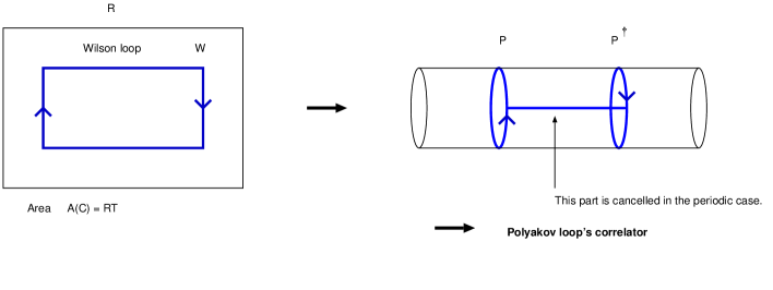
Figure 1: Polyakov loops’ correlator.   The expectation value of a Wilson loop $W$ is equivalent to a correlator of Polyakov loops $P$ and $P^{\dagger}$ in the case of the periodic boundary conditions.

4 Comments on Gauge Fixing and $U(1)$ Background

In this section, we comment on the relation between the phase transition mechanism and the $U(1)$ background. First, let us recall that we have chosen the $OSp(4|2)$ type MAG. This gauge spoils the chiral $SU(2)_{\rm L}\otimes SU(2)_{\rm R}$ symmetry which exists in the Feynman type gauge. Eventually, only the $SU(2)_{\rm L}$ symmetry survives and the $SU(2)_{\rm R}$ symmetry is lost in the MAG case. Then, we obtain a topological object “monopole” peculiar to the MAG and it is absent in the Feynman gauge. This is an $U(1)$ Abelian mopole. Because the chiral symmetry is broken, we would not be able to apply the KO criterion. However, we have the topological object in our hand. Monopoles are interpreted as instantons in the 2D theory reduced by the PS mechanism in this case. These play an important role in the confinement of the Wilson criterion[3]. It is also conjectured that these play a central role in the phase transition as well. In the above study, we saw that the phase structure of the TQFT sector was screened and only a confining phase can appear. However, in the case of the MAG, the information about the phase transition mechanism is encoded in the $U(1)$ background and the Berezinskii-Kosterlitz-Thouless (BKT) transition[15] occurs by the condensation of the topological object. This would be clarified after we integrate out the non-diagonal gauge components. That manipulation is based on the $U(1)$ Abelian dominance and really was done in the work[16]. Then, we can obtain an Abelian projected effective theory. This is just the $U(1)$ theory but is asymptotically free. When the scheme of the reformulation is applied to this $U(1)$ theory[12], the TQFT sector of it becomes a 2D $O(2)$ NLSM with a vortex solution. It is widely known that a BKT phase transition is induced by the condensation of the vortexes in this $O(2)$ NLSM. In this theory, by using parameterizations of the fields $U$ and ${\bf S}$

$$U(x)={\rm e}^{i\varphi(x)},~{}~{}{\bf S}(x)=(\cos\varphi(x),\sin\varphi(x)),$$ (4.1)

we obtain the TQFT sector of the effective $U(1)$ theory:

$$S_{\rm TQFT}=\frac{\pi}{g^{2}_{\rm YM}}\int d^{2}x\partial_{\mu}{\bf S}(x)\partial_{\mu}{\bf S}(x).$$ (4.2)

Also, the ${\bf S}$ obeys the boundary condition at finite temperature. But we can easily show that the boundary conditions on it becomes equivalent to the periodic ones when the perturbative parts are added. And so we cannot state the existence of the phase transition by the SSB in the TQFT sector as well. But, at least, we can find a BKT type phase transition by the $U(1)$ vortex condensation from the confining phase to the deconfining one. Moreover, it is commented in the work[16] that the $U(1)$ vortex is closely relevant to the instanton in the $O(3)$ NLSM. This possibly implies that the vortex condensation induces an instanton condensation and the confining potential would vanish. This would just correspond to the phase transition to the deconfining phase.

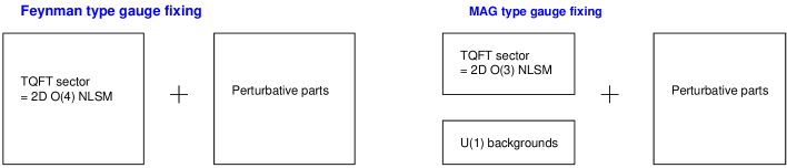
Figure 2: Comparison Feynman type gauge with MAG type gauge in $G=SU(2)$.   The phase structure of the TQFT sector is preserved in the case of the Feynman type gauge fixing. However, it is screened by the perturbative fluctuation in the case of the MAG type gauge fixing, and its information is encoded in the $U(1)$ backgrounds.

5 Discussion and Conclusion

We have investigated the effect of the boundary conditions and found that it depends on the gauge fixings. Because the analysis based on the KO criterion does not depend on the complicated dynamical information about the ${\rm QCD_{4}}$, we could not derive the mechanism of the confinement directly. On the other hand, when we choose the MAG, we can understand the dynamical mechanism in terms of monopoles. But because the analysis depends on the special gauge, we cannot know how reliable it is. Also, we could not discuss the Higgs phase. It is an interesting problem to study this phase by the use of the reformulation of ${\rm QCD_{4}}$

The phase structure of the ${\rm QCD_{4}}$ has investigated in the $OSp(4|2)$ type MAG and Feynman gauge. These investigations are based on the toy models where the special $OSp(4|2)$ type gauge fixing is utilized. But we could explain the results based on the KO criterion in the framework of the Wilson criterion, and believe that our considerations shed light on an interrelation between the works based on the KO criterion and those on the Wilson criterion. We hope the paper proceeds the understanding of the quark confinement.

Acknowledgements

The author would like to thank W. Souma for valuable discussions and K. Sugiyama for careful reading the manuscript and useful comments.

References

- [1] Y. Nambu, Phys. Rev. D 10, 4262 (1974).
- [2] S. Mandelstam, Phys. Rep. 23, 245 (1976).
- [3] K.-I. Kondo, Phys. Rev. D 58, 105019 (1998), hep-th/9801024.
-
[4]
H. Hata and Y. Taniguchi,
Prog. Theor. Phys. 94, 435 (1995), hep-th/9502083;
Prog. Theor. Phys. 93, 797 (1995), hep-th/9405145. - [5] K.I. Izawa, Prog. Theor. Phys. 90, 911 (1993).
- [6] T. Kugo and I. Ojima, Prog. Theor. Phys. Suppl. 66, 1 (1979).
- [7] R. Delbourgo and P.D. Jarvis, J. Phys. A 15, 611 (1982).
- [8] G. Parisi and N. Sourlas, Phys. Rev. Lett. 43, 744 (1979).
- [9] A.J. Niemi and G.W. Semenoff, Ann. Phys. 152, 105 (1984).
-
[10]
N.D. Mermin and H. Wagner, Phys. Rev. Lett. 17, 1133
(1966).
N.D. Mermin, J. Math. Phys. 8, 1061 (1967).
S. Coleman, Commun. Math. Phys. 31, 259 (1973). - [11] G.’t Hooft, Nucl. Phys. B 190, 455 (1981).
- [12] K.-I. Kondo, Phys. Rev. D 58, 085013 (1998), hep-th/9803133.
-
[13]
Y. Takahashi and H. Umezawa, Collective Phenomena 2,
55 (1975).
H. Umezawa, H. Matsumoto and M. Tachiki, “Thermo Field Dynamics and Condensed States” (North-Holland, Amsterdam, 1982). - [14] N.P. Landsman and Ch.G. van Weert, Phys. Report. 145, 141 (1987).
-
[15]
V.L. Berezinskii, Soviet Physics JETP 32, 493
(1971).
J.M. Kosterlitz, J. Phys. C 7, 1046 (1974).
J.M. Kosterlitz and D.V. Thouless, J. Phys. C 6, 1181 (1973). - [16] K.-I. Kondo, Phys. Lett. B 455, 251 (1999), hep-th/9810167; Phys. Rev. D 57, 7467 (1998), hep-th/9709109; Prog. Theor. Phys. Supplement, 131, 243 (1998), hep-th/9803063.