NEIP-00-012

DFTT 17/00

hep-th/0004183

The multiloop amplitudes for the bosonic string in presence of a constant $B$-field are built by using the basic commutation relations for the open string zero modes and oscillators. The open string Green function on the annulus is obtained from the one loop scattering amplitude among $N$ tachyons. For higher loops, it is necessary to use the so called three Reggeon vertex, which describes the emission from the open string of another string and not simply of a tachyon. We find that the modifications to the three (and multi) Reggeon vertex due to the $B$-field only affect the zero modes and can be written in a simple and elegant way. Therefore we can easily sew these vertices together and write the general expression for the multiloop $N$-Reggeon vertex, which contains any loop string amplitude, in presence of the $B$-field. The field theory limit is also considered in some examples at two loops and reproduces exactly the results of a noncommutative scalar field theory.

April, 2000

1 Introduction

It was Einstein’s remarkable idea that spacetime is dynamical and can be deformed by energy momentum tensor, with Riemannian geometry being the appropriate mathematical framework. It was realized recently that a constant $B$-field in string theory can also deform (D-brane worldvolume) spacetime [1, 3]. This kind of deformation is different from that of general relativity. In this case, the D-brane worldvolume becomes noncommutative. See [5] for a comprehensive introduction to noncommutative geometry.

The idea of noncommutative spacetime is not new. However, unlike the early approaches, the current developments of string theory display noncommutativity as a result of the underlying string or M-theory and do not require any further input. This has been clarified in [9, 13, 16, 18] for the string theory case, in [20] for the M-theory case and has also been extended in [22] for the charged string case.

Different directions of investigation have been undertaken since then. One direction is the study of the perturbative aspects [25]-[91] of noncommutative field theory, with the important discovery of UV/IR mixing [27]. Another interesting direction leaded by Alekseev, Recknagel and Schomerus [93] is the study of fuzzy physics for D-branes in WZW models [95].

There has also been a lot of interest recently [99, 101, 103, 105, 107] in exploring the relationships between noncommutative field theory and string theory. These studies have been partially motivated by the suggestion of [29] on the stringy origin of the UV/IR mixing, However, in all these works the 1-loop open string Green function is obtained from the closed string Green function by restriction to the boundary. This approach is indirect and there is no convincing reason that the closed string Green function should give rise to the open string Green function in this manner. One of the aims of the present paper is to settle this issue using only open string theory without resorting to closed string or comparison with field theory calculations.

In [13] the quantization of an open string in the presence of a $B$-field was carried out in the Hamiltonian formulation. One advantage of this approach is that the commutation relations for the modes of the string expansion are explicitly determined, with the noncommutativity of the string coordinates obtained as a derived concept. Therefore the results of [13] are particularly suitable for doing calculations in the operator formalism, where these commutation relations are essential. As we will review below, turning on a $B$-field has the effect of making the endpoints of open strings noncommutative. In terms of the commutation relations of the string expansion modes, it is a simple modification to the zero mode commutation relation (2.5), (2.9). This observation allows us to construct the open string vertex operators with $B$-field and determine the one-loop open string amplitudes directly. It is then straightforward to extract the one-loop open string Green function.

For higher loops, the approach of vertex operators becomes less useful. However the power of the operator formalism remains. One can uniformly construct higher loop string amplitudes by putting together (ie. sewing) the basic building blocks. The basic building blocks in this formalism are the BRST invariant open string propagator and three Reggeon vertex. Intuitively it can be expected that turning on a $B$-field does not modify the open string propagator. In fact, at field theory level, it is easy to see that the quadratic part of the action is unaffected by the noncommutative parameter and only the interaction terms depend on it. We show that a similar pattern is present also at string level. In this case, the interaction part can be summarized by the three Reggeon vertex; the modification of this vertex is again determined by the noncommutativity of the zero modes. By sewing a suitable number of three Reggeon vertices by means of propagators, we will build the generating functional for any $N$ point amplitude, called $N$-Reggeon vertex; we will find that, also in presence of $B$-field, it can be written down in an elegant and compact form at all loops.

The paper is organized as follows. In section 2, we construct the open string vertex operators with $B$-field and use them to compute the open string one loop amplitudes and extract the one-loop open string Green function. In section 3, we explain how $B$-field affects the basic building blocks in the construction of multiloop string amplitudes and obtain the $h$-loop $N$-point Reggeon vertex with $B$-field. In section 4, we consider the noncommutative $\Phi^{3}$ field theory in six dimensions at the two loops level and show that the field theory results agree precisely with the field theory limit of the two-loop string amplitudes we computed with the Reggeon vertex. We finally conclude with some open problems.

2 One-Loop Open String Green Function

In this section, we introduce the vertex operators for open string states in the presence of a constant $B$-field. Using these vertices, we can compute string amplitudes among tachyons states at tree and one-loop level; then, directly from this result, we extract the open string Green function on the annulus. As was recently shown, this is the basic ingredient for deriving noncommutative Feynman diagrams from string theory [99]–[107].

2.1 Open String Vertex Operator

We first recall the results [13] for an open string ending on a D-brane in presence of a constant $B$-field. Here, we will need only the open string coordinates in the longitudinal directions of the D-branes; in fact, for the purpose of deriving field theory diagrams from string amplitudes, it is sufficient to deal with spacetime filling D-branes. In this background the open string mode expansion is

$$X^{\mu}(\tau,\sigma)=x_{0}^{\mu}+2\alpha^{\prime}(p_{0}^{\mu}\tau-p_{0}^{\nu}F_{\nu}{}^{\mu}\sigma)+\sqrt{2\alpha^{\prime}}\sum_{n\neq 0}{e^{-{\rm i}n\tau}\over n}\bigl{(}{\rm i}a^{\mu}_{n}\cos n\sigma-a_{n}^{\nu}F_{\nu}{}^{\mu}\sin n\sigma\bigr{)}~{},$$ (2.1)

where $F=B-dA$ is the modified Born-Infeld field strength. In order to write the commutation relations of these modes, it is convenient to introduce the rescaled quantities

$$\hat{x}_{0}^{\mu}=x_{0}^{\nu}(1-F)_{\nu}{}^{\mu},\quad\hat{p}_{0}^{\mu}=p_{0}^{\nu}(1-F)_{\nu}{}^{\mu},\quad\hat{a}_{n}^{\mu}=a_{n}^{\nu}(1-F)_{\nu}{}^{\mu}~{}.$$ (2.2)

In fact, in terms of these operators, the equations take the standard form, except for that of the zero modes [13]

$$[\hat{a}_{n}^{\mu},\hat{x}_{0}^{\nu}]=[\hat{a}_{n}^{\mu},\hat{p}_{0}^{\nu}]=[\hat{p}_{0}^{\mu},\hat{p}_{0}^{\nu}]=0,$$ (2.3)

$$[\hat{a}_{m}^{\mu},\hat{a}_{n}^{\nu}]=m\eta^{\mu\nu}\delta_{m+n,0}~{},\quad[\hat{x}_{0}^{\mu},\hat{p}_{0}^{\nu}]={\rm i}\eta^{\mu\nu},$$ (2.4)

$$[\hat{x}_{0}^{\mu},\hat{x}_{0}^{\nu}]=2\pi{\rm i}\alpha^{\prime}F^{\mu\nu}={\rm i}\theta^{\mu\nu}~{}.$$ (2.5)

In the last line we have introduced the dimensionful quantity $\theta:=2\pi\alpha^{\prime}F$ which directly measures the noncommutativity. As we will see, this simple modification of the commutation relations for the zero mode $\hat{x}_{0}$ plays a fundamental role in giving the whole $\theta$-dependence of the string amplitude. We also recall that the normal-ordered Virasoro generators, defined in terms of the hatted operators, satisfy the standard Virasoro algebra (first paper in [13]) with a central charge unmodified by $F$.

The vertex operators for open string states emitted at the boundary are constructed using $\hat{X}^{\mu}$ evaluated at $\sigma=0$ or $\sigma=\pi$,

$$\hat{X}^{\mu}(\tau,0) = \hat{x}_{0}^{\mu}+2\alpha^{\prime}\hat{p}_{0}^{\mu}\tau+{\rm i}\sqrt{2\alpha^{\prime}}\sum_{n\neq 0}{e^{-{\rm i}n\tau}\over n}\hat{a}^{\mu}_{n}~{},$$ (2.6)

$$\hat{X}^{\mu}(\tau,\pi) = \hat{y}_{0}^{\mu}+2\alpha^{\prime}\hat{p}_{0}^{\mu}\tau+{\rm i}\sqrt{2\alpha^{\prime}}\sum_{n\neq 0}\frac{(-e^{-{\rm i}\tau})^{n}}{n}\hat{a}^{\mu}_{n}~{},$$

where we have introduced

$$\hat{y}_{0}^{\mu}:=\hat{x}_{0}^{\mu}-2\alpha^{\prime}\pi\hat{p}_{0}^{\nu}F_{\nu}{}^{\mu}~{}.$$ (2.7)

The zero-mode $\hat{y}_{0}$, appearing in the expansion of $\hat{X}^{\mu}(\tau,\pi)$, satisfies

$$[\hat{x}_{0}^{\mu},\hat{y}_{0}^{\nu}]=0,$$ (2.8)

$$[\hat{y}_{0}^{\mu},\hat{y}_{0}^{\nu}]=-{\rm i}\theta^{\mu\nu}.$$ (2.9)

For instance, the open string tachyon vertex operator for emission at $\sigma=0$ is

$$V(p,\tau) = :e^{{\rm i}p\cdot\hat{X}(\tau,0)}:~{}$$

$$= \exp\left(\sqrt{2\alpha^{\prime}}\;p\cdot\sum_{n=1}^{\infty}\frac{\hat{a}_{-n}}{n}e^{{\rm i}n\tau}\right)\;e^{{\rm i}p\cdot\hat{x}_{0}}e^{{\rm i}2\alpha^{\prime}p\cdot\hat{p}_{0}\tau}\;\exp\left(-\sqrt{2\alpha^{\prime}}\;p\cdot\sum_{n=1}^{\infty}\frac{\hat{a}_{n}}{n}e^{-{\rm i}n\tau}\right)~{},$$

while, for the emission at $\sigma=\pi$, we just have to replace $\hat{x}_{0}$ by $\hat{y}_{0}$ in the above. It is straightforward to check that it satisfies the desired property, both for $\sigma=0$ and $\sigma=\pi$

$$[L_{m},V(p,\tau)]=e^{im\tau}(-{\rm i}\frac{d}{d\tau}+\frac{1}{2}mp^{2})V(p,\tau)~{}.$$ (2.11)

Similarly, one can construct the vertex operators for higher open string states. For example, the gluon vertex operator is

$$V_{\varepsilon}(p,\tau)=\varepsilon\cdot\frac{d\hat{X}}{d\tau}~{}e^{ip\cdot\hat{X}}\;.$$ (2.12)

We want to stress that the commutation relation (2.9) has an opposite sign compared to (2.5). This is in agreement with the result of [13] where it was shown that

$$[\hat{X}^{\mu}(\tau,\sigma),\hat{X}^{\nu}(\tau,\sigma^{\prime})]=\left\{\begin{array}[]{ll}\pm i\theta^{\mu\nu},&\sigma=\sigma^{\prime}=0\mbox{ or }\pi,\cr 0,&\mbox{otherwise},\end{array}\right.$$ (2.13)

This means that the noncommutativity of the string coordinates $\hat{X}^{\mu}$ at equal time is entirely determined by the zero modes. Note that (2.13) is equivalent to say that multiplication for functions defined on the D-brane worldvolume are done in opposite ordering (sec. 5 of first paper in [13] and sec. 6.2 of [18]). This difference in the commutation relation for $\hat{x}_{0}$ and $\hat{y}_{0}$ is not so important for tree level calculations, since one can choose to put all interactions at $\sigma=0$. However, this difference becomes essential for one-loop diagrams: in fact, in this case non-planar diagrams require to put vertex operators at the two different borders, $\sigma=0$ and $\sigma=\pi$.

Finally, we remark that the vertex operator $V_{\alpha}(p,\tau)$ for a string state $\alpha$ satisfies

$$V_{\alpha_{1}}(p_{1},\tau_{1})V_{\alpha_{2}}(p_{2},\tau_{2})=V_{\alpha_{2}}(p_{2},\tau_{2})V_{\alpha_{1}}(p_{1},\tau_{1})e^{i\phi},$$ (2.14)

where

$$\phi=\left\{\begin{array}[]{c@{}cl}&2\pi\alpha^{\prime}\;p_{1}\cdot p_{2}\;\epsilon(\tau_{1}-\tau_{2})-p_{1}\,\theta\,p_{2}~{},&\mbox{if $\alpha_{1}$ and $\alpha_{2}$ are on the same border $\sigma=0$},\cr&-2\pi\alpha^{\prime}\;p_{1}\cdot p_{2}\;\epsilon(\tau_{1}-\tau_{2})+p_{1}\,\theta\,p_{2}~{},&\mbox{if $\alpha_{1}$ and $\alpha_{2}$ are on the same border $\sigma=\pi$},\cr&0,&\mbox{if $\alpha_{1}$ and $\alpha_{2}$ are on different borders, }\end{array}\right.$$ (2.15)

and $\epsilon(\tau)=\tau/|\tau|$. The $\theta$-dependent piece is a simple consequence of the zero mode commutation relations (2.5), (2.8) and (2.9) and of the fact that either the zero mode $\hat{x}_{0}$ or $\hat{y}_{0}$ appears in the vertex, depending on whether it is on the $\sigma=0$ or $\sigma=\pi$ border. The difference of sign for the two borders in (2.15) is crucial, since it ensures that tree-level string amplitudes are invariant under cyclic permutations. For instance, it is easy to work out the $N$-point amplitude, where some of the legs are emitted from the border $\sigma=0$ and the others from $\sigma=\pi$, and then to verify that the result is cyclically invariant: one has simply to use the commutation relation (2.14) and momentum conservation. In Fig 1, vertices inserted on the $\sigma=0$ ($\sigma=\pi$) boundary are represented by a vertical line above (below) the horizontal line.

Figure 1: Cyclicity of the tree level $N$-Reggeon vertex.

2.2 Open String Green Function

Now we compute the 1-loop open string amplitude for tachyons using the vertex operators constructed above and extract the open string Green function from it. Consider the $M+N$-point amplitude depicted in Fig. 2.

Figure 2: One annulus in Schottky representation.

The external states $n\in\{1,\cdots,M\}:=I_{1}$ are on the boundary $\sigma=0$, while the other particles $s\in\{M+1,\cdots,M+N\}:=I_{2}$ are on the boundary $\sigma=\pi$; moreover, we have chosen the radial ordering

$$k\leq|\rho_{M+N}|\cdots\leq|\rho_{M+1}|\leq\rho_{M}\cdots\leq\rho_{2}\leq\rho_{1}\leq 1.$$ (2.16)

The 1-loop amplitude is given by

$$A(1,\ldots,M;M+1,\ldots,M+N)\sim\int d^{d}p\;{\rm tr}\Big{\{}V(p_{1},\rho_{1})\ldots V(p_{M+N},\rho_{M+N})\,k^{L_{0}}\Big{\}},$$

where $V$ is the vertex introduced in (2.1). First we look at the part containing $\hat{x}_{0}$ and $\hat{y}_{0}$, which is given by

$$e^{{\rm i}p^{1}\hat{x}_{0}}\ldots\,e^{{\rm i}p^{M}\hat{x}_{0}}e^{{\rm i}p^{(M+1)}\hat{y}_{0}}\ldots\,e^{ip^{(M+N)}\hat{y}_{0}}\\ =e^{-{\rm i}\hat{p}_{0}\theta\sum_{s\in I_{2}}p^{s}}e^{-\frac{i}{2}\sum_{\stackrel{{\scriptstyle r<s}}{{r,s\in I_{1}}}}p^{r}\theta p^{s}}e^{\frac{i}{2}\sum_{\stackrel{{\scriptstyle r<s}}{{r,s\in I_{2}}}}p^{r}\theta p^{s}}~{}.$$

Evaluating the trace turns $\hat{p}_{0}$ into the loop momentum $p$. Notice that, besides the usual $p$ dependent factors coming from the propagators, one has a new term linear both in $\theta$ and in $p$ which has its origin in the commutation relations of the zero modes $\hat{x}_{0}$ and $\hat{y}_{0}$ . Globally the zero mode part becomes

$$\int d^{d}p\,\exp\left(\alpha^{\prime}p^{2}\ln k+p\cdot\Bigg{(}2\alpha^{\prime}\!\!\sum_{r\in I_{1}\cup I_{2}}\!\!p^{r}\ln|\rho_{r}|-{\rm i}\theta\sum_{s\in I_{2}}p^{s}\Bigg{)}-\alpha^{\prime}\!\!\!\!\!\sum_{\stackrel{{\scriptstyle r<s}}{{r,s\in I_{1}\cup I_{2}}}}\!\!\!p^{r}\cdot p^{s}\ln\left|\frac{\rho_{s}}{\rho_{r}}\right|\right).$$ (2.17)

The Gaussian integration over $p$ is performed, as usual, by completing the square; in particular, the expression in the exponent is equal to

$$\alpha^{\prime}\ln k\left[p+\frac{1}{\ln k}\Bigg{(}\sum_{r\in I_{1}\cup I_{2}}p^{r}\ln|\rho_{r}|-{\rm i}\frac{\theta}{2\alpha^{\prime}}\sum_{s\in I_{2}}p^{s}\Bigg{)}\right]^{2}+\alpha^{\prime}\!\!\!\!\!\sum_{\stackrel{{\scriptstyle r<s}}{{r,s\in I_{1}\cup I_{2}}}}\!\!\!p^{r}\cdot p^{s}\Bigg{(}\frac{\ln^{2}|\rho_{s}/\rho_{r}|}{\ln k}-\ln\left|\frac{\rho_{s}}{\rho_{r}}\right|\Bigg{)}$$

$$+\frac{1}{\alpha^{\prime}\ln k}\sum_{r\in I_{1},s\in I_{2}}p^{r}\left(\frac{\theta}{2}\right)^{2}p^{s}+\frac{{\rm i}}{\ln k}\sum_{r\in I_{1}\cup I_{2}}\;\sum_{s\in I_{2}}\ln|\rho_{r}|p^{r}\theta p^{s}~{}.$$ (2.18)

It is easy to see that the last term in the above equation is equal to

$$\frac{{\rm i}}{\ln k}\sum_{r\in I_{1},s\in I_{2}}\ln|{\rho_{r}}{\rho_{s}}|p^{r}\theta p^{s}.$$ (2.19)

The momentum integral can now be evaluated and the second line of (2.18) contains two new terms arising in nonplanar diagrams. In the non zero-modes part, the extra minus sign in front of the $\hat{a}_{n}$ oscillators in the $\hat{X}(\pi)$ expansion has the effects to change the sign of $\rho$ in the oscillator sum for the nonplanar vertices. It is worthwhile to remark again that the $\theta$ and $\theta^{2}$ terms above arise as a result of the new linear $p$-shift in the Gaussian integration. We will see that the same pattern repeats for the general case of the $h$-loop Reggeon vertex.

Finally we can summarize 1-loop amplitudes in the following compact equation

$$A(1,\!\!\!\! \ldots, \!\!\!\!M;M+1,\ldots,M+N)\sim\int\limits_{0}^{1}\frac{dk}{k^{2}}\left(\frac{-2\pi}{\ln k}\right)^{d/2}(1-k^{n})^{2-d}\int\frac{d\rho_{2}}{\rho_{2}}\cdots\frac{d\rho_{M+N}}{\rho_{M+N}}$$ (2.20)

$$\prod_{\stackrel{{\scriptstyle r<s}}{{r,s\in I_{1}}}}e^{2\alpha^{\prime}G_{P}^{\mu\nu}(\rho_{r},\rho_{s})p^{r}_{\mu}p^{s}_{\nu}}\prod_{r\in I_{1},s\in I_{2}}e^{2\alpha^{\prime}G_{NP}^{\mu\nu}(\rho_{r},\rho_{s})p^{r}_{\mu}p^{s}_{\nu}}\prod_{\stackrel{{\scriptstyle r<s}}{{r,s\in I_{2}}}}e^{2\alpha^{\prime}G_{P}^{\mu\nu}(\rho_{r},\rho_{s})p^{r}_{\mu}p^{s}_{\nu}}~{},$$

where the planar and nonplanar open string Green function are

$$G_{P}^{\mu\nu}(\rho,\rho^{\prime})=I_{0}^{P}\eta^{\mu\nu}-\frac{{\rm i}\theta^{\mu\nu}}{4\alpha^{\prime}}\epsilon(\rho-\rho^{\prime})\;,\!\quad G_{NP}^{\mu\nu}(\rho,\rho^{\prime})=I_{0}^{NP}\eta^{\mu\nu}+\frac{(\theta^{2})^{\mu\nu}}{8\alpha^{\prime 2}}\frac{1}{\ln k}\pm\frac{{\rm i}\theta^{\mu\nu}}{2\alpha^{\prime}}\frac{\ln|\rho\rho^{\prime}|}{\ln k},$$ (2.21)

with the $\theta$-independent piece $I_{0}$ given by

$$I_{0}^{P}(\rho,\rho^{\prime})=\frac{\ln^{2}\rho/\rho^{\prime}}{2\ln k}+\ln\left|\sqrt{\frac{\rho}{\rho^{\prime}}}-\sqrt{\frac{\rho^{\prime}}{\rho}}\right|+\ln\prod_{n=1}^{\infty}\left|\frac{(1-k^{n}\rho/\rho^{\prime})(1-k^{n}\rho^{\prime}/\rho)}{(1-k^{n})^{2}}\right|$$ (2.22)

for the planar case, while for nonplanar contractions one has

$$I_{0}^{NP}(\rho,\rho^{\prime})=\frac{\ln^{2}|\rho/\rho^{\prime}|}{2\ln k}+\ln(\sqrt{\frac{|\rho|}{|\rho^{\prime}|}}+\sqrt{\frac{|\rho^{\prime}|}{|\rho|}})+\ln\prod_{n=1}^{\infty}\left|\frac{(1+k^{n}|\rho/\rho^{\prime}|)(1+k^{n}|\rho^{\prime}/\rho|)}{(1-k^{n})^{2}}\right|~{}.$$ (2.23)

In the last term of the nonplanar Green function in (2.21), positive sign is taken when $\rho>0,\rho^{\prime}<0$ and negative sign is taken for the opposite case $\rho^{\prime}>0,\rho<0$. This follows directly from our result (2.19).

By using these Green functions, one can compute different string amplitudes that, in the limit $\alpha^{\prime}\to 0$, reproduce the Feynman diagrams of diverse noncommutative field theory. For example, by introducing in (2.20) the Schwinger parameters $t_{i}~{}(2\leq i\leq M+N$)

$$-\alpha^{\prime}\ln|\rho_{k}|=t_{2}+t_{3}+\cdots+t_{k},\quad 2\leq k\leq M+N,$$ (2.24)

and taking $\alpha^{\prime}\rightarrow 0$ with $\theta=2\pi\alpha^{\prime}F$ and $t_{i}$ both kept fixed, the result is precisely the same as the corresponding noncommutative $\Phi^{3}$ field theory amplitude, derived by means of the noncommutative Feynman rules. This provides an independent field theory check of the correctness of the string computation (2.20) and of the vertex operators we constructed above. By contracting some of the propagators [103], one can also obtain from (2.20) other field theory limits, for example noncommutative $\Phi^{4}$.

We note that, in the tachyon amplitudes (2.20), the Green functions are always contracted with the external momenta. Because of this, it is also possible, by using momentum conservation, to rewrite the last term of (2.18) as a function of the ratio of the $\rho$’s over the two borders,

$$-\frac{{\rm i}}{\ln k}\left(\sum_{\stackrel{{\scriptstyle r<r^{\prime}}}{{r,r^{\prime}\in I_{1}}}}\ln\left|\frac{\rho_{r}}{\rho_{r^{\prime}}}\right|p^{r}\theta p^{r^{\prime}}-\sum_{\stackrel{{\scriptstyle s<s^{\prime}}}{{s,s^{\prime}\in I_{2}}}}\ln\left|\frac{\rho_{s}}{\rho_{s^{\prime}}}\right|p^{s}\theta p^{s^{\prime}}\right)~{}.$$ (2.25)

This shows explicitly that the tachyon amplitude is invariant under the transformation

$$\rho_{s}\to\lambda\rho_{s},\quad\mbox{and}\quad\rho_{s}\to-\lambda/\rho_{s},\quad\lambda>0.$$ (2.26)

It is easy to generalize the manipulations here and to show that this is also true for the gluon amplitudes as well as the amplitudes for other higher string states.

We also remark that written in the form (2.25), one may shift this piece to the planar diagram and extract a different planar and nonplanar Green function

$$G^{\prime\mu\nu}_{P}=I_{0}^{P}\eta^{\mu\nu}-\frac{{\rm i}\theta^{\mu\nu}}{4\alpha^{\prime}}\epsilon(\rho-\rho^{\prime})\mp\frac{{\rm i}\theta^{\mu\nu}}{2\alpha^{\prime}\ln k}\ln\left|\frac{\rho}{\rho^{\prime}}\right|,\quad\quad G^{\prime\mu\nu}_{NP}=I_{0}^{NP}\eta^{\mu\nu}+\frac{(\theta^{2})^{\mu\nu}}{8\alpha^{\prime 2}}\frac{1}{\ln k}.$$ (2.27)

where $-$ sign is for the positive border and $+$ sign is for the negative border. Incidentally, these are the same as one obtained from restricting to the boundary of the 1-loop closed string Green function [99]. However, as stressed in [103], (2.21) and (2.27) are not equivalent when one wants to deal with external massless states and derive, for instance, the Feynman diagrams of the noncommutative gauge theory. Indeed the necessity of shifting the result naturally obtained from the closed string calculations is clear within string theory, without the need to refer to any field theory results. For instance, by following the same procedure of this section, one can compute a general 1-loop gluon interaction if the vertex operator (2.12) are used instead of (2.1). Then one has to rewrite the final amplitude in the form of the string master formula for gluons, and identify the Green function from it. The result is indeed given by (2.21), (2.22) above, naturally derived also in the scalar computation.

3 Reggeon Vertex and Multiloop String Amplitudes

In this section we first construct the tree-level BRST invariant $N$-Reggeon vertex for open bosonic string in presence of a constant $B$-field. This object is the generator of all tree-level scattering amplitudes among arbitrary string states and will provide the first basic ingredient for constructing higher loop “noncommutative” string diagrams. It is quite clear why it is necessary, for our purposes, to introduce the Reggeon vertex formalism. As usual, in order to construct loop amplitudes, one sews together pairs of external legs and sums over all contributions coming from the exchange of the different string states in the various loops. In the previous section this has been achieved by simply identifying the first ($z=\infty$) and the last ($z=0$) leg and then taking the trace. This approach is no longer adequate for constructing higher loop amplitudes; in fact, in order to repeat the sewing procedure, we need to identify further couples of legs that cannot be fixed at $z=0$ and $z=\infty$. However, in the vertex operator formalism, all these legs have been represented by vertex operators describing specific string states and thus it is very difficult to sum the contributions coming from the exchange of different states. As we will briefly review, the introduction of Reggeon vertex solves this problem.

The second fundamental ingredient that is necessary for constructing higher loop interactions is the BRST invariant open string propagator. From the geometrical point of view, this propagator is a conformal transformation identifying two circles around the punctures sewn together. It turns out that this ingredient is not modified by the presence of a constant $B$-field. Thus the $B$-dependent $N$-Reggeon vertex will be the only new building block we need to use for computing the “noncommutative” string amplitudes at loop level.

3.1 Tree level Reggeon Vertex

The starting point is a generalization of the usual vertices describing the emission of string states. As is clear by looking at the simplest case (2.1), these vertices are built by means of the coordinates of the propagating virtual string and their explicit form is determined by the quantum numbers of the emitted states like momentum or polarizations. In the generalization of these usual vertices, one basically replaces [109] the quantum numbers of the emitted string with a whole Hilbert space. Thus, considering also the ghost contribution, the $3$-Reggeon vertex is [112] 

$$V_{3;0}^{\theta}(\zeta)=\langle 0;q=3|:\exp\left\{\oint_{0}dz(-X^{v}(\zeta+z)\partial_{z}X(z)-c^{v}(\zeta+z)b(z)+b^{v}(\zeta+z)c(z))\right\}:~{},$$ (3.1)

where the bra indicates the vacuum of the emitted string for both the oscillators and the zero mode $x_{0}$, while the label $q=3$ specifies the ghost number

$$|0;q=3\rangle=|x_{0}=0;0_{a}\rangle\otimes c_{-1}c_{0}c_{1}|q=0\rangle~{}.$$ (3.2)

Besides the fields of the virtual string denoted by $v$, in the $3$-Reggeon vertex, also the coordinates of the external string appear directly; the commutations relations of these new modes are the usual ones (2.3)–(2.5), while the oscillators of the virtual and the external strings simply commute among them. Formally our expression is identical to the one normally used in string calculation in the trivial background $B=0$; however, (3.1) depends on the value of the $B$-field through the mode expansion (2.6) and the new commutation relations, which have to be used both for the virtual and the external string. Here for convenience, we have dropped the hat over the $X$ fields, although it should be understood that all the $X$’s above contain the oscillators defined in (2.2). Notice that, in terms of the rescaled coordinates, the zero-mode $x_{0}$ (or $y_{0}$ if the interaction is at $\sigma=\pi$) appears only in the expansion of the virtual string and is the only source of the non-trivial dependence on $\theta$. Together with the Reggeon vertex (3.1), we will employ the usual physical states having ghost number $1$; thus, the $(b,c)$ system is not affected by the background field $F$ and one recovers the well known results for ghosts. Because of this, in what follows, we will no longer mention ghosts and focus only on the $F$-dependent modifications coming from the orbital part.

The key property of the 3-Reggeon vertex is that it can be saturated with a string state $\alpha$ and one recovers the usual vertex operator corresponding to the considered state

$$V_{3;0}^{\theta}(\zeta)|p;\alpha\rangle=V_{\alpha}(p,\zeta)~{}.$$ (3.3)

It is easy to check that when completely saturated with external states, the 3-Reggeon vertex gives correctly the tree level amplitude, including the phase factor

$${{}_{v}}\langle p_{1};\alpha_{1}|~{}V_{3;0}^{\theta}~{}|p_{2};\alpha_{2}\rangle\;|p_{3};\alpha_{3}\rangle_{v}\sim{\rm e}^{\mp\frac{i}{2}p^{1}\theta p^{2}}~{},$$ (3.4)

where, again, the upper (lower) sign refers to the emission of the particle $\alpha_{2}$ from the border $\sigma=0$ ($\sigma=\pi$) of the propagating string $v$; in particular, the phase arises because of the use of the commutation relation (2.5) (or (2.9)) for the zero modes.

We remark that all the formula written in this section are general and hold for any value of $\alpha^{\prime}$. In the next section, we will consider the noncommutative field theory limit

$$\alpha^{\prime}\to 0,\quad F\to\infty$$ (3.5)

with $\alpha^{\prime}F$ fixed so that a noncommutative field theory is obtained.

The tree level $N$-Reggeon vertex can be constructed simply by multiplying $N$ $3$-Reggeon vertices in different positions $\zeta$, but written in terms of the same propagating string $v$. Then, one can explicitly evaluate the vacuum expectation value in the Hilbert space $v$ in order to keep only the dependence on the oscillators of the external states. The new $\theta$-dependent part comes when one collects together the zero mode factors. In particular, if the external legs of all the original 3-Reggeon vertices are emitted from the border $\sigma=0$, one obtains the new phase factor

$$e^{ip^{1}x_{0}}\cdots e^{ip^{N}x_{0}}=e^{-\frac{i}{2}\sum_{r<s}^{N}{p}^{r}\theta{p}^{s}},$$ (3.6)

where momentum conservation has been used. As a result, we obtain the $N$-Reggeon vertex with all legs emitted from the $\sigma=0$ border

$$V_{N;0}^{\theta}=V_{N;0}^{0}\exp(-\frac{i}{2}\sum_{i<j}^{N}{p}^{i}\theta{p}^{j}),$$ (3.7)

where ${p}^{i}$ is the momentum operator of the $i$-th leg, in the direction flowing towards the boundary. Here $V_{N;0}^{0}$ indicates the $N$-Reggeon vertex derived for the usual “commutative” case $F=0$ in [114, 115]. This vertex is a bra in the direct product of the $N$ distinct Fock spaces for the external strings; like the $3$-Reggeon vertex, it gives the scattering amplitude when the external legs are saturated with physical states. In particular, like the 3-Reggeon vertex, $V_{N;0}^{0}$ contains the vacuum of the zero modes

$$\prod_{i=1}^{N}\;\langle x_{0}^{i}=0|=\prod_{i=1}^{N}\int dp^{i}\;\langle p^{i}|.$$ (3.8)

The momentum operator dependent phase factor in (3.7) is to be interpreted as an operator acting on the R.H.S. of (3.8). When saturated with external states, it gives a (numerical) phase factor as the $p^{i}$’s become the external momenta. In the next section, we will sew together legs of the tree level Reggeon vertex (3.7) to construct the multiloop Reggeon vertex. We will see that the momenta of the corresponding legs are to be identified and interpreted as the loop momentum. (3.8) effectively instructs us to integrate over the loop momentum.

We also note that the only modification to the tree level $N$-point vertex is the momentum dependent phase factor. This is exactly the same kind of modification to the tree level vertex in a noncommutative field theory due to the Moyal $*$-product. We will see that this identification of the modifications in the string vertex and field theory vertex is the basic reason which guarantees that the usual one-one correspondence between corners of string moduli space and field theory Feynman diagrams continues to hold in the noncommutative case.

3.2 $h$-loop $N$-Reggeon Vertex

The $h$-loop $N$-Reggeon vertex in the presence of a constant $F$-field can be constructed by sewing together legs of a tree level ($N+2h$)-Reggeon vertex. For example, in order to sew together leg $2$ and leg $(N-1)$, we identify the corresponding Fock spaces

$$a_{n}^{(2)}\to a_{n}^{(N-1)\dagger},\quad p^{(2)}\to-p^{(N-1)},$$ (3.9)

$$b_{n}^{(2)}\to b_{n}^{(N-1)\dagger},\quad\quad c_{n}^{(2)}\to-c_{n}^{(N-1)\dagger}.$$ (3.10)

The next step in the sewing procedure is to identify the punctures of the legs that are going to be sewn together. In terms of local coordinates $V_{i}^{-1}$ around the puncture $z_{i}$, this means we have to identify $V_{i}^{-1}(z)$ and $V_{j}^{-1}(z)$ so that a complex structure can still be defined. In (3.1), we have chosen for the sake of simplicity $V_{i}(z)=z+z_{i}$. However, the $N$-Reggeon vertex can be written for general conformal transformation $V_{i}$’s and it is easy to check that the string amplitude is independent of the choice of them. Because of this arbitrariness in the choice of the $V_{i}$, there are in general many more redundant variables in the Reggeon vertex than in the physical amplitudes. It is therefore useful to make some convenient choices on the $V_{i}$’s so as to obtain a simpler expression for the Reggeon vertex in order to simplify intermediate calculations and manipulations. In particular, for constructing higher loop amplitudes through the sewing procedure, the Lovelace choice [116] is useful. In this choice, $V_{i}$ is a projective transformation which maps $\infty,0,1$ to $z_{i-1},z_{i},z_{i+1}$. The sewing is achieved by using the BRST invariant sewing operator $P(x)$ [115], which is a function of $L_{0}$ and $L_{\pm 1}$ and of the ghosts. Since $L_{n}$ does not involve the zero modes $x_{0}$, we conclude that the string propagator $P(x)$ and the sewing procedure are not modified by the presence of $F$-field. Therefore the only new feature for $\theta\neq 0$ is in the zero modes part of the Reggeon vertex.

Fig 3 shows how to construct a $N$-Reggeon vertex with all legs emitted on the border $\sigma=0$.

Figure 3: A Reggeon vertex with external momenta $p_{1},p_{2}$ crossing an internal momentum.

As we have already said the ghost system is not modified by the $F$-field, thus its contribution (both zero and nonzero modes) to the Reggeon vertex is unchanged. Using (3.7) and recalling (3.8), it is straightforward to show that the $h$-loop $N$-Reggeon vertex in the presence of $F$-field is

$$V_{N;h}^{\theta}=\widetilde{V}_{N;h}^{0}\prod_{I=1}^{h}\int dp^{I}\exp\left(\frac{1}{2}\sum_{I,J=1}^{h}p^{I}_{\mu}A_{IJ}^{\mu\nu}p^{J}_{\nu}+\sum_{I=1}^{h}B_{I}^{\mu}p^{I}_{\mu}+C\right),$$ (3.11)

where $\widetilde{V}_{N;h}^{0}$ contains the ghost contribution and only the nonzero mode piece of the orbital part of $N$-Reggeon vertex in absence of background. Its explicit form can be found in [117, 114]. What interests us is that all the dependence in $\theta$ is localized in the zero modes loop momentum integration. We obtain the following modifications to $A,B,C$

$$A_{IJ}^{\mu\nu}={A^{0}}_{IJ}^{\mu\nu}-i\theta^{\mu\nu}\cal J_{IJ},$$ (3.12)

$$B_{I}^{\mu}={B^{0}}_{I}^{\mu}-i\theta^{\mu\nu}{P}_{I\nu},$$ (3.13)

$$C=C^{0}-\frac{i}{2}\sum_{i<j}^{N}{p}^{i}\theta{p}^{j},$$ (3.14)

where $p_{I}$, $I=1,\cdots h$ are the loop momenta; $p_{i}$, $i=1,\cdots,N$ are the external momenta; $\cal J_{IJ}$ is the intersection matrix for the internal loops; $P_{I}$ is the sum of external momentum entering the $I^{th}$ loop. For example in Fig 3, it is

$$P_{1}=p_{1}+p_{2},\quad P_{2}=0.$$ (3.15)

The explicit form of $A,B,C$ for $\theta=0$ are given in [117],

$${A^{0}}_{IJ}^{\mu\nu} = 2\alpha^{\prime}(2\pi i\tau_{IJ})\delta^{\mu\nu},$$ (3.16)

$${B^{0}}_{I}^{\mu} = \frac{1}{2\pi}\sum_{i=1}^{N}\oint_{0}dz\partial X^{(i)\mu}(z)\int_{z_{0}}^{V_{i}(z)}\omega_{I}~{},$$ (3.17)

$$C^{0} = -\frac{1}{2}\sum_{i=1}^{N}\oint_{0}dz\partial X^{(i)}(z)p_{0}^{(i)}\ln V^{\prime}_{i}(z)$$

$$+\frac{1}{2\alpha^{\prime}}\sum_{i<j}^{N}\oint_{0}dz\oint_{0}dy\partial X^{(i)}(z)\ln[V_{i}(z)-V_{j}(y)]\partial X^{(j)}(y)$$

$$+\frac{1}{4\alpha^{\prime}}\sum_{i,j=1}^{N}\oint_{0}dz\oint_{0}dy\partial X^{(i)}(z)\ln\left(\frac{E(V_{i}(z),V_{j}(y))}{V_{i}(z)-V_{j}(y)}\right)\partial X^{(j)}(y).$$

Here $V_{i}(z)$ is chosen to satisfy $V_{i}^{-1}(z)=0$ for $z=z_{i}$. $\omega_{I}$ is the normalized Abelian differential,

$$\oint_{a_{J}}\omega_{I}=\delta_{IJ}$$ (3.19)

and

$$2\pi i\tau_{IJ}=\oint_{b_{J}}\omega_{I}$$ (3.20)

is the period matrix and $E(z,w)$ is the prime form. Their explicit expressions in term of the Schottky parameters can be found in [117]. One can easily carry out the integration over $z$ in the above expressions

$${1\over 2\pi}\oint_{0}dz\partial X(z)f(z)=2\alpha^{\prime}pf(0)+\sqrt{2\alpha^{\prime}}\sum_{n=1}\frac{a_{n}}{n!}\partial^{n}f(z)|_{z=0}$$ (3.21)

and explicitly rewrite ${B^{0}}_{I}^{\mu}$ and $C^{0}$ in terms of modes. In particular, one finds here (and in the following (3.24), (3.26) and (3.2)) terms containing only the zero modes $p$. In this case, the arguments of the log’s must be taken in absolute value. This absolute value has its origin in the matrix element $D_{00}=(1/2)\log|\gamma^{\prime}(0)|$ of the real infinite dimensional representation of the projective group, relevant for the open string (see ref. [115]).

A couple of remarks are in order. The modification in (3.14) is the universal phase factor depending on the external momentum. It corresponds to the Filk phase [25] in the field theory limit. The $\theta$-dependent shift in (3.13) corresponds in the field theory limit to the shift due to the dipole mechanism [39, 41, 65]. The string theory interpretation of this shift in terms of stretched string was recently discussed in [107]. The shift in (3.12) is new and, among other effects, gives rise to a $\theta$ dependent measure factor for the zero modes of the orbital degrees of freedom. One obvious advantage of our approach is the clarity of the modifications due to $B$-field to the multiloop string amplitudes: it is summarized in the zero mode contributions in (3.22). As a result, apparently unrelated field theory effects could find a uniform string explanation.

Carrying out the loop momentum integration, we obtain finally

$$V_{N;h}^{\theta}=\widetilde{V}_{N;h}^{0}\frac{1}{\sqrt{{\rm det\,}\frac{-A}{2}}}\exp(-\frac{1}{2}B^{T}A^{-1}B+C),$$ (3.22)

where the determinant is taken over the space of Lorentz and loop indices $(\mu I)$. When $\theta=0$, it is

$$\sqrt{{\rm det\,}(-A/2)}=({\rm det\,}(-2\pi i\alpha^{\prime}\tau))^{d/2}.$$ (3.23)

It is remarkable that the multiloop string amplitudes can again be written in terms of geometrical quantities of the Riemann surface like the first Abelian differentials, period matrix and the prime form, together with the intersection matrix of the loops.

Finally we close this section by writing down explicitly the $\theta$-dependences in the Reggeon vertex for the one loop case. First, there is no modification to ${A^{0}}_{IJ}^{\mu\nu}$ and the modification to $C^{0}$ is simply the usual field theory Filk phase. Thus we concentrate on the effects from the shift of ${B^{0}}^{\mu}_{I}$. The one-loop Abelian differential is $\omega=dz/z$. With the convenient choice of $V_{i}(\rho)=\rho+\rho_{i}$, we have

$${B^{0}}_{I}^{\mu}=\sum_{r\in I_{1}\cup I_{2}}{\cal B}^{r\,\mu}(\rho)\ln(\rho+\rho_{r}),$$ (3.24)

where

$${\cal B}^{r\,\mu}(\rho)=\frac{1}{2\pi}\oint_{0}d\rho\partial X^{(r)\mu}(\rho)$$ (3.25)

is an operator in which the integration in carried out on any function that multiply ${\cal B}$ on the right. Since $P=\sum_{s\in I_{2}}p^{s}=\sum_{s\in I_{2}}{\cal B}^{s}$ for the only loop we have, it is

$$B^{0\mu}-i\theta^{\mu\nu}P_{\nu}=\sum_{r\in I_{1}\cup I_{2}}{\cal B}^{r\,\mu}(\rho)\ln(\rho+\rho_{r})-\frac{i\theta^{\mu\nu}}{2\alpha^{\prime}}\sum_{s\in I_{2}}{\cal B}^{s}_{\mu}.$$ (3.26)

Substituting into (3.22), we have

$$\frac{-1}{2A}B^{2} = 2\alpha^{\prime}\cdot\frac{1}{8{\alpha^{\prime}}^{2}\ln k}\Big{(}\sum_{\stackrel{{\scriptstyle r<s}}{{r,s\in I_{1}\cup I_{2}}}}{\cal B}^{r}(\rho){\cal B}^{s}(\rho^{\prime})\ln^{2}(\frac{\rho+\rho_{r}}{\rho^{\prime}+\rho_{s}})$$

$$+ \frac{i}{\alpha^{\prime}}\sum_{\stackrel{{\scriptstyle r\in I_{1}}}{{s\in I_{2}}}}{\cal B}^{r}(\rho)\theta{\cal B}^{s}(\rho^{\prime})\ln[(\rho+\rho_{r})(\rho^{\prime}+\rho_{s})]+\frac{1}{4\alpha^{\prime 2}}\sum_{\stackrel{{\scriptstyle r\in I_{1}}}{{s\in I_{2}}}}{\cal B}^{r}(\rho)\theta^{2}{\cal B}^{s}(\rho^{\prime})\Big{)}.$$

The second line contains all the $\theta$-dependence to the one-loop string amplitude. Putting

$${\cal B}^{r}(\rho)\to 2\alpha^{\prime}p^{r},$$ (3.28)

we recover the previous expression for the tachyon amplitude and this is a consistency check of the correctness of our results. However (3.2) allows us to determine the $\theta$-dependence to the string amplitudes for gluons as well as any higher mass state. The advantage of the Reggeon vertex formalism is obvious.

4 Noncommutative Field Theory Limit

In this section, we consider the noncommutative $\Phi^{3}$ theory in 6-dimensions at two loops. We show that the 2-loop Reggeon vertex we constructed in the previous section reproduces exactly the field theory results. One-one correspondence between Feynman diagrams and corners of string moduli space is established.

4.1 Two Loops Noncommutative $\Phi^{3}$ in Six Dimensions

Consider $\Phi^{3}$ interaction in $d=6$,

$$S_{3}=\int\left({1\over 2}\,\partial_{\mu}\phi\,\partial^{\mu}\phi-{1\over 2}\,m^{2}\phi^{2}+{1\over 3!}\,g_{3}~{}\phi*\phi*\phi\right)d^{d}x~{}.$$ (4.1)

As an illustration, we will consider 2-loop nonplanar diagrams with 2 external legs. The first type of diagrams have the two external legs attached to two different propagators. Some of them are shown in Fig 4.

Figure 4: 2-loop diagrams with external legs attached to different propagators.

Figure 5: Momentum flow and Schwinger parameterization.

For all these diagrams, we have (up to overall numerical coefficient)

$${\cal A}=\int dqdr\int{\cal D}\alpha\;\exp\left(-\alpha_{1}(q-p)^{2}-\beta_{1}q^{2}-\alpha_{2}(q-p-r)^{2}-\beta_{2}(q-r)^{2}-t_{3}r^{2}+\varphi\right),$$ (4.2)

where we have introduced Schwinger parameters and labelled the momenta as in Fig 5 with

$$t_{1}=\alpha_{1}+\beta_{1},\quad t_{2}=\alpha_{2}+\beta_{2}.$$ (4.3)

$\varphi$ is the product of the phase factors arising at the various junctions A, B, C, D due to the Moyal product and

$$\int{\cal D}\alpha=\int_{0}^{\infty}dt_{3}\int_{0}^{\infty}dt_{2}\int_{0}^{t_{2}}d\alpha_{2}\int_{0}^{\infty}dt_{1}\int_{0}^{t_{1}}d\alpha_{1}e^{-(t_{1}+t_{2}+t_{3})m^{2}}$$ (4.4)

is the integration over the Schwinger parameters. For convenience, we have grouped the mass dependent factors here. In this section, we will be interested in displaying the precise $\theta$ dependence and thus will ignore overall numerical coefficients.

Let’s start with Fig 4e. The phase factor is

$$\varphi_{\it 4e}=-ip\theta r.$$ (4.5)

Carrying out the $q$ integral, we obtain

$${\cal A}_{\it 4e}=\int dr\int\frac{{\cal D}\alpha}{(t_{1}+t_{2})^{d/2}}\;\exp\left(-p^{2}[\alpha_{1}+\alpha_{2}-\frac{(\alpha_{1}+\alpha_{2})^{2}}{t_{1}+t_{2}}]-\frac{1}{t_{1}+t_{2}}[r^{2}\Delta-2r^{\mu}\xi_{\mu}]\right),$$ (4.6)

where

$$\Delta:=t_{1}t_{2}+t_{2}t_{3}+t_{1}t_{3}$$ (4.7)

and

$$\xi_{\mu}:=(\alpha_{1}\beta_{2}-\alpha_{2}\beta_{1})p_{\mu}+\frac{i}{2}(t_{1}+t_{2})(\theta p)_{\mu}.$$ (4.8)

Completing the square and integrate over momentum $r$, we obtain

$${\cal A}_{\it 4e}=\int{\cal D}\alpha\frac{1}{\Delta^{d/2}}\exp\left(p^{2}\frac{(\alpha_{1}\beta_{2}-\alpha_{2}\beta_{1})^{2}}{(t_{1}+t_{2})\Delta}-p^{2}[\alpha_{1}+\alpha_{2}-\frac{(\alpha_{1}+\alpha_{2})^{2}}{t_{1}+t_{2}}]-\frac{t_{1}+t_{2}}{4\Delta}(\theta p)^{2}\right).$$ (4.9)

The exponent can be simplified easily and we obtain finally

$${\cal A}_{\it 4e}=\int{\cal D}\alpha\frac{1}{\Delta^{d/2}}\exp\left(-p^{2}[\alpha_{1}+\alpha_{2}-\frac{\alpha_{2}^{2}(t_{1}+t_{3})+\alpha_{1}^{2}(t_{2}+t_{3})+2\alpha_{1}\alpha_{2}t_{3}}{\Delta}]-\frac{t_{1}+t_{2}}{4\Delta}(\theta p)^{2}\right).$$ (4.10)

It is in this form that the field theory results may be compared with string theory result most conveniently.

For the diagram of Fig 4b, we have the phase factor

$$\varphi_{\it 4b}=i(p+r)\theta q.$$ (4.11)

Carrying out the $r$ integral, we obtain

$${\cal A}_{\it 4b}=\int dq\int\frac{{\cal D}\alpha}{l^{d/2}}\;\exp\left(-p^{2}[\alpha_{1}+\alpha_{2}-\frac{\alpha_{2}^{2}}{l}]-\frac{1}{l}[q^{\mu}{\Delta_{\theta}}_{\mu\nu}q^{\nu}-2q^{\mu}\xi_{\mu}]\right),$$ (4.12)

where

$$l:=t_{2}+t_{3},$$ (4.13)

$$\xi_{\mu}:=[\alpha_{1}l+\alpha_{2}t_{3}]p_{\mu}+\frac{i}{2}(\alpha_{2}-l)(\theta p)_{\mu}$$ (4.14)

and

$$({\Delta_{\theta}})_{\mu\nu}:=\eta_{\mu\nu}\Delta-\frac{\theta^{2}_{\mu\nu}}{4}~{}.$$ (4.15)

For these calculations it is convenient to choose $\theta^{\mu\nu}$ to be a block diagonal matrix; in this case $\Delta_{\theta}$ is a diagonal matrix in the Lorentz indices and can be easily inverted. Completing the square and integrate over momentum $q$, we obtain

$${\cal A}_{\it 4b}=\int{\cal D}\alpha\frac{1}{\sqrt{{\rm det\,}{\Delta_{\theta}}}}\exp\left({\frac{1}{l}\xi_{\mu}({\Delta_{\theta}}^{-1})^{\mu\nu}\xi_{\nu}-p^{2}[\alpha_{1}+\alpha_{2}-\frac{\alpha_{2}^{2}}{l}]}\right).$$ (4.16)

The exponent can again be simplified and we obtain finally

$${\cal A}_{\it 4b}=\int{\cal D}\alpha\frac{1}{\sqrt{{\rm det\,}{\Delta_{\theta}}}}\exp \!\!\!\!\!\!\!\!\!\!\left(-p[\alpha_{1}+\alpha_{2}-\frac{(t_{1}+t_{3})\alpha_{2}^{2}+(t_{2}+t_{3})\alpha_{1}^{2}+2\alpha_{1}\alpha_{2}t_{3}}{{\Delta_{\theta}}}]p\right)$$ (4.17)

$$\times\exp[-(2\alpha_{2}-l)p\frac{\theta^{2}}{4{\Delta_{\theta}}}p].$$

Next we consider the type of diagrams (Fig 6) with both external legs attached to the same propagator. The momenta and Schwinger parameters are labelled as in Fig 7.

Figure 6: 2-loop diagrams with external legs attached to the same propagator.

Figure 7: Momentum flow and Schwinger parameterization.

For these kind of diagrams, we have

$${\cal A}=\int dqdr\int{\cal D}\alpha\;\exp\left(-t_{1}q^{2}-t_{2}(q-r)^{2}-\alpha_{1}r^{2}-\alpha_{2}(r+p)^{2}-\alpha_{3}r^{2}+\varphi\right),$$ (4.18)

where we have introduced

$$\int{\cal D}\alpha=\int_{0}^{\infty}dt_{1}\int_{0}^{\infty}dt_{2}\int_{0}^{\infty}dt_{3}\int_{0}^{t_{3}}d\alpha_{3}\int_{0}^{t_{3}-\alpha_{3}}d\alpha_{1}e^{-(t_{1}+t_{2}+t_{3})m^{2}},\quad t_{3}:=\alpha_{1}+\alpha_{2}+\alpha_{3}$$ (4.19)

and $\varphi$ is a phase factor depending on the “twisting” at the various vertices. As an example, we consider the diagram Fig 6 a. It is

$$\varphi_{\it 6a}=ir\theta p.$$ (4.20)

Evaluating the momenta integral, we obtain

$${\cal A}_{\it 6a}=\int{\cal D}\alpha\frac{1}{\Delta^{d/2}}\exp\left(-p^{2}[\alpha_{2}-\frac{\alpha_{2}^{2}}{\Delta}(t_{1}+t_{2})]-\frac{t_{1}+t_{2}}{4\Delta}(\theta p)^{2}\right).$$ (4.21)

Now we will turn to the string amplitude computations and their field theory limits.

4.2 Field Theory Limit of String Amplitudes

Now we turn to the string formula. Two loops amplitudes in commutative scalar theory has been considered in [119, 120] where a precise one-one correspondence (including numerical coefficients) between corners of string moduli space and Feynman diagrams had been established. Here we will be interested in reproducing the $\theta$-dependent terms of (4.10), (4.17) and (4.21) from (3.22). The relation between the open string coupling constant $g_{\rm op}$ and the field theory one $g_{3}$ has been fixed at tree level [103]

$$g_{3}=2^{5/2}g_{\rm op}(2\alpha^{\prime})^{d-6\over 4}~{}.$$ (4.22)

This equations allows us to write the string normalization in the field theory quantities. Within field theory this normalization depends on the different combinatoric factors of the various Feynman diagrams and its determination can be quite cumbersome, in particular in the non-commutative case. Because of this, here we neglect all numerical factors also on the string side and focus only on the integrand structure. However, at least in the string derivation, numerical factors can be put back easily.

In the general case of $h$ loops, the string worldsheet is a $h$-annulus, which in the Schottky representation is given by the $h$ generators $S_{I}$

$$S_{I}(z)=\frac{a_{I}z+b_{I}}{c_{I}z+d_{I}},\quad a_{I}d_{I}-b_{I}c_{I}=1$$ (4.23)

of the Schottky group. Equivalently, one can introduce for each generator the multiplier $k_{I}$ and the fixed points $\xi_{I}$ and $\eta_{I}$, defined by

$$\frac{S_{I}(z)-\eta_{I}}{S_{I}(z)-\xi_{I}}=k_{I}\frac{z-\eta_{I}}{z-\xi_{I}}.$$ (4.24)

As usual one can use the projective invariance to fix 3 of the $2h$ fixed points and inequivalent $h$-loop worldsheet is parametrized by $2h-3$ fixed points and $h$ multipliers. To arrive at a noncommutative field theory, in addition to the double scaling limit (3.5), one also has to go to corners of the string moduli space in order to get a finite contribution to the string amplitude that can be identified with Feynman diagrams.

Figure 8: Two-annulus and the Schottky representation

For the case of two loops, the string worldsheet is a two-annulus which in the Schottky representation is represented by the shaded region in Fig 8. We can fix $\eta_{2}=0,\xi_{1}=1$ and $\xi_{2}=\infty$ using the projective invariance and we are left with one fixed point $\eta_{1}$ and two multipliers $k_{1},k_{2}$. One can verify that [119]

$$B=-A=\sqrt{k_{2}},\quad C=\frac{\eta_{1}-\sqrt{k_{1}}}{1-\sqrt{k_{1}}},\quad D=\frac{\eta_{1}+\sqrt{k_{1}}}{1+\sqrt{k_{1}}},$$

$$B^{\prime}=-A^{\prime}=\frac{1}{\sqrt{k_{2}}},\quad C^{\prime}=\frac{1-\eta_{1}\sqrt{k_{1}}}{1-\sqrt{k_{1}}},\quad D^{\prime}=\frac{1+\eta_{1}\sqrt{k_{1}}}{1+\sqrt{k_{1}}}.$$ (4.25)

The irreducible vacuum bubble represents the backbone for all field theory diagram we are interested in. It is obtained, from the string formula, in the limit $\alpha^{\prime}\to 0$, $k_{1},k_{2},\eta_{1}\to 0$ with the following $t_{i}$’s fixed

$$-\alpha^{\prime}\ln k_{1}=t_{1}+t_{3},\quad-\alpha^{\prime}\ln k_{2}=t_{2}+t_{3},\quad-\alpha^{\prime}\ln\eta_{1}=t_{3}~{},$$ (4.26)

where, as usual, the $t_{i}$’s are identified with the field theory Schwinger parameters introduced in the previous section. In this limit, the matrix $A^{0}$ and the 2-loop period matrix is given by

$$-\frac{1}{2}A^{0}=-\alpha^{\prime}\;2\pi i\tau{\bf 1}=\left(\begin{array}[]{cc}(t_{1}+t_{3}){\bf 1}&t_{3}{\bf 1}\cr t_{3}{\bf 1}&(t_{2}+t_{3}){\bf 1}\end{array}\right),$$ (4.27)

where we have written $A^{0}$ as a $2\times 2$ block (will be $h\times h$ block for $h$ loops case) with ${\bf 1}$ being the $d\times d$ identity matrix in the Minkowski space.

In the string world-sheet the external states are represented by punctures on the borders of the surface: in our case, we introduce the first external state in $z_{1}$ and the second one in $z_{2}$. In the field theory limit, these points are identified with remaining two Schwinger parameters $\alpha_{i}$ through a relation similar to that of (4.26). However, the exact form of the identification between puncture and Schwinger parameters depends on the particular corner of the $z$’s integration region one is looking at; technically, this is the reason why a single string Green function can give rise to field theory diagrams having different forms in terms of Schwinger parameters. Following [119, 120], we start looking at the region where $z_{2}\to A^{\prime}$ and $z_{1}\to D^{\prime}$ which is related to the field theory diagram of Fig. 4e. In this case, $B^{0}$ is given in terms of the Schwinger parameters $\alpha_{i}$’s by

$$\frac{1}{2}\left(\begin{array}[]{c}{B^{0}}^{\mu}_{1}\cr{B^{0}}^{\mu}_{2}\end{array}\right)=\left(\begin{array}[]{c}\alpha_{1}p^{\mu}\cr-\alpha_{2}p^{\mu}\end{array}\right).$$ (4.28)

Now we are ready to reproduce the field theory results from (3.22). The string worldsheet that gives a nonzero contribution to the field theory diagram Fig 4e is given by Fig 9a.

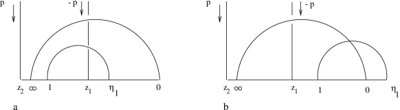
Figure 9: String worldsheets corresponds to field theory diagrams Fig. 4e, 6a and 4b.

Since there is no intersection between the two loops, the only modification is in $B_{I}$. We have

$${(-A^{0}/2)^{-1}}=\frac{1}{\Delta}\left(\begin{array}[]{cc}(t_{1}+t_{3}){\bf 1}&-t_{3}{\bf 1}\cr-t_{3}{\bf 1}&(t_{2}+t_{3}){\bf 1}\end{array}\right).$$ (4.29)

and

$$B_{I}^{\mu}={B^{0}}^{\mu}_{I}+\frac{i}{2}(\theta p)^{\mu}\left(\begin{array}[]{c}1\cr 1\end{array}\right).$$ (4.30)

Thus, after the integration over the momenta running in the loops, the string formula gives the following $\theta$ dependent part

$$-\frac{1}{2}B^{T}A^{-1}B=\frac{(t_{1}+t_{3})\alpha_{2}^{2}+(t_{2}+t_{3})\alpha_{1}^{2}+2\alpha_{1}\alpha_{2}t_{3}}{\Delta}p^{2}-\frac{1}{4\Delta}(\theta p)^{2}(t_{1}+t_{2}).$$ (4.31)

Together with measure factor $\Delta^{-d/2}$ and the other pieces coming from $\tilde{V}_{N;h}^{0}$ and $C_{0}$, the $\theta$ independent piece of (3.22) is exactly the same as the field theory integrand (4.10). Moreover, the $\theta$-dependence is also precisely reproduced.

A remark about the integration region is in order. As explained in [120], the corner of $z_{i}$’s considered yields the correct functional form of Feynman diagram in Fig. 4e, but does not reproduce the field theory integration region over the Schwinger parameters. However, we know that a field theory diagram is identified with the sum of contributions from a few different corners of the string moduli space. This sum reconstructs the expected field theory integration region, without modifying the integrand previously found. Since turning on a $B$-field does not change this identification, the situation is therefore the same as in [120]. It is easy to check that the complete field theory result (4.10) is reproduced from string theory.

Next we consider the string worldsheet configuration of Fig 9 b. In this case,

$$-A/2=\left(\begin{array}[]{cc}(t_{1}+t_{3}){\bf 1}&t_{3}{\bf 1}+\frac{i}{2}\theta\cr t_{3}{\bf 1}-\frac{i}{2}\theta&(t_{2}+t_{3}){\bf 1}\end{array}\right),$$ (4.32)

where again we have written $A$ as a $2\times 2$ block with ${\bf 1}$ and $\theta$ being $d\times d$ matrices. It is easy to work out the inverse,

$$(-A/2)^{-1}=\frac{1}{\Delta_{\theta}}\left(\begin{array}[]{cc}(t_{2}+t_{3}){\bf 1}&-t_{3}{\bf 1}-\frac{i}{2}\theta\cr-t_{3}{\bf 1}+\frac{i}{2}\theta&(t_{1}+t_{3}){\bf 1}\end{array}\right).$$ (4.33)

As for $B$, it is

$$\frac{1}{2}\left(\begin{array}[]{c}B_{1}^{\mu}\cr B_{2}^{\mu}\end{array}\right)=\left(\begin{array}[]{c}\alpha_{1}p^{\mu}+\frac{i}{2}(\theta p)^{\mu}\cr-\alpha_{2}p^{\mu}\end{array}\right).$$ (4.34)

Therefore

$$-\frac{1}{2}B^{T}A^{-1}B=p\frac{(t_{1}+t_{3})\alpha_{2}^{2}+(t_{2}+t_{3})\alpha_{1}^{2}+2\alpha_{1}\alpha_{2}t_{3}}{{\Delta_{\theta}}}p+(t_{2}+t_{3}-2\alpha_{2})p\frac{\theta^{2}}{4{\Delta_{\theta}}}p.$$ (4.35)

Again the complete field theory result (4.17) including the region of integration is reproduced.

Finally we consider the field theory diagram Fig. 6a. As explained in [119], Fig. 9a actually contributes to both types of field theory diagrams: Fig. 4e with external legs in distinct propagators and Fig. 6a with external legs on the same propagator. One has to be careful in selecting the range of the punctures in order to get the desired correspondence. For the present case of Fig. 6a, one has to consider the range $z_{2}\in[-1,-\eta]$ and $(z_{1}-\eta)/(z_{1}-1)\in[-1,-\eta]$. According to (3.12)-(3.14), $A$ is unmodified from $A_{0}$ and is given by (4.27) since there is no intersection of the loops. As for $B$, it is given by (4.30). The only difference from the case of Fig. 4e is in the range of the punctures $z_{1},z_{2}$ and hence a different expression of $B^{0}$

$$\frac{1}{2}\left(\begin{array}[]{c}{B^{0}}_{1}^{\mu}\cr{B^{0}}_{2}^{\mu}\end{array}\right)=\left(\begin{array}[]{c}\alpha_{2}p^{\mu}\cr\alpha_{2}p^{\mu}\end{array}\right)~{}.$$ (4.36)

For our purpose, we concentrate on the $\theta$ independent terms. Precisely the $\theta^{2}$ term in (4.21) is reproduced and confirm the complete field theory result.

We have also checked the other field theory diagrams in Fig 4 and 6 and they are all reproduced correctly from the string master formula (3.22).

5 Conclusions and Discussions

In this paper, we used the open string operator formalism to construct multiloop string amplitudes with $B$-field. The key observation is that when expressed in terms of the commutation relations of the string modes, the effects of noncommutativity is very simple: apart from an overall scaling of the operators, only the zero mode commutation relation is modified. This allowed us to repeat the basic steps in operator formalism and construct multiloop string amplitudes with $B$-fields. In particular, we constructed the open string vertex operators and determined directly the one-loop open string Green function. For higher loop amplitudes, we constructed the multiloop Reggeon vertex by sewing together legs of a tree level Reggeon vertex. It was thus possible to write down explicitly string amplitudes with $B$-field with any number of loops. Moreover one-one correspondence between corners of open string moduli space and Feynman diagrams is again established.

With the master formula at our disposal, it is in principle possible to tackle many field theory questions, which may appear mysterious otherwise, from the string point of view. This is one major advantage of the string approach. One such question is the UV/IR effect in noncommutative field theory. Since the $\theta$ dependences in any higher loop amplitude are isolated explicitly in our master formula (3.22), by taking the field theory limit of the string result, one can do a systematic analysis of the UV/IR effects in a noncommutative field theory at arbitrary loop levels. Thus this approach may provide an uniform string theory understanding of the UV/IR effect.

Another possible application is in the understanding of a similar effect in 3-dimension. It was found in [79] that a Majorana fermion induces a noncommutative Chern-Simons action at one loop. The coefficient is a step function which is $1/2$ when the theory is noncommutative and is 0 when the theory is commutative. It would be interesting to understand this as well as other perturbative aspects of this theory from the string point of view.

Although we did not write down explicitly the open string Green function for higher loop, it is easy to extract it from the master formula (3.22). It is also easy to generalize the considerations of this paper to the superstring case and to put Chan-Paton factors to obtain results for noncommutative field theory with $U(N)$ gauge group.

So far, noncommutative D-branes appear in string theory in two basic forms: Moyal-deformation in the case of flat spacetime with $B$-field, and “fuzzy deformation” in the case of D-branes in WZW model. In particular the latter is generically a more general nonassociative deformation [93]. It would be interesting to explore other possibility of noncommutative geometry and deformation that can arise in string and M-theory.

We hope to return to some of these issues in the future.

Acknowledgments

This work was partially supported by the Swiss National Science Foundation, by the European Union under TMR contract ERBFMRX-CT96-0045, by the Swiss Office for Education and Science and by MURST (Italy).

References

- [1] M. R. Douglas, C. Hull, D-Branes and the Non-Commutative Torus, J. High Energy Phys. 2 (1998) 8, hep-th/9711165.
- [2]
- [3] A. Connes, M. R. Douglas, A. Schwarz, Noncommutative Geometry and Matrix Theory: Compactification on Tori, J. High Energy Phys. 02 (1998) 003, hep-th/9711162.
- [4]
- [5] A. Connes, Noncommutative Geometry, Academic Press (1994).
- [6] G. Landi, An Introduction to Noncommutative Spaces and their Geometries, Springer-Verlag (1997).
- [7] J. Madore, An Introduction to Noncommutative Differential Geometry and its Physical Applications, Cambridge University Press (1999).
- [8]
- [9] Y.-K. E. Cheung, M. Krogh, Noncommutative Geometry From 0-Branes in a Background Field, Nucl. Phys. B528 (1998) 185, hep-th/9803031;
- [10] T. Kawano, K. Okuyama, Matrix Theory on Noncommutative Torus, Phys. Lett. B433 (1998) 29, hep-th/9803044;
- [11] F. Ardalan, H. Arfaei, M. M. Sheikh-Jabbari, Noncommutative Geometry from Strings and Branes, JHEP 9902 (1999) 016, hep-th/9810072.
- [12]
- [13] C.-S. Chu, P.-M. Ho, Noncommutative Open String and D-brane, Nucl. Phys. B550 (1999) 151, hep-th/9812219;
- [14] C.-S. Chu, P.-M. Ho, Constrained Quantization of Open String in Background B Field and Noncommutative D-brane, Nucl. Phys., B568 (2000) 447, hep-th/9906192.
- [15]
- [16] V. Schomerus, D-Branes and Deformation Quantization, JHEP 9906 (1999) 030, hep-th/9903205.
- [17]
- [18] N. Seiberg, E. Witten, String Theory and Noncommutative Geometry, JHEP 9909 (1999) 032, hep-th/9908142.
- [19]
- [20] C.-S. Chu, P.-M. Ho, M. Li, Matrix Theory in a Constant C Field Background, Nucl. Phys., in press, hep-th/9911153.
- [21]
- [22] A. Abouelsaood, C.G. Callan, C.R. Nappi, S.A. Yost, Open Strings in Background Gauge Fields, Nucl. Phys. B280 (1987) 599;
- [23] C.-S. Chu, Noncommutative Open String: Neutral and Charged, hep-th/0001144.
- [24]
- [25] T. Filk, Divergences in a Field Theory on Quantum Space, Phys.Lett. B376 (1996)53.
- [26]
- [27] S. Minwalla, M.V. Raamsdonk, N. Seiberg, Noncommutative Perturbative Dynamics, hep-th/9912072.
- [28]
- [29] M.V. Raamsdonk, N. Seiberg, Comments on Noncommutative Perturbative Dynamics, hep-th/0002186.
- [30]
- [31] J.C. Varilly, J.M. Gracia-Bondia, On the ultraviolet behavior of quantum fields over noncommutative manifolds, Int. J. Mod. Phys. A14 (1999) 1305, hep-th/9804001.
- [32]
- [33] M. Chaichian, A. Demichev, P. Presnajder, Quantum Field Theory on Noncommutative Space-times and the Persistence of Ultraviolet Divergences, hep-th/9812180.
- [34]
- [35] C.P. Martin, D. Sanchez-Ruiz, The One-loop UV Divergent Structure of U(1) Yang-Mills Theory on Noncommutative , hep-th/9903077.
- [36] M. Sheikh-Jabbari, One Loop Renormalizability of Supersymmetric Yang-Mills Theories on Noncommutative Torus, JHEP 06 (1999) 015, hep-th/9903107.
- [37] T. Krajewski, R. Wulkenhaar, Perturbative quantum gauge fields on the noncommutative torus, hep-th/9903187.
- [38]
- [39] D. Bigatti, L. Susskind, Magnetic fields, branes and noncommutative geometry, hep-th/9908056.
- [40]
- [41] Z. Yin, A Note On Space Noncommutativity, hep-th/9908152.
- [42]
- [43] M. Li, Strings from IIB Matrices , Nucl. Phys. B499 (1997) 149, hep-th/9612222;
- [44] H. Aoki, N. Ishibashi, S. Iso, H. Kawai, Y. Kitazawa, T. Tada, Noncommutative Yang-Mills in IIB Matrix Model, hep-th/9908141;
- [45]
- [46] N. Ishibashi, S. Iso, H. Kawai, Y. Kitazawa, Wilson Loops in Noncommutative Yang Mills, hep-th/9910004.
- [47]
- [48] S. Iso, H. Kawai, Y. Kitazawa, Bi-local Fields in Noncommutative Field Theory, hep-th/0001027.
- [49]
- [50] O. Andreev, A Note on Open Strings in the Presence of Constant B-Field, hep-th/0001118.
- [51]
- [52] H. Grosse, T. Krajewski, R. Wullkenhaar, Renormalization of noncommutative Yang-Mills theories: A simple example, hep-th/0001182.
- [53]
- [54] J. Madore, S. Schraml, P. Schupp, J. Wess, Gauge Theory on Noncommutative Spaces, hep-th/0001203.
- [55]
- [56] I. Bars, D. Minic, Non-Commutative Geometry on a Discrete Periodic Lattice and Gauge Theory, hep-th/9910091;
- [57] J. Ambjorn, Y. M. Makeenko, J. Nishimura, R. J. Szabo, Nonperturbative Dynamics of Noncommutative Gauge Theory, hep-th/0002158.
- [58]
- [59] I. Chepelev, R. Roiban, Renormalization of Quantum Field Theories on Noncommutative , I. Scalars, hep-th/9911098.
- [60]
- [61] I. Ya. Aref’eva, D. M. Belov, A. S. Koshelev, Two-Loop Diagrams in Noncommutative theory, hep-th/9912075; A Note on UV/IR for Noncommutative Complex Scalar Field, hep-th/0001215.
- [62]
- [63] M. Hayakawa, Perturbative analysis on infrared aspects of noncommutative QED on , hep-th/9912094; Perturbative analysis on infrared and ultraviolet aspects of noncommutative QED on , hep-th/9912167.
- [64]
- [65] A. Matusis, L. Susskind, N. Toumbas, The IR/UV Connection in the Non-Commutative Gauge Theories, hep-th/0002075.
- [66]
- [67] C.-S. Chu, F. Zamora, Manifest Supersymmetry in Non-Commutative Geometry, JHEP 02 (2000) 022, hep-th/9912153;
- [68] A. Schwarz, Noncommutative supergeometry and duality, hep-th/9912212;
- [69] S. Ferrara, M. A. Lledo, Some Aspects of Deformations of Supersymmetric Field Theories, hep-th/0002084;
- [70] S. Terashima, A Note on Superfields and Noncommutative Geometry, hep-th/0002119.
- [71]
- [72] W. Fischler, J. Gomis, E. Gorbatov, A. Kashani-Poor, S. Paban, P. Pouliot, Evidence for Winding States in Noncommutative Quantum Field Theory, hep-th/0002067;
- [73] G. Arcioni, J. L. F. Barbon, Joaquim Gomis, M. A. Vazquez-Mozo, On the stringy nature of winding modes in noncommutative thermal field theories, hep-th/0004080.
- [74]
- [75] F. Ardalan, N. Sadooghi, Axial Anomaly in Non-Commutative QED on , hep-th/0002143;
- [76] J. M. Gracia-Bondia, C. P. Martin, Chiral Gauge Anomalies on Noncommutative , hep-th/0002171;
- [77] L. Bonora, M. Schnabl, A. Tomasiello, A note on consistent anomalies in noncommutative YM theories, hep-th/0002210.
- [78]
- [79] C.-S. Chu, Induced Chern-Simons and WZW action in Noncommutative Spacetime, Nucl. Phys. in press, hep-th/0003007.
- [80]
- [81] R. Blumenhagen, L. Goerlich, B. Kors, D. Lust, Asymmetric Orbifolds, Noncommutative Geometry and Type I String Vacua, hep-th/0003024.
- [82]
- [83] R. Gopakumar, S. Minwalla, A. Strominger, Noncommutative Solitons, hep-th/0003160.
- [84]
- [85] N. Ishibashi, S. Iso, H. Kawai, Y. Kitazawa, String Scale in Noncommutative Yang-Mills, hep-th/0004038.
- [86]
- [87] F. Zamora, On the Operator Product Expansion in Noncommutative Quantum Field Theory, hep-th/0004085.
- [88]
- [89] A. Rajaraman, M. Rozali, Noncommutative Gauge Theory, Divergences and Closed Strings, hep-th/0003227.
- [90]
- [91] J. Gomis, K. Landsteiner, E. Lopez, Non-Relativistic Non-Commutative Field Theory and UV/IR Mixing, hep-th/0004115.
- [92]
- [93] A. Yu. Alekseev, A. Recknagel, V. Schomerus, Non-commutative World-volume Geometries: Branes on SU(2) and Fuzzy Spheres, JHEP 9909 (1999) 023, hep-th/9908040.
- [94]
- [95] A. Yu. Alekseev, A. Recknagel, V. Schomerus, Brane Dynamics in Background Fluxes and Non-commutative Geometry, hep-th/0003187;
- [96] C. Bachas, M. Douglas, C. Schweigert, Flux Stabilization of D-branes, hep-th/0003037;
- [97] J. Pawelczyk, SU(2) WZW D-branes and their non-commutative geometry from DBI action, hep-th/0003057.
- [98]
- [99] O. Andreev, H. Dorn, Diagrams of Noncommutative Phi-Three Theory from String Theory, hep-th/0003113.
- [100]
- [101] Y. Kiem, S. Lee, UV/IR Mixing in Noncommutative Field Theory via Open String Loops, hep-th/0003145.
- [102]
- [103] A. Bilal, C.-S. Chu, R. Russo, String Theory and Noncommutative Field Theories at One Loop, hep-th/0003180.
- [104]
- [105] J. Gomis, M. Kleban, T. Mehen, M. Rangamani, S. Shenker, Noncommutative Gauge Dynamics From The String Worldsheet, hep-th/0003215.
- [106]
- [107] H. Liu, J. Michelson, Stretched Strings in Noncommutative Field Theory, hep-th/0004013.
- [108]
- [109] S. Sciuto, The general vertex function in Dual Resonance Models, Lettere al Nuovo Cimento 2(1969), 411;
- [110] A. Della Selva and S. Saito, A simple expression for the Sciuto three-reggeon vertex generating duality, Lettere al Nuovo Cimento 4(1970), 689.
- [111]
- [112] P. Di Vecchia, R. Nakayama, J.L. Petersen, S. Sciuto, Properties of the three-Reggeon vertex in string theories, Nucl. Phys. 282 (1987) 103.
-
[113]
A. Neveu and P. West,
“Symmetries Of The Interacting Gauge Covariant Bosonic String,”
Nucl. Phys. B278 (1986) 601;
A. Neveu and P. West, “Group Theoretic Approach To The Perturbative String S Matrix,” Phys. Lett. B193 (1987) 187. - [114] P. Di Vecchia, M. Frau, A. Lerda, S. Sciuto, A Simple Expression for the MultiLoop Amplitude in the Bosonic String, Phys. Lett. B199 (1987) 49.
- [115] P. Di Vecchia, M. Frau, A. Lerda, S. Sciuto, -String Vertex and Loop Calculation in the Bosonic String, Nucl. Phys. B298 (1988) 526.
- [116] C. Lovelace, Simple N-Reggeon vertex, Phys. Lett. B32 (1970) 490.
- [117] P. Di Vecchia, F. Pezzella, M. Frau, K. Hornfeck, A. Lerda, S. Sciuto, -point -loop vertex for a free bosonic theory with vacuum charge , Nucl. Phys. B322 (1989) 317.
- [118] P. Di Vecchia, A. Lerda, L. Magnea, R. Marotta, R. Russo, String techniques for the calculation of renormalization constants in field theory, Nucl. Phys. B469 (1996) 235, hep-th/9601143.
-
[119]
P. Di Vecchia, A. Lerda, L. Magnea, R. Marotta, R. Russo,
Two-loop scalar diagrams from string theory , hep-th/9607141;
R. Marotta, F. Pezzella, Two-Loop -Diagrams from String Theory, Phys. Rev. D61 (2000) 106006, hep-th/9912158; String-generated quartic scalar interactions, hep-th/0003044. - [120] Alberto Frizzo, Lorenzo Magnea, Rodolfo Russo, Scalar field theory limits of bosonic string amplitudes, hep-th/9912183.