Constructing the light-front QCD Hamiltonian

 

We propose the light-front Lagrangian and the corresponding Hamiltonian that produce a theory perturbatively equivalent to the conventional QCD in the Lorentz coordinates after the regularization is removed. The regularization used is nonstandard and breaks the gauge invariance. But after the regularization is removed, this invariance is restored by the introduction of a finite number of counterterms with coefficients dependent on the regularization parameters.

In this corrected version the counterterms are given in more exact form.

Original version is published in Theoretical and Mathematical Physics,
Vol. 120, No. 3, pp. 1164-1181, 1999;

translated from Teoreticheskaya i Maternaticheskaya Fizika,
Vol. 120, No. 3, pp. 417-437, September, 1999.

1.  Introduction

The search for ways to solve problems in the quantum field theory with a large coupling constant, has long been significant. Calculations on space-time lattices are now often used for this purpose in QCD. Essential results have been thus obtained. Nevertheless, these calculations are very laborious and have a low accuracy; in addition, it is generally difficult to estimate the calculation error theoretically. Therefore, it is interesting to seek other possible approaches to this problem. Even limited progress in this direction would allow comparing the results obtained by different methods.

Long before the advent of QCD, studying the pion-nucleon interaction had been attempted by solving the Schrodinger equation in the Lorentz coordinate system in the framework of the quantum theory of pion and nucleon fields. The states were described by the method previously found by V. A. Fock [1] in terms of vectors in the space that now bears his name. In this case, the mathematical vacuum of the Fock space coincided with the free theory vacuum. This approach, now known as the Tamm-Dancoff method [2, 3], did not lead to success. The primary reason was the complexity of the physical vacuum state, which did not coincide with the mathematical vacuum. Without a description of the physical vacuum, it was impossible to investigate any other states. If ultraviolet (UV) and infrared (IR) cutoffs are introduced to make the number of degrees of freedom finite, it would be possible, in principle, to represent the physical vacuum as a vector of the Fock space with the free theory vacuum. However, such a representation proves extremely complicated because it is necessary to provide the translation invariance of the physical vacuum and to satisfy the ”cluster decomposition property” for vacuum expectation values. For these reasons, the Schrodinger equation in the Lorentz coordinates, where the evolution occurs in the conventional time, is hardly applicable to any calculations in the quantum field theory with a large coupling constant.

As early as 1949, Dirac suggested a method for avoiding the difficulties related to the description of the physical vacuum state [4]. He proposed using the light-front coordinates $x^{\pm}=(x^{0}\pm x^{3})/\sqrt{2}$, $x^{1}$, $x^{2}$, where $x^{0}$, $x^{1}$, $x^{2}$, $x^{3}$ are the Lorentz coordinates, and treating $x^{+}$ as time. In this approach, a theory is canonically quantized on the surface $x^{+}=const$, and the generator $P_{+}$ of the shift along the $x^{+}$ axis plays the role of the Hamiltonian $H$. In addition, the generator of the shift along the $x^{-}$ axis, i.e., the momentum operator $P_{-}$, does not shift the surface $x^{+}=const$, where the quantization is performed, and is kinematic, according to the Dirac terminology (in contrast to the dynamic generator $P_{+}$). Therefore, the structure of the operator $P_{-}$ in a theory with interaction is the same as in a theory without interaction, i.e., the operator $P_{-}$ is always quadratic in the creation and annihilation operators ${a_{n}}^{+}(p_{-},p_{\bot})$ and $a_{n}(p_{-},p_{\bot})$ and, as a rule, has the form (after normal ordering)

$$\halign{\hbox to\displaywidth{$\hfil\displaystyle#\hfil$}\cr 0.0pt{\hfil$\displaystyle P_{-}=\int d^{2}p_{\bot}\int\limits_{0}^{\infty}dp_{-}\;p_{-}\sum_{n}{a_{n}}^{+}(p_{-},p_{\bot})a_{n}(p_{-},p_{\bot}),\crcr}}$$

where $p_{\bot}=(p_{1},p_{2})$ and the index $n$ enumerates the species of the creation and annihilation operators. According to the spectral condition, the operator $P_{-}$ is positive definite; therefore, the integration over $p_{-}$ in the given formula is performed only from $0$ to $\infty$. The operator $P_{-}$ vanishes on the physical vacuum $\Omega$, i.e., $P_{-}|\Omega\rangle=0$, whence it follows that $a_{n}(p_{-},p_{\bot})|\Omega\rangle=0$.

For this reason, the physical vacuum $|\Omega\rangle$ can be taken as the mathematical vacuum of the Fock space generated by the operators ${a_{n}}^{+}$. No question of describing the physical vacuum structure arises. The spectrum of the bound states can be found by solving the Schrodinger equation

$$\halign{\hbox to\displaywidth{$\hfil\displaystyle#\hfil$}\cr 0.0pt{\hfil$\displaystyle P_{+}|\Psi\rangle=p^{\prime}_{+}|\Psi\rangle\crcr}}$$

under the conditions

$$\halign{\hbox to\displaywidth{$\hfil\displaystyle#\hfil$}\cr 0.0pt{\hfil$\displaystyle P_{-}|\Psi\rangle=p^{\prime}_{-}|\Psi\rangle,\quad P_{\bot}|\Psi\rangle=0,\crcr}}$$

where $p^{\prime}_{+}$, $p^{\prime}_{-}$ are numbers and the mass squared is defined by

$$\halign{\hbox to\displaywidth{$\hfil\displaystyle#\hfil$}\cr 0.0pt{\hfil$\displaystyle m^{2}=2p^{\prime}_{+}p^{\prime}_{-}.\crcr}}$$

Here, $|\Psi\rangle$ is a vector in the just mentioned Fock space. It is easy to satisfy the conditions $P_{-}|\Psi\rangle=p^{\prime}_{-}|\Psi\rangle$ and $P_{\bot}|\Psi\rangle=0$, where $p^{\prime}_{-}$ is chosen arbitrarily. The problem is to solve the Schrodinger equation. Such an approach is usually called the ”light-front Hamiltonian” approach. Obviously, it can also be used to calculate the scattering matrix.

The scheme described faces considerable problems due to divergences that arise and the lack of the explicit Lorentz invariance. But the possibility of avoiding the direct description of the physical vacuum structure is such a considerable advantage that this approach continues to attract attention. Interest in it has increased with the advent of QCD. This paper is devoted to developing this approach.

We note that the light-front coordinates and the similar ”infinitely large-momentum system” are used in quantum field theory not only in the framework of the Hamiltonian approach based on directly solving the Schrodinger equation. Many results have been obtained by studying the limiting case of fast-moving reference frames in the framework of the explicitly Lorentz-invariant. theory of the scattering matrix or of the Green’s functions [5, 6, 7, 8, 9]. But we consider only the Hamiltonian approach in this paper.

For the theory with the given Lorentz-invariant initial action, constructing the light-front Hamiltonian $P_{+}$ proves a difficult problem. The primary reason is the specific divergences at zero values of tin’ momentum $p_{-}$ of virtual quanta. In particular, the invariant volume element on the hyperboloid $p_{\mu}p^{\mu}=m^{2}$ has the form $d^{2}p_{\bot}dp_{-}/p_{-}$ and contains $p_{-}$ in the denominator. The situation becomes more complicated in gauge theories. Even in the first papers on this problem [10, 11], it became clear that canonical quantization on the surface $x^{+}=const$ could be performed only in the gauge $A_{-}=0$ or in similar gauges (for example, $\partial_{-}A_{-}=0$). The reason is that second-class constraints arise in the theory and solving them, in particular, requires inverting the covariant derivative $D_{-}=\partial_{-}+igA_{-}$. But in the gauge $A_{-}=0$, the Feynman propagator has an extra term $p_{-}$ in the denominator, which strengthens the singularities at $p_{-}=0$ (at least, in the perturbation theory).

As a consequence, a special regularization is required, which consists in ”cutting out” the neighborhood of $p_{-}=0$ in the momentum space one way or another and which results in breaking the Lorentz invariance (until the regularization is removed). This is unavoidable in the liglit-front Hamiltonian approach. In principle, we can preserve the gauge invariance if, instead of ”cutting out” the neighborhood of $p_{-}=0$, we restrict the space-time with respect to the coordinate $x^{-}$ ($-L\leq x^{-}\leq L$) and impose periodic boundary conditions in $x^{-}$ on all fields [12]. In this case, the spectrum of the momentum $P_{-}$ becomes discrete, and the ”zero modes” of the fields $A$, i.e., the Fourier modes corresponding to $p_{-}=0$, are explicitly singled out. To preserve the gauge invariance, these zero modes must be taken into account. It was shown in [12] that secondary second-class constraints arise in the theory, from which we must find the above-mentioned zero modes as functions of the other modes and substitute them in the Hamiltonian. These constraints arc so complicated that solving them proves impossible. Therefore, from the very beginning, we must discard the zero modes in the Lagrangian, which results in breaking the gauge invariance. Therefore, the breakdown of the gauge invariance by a regularization is unavoidable in any case. In what follows, to regularize the theory, we ”cut out” the neighborhood of $p_{-}=0$. In addition, the conventional UV regularization is, of course, necessary.

It follows from the above discussion that the formal canonical quantization on the hypersurface $x^{+}=const$ can produce a Hamiltonian corresponding to a theory that is not equivalent to the initial Lorentz-invariant one, even in the limit of removing the regularization. As a rule, the equivalence can be provided only by adding nonconventional counterterms [13, 14, 15] to the light-front Hamiltonian.

In the last few years, a number of papers have appeared in which the approximate regularized light-front QCD Hamiltonian was directly constructed [16, 17]. Using the renormalization group theory, the form of the Hamiltonian was adjusted based on the requirement that the result be weakly dependent on the UV cutoff, with the relation to the conventional Lorentz-invariant theory not being traced in detail. Methods for simplifying the Hamiltonian and solving the Schrodinger equation were also proposed. The technique described in these papers is of considerable interest and continues to develop. But it remains unclear to what extent the light-front theory thus obtained corresponds to the conventional Lorentz-invariant QCD.

In this connection, we meet the problem of constructing the light-front Hamiltonian such that it produces a theory equivalent to the conventional Lorentz-invariant one in the limit of removing the regularization. As a necessary condition, we should first provide this equivalence in the framework of the perturbation theory. Then, in particular, we can use the technique described in [16, 17] to simplify the obtained Hamiltonian and the subsequent nonperturbative calculations based on the Schrodinger equation. In doing so, we see the relation to the conventional Lorentz-invariant theory.

The problem of constructing the counterterms for the light-front Hamiltonian, which provide the equivalence of this approach to the Lorentz-invariant one, was investigated in [13] in the framework of the perturbation theory in the coupling constant. In that paper, the authors proposed a method for comparing two perturbation series for the Green’s functions constructed using the light-front Hamiltonian for one and the conventional Lorentz-invariant approach for the other. In addition to the UV regularization, they regularized the singularities at $p_{-}=0$ using the cutoff $|p_{-}|\geq\varepsilon>0$, i.e., eliminating the Fourier components with $|p_{-}|<\varepsilon$ for every field in the theory. It was revealed that for the required equivalence for the nongauge field theories (in particular, for the Yukawa model), it was only necessary to add a few counterterms to the canonical light-front Hamiltonian. But for gauge theories (both Abelian and non-Abelian) under the given regularization, it proved necessary to introduce an infinite number of counterterms in the Hamiltonian. This situation is closely related to the gauge condition $A_{-}=0$, which is unavoidable in the canonical light-front quantization. It is known [18, 19] that to correctly construct the perturbation theory in this gauge, it is necessary to use the gauge field propagator in the form proposed by Mandelstam and Leibbrandt [20, 21]

$$\halign{\hbox to\displaywidth{$\hfil\displaystyle#\hfil$}\cr 0.0pt{\hfil$\displaystyle\hfill\frac{-i\delta^{ab}}{k^{2}+i0}\left(g_{\mu\nu}-\frac{k_{\mu}n_{\nu}+k_{\nu}n_{\mu}}{2k_{+}k_{-}+i0}2\frac{k_{+}}{n_{+}}\right)=\frac{-i\delta^{ab}}{k^{2}+i0}\left(g_{\mu\nu}-\frac{k_{\mu}n_{\nu}+k_{\nu}n_{\mu}}{2(kn^{*})(kn)/(nn^{*})+i0}2\frac{(kn^{*})}{(nn^{*})}\right)\hfill(1)\cr}}$$

where $\mu,\nu=+,-,1,2$; $k_{\pm}=(k_{0}\pm k_{3})/\sqrt{2}$; $n_{-,1,2}=0$, $n^{*}_{+,1,2}=0$. The additional pole in $k_{-}$ in this expression is cut out with the regularization $|k_{-}|\geq\varepsilon$. The distortion arising in this case does not disappear in the limit $\varepsilon\to 0$. An infinite number of counterterms is required to compensate this distortion.

The aim of this paper is to overcome this difficulty and obtain the required Hamiltonian with a finite number of counterterms. In such a case, we must change the regularization. For this purpose, we propose shifting the pole with respect to $k_{-}$ in expression (1.  Introduction) from the point $k_{-}=0$ by changing the Lagrangian such that a small regularizing mass parameter $\mu^{2}$ is added to the quantity $2k_{+}k_{-}$. In this case, the distortions caused by cutting out the interval $|k_{-}|<\varepsilon$ are not so large as in the preceding case, and a finite number of counterterms is sufficient to obtain the correct Hamiltonian in the limit of removing the regularization ($\varepsilon\to 0$ and then $\mu\to 0$ together with $\Lambda\to\infty$, where $\Lambda$ is a UV regularization parameter). We choose the UV regularization such that, after removing the IR regularization (i.e., after setting $\varepsilon=0$ and $\mu=0$) at the intermediate stages, we obtain the Lorentz-invariant Lagrangian regularized in the UV region. This increases the number of ”ghosts,” but the number of necessary counterterms would otherwise increase sharply. We note that in the gauge $A_{-}=0$, the one-particle irreducible vertex parts with the upper index ”$-$” do not contribute to the Green’s functions. In what follows, we prove the coincidence of every order of the perturbation theory in the limit of removing the regularization only for the Green’s functions and not for the vertex parts with the index ”$-$”. This is sufficient because the masses of the bound states are determined by the poles of the Green’s functions.

Under the given regularization, the Hamiltonian acts on the space with an indefinite metric, which prevents using the conventional variational principle to solve the Schrodinger equation under the conditions of preserving the regularization. Nevertheless, there exist different variational methods that allow solving this equation.

The chosen regularization breaks the local gauge invariance but preserves the global $SU(3)$ invariance. For this reason, the number of necessary counterterms, being finite, is essentially larger than the conventional one. We show that there is a way to choose the counterterms such that the obtained light-front theory is perturbatively equivalent to the initial Lorentz-invariant one in the limit of removing the regularization.

We achieve this goal by starting with the Lagrangian

$$\halign{\hbox to\displaywidth{$\hfil\displaystyle#\hfil$}\cr 0.0pt{\hfil$\displaystyle\hfill L=L_{0}+L_{I}\hfill(2)\cr}}$$

$$\halign{\hbox to\displaywidth{$\hfil\displaystyle#\hfil$}\cr 0.0pt{\hfil$\displaystyle\hfill L_{0}=-\frac{1}{4}\sum_{j=0,1}(-1)^{j}f_{j}^{a,\mu\nu}\left(1+\frac{\partial_{\scriptscriptstyle\|}^{2}}{\Lambda^{2}_{j}}-\frac{\partial_{\bot}^{2}}{\Lambda^{2}}\right)f_{j,\mu\nu}^{a}+\hfill\phantom{(3)}\cr 0.0pt{\hfil$\displaystyle\hfill+\sum_{l=0}^{3}\frac{1}{v_{l}}\bar{\psi}_{l}\left(i\gamma^{\mu}\partial_{\mu}-M_{l}\right)\psi_{l}\hfill(3)\cr}}}$$

$$\halign{\hbox to\displaywidth{$\hfil\displaystyle#\hfil$}\cr 0.0pt{\hfil$\displaystyle\hfill L_{I}=c_{0}\partial_{\mu}A^{a}_{\nu}\partial^{\mu}A^{a,\nu}+c_{01}\partial_{\mu}A^{a}_{\nu}\,N^{\mu\alpha}\,\partial_{\alpha}A^{a,\nu}+c_{1}\partial_{\mu}A^{a,\mu}\,\partial_{\nu}A^{a,\nu}+c_{11}\,N^{\mu\alpha}\,\partial_{\mu}A^{a}_{\alpha}\,\partial_{\nu}A^{a,\nu}+\hfill\phantom{(4)}\cr 0.0pt{\hfil$\displaystyle\hfill+c_{12}\,N^{\mu\alpha}\,\partial_{\mu}A^{a}_{\alpha}\,N^{\nu\beta}\,\partial_{\nu}A^{a}_{\beta}+c_{2}A^{a}_{\mu}A^{a,\mu}+c_{3}f^{abc}A^{a}_{\mu}A^{b}_{\nu}\partial^{\mu}A^{c,\nu}+c_{31}f^{abc}A^{a}_{\mu}A^{b}_{\nu}\,N^{\alpha\mu}\,\partial_{\alpha}A^{c,\nu}+\hfill\phantom{(4)}\cr 0.0pt{\hfil$\displaystyle\hfill+A^{a}_{\mu}A^{b}_{\nu}A^{c}_{\gamma}A^{d}_{\delta}\bigl{(}c_{4}f^{abe}f^{cde}g^{\mu\gamma}g^{\nu\delta}+\delta^{ab}\delta^{cd}\left(c_{5}g^{\mu\gamma}g^{\nu\delta}+c_{6}g^{\mu\nu}g^{\gamma\delta}\bigr{)}\right)+\hfill\phantom{(4)}\cr 0.0pt{\hfil$\displaystyle\hfill+c_{7}\bar{\psi}\gamma^{\mu}i\partial_{\mu}\psi+c_{71}\bar{\psi}\gamma_{\mu}\,N^{\mu\nu}\,i\partial_{\nu}\psi+c_{72}\bar{\psi}\gamma_{\mu}\,N^{\nu\mu}\,i\partial_{\nu}\psi-c_{8}\bar{\psi}\psi+\hfill\phantom{(4)}\cr 0.0pt{\hfil$\displaystyle\hfill+c_{9}A^{a}_{\mu}\bar{\psi}\gamma^{\mu}\frac{\lambda^{a}}{2}\psi+c_{91}A^{a}_{\alpha}\,N^{\mu\alpha}\,\bar{\psi}\gamma_{\mu}\frac{\lambda^{a}}{2}\psi,\hfill(4)\cr}}}}}}$$

where

$$\halign{\hbox to\displaywidth{$\hfil\displaystyle#\hfil$}\cr 0.0pt{\hfil$\displaystyle\hfill f^{a}_{j,\mu\nu}=\partial_{\mu}A^{a}_{j,\nu}-\partial_{\nu}A^{a}_{j,\mu},\qquad\frac{1}{\Lambda_{j}^{2}}=\cases{1/\Lambda^{2},&$j=0$,\cr 1/\Lambda^{2}+1/\mu^{2},&$j=1$,\cr}\hfill(5)\cr}}$$

$$\halign{\hbox to\displaywidth{$\hfil\displaystyle#\hfil$}\cr 0.0pt{\hfil$\displaystyle\hfill v_{0}=1,\quad\sum_{l=0}^{3}v_{l}=0,\quad\sum_{l=0}^{3}v_{l}M_{l}=0,\quad\sum_{l=0}^{3}v_{l}M_{l}^{2}=0,\hfill(6)\cr}}$$

$$\halign{\hbox to\displaywidth{$\hfil\displaystyle#\hfil$}\cr 0.0pt{\hfil$\displaystyle\hfill A^{a}_{\mu}=\sum_{j=0,1}A^{a}_{j,\mu},\quad\psi=\sum_{l=0}^{3}\psi_{l}.\hfill(7)\cr}}$$

Here

$$\halign{\hbox to\displaywidth{$\hfil\displaystyle#\hfil$}\cr 0.0pt{\hfil$\displaystyle\hfill\partial_{\scriptscriptstyle\|}^{2}=2\partial_{+}\partial_{-},\qquad\partial_{\bot}^{2}=\partial_{1}^{2}+\partial_{2}^{2},\qquad N^{\alpha\beta}=\frac{n^{\alpha}n^{*\beta}}{(nn^{*})},\hfill(8)\cr}}$$

$\gamma^{\mu}$ are the Dirac matrices, $\lambda^{a}$ are the matrices of the fundamental representation of the gauge $SU(3)$ group, and

$$\halign{\hbox to\displaywidth{$\hfil\displaystyle#\hfil$}\cr 0.0pt{\hfil$\displaystyle\hfill{\rm Tr}\lambda^{a}=0,\quad\lambda^{a}\lambda^{b}=if^{abc}\lambda^{c}+d^{abc}\lambda^{c}+\frac{2}{3}\delta^{ab},\quad{\rm Tr}(\lambda^{a}\lambda^{b})=2\delta^{ab}.\hfill(9)\cr}}$$

We assume that the fields $A^{a}_{j,\mu}$, are restricted by the condition

$$\halign{\hbox to\displaywidth{$\hfil\displaystyle#\hfil$}\cr 0.0pt{\hfil$\displaystyle\hfill A^{a}_{j,-}=0.\hfill(10)\cr}}$$

In addition, we introduce the cutoff in the momenta $k_{-}$ and $k_{\bot}$

$$\halign{\hbox to\displaywidth{$\hfil\displaystyle#\hfil$}\cr 0.0pt{\hfil$\displaystyle\hfill\varepsilon\leq|k_{-}|\leq V,\qquad v^{2}\leq k_{\bot}^{2}\leq V^{2}\hfill(11)\cr}}$$

for all fields from the very beginning. This cutoff as well as condition (1.  Introduction) excludes certain degrees of freedom directly in the Lagrangian; such a procedure does not lead to new constraints in the canonical formalism, because no variation with respect to the excluded degrees of freedom is performed.

The quantities $\varepsilon$, $\Lambda$, $\mu$, $v$, $V$ and $M_{1}$-$M_{3}$ are regularization parameters. The coefficients $c_{i}$ are renormalization constants, i.e., they are functions of the regularization parameters and are expansions in the coupling constant $g$. These expansions begin with $g$ (with the coefficient one) for $c_{3}$ and $c_{9}$ and with $g^{2}$ and higher for the others. Expression (1.  Introduction) contains the conventional QCD interaction and the additional terms necessary for the renormalizability under the assumption that the Lorentz invariance and the global, but not local, gauge invariance are preserved.

In Sec. 2.  The light-front Hamiltonian, we prove that the light-front Hamiltonian corresponds to the given Lagrangian. In the framework of the perturbation theory with respect to the coupling constant $g$ and with a certain dependence of the renormalization constants on the regularization parameters, this Hamiltonian produces the Green’s functions of the fields $A^{a}_{0,\mu}$, $\bar{\psi}_{0}$, and $\psi_{0}$ coinciding with the Green’s functions of the conventional QCD (renormalized in the Lorentz coordinates using dimensional regularization) in every order with respect to $g$ in the limit of removing the regularization (according to the special prescription).

2.  The light-front Hamiltonian

We develop the canonical light-front formalism for the theory with Lagrangian (1.  Introduction)-(1.  Introduction) defined on the fields satisfying the condition $A^{a}_{j,-}=0$ and subject to cutting out the momenta according to formula (1.  Introduction). We use the following representation for the bispinors $\psi_{l}$ and the matrices $\gamma^{\mu}$:

$$\halign{\hbox to\displaywidth{$\hfil\displaystyle#\hfil$}\cr 0.0pt{\hfil$\displaystyle\hfill\psi=\left(\begin{array}[]{c}\psi_{+}\\ \psi_{-}\end{array}\right),\qquad\gamma^{0}=\left(\begin{array}[]{cc}0&-i\\ i&0\end{array}\right),\quad\gamma^{3}=\left(\begin{array}[]{cc}0&i\\ i&0\end{array}\right),\quad\gamma^{k}=\left(\begin{array}[]{cc}-i\sigma_{k}&0\\ 0&i\sigma_{k}\end{array}\right).\hfill(12)\cr}}$$

Here and in what follows, the indices $k,l$ ranges over $1,2$.

Let us rewrite the expression for the $L$ in a form more convenient for the canonical light-front formalism development using instead of the $A_{j,+}^{a}$ new variables

$$\halign{\hbox to\displaywidth{$\hfil\displaystyle#\hfil$}\cr 0.0pt{\hfil$\displaystyle\hfill\varphi^{a}_{j}=\partial_{-}A^{a}_{j,+}-\partial_{k}A^{a}_{j,k}.\hfill(13)\cr}}$$

For example, for the $L_{I}$ we get:

$$\halign{\hbox to\displaywidth{$\hfil\displaystyle#\hfil$}\cr 0.0pt{\hfil$\displaystyle\hfill L_{I}=c^{\prime}_{01}A^{a}_{k}\partial_{-}\partial_{+}A^{a}_{k}-c_{0}A^{a}_{k}\partial^{2}_{\bot}A^{a}_{k}+c_{1}\varphi^{a}\varphi^{a}+c_{11}\left(\varphi^{a}+\partial_{k}A^{a}_{k}\right)\varphi^{a}+\hfill\phantom{(14)}\cr 0.0pt{\hfil$\displaystyle\hfill+c_{12}\left(\varphi^{a}+\partial_{k}A^{a}_{k}\right)\left(\varphi^{a}+\partial_{l}A^{a}_{l}\right)-c_{2}A^{a}_{k}A^{a}_{k}+c_{3}f^{abc}A^{a}_{\mu}A^{b}_{\nu}\partial^{\mu}A^{c,\nu}+c_{31}f^{abc}A^{a}_{\mu}A^{b}_{\nu}\,N^{\alpha\mu}\,\partial_{\alpha}A^{c,\nu}+\hfill\phantom{(14)}\cr 0.0pt{\hfil$\displaystyle\hfill+A^{a}_{\mu}A^{b}_{\nu}A^{c}_{\gamma}A^{d}_{\delta}\bigl{(}c_{4}f^{abe}f^{cde}g^{\mu\gamma}g^{\nu\delta}+\delta^{ab}\delta^{cd}\left(c_{5}g^{\mu\gamma}g^{\nu\delta}+c_{6}g^{\mu\nu}g^{\gamma\delta}\bigr{)}\right)+\hfill\phantom{(14)}\cr 0.0pt{\hfil$\displaystyle\hfill+c^{\prime}_{71}i\sqrt{2}\psi_{+}^{+}\partial_{+}\psi_{+}+c^{\prime}_{72}i\sqrt{2}\psi_{-}^{+}\partial_{-}\psi_{-}+c_{7}\left(\psi_{+}^{+}i\hat{\partial}_{\bot}\psi_{-}+h.c\right)-c_{8}\left(i\psi_{-}^{+}\psi_{+}+h.c\right)+\hfill\phantom{(14)}\cr 0.0pt{\hfil$\displaystyle\hfill+c^{\prime}_{91}\sqrt{2}A_{+}^{a}\psi_{+}^{+}\frac{\lambda^{a}}{2}\psi_{+}+c_{9}\left(\psi_{+}^{+}\hat{A}_{\bot}\psi_{-}+h.c.\right),\hfill(14)\cr}}}}}}$$

where

$$\halign{\hbox to\displaywidth{$\hfil\displaystyle#\hfil$}\cr 0.0pt{\hfil$\displaystyle\hfill\varphi^{a}=\sum_{j=0,1}\varphi^{a}_{j},\qquad\hat{A}_{\bot}\equiv A_{k}^{a}\left(\frac{\lambda^{a}}{2}\sigma_{k}\right),\qquad\hat{\partial}_{\bot}\equiv\left(\sigma_{k}\partial_{k}\right),\hfill\phantom{(15)}\cr 0.0pt{\hfil$\displaystyle\hfill c^{\prime}_{01}=2c_{0}+c_{01},\qquad c^{\prime}_{71}=c_{7}+c_{71},\qquad c^{\prime}_{72}=c_{7}+c_{72},\qquad c^{\prime}_{91}=c_{9}+c_{91}.\hfill(15)\cr}}}$$

We transform the part of the Lagrangian that contains the derivatives $\partial_{+}$ of the fermion fields $\psi$, presenting it as a diagonalized bilinear form:

$$\halign{\hbox to\displaywidth{$\hfil\displaystyle#\hfil$}\cr 0.0pt{\hfil$\displaystyle\hfill\sum_{l=0}^{3}\frac{1}{v_{l}}\psi_{l+}^{+}\partial_{+}\psi_{l+}+c^{\prime}_{71}\psi_{+}^{+}\partial_{+}\psi_{+}=\!\sum_{l=0}^{3}B_{ll^{\prime}}\psi_{l+}^{+}\partial_{+}\psi_{l^{\prime}+}=\!\sum_{l=0}^{3}\frac{1}{w_{l}}\psi^{\prime+}_{l+}\partial_{+}\psi^{\prime}_{l+},\hfill(16)\cr}}$$

where

$$\halign{\hbox to\displaywidth{$\hfil\displaystyle#\hfil$}\cr 0.0pt{\hfil$\displaystyle\hfill\psi_{l+}=\sum_{l^{\prime}=0}^{3}U_{ll^{\prime}}\psi^{\prime}_{l^{\prime}+},\hfill(17)\cr}}$$

$1/w_{l}$ are the eigenvalues of the matrix $B_{ll^{\prime}}$, and $U_{ll^{\prime}}$ is the matrix of the transformation diagonalizing $B_{ll^{\prime}}$.

Consider the part of the Dirac equation that is a result of the variation with respect to $\psi_{l-}^{+}$:

$$\halign{\hbox to\displaywidth{$\hfil\displaystyle#\hfil$}\cr 0.0pt{\hfil$\displaystyle\hfill\frac{1}{v_{l}}\left(\sqrt{2}\partial_{-}\psi_{l-}+\hat{\partial}_{\bot}\psi_{l+}-M_{l}\psi_{l+}\right)+c^{\prime}_{72}\sqrt{2}\partial_{-}\psi_{-}+c_{7}\hat{\partial}_{\bot}\psi_{+}-c_{8}\psi_{+}-ic_{9}\hat{A}_{\bot}\psi_{+}=0.\hfill(18)\cr}}$$

This equation does not contain derivatives with respect to $x^{+}$. It is a constraint that can be used to express $\psi_{l-}$ in terms of other variables. To do this we sum the equation (2.  The light-front Hamiltonian) over index $l$ with the weight $v_{l}$. Using the equations (1.  Introduction) we obtain

$$\halign{\hbox to\displaywidth{$\hfil\displaystyle#\hfil$}\cr 0.0pt{\hfil$\displaystyle\hfill\sqrt{2}\partial_{-}\psi_{-}=-\sum_{l^{\prime}=0}^{3}\left(\hat{\partial}_{\bot}-M_{l^{\prime}}\right)\psi_{l^{\prime}+}.\hfill(19)\cr}}$$

By the substitution of this expression to the equation (2.  The light-front Hamiltonian) one can obtain easily from the latter

$$\halign{\hbox to\displaywidth{$\hfil\displaystyle#\hfil$}\cr 0.0pt{\hfil$\displaystyle\hfill\psi_{l-}=\frac{1}{\sqrt{2}}\partial_{-}^{-1}Y_{l},\hfill(20)\cr}}$$

where

$$\halign{\hbox to\displaywidth{$\hfil\displaystyle#\hfil$}\cr 0.0pt{\hfil$\displaystyle\hfill Y_{l}=-\left(\hat{\partial}_{\bot}-M_{l}\right)\psi_{l+}+v_{l}\left[c^{\prime}_{72}\sum_{l^{\prime}=0}^{3}\left(\hat{\partial}_{\bot}-M_{l^{\prime}}\right)\psi_{l^{\prime}+}-c_{7}\hat{\partial}_{\bot}\psi_{+}+c_{8}\psi_{+}+ic_{9}\hat{A}_{\bot}\psi_{+}\right].\hfill(21)\cr}}$$

Let us remark that such a constraint can be resolved in this way not only in $A_{-}=0$ gauge but in any gauge, if Pauli-Villars fermions are present (if no Pauli-Villars fermions we need to invert the operator $D_{-}=\partial_{-}-igA_{-}$, and therefore to use the $A_{-}=0$ gauge).

In turn, the $\psi_{+}$ is expressed in terms of the $\psi^{\prime}_{l+}$ by (1.  Introduction) and (2.  The light-front Hamiltonian). After substituting the expression (2.  The light-front Hamiltonian) into Lagrangian the latter depends only on the variables $A^{a}_{j,\mu}$ and $\psi^{\prime}_{l+}$.

We eliminate the derivatives $\partial^{2}_{+}A^{a}_{j,k}$ in the Lagrangian by integrating by parts and find the momenta conjugate to the $A^{a}_{j,k}$ (by corresponding variation of the $L$ at fixed $\varphi^{a}_{j}$):

$$\halign{\hbox to\displaywidth{$\hfil\displaystyle#\hfil$}\cr 0.0pt{\hfil$\displaystyle\hfill\Pi^{a}_{j,k}=\frac{\partial L}{\partial(\partial_{+}A^{a}_{j,k})}=\frac{(-1)^{j}}{\Lambda_{j}^{2}}\Bigl{[}4\partial_{-}^{2}\partial_{+}A^{a}_{j,k}-\partial_{\bot}^{2}\partial_{-}A_{j,k}^{a}+\Lambda_{j}^{2}\left(1-\frac{\partial_{\bot}^{2}}{\Lambda^{2}}\right)\partial_{-}A^{a}_{j,k}\Bigr{]}-c^{\prime}_{01}\partial_{-}A^{a}_{k}.\hfill(22)\cr}}$$

If we similarly define the momenta conjugate to $\varphi^{a}_{j}$, we obtain the second-class constraint. Using the Legendre transformation with respect to the variables $\partial_{+}A^{a}_{j,k}$ and $\Pi^{a}_{j,k}$, which does not affect the variable $\partial_{+}\varphi^{a}_{j}$, we pass to the first-order Lagrangian. This Lagrangian depends on the derivatives $\partial_{+}\psi^{\prime}_{l}$, $\partial_{+}\varphi^{a}_{j}$, and $\partial_{+}A^{a}_{j,k}$ only linearly (the dependence on $\partial_{+}\psi^{\prime}_{l}$ and $\partial_{+}\varphi^{a}_{j}$ is linear from the beginning). Using the Fourier transformation-type formulas, we then pass to the new variables, playing the role of the creation and annihilation operators in order that the following conditions be satisfied. First, the part of the Lagrangian containing derivatives with respect to $x^{+}$ must have a standard canonical form. This automatically solves the above-mentioned constraint for the variable $\varphi^{a}_{j}$. Second, the positive-definite free-part must be diagonal in the corresponding Fock space. The following changes of variables meet these conditions:

$$\halign{\hbox to\displaywidth{$\hfil\displaystyle#\hfil$}\cr 0.0pt{\hfil$\displaystyle\hfill A^{a}_{j,k}(x)=\frac{1}{(2\pi)^{3/2}}\!\!\int\limits_{\varepsilon\leq p_{-}\leq V}\!\!dp_{-}\!\!\int\limits_{v^{2}\leq p_{\bot}^{2}\leq V^{2}}\!\!d^{2}p_{\bot}\sum_{r=0,1}\frac{a^{a}_{jr,k}(p)e^{-ipx}+h.c.}{\sqrt{2\omega_{j}}},\hfill\phantom{(23)}\cr 0.0pt{\hfil$\displaystyle\hfill\Pi^{a}_{j,k}(x)=\frac{-i}{(2\pi)^{3/2}}\!\!\int\limits_{\varepsilon\leq p_{-}\leq V}\!\!dp_{-}\!\!\int\limits_{v^{2}\leq p_{\bot}^{2}\leq V^{2}}\!\!d^{2}p_{\bot}\sum_{r=0,1}(-1)^{r}\sqrt{\frac{\omega_{j}}{2}}\left[a_{jr,k}(p)e^{-ipx}-h.c.\right],\hfill\phantom{(23)}\cr 0.0pt{\hfil$\displaystyle\hfill\varphi_{j}^{a}(x)=\frac{i\Lambda_{j}}{(2\pi)^{3/2}}\!\!\!\int\limits_{\varepsilon\leq p_{-}\leq V}\!\!\!dp_{-}\!\!\!\int\limits_{v^{2}\leq p_{\bot}^{2}\leq V^{2}}\!\!\!d^{2}p_{\bot}\frac{a_{j}^{a}(p)e^{-ipx}-h.c.}{\sqrt{2p_{-}}},\hfill\phantom{(23)}\cr 0.0pt{\hfil$\displaystyle\hfill\psi^{\prime i}_{l+,s}(x)=\frac{2^{-1/4}}{(2\pi)^{3/2}}\!\!\!\int\limits_{\varepsilon\leq p_{-}\leq V}\!\!\!dp_{-}\!\!\!\int\limits_{v^{2}\leq p_{\bot}^{2}\leq V^{2}}\!\!\!d^{2}p_{\bot}\left(b^{i}_{l,s}(p)e^{-ipx}+{d^{i}_{l,s}}^{+}(p)e^{ipx}\right),\hfill(23)\cr}}}}}$$

where $\omega_{j}=p_{-}\left|1-j\frac{p_{\bot}^{2}}{\mu^{2}}\right|=p_{-}\left(\frac{p_{\bot}^{2}}{\mu^{2}}-1\right)^{j}$, $O(p)\equiv O(p_{-},p_{\bot})$, $px\equiv p_{-}x^{-}+p_{k}x^{k}$, the index $s$ enumerates the spinor components ($s=1,2$), and $i$ is the index of the fundamental representation of the color group. All creation and annihilation operators are defined for $p_{-}\hskip-3.0pt\geq\hskip-3.0pt\varepsilon$. We also assume that $v>\mu$ in these formulas. The resulting Lagrangian has the form

$$\halign{\hbox to\displaywidth{$\hfil\displaystyle#\hfil$}\cr 0.0pt{\hfil$\displaystyle\hfill L=i\!\!\int\limits_{\varepsilon\leq p_{-}\leq V}\!\!dp_{-}\!\!\int\limits_{v^{2}\leq p_{\bot}^{2}\leq V^{2}}\!\!d^{2}p_{\bot}\;\Biggl{\{}-\sum_{j,a}(-1)^{j}{a^{a}_{j}}^{+}(p)\partial_{+}a^{a}_{j}(p)+\hfill\phantom{(24)}\cr 0.0pt{\hfil$\displaystyle\hfill+\sum_{j,r,a,k}(-1)^{r}{a^{a}_{jr,k}}^{+}(p)\partial_{+}a^{a}_{jr,k}(p)+\sum_{l,i}\frac{1}{w_{l}}\left({b^{i}_{l}}^{+}(p)\partial_{+}b^{i}_{l}(p)+{d^{i}_{l}}^{+}(p)\partial_{+}d^{i}_{l}(p)\right)\Biggr{\}}-H,\hfill(24)\cr}}}$$

where $H=P_{+}$ is a Hamiltonian.

Accordingly, the (anti)commutation relations have the form

$$\halign{\hbox to\displaywidth{$\hfil\displaystyle#\hfil$}\cr 0.0pt{\hfil$\displaystyle\hfill[a^{a}_{jr,k}(p),a^{a^{\prime}}_{j^{\prime}r^{\prime},k}(p^{\prime})]=[a^{a}_{jr,k}(p),a^{a^{\prime}}_{j^{\prime}}(p^{\prime})]=[a^{a}_{jr,k}(p),{a^{a^{\prime}}_{j^{\prime}}}^{+}(p^{\prime})]=0,\hfill\phantom{(25)}\cr 0.0pt{\hfil$\displaystyle\hfill[a^{a}_{jr,k}(p),{a^{a}_{j^{\prime}r^{\prime},k^{\prime}}}^{+}(p^{\prime})]=(-1)^{r}\delta^{aa^{\prime}}\delta_{jj^{\prime}}\delta_{rr^{\prime}}\delta_{kk^{\prime}}\delta(p_{-}-p^{\prime}_{-})\delta^{(2)}(p_{\bot}-p^{\prime}_{\bot}),\hfill\phantom{(25)}\cr 0.0pt{\hfil$\displaystyle\hfill[a^{a}_{j}(p),{a^{a}_{j^{\prime}}}^{+}(p^{\prime})]=-(-1)^{j}\delta^{aa^{\prime}}\delta_{jj^{\prime}}\delta(p_{-}-p^{\prime}_{-})\delta^{(2)}(p_{\bot}-p^{\prime}_{\bot}),\hfill\phantom{(25)}\cr 0.0pt{\hfil$\displaystyle\hfill\{b^{i}_{l,s}(p),{b^{i^{\prime}}_{l^{\prime},s^{\prime}}}^{+}(p^{\prime})\}=\{d^{i}_{l,s}(p),{d^{i^{\prime}}_{l^{\prime},s^{\prime}}}^{+}(p^{\prime})\}=\hskip 113.81102pt\hfill\phantom{(25)}\cr 0.0pt{\hfil$\displaystyle\hfill\hskip 113.81102pt=w_{l}\delta^{ii^{\prime}}\delta_{ll^{\prime}}\delta_{ss^{\prime}}\delta(p_{-}-p^{\prime}_{-})\delta^{(2)}(p_{\bot}-p^{\prime}_{\bot}).\hfill(25)\cr}}}}}}$$

The negative signs in the right-hand side of the (anti)commutation relations correspond to the degrees of freedom carrying an indefinite metric in the space of states, and the corresponding operators are ”ghosts”.

In contrast to the conventional canonical light-front formalism, this formalism contains no constraints that halve the number of the Fourier components of the fields $A^{a}_{j,k}$. To preserve the positivity of the momentum $p_{-}$ everywhere, we are forced to double the number of the creation and annihilation operators ${a^{a}_{jr,k}}^{+}$ and $a^{a}_{jr,k}$ by introducing the index $r=0,1$. The first-order part of the Lagrangian, which contains no derivatives with respect to $x^{+}$, coincides with the Hamiltonian $H=P_{+}$ up to a sign. It has the form

$$\halign{\hbox to\displaywidth{$\hfil\displaystyle#\hfil$}\cr 0.0pt{\hfil$\displaystyle\hfill H=\int dx^{-}\int d^{2}x^{\bot}\sum_{j=0,1}\Biggl{\{}\frac{(-1)^{j}\Lambda_{j}^{2}}{8}\biggl{[}(-1)^{j}\left(\partial_{-}^{-1}\Pi^{a}_{j,k}+c^{\prime}_{01}A^{a}_{k}\right)+\frac{\partial_{\bot}^{2}}{\Lambda_{j}^{2}}A^{a}_{j,k}-\Bigl{(}1-\frac{\partial_{\bot}^{2}}{\Lambda^{2}}\Bigr{)}A^{a}_{j,k}\biggr{]}^{2}+\hfill\phantom{(26)}\cr 0.0pt{\hfil$\displaystyle\hfill+\frac{(-1)^{j+1}}{2}A_{j,k}^{a}\partial_{\bot}^{2}\Bigl{(}1-\frac{\partial_{\bot}^{2}}{\Lambda^{2}}\Bigr{)}A^{a}_{j,k}+\frac{(-1)^{j+1}}{2}\varphi_{j}^{a}\Bigl{(}1-\frac{\partial_{\bot}^{2}}{\Lambda^{2}}\Bigr{)}\varphi_{j}^{a}\Biggr{\}}+c_{0}A_{k}\partial_{\bot}^{2}A_{k}+\hfill\phantom{(26)}\cr 0.0pt{\hfil$\displaystyle\hfill+\frac{i}{\sqrt{2}}\sum_{l=0}^{3}\frac{1}{v_{l}}\psi_{l+}^{+}\left(\partial_{\bot}^{2}-M_{l}^{2}\right)\partial_{-}^{-1}\psi_{l+}-\frac{i}{\sqrt{2}}c^{\prime}_{72}\sum_{l,l^{\prime}=0}^{3}\psi_{l+}^{+}\left(\hat{\partial}_{\bot}+M_{l}\right)\partial_{-}^{-1}\left(\hat{\partial}_{\bot}-M_{l^{\prime}}\right)\psi_{l^{\prime}+}+\hfill(26)\cr 0.0pt{\hfil$\displaystyle+\left(\frac{i}{\sqrt{2}}c_{7}\psi_{+}^{+}\hat{\partial}_{\bot}\partial_{-}^{-1}\sum_{l=0}^{3}\left(\hat{\partial}_{\bot}-M_{l}\right)\psi_{l+}+h.c.\right)+\left(\frac{i}{\sqrt{2}}c_{8}\psi_{+}^{+}\partial_{-}^{-1}\sum_{l=0}^{3}\left(\hat{\partial}_{\bot}-M_{l}\right)\psi_{l+}+h.c.\right)+\hfill\phantom{(26)}\cr 0.0pt{\hfil$\displaystyle\hfill+\sqrt{2}c^{\prime}_{91}\left(\varphi^{a}+\partial_{k}A_{k}^{a}\right)\partial_{-}^{-1}\left(\psi_{+}^{+}\frac{\lambda^{a}}{2}\psi_{+}\right)+\left(\frac{1}{\sqrt{2}}c_{9}\psi_{+}^{+}\hat{A}_{\bot}\partial_{-}^{-1}\sum_{l=0}^{3}\left(\hat{\partial}_{\bot}-M_{l}\right)\psi_{l+}+h.c.\right)-L^{\prime}_{I}.\hfill\phantom{(26)}\cr 0.0pt{\hfil$\displaystyle\hfill\crcr}}}}}}}$$

Here, $L^{\prime}_{I}$ denotes expression (2.  The light-front Hamiltonian) with the terms with the coefficients $c_{0}$, $c^{\prime}_{01}$, $c_{7}$, $c^{\prime}_{71}$, $c^{\prime}_{72}$, $c_{8}$, $c_{9}$, $c^{\prime}_{91}$ omitted, $\psi_{l+}$ is expressed in terms of $\psi^{\prime}_{l+}$ by formulas (1.  Introduction) and (2.  The light-front Hamiltonian), and the quantities $A^{a}_{j,k}$, $\Pi^{a}_{j,k}$, $\varphi^{a}_{j}$, $\psi^{\prime}_{l+}$ and $\psi^{\prime+}_{l+}$ are expressed in terms of the creation and annihilation operators by formulas (2.  The light-front Hamiltonian).

The operator $P_{-}$ has the form

$$\halign{\hbox to\displaywidth{$\hfil\displaystyle#\hfil$}\cr 0.0pt{\hfil$\displaystyle\hfill P_{-}=\int\limits_{\varepsilon\leq p_{-}\leq V}\!dp_{-}\!\int\limits_{v^{2}\leq p_{\bot}^{2}\leq V^{2}}\!d^{2}p_{\bot}\;p_{-}\Biggl{\{}\sum_{j=0,1}(-1)^{j}\biggl{[}-a^{a}_{j}{}^{+}(p)a^{a}_{j}(p)+\hfill\phantom{(27)}\cr 0.0pt{\hfil$\displaystyle\hfill+\sum_{r=0,1}(-1)^{j+r}{a^{a}_{jr,k}}^{+}(p)a^{a}_{jr,k}(p)\biggr{]}+\hfill\phantom{(27)}\cr 0.0pt{\hfil$\displaystyle\hfill+\sum_{l=0}^{3}\frac{1}{w_{l}}\left({b^{i}_{l}}^{+}(p)b^{i}_{l}(p)+{d^{i}_{l}}^{+}(p)d^{i}_{l}(p)\right)\Biggr{\}}.\hfill(27)\cr}}}}$$

This operator is positive definite in the Fock space with the vacuum defined by

$$\halign{\hbox to\displaywidth{$\hfil\displaystyle#\hfil$}\cr 0.0pt{\hfil$\displaystyle\hfill a^{a}_{j}|0\rangle=a^{a}_{jr,k}|0\rangle=b^{i}_{l}|0\rangle=d^{i}_{l}|0\rangle\equiv 0.\hfill(28)\cr}}$$

In the framework of the perturbation theory, in the limit of removing the regularization, all ”ghosts” are switched off in the sense that the Green’s functions of this theory tend to the Green’s functions of the correct theory, which has no ”ghosts”. This gives us hope that in the limit of removing the regularization, the unitarity condition also holds beyond the scope of the perturbation theory.

3.  Comparison of the light-front and Lorentz-invariant
perturbation theories

By the result of the perturbation theory, we mean the set of the Green’s functions for the fields $A^{a}_{0,\mu}$, $\bar{\psi}_{0}$, and $\psi_{0}$ constructed perturbatively in the coupling constant $g$. We regard the fields $A^{a}_{1,\mu}$, $\bar{\psi}_{l}$ and $\psi_{l}$ for $l=1,2,3$ as auxiliary. We show that Hamiltonian (2.  The light-front Hamiltonian) with a certain $\Lambda$ dependence of the coefficients $c_{i}$ produces a perturbation theory coinciding in the limit of removing the regularization with the renormalized perturbation theory obtained from the conventional QCD Lagrangian in the gauge $A_{-}=0$ using the Mandelstam-Leibbrandt prescription and dimensional regularization (the conventional perturbation theory in what follows). (See [18, 19] for the renormalization of the conventional perturbation theory.) The regularization is removed as follows: first, $V\to\infty$, then $\varepsilon\to 0$, then $\Lambda\to\infty$; $M_{1}$, $M_{2}$, $M_{3}$, $\mu$ and $v$ are assumed to be functions of $\Lambda$ such that $M_{1},M_{2},M_{3}\to\infty$, $\mu\to 0$ and $v\to 0$ as $\Lambda\to\infty$. The latter two functions must satisfy more exact restrictions: $v>\mu$ (this condition was used in constructing the Hamiltonian) and $\mu\Lambda,v\Lambda\mathrel{\mathop{\longrightarrow}\limits_{\Lambda\to\infty}}0$ (these restrictions are obtained below).

First, the noncovariant perturbation theory produced by the Hamiltonian can be obtained from the Feynman perturbation theory constructed based on the Lagrangian corresponding to the given Hamiltonian by resumming diagrams in every order and using the following integration rule: in calculating the diagrams, we first integrate over $k_{+}$ (the momentum component conjugate to the light-front time $x^{+}$) and then over the other components [22, 23]. Therefore, it is sufficient to prove that the perturbation theory obtained from Lagrangian (1.  Introduction)-(1.  Introduction) and supplemented by the given integration rule and the limiting transitions coincides with the conventional perturbation theory.

We represent the free part of the Lagrangian, Eq. (1.  Introduction), in a form convenient for the perturbation theory analysis,

$$\halign{\hbox to\displaywidth{$\hfil\displaystyle#\hfil$}\cr 0.0pt{\hfil$\displaystyle\hfill L_{0}=\frac{1}{2}\sum_{j=0,1}(-1)^{j}A^{a}_{j,\mu}\left(1+\frac{\partial_{\scriptscriptstyle\|}^{2}}{\Lambda^{2}_{j}}-\frac{\partial_{\bot}^{2}}{\Lambda^{2}}\right)\left(g^{\mu\nu}\partial^{2}-\partial^{\mu}\partial^{\nu}\right)A^{a}_{j,\nu}+\hfill\phantom{(29)}\cr 0.0pt{\hfil$\displaystyle\hfill+\sum_{l=0}^{3}\frac{1}{v_{l}}\bar{\psi}_{l}\left(i\gamma^{\mu}\partial_{\mu}-M_{l}\right)\psi_{l},\hfill(29)\cr}}}$$

and we separate the part corresponding to the conventional interaction from (1.  Introduction),

$$\halign{\hbox to\displaywidth{$\hfil\displaystyle#\hfil$}\cr 0.0pt{\hfil$\displaystyle\hfill L^{conv}_{I}=gf^{abc}A^{a}_{\mu}A^{b}_{\nu}\partial^{\mu}A^{c,\nu}-\frac{g^{2}}{4}f^{abe}f^{cde}A^{a}_{\mu}A^{b}_{\nu}A^{c,\mu}A^{d,\nu}-gA^{a}_{\mu}\bar{\psi}\gamma^{\mu}\frac{\lambda^{a}}{2}\psi.\hfill(30)\cr}}$$

We assume that the remaining part of (1.  Introduction) (where all coefficients are the expansions in $g$ starting from the terms of order $g^{2}$) consists of the renormalization counterterms, i.e., it eliminates the divergences arising in the perturbation theory as $\Lambda\to\infty$. The notation used and the additional conditions adopted are given by formulas (1.  Introduction)-(1.  Introduction) and in the text following them.

The propagators of the fields $A^{a}_{j,\mu}$ and $\psi_{l}$ in the momentum space are

$$\halign{\hbox to\displaywidth{$\hfil\displaystyle#\hfil$}\cr 0.0pt{\hfil$\displaystyle\hfill\Delta^{ab}_{j,\rho\nu}=\frac{-i\delta^{ab}}{k^{2}+i0}\left(g_{\rho\nu}-\frac{k_{\rho}n_{\nu}+k_{\nu}n_{\rho}}{k_{-}}\right)\frac{(-1)^{j}}{1-\frac{k_{\hbox{$\|$}}^{2}}{\Lambda_{j}^{2}}+\frac{k_{\bot}^{2}}{\Lambda^{2}}-i0},\hfill(31)\cr}}$$

$$\halign{\hbox to\displaywidth{$\hfil\displaystyle#\hfil$}\cr 0.0pt{\hfil$\displaystyle\hfill\Delta^{\psi}_{l}=iv_{l}\frac{\gamma^{\mu}k_{\mu}+M_{l}}{k^{2}-M_{l}^{2}+i0},\hfill(32)\cr}}$$

where $n_{+}=1$ and $n_{-},n_{\bot}=0$.

Because the fields $A^{a}_{j,\mu}$ and $\psi_{l}$ always enter interaction (1.  Introduction) in terms of the sums $A^{a}_{\mu}$ and $\psi$ the sums of the propagators

$$\halign{\hbox to\displaywidth{$\hfil\displaystyle#\hfil$}\cr 0.0pt{\hfil$\displaystyle\Delta^{ab}_{\rho\nu}\equiv\sum_{j}\Delta^{ab}_{j,\rho\nu}\qquad{\rm and}\qquad\Delta^{\psi}\equiv\sum_{l}\Delta^{\psi}_{l}\crcr}}$$

always enter the diagrams as in the Pauli-Villars regularization. After all diagrams are presented in terms of the summary propagators, we can take the limit $V\to\infty$ for an arbitrary diagram (i.e., remove the restrictions $|k_{-}|\leq V$ and $k_{\bot}^{2}\leq V^{2}$) because, in view of conditions (1.  Introduction), the propagator $\Delta^{\psi}$ decreases sufficiently fast (the sufficiently fast decrease of propagators (3.  Comparison of the light-front and Lorentz-invariant perturbation theories) is provided by the finiteness of $\Lambda$) and the integrals converge.

The summary propagator $\Delta^{ab}_{\rho\nu}$ is

$$\halign{\hbox to\displaywidth{$\hfil\displaystyle#\hfil$}\cr 0.0pt{\hfil$\displaystyle\hfill\Delta^{ab}_{\rho\nu}=\frac{-i\delta^{ab}}{k^{2}+i0}\left(\frac{k^{2}_{\scriptscriptstyle\|}}{k^{2}_{\scriptscriptstyle\|}-\hat{\mu}^{2}+i0}g_{\rho\nu}-\frac{k_{\rho}n_{\nu}+k_{\nu}n_{\rho}}{k^{2}_{\scriptscriptstyle\|}-\hat{\mu}^{2}+i0}2k_{+}\right)R,\hfill(33)\cr}}$$

where

$$\halign{\hbox to\displaywidth{$\hfil\displaystyle#\hfil$}\cr 0.0pt{\hfil$\displaystyle\hfill\hat{\mu}^{2}=\mu^{2}\frac{\Lambda^{2}+k_{\bot}^{2}}{\Lambda^{2}+\mu^{2}},\quad R=\frac{1}{\left(1-\frac{k^{2}}{\Lambda^{2}}-i0\right)\left(1+\frac{\mu^{2}}{\Lambda^{2}}\right)}.\hfill(34)\cr}}$$

After removing the cutoff ($\Lambda\to\infty$), we have $\hat{\mu}\to 0$, and the propagator takes the conventional form. In terms of the propagators $\Delta^{ab}_{\rho\nu}$ and $\Delta^{\psi}$ and the vertices from (3.  Comparison of the light-front and Lorentz-invariant perturbation theories), the set of Feynman diagrams is the same as in the conventional perturbation theory.

It is easy to see that as long as $\Lambda$ is finite, there are no UV divergences in the perturbation theory constructed using the Lagrangian under consideration. Using this fact, as well as the condition $k_{\bot}^{2}\geq v^{2}$ (see (1.  Introduction)), we can apply the formalism presented in [13] to the perturbation theory and show that for the majority of diagrams, after the limit $\varepsilon\to 0$ is taken, the result of their light-front calculation (where we first integrate over $k_{+}$ and then over the other components according to the rules providing the correspondence with the noncovariant perturbation theory as explained above) coincides with the result of calculating the same diagrams in the Lorentz coordinates. The possible discrepancy that arises in some cases can be compensated by redefining the coefficient $c_{2}$ in the Lagrangian. This is shown in Appendix 1. Therefore, it is sufficient to prove that in the limit $\Lambda\to\infty$, the perturbation theory with the summary propagators $\Delta^{ab}_{\rho\nu}$ and $\Delta^{\psi}$, with interaction (1.  Introduction), and with the restrictions $\varepsilon\leq|k_{-}|\leq V$ and $k_{\bot}^{2}\leq V^{2}$ removed coincides with the conventional perturbation theory. We emphasize that we can now perform all calculations in the Lorentz coordinates; therefore, we can make the Wick rotation and pass to calculating the diagrams in the Euclidean space (the location of the poles of propagators (3.  Comparison of the light-front and Lorentz-invariant perturbation theories) allows this).

Propagator (3.  Comparison of the light-front and Lorentz-invariant perturbation theories) differs from the propagator of the conventional perturbation theory, first, in the factor $R$ providing the UV regularization, second, in the quantity $\hat{\mu}$, which vanishes as $\Lambda\to\infty$ and, third, in the condition $k_{\bot}^{2}\geq v^{2}$, where $v\to 0$ as $\Lambda\to\infty$.

We now analyze the behavior of an arbitrary Feynman diagram as $\mu\to 0$ and $v\to 0$ (for finite $\Lambda$). In this case, essential IR divergences (essential in the sense that they arise for any values of external momenta and not just for special values) can occur. If such a divergence does not appear, then in investigating the limit $\Lambda\to 0$ for an arbitrary diagram, we can at once set $\hat{\mu}=0$ and $v=0$ in its integrand. In this case, the error in the integrand contains the factor $\hat{\mu}^{2}$. The UV divergence of the initial diagram is not worse than quadratic; therefore, after separating the factor $\hat{\mu}^{2}$, where $\hat{\mu}^{2}\sim\mu^{2}(1+k_{\bot}^{2}/\Lambda^{2})$, the divergence is not worse than logarithmic, and the condition for an error decrease is $\mu^{2}\ln\Lambda\mathrel{\mathop{\longrightarrow}\limits_{\Lambda\to\infty}}0$. This consideration does not take an increase in the IR divergence after separating the factor $\hat{\mu}^{2}$ into account. Its power increases by two. Because there was no divergence before, this power becomes not, greater than one, i.e., integrating the IR divergence gives (in view of the factor $\hat{\mu}^{2}$) the order $\hat{\mu}$. Integrating over the remaining variables produces an UV divergence not worse than linear. Consequently, the condition for the error decrease is $\mu\Lambda\mathrel{\mathop{\longrightarrow}\limits_{\Lambda\to\infty}}0$. Similar considerations give the condition $v\Lambda\mathrel{\mathop{\longrightarrow}\limits_{\Lambda\to\infty}}0$.

We analyze the occurrence of essential IR divergences as $\mu,v\to 0$ in Appendix 2. It turns out that such divergences arise only in one case – for the diagram terms which contain the following factor

$$\halign{\hbox to\displaywidth{$\hfil\displaystyle#\hfil$}\cr 0.0pt{\hfil$\displaystyle\hfill\Delta_{+\rho}G^{\rho\nu}\Delta_{\nu\alpha},\hfill(35)\cr}}$$

where $G^{\rho\nu}(k)$ is an arbitrary one-particle irreducible two-point subdiagram, and $\Delta$ are propagators. In which connection the divergence takes place only when index $\mu$ in formula (3.  Comparison of the light-front and Lorentz-invariant perturbation theories) takes the values $1,2$, and the divergence the whole of diagram at that is logarithmic: $(\ln\mu)^{N}$, where $N$ is not larger then the number of factors of form (3.  Comparison of the light-front and Lorentz-invariant perturbation theories).

It is clear why such a divergence does not produce any problems in the conventional perturbation theory, when $G^{\rho\nu}(k)=G^{\rho\nu}_{dim}(k)$ is calculated gauge invariantly with the aid of dimensional regularization. In the expression (3.  Comparison of the light-front and Lorentz-invariant perturbation theories) at $\rho="-"$ the first propagator turns to zero, and, besides, $g_{++}=g_{+\bot}=0$, hence, one should consider in the propagator only the item containing the sum $(k_{+}n_{\rho}+k_{\rho}n_{+})$. The first term of this sum does not give a divergence because $n_{1}=n_{2}=0$, and the second term gives the factor $k_{\rho}G^{\rho\nu}(k)$, which is equal to zero because of the Ward identities (analogous to ones adduced in work [25]) which are the consequences of exact maintenance of gauge invariance. From the given reasoning it is clear that breaking the gauge invariance without the simultaneous regularization of the essential IR divergences makes the perturbation theory senseless. In our case, this regularization is provided by introducing the quantity $\mu$.

By induction on the loop number, we prove that with a certain choice of the coefficients of the counterterms in Lagrangian (1.  Introduction) in every order, the value of every Feynman diagram tends to its conventional value calculated using dimensional regularization as $\Lambda\to\infty$. It is clear that in the one-loop order, there are no subdiagrams; therefore, there are no essential IR divergences. Then on considering a diagram containing factor (3.  Comparison of the light-front and Lorentz-invariant perturbation theories), for the lower order $G^{\rho\nu}(k)$ subdiagram, we have

$$\halign{\hbox to\displaywidth{$\hfil\displaystyle#\hfil$}\cr 0.0pt{\hfil$\displaystyle\hfill G^{\rho\nu}(k)-G^{\rho\nu}_{dim}(k)=O\left(\frac{1}{\Lambda}\right)\hfill(36)\cr}}$$

at $\rho,\nu\neq"-"$ (just this estimate is obtained in Appendix 4). Because the value $G^{\rho\nu}(k)$ at $\rho="-"$ or $\nu="-"$ does not give a contribution to the expression (3.  Comparison of the light-front and Lorentz-invariant perturbation theories) then taking into account (3.  Comparison of the light-front and Lorentz-invariant perturbation theories) we can maintain that accurate to $O\left(\frac{1}{\Lambda}\right)$ the expression (3.  Comparison of the light-front and Lorentz-invariant perturbation theories) coincides with

$$\halign{\hbox to\displaywidth{$\hfil\displaystyle#\hfil$}\cr 0.0pt{\hfil$\displaystyle\hfill\Delta_{+\rho}G^{\rho\nu}_{dim}\Delta_{\nu\alpha},\hfill(37)\cr}}$$

where, as it was already said, the divergence is absent.

Therefore if $(\ln\mu)^{N}/\Lambda\mathrel{\mathop{\longrightarrow}\limits_{\Lambda\to\infty}}0$ then in the limit $\Lambda\to\infty$ the diagrams containing the factor of form (3.  Comparison of the light-front and Lorentz-invariant perturbation theories) will not differ from their values calculated in the conventional perturbation theory under dimensional regularization. More exactly a possible difference is due to the diagram divergence, but it is polynomial and is compensated by the counterterms of the same form that arise under the renormalization. Therefore, it is now sufficient to prove that in the limit $\Lambda\to\infty$, the Euclidean perturbation theory with propagator (3.  Comparison of the light-front and Lorentz-invariant perturbation theories), where we set $\mu=0$, with the propagator $\Delta^{\psi}$, with interaction (1.  Introduction), and with restrictions (1.  Introduction) removed coincides with the conventional perturbation theory.

Propagator (3.  Comparison of the light-front and Lorentz-invariant perturbation theories) with $\mu=0$ after the transition to the Euclidean space can be written down as

$$\halign{\hbox to\displaywidth{$\hfil\displaystyle#\hfil$}\cr 0.0pt{\hfil$\displaystyle\hfill\Delta^{ab}_{\rho\nu}=\frac{\delta^{ab}}{k^{2}}\left(\delta_{\rho\nu}-\frac{k_{\rho}n_{\nu}+k_{\nu}n_{\rho}}{(kn)}\right)\frac{1}{1+\frac{k^{2}}{\Lambda^{2}}}.\hfill(38)\cr}}$$

This expression is Lorentz-invariant if we assume that the vector $n_{\nu}$ (complex in the Euclidean space, such that $in_{0}-n_{3}=0$, $n_{1,2}=0$) to be properly transformed under the Lorentz transformation. It is interesting that there is no distinguished vector other than $n_{\nu}$ in the Euclidean space, whereas in the pseudo-Euclidean space, the Mandelstam-Leibbrandt prescription distinguishes the additional surface $k_{+}=0$. However the vector $n_{\nu}$ is complex, and there is new fixed vector, namely, the complex conjugated to $n_{\nu}$. It is seen that it coincides (up to a factor) with Euclidean continuation of the vector $n^{*}_{\nu}$, which is defined below the equation (1.  Introduction) and picks out the surface $k_{+}=0$ in pseudoeuclidean space.

Interaction Lagrangian (3.  Comparison of the light-front and Lorentz-invariant perturbation theories) is also Lorentz-invariant; therefore, the counterterms that must be added to the Lagrangian under the renormalization in every order of the perturbation theory are Lorentz-invariant. It is shown in the Appendix 4 that the values which it is necessary to add to the diagrams in order to in the limit $\Lambda\to\infty$ make them finite and coincident with their values calculated using dimensional regularization are polynomials with respect to external momenta with the coefficients containing factors $N_{\alpha\beta}$ (see the definition of this value in formula (1.  Introduction)). We should take into account that in the counterterms the vector $n_{\nu}$ cannot be contracted with the field $A_{\nu}$, because we consider the Feynman diagrams for the Green’s functions, whose external lines cannot carry the upper index ”$-$” as it gives zero after convolution with the propagators. It is evident that the counterterms are globally gauge invariant because the initial Lagrangian has this property. We now analyze the possible form of the counterterms.

There exist logarithmically divergent diagrams with four gluon external lines. In Appendix 3, we show that the structure of an arbitrary diagram of this type with respect to the labels of the gauge group can only have the form $f^{abe}f^{cde}$ or $\delta^{ab}\delta^{cd}$. Taking the Lorentz invariance into account, we conclude that the general form of the corresponding counterterms is exhausted by the terms with the coefficients $c_{4}$, $c_{5}$, and $c_{6}$ in Lagrangian (1.  Introduction) and we can therefore replace the addition of the counterterms by a certain choice of these coefficients.

There also exist divergent diagrams with three gluon external lines. In general, they can diverge linearly; however, because of the Lorentz invariance, the divergent part must contain the factor $k^{\mu}$, and the divergence is really logarithmic. We show in Appendix 3 that the structure of an arbitrary diagram of this type with respect to the labels of the gauge group can only have the form $f^{abc}$. For the general form of the divergence, this gives the terms with the coefficients $c_{3}$ and $c_{31}$ in (1.  Introduction) (note, that the existence of the latter takes account of the volume $N_{\alpha\beta}$ appearance in the counterterms), and we can therefore replace the addition of counterterms by a certain choice of these coefficients. In addition, there exist logarithmically divergent diagrams with two fermion and one gluon external lines. It is evident that the general form of the divergence is defined by the terms with the coefficients $c_{9}$ and $c_{91}$ in (1.  Introduction) and we can therefore replace the addition of counterterms by a certain choice of these coefficients.

Next, there exist divergent diagrams with two gluon external lines. They diverge quadratically, and the general form of the divergence is given by the term $c_{2}$ in (1.  Introduction). But after subtracting the quadratic divergence, a linear divergence can remain. Because of the Lorentz invariance, it is really absent, and only the logarithmic divergence exists. It is evident that the general form of this divergence is given by terms with the coefficients $c_{0}$, $c_{01}$, $c_{1}$, $c_{11}$, $c_{12}$ in (1.  Introduction) and we can therefore replace the addition of counterterms by a certain choice of these coefficients and coefficient $c_{2}$. There also exist divergent diagrams with two fermion external lines. They diverge linearly, and the general form of the divergence is given by the term with the coefficient $c_{8}$ in (1.  Introduction). But after subtracting the linear divergence, a logarithmic divergence can remain. It is evident that the general form of this divergence is given by the term with the coefficients $c_{7}$, $c_{71}$, $c_{72}$ in (1.  Introduction) and we can therefore replace the addition of counterterms by a choice of these coefficients and coefficient $c_{8}$.

We conclude that the perturbation theory with propagator (3.  Comparison of the light-front and Lorentz-invariant perturbation theories), with the propagator $\Delta^{\psi}$ and with interaction (1.  Introduction) (we must compare such a perturbation theory with the conventional one) is renormalizable by renormalizing the coefficients $c_{i}$. It is clear that by properly adjusting the additions to the quantities $c_{i}$ in every order of the perturbation theory, i.e., by manipulating the finite renormalizations, in the limit $\Lambda\to\infty$, we can achieve the coincidence of the value of every Feynman diagram with its conventional value (the corresponding scheme is briefly presented in Appendix 4). This is just what we wanted to prove.

Acknowledgments. This work was supported in part (S. A. P.) by the grant 96-0457 INTAS within the framework of the research program of International Center of Fundamental Physics in Moscow (ICFPM) and the Euler Program of Berlin Free University.

Appendix 1

We compare the results of calculating an arbitrary Feynman diagram in the light-front coordinates (with the limit $\varepsilon\to 0$ subsequently taken) and in the Lorentz coordinates. Every diagram is constructed from summary propagators (3.  Comparison of the light-front and Lorentz-invariant perturbation theories) and $\Delta^{\psi}$ as well as from the vertices entering interaction Lagrangian (1.  Introduction) with the conditions $|k_{-}|\geq\varepsilon$ and $k_{\bot}^{2}\geq v^{2}$ but without the conditions $|k_{-}|\leq V$ and $k_{\bot}^{2}\leq V^{2}$.

We use the formalism presented in [13]. Under the condition $k_{\bot}^{2}\geq v^{2}$, which is equivalent to the presence of the nonzero mass in two dimensions, the form of propagator (3.  Comparison of the light-front and Lorentz-invariant perturbation theories) is admissible for this formalism. It is easy to see that for all diagrams, the index $\omega_{\scriptscriptstyle\|}$ of the UV divergence with respect to $k_{+}$ and $k_{-}$ is negative; therefore, for our theory, there are no special cases described in [13]. The numerators of all integrands of the Feynman diagrams are polynomials; therefore, we have $\tau>0$ and $\eta>0$ (for the notation, see [13]). The basic formula is

$$\halign{\hbox to\displaywidth{$\hfil\displaystyle#\hfil$}\cr 0.0pt{\hfil$\displaystyle\hfill\sigma=min(\tau,\omega_{-}-\omega_{+}-\mu+\eta),\hfill({\rm A}1.1)\cr}}$$

where the minimum is taken over all subdiagrams, and the required difference between the light-front and Lorentz-invariant calculations is of the order $\varepsilon^{\sigma}$.

An external gluon line carrying the label ”$+$” contributes $+1$ to the value of $\omega_{-}-\omega_{+}$. A pair of external fermion lines that are connected with the continuous fermion line contributes $-1$ (if the diagram is proportional to $\gamma^{+}$ with respect to the labels of this pair) or $+1$ (if it, is proportional to $\gamma^{-}$) or $0$ (in the other cases) to the value of $\omega_{-}-\omega_{+}$. We can see from formula (3.  Comparison of the light-front and Lorentz-invariant perturbation theories) that without considering the factors from the vertices, the summary gluon propagator of the $\Pi$-line contributes $-2$ (if the propagator carries the labels ”$\bot\bot$”) or $-3$ (if the propagator carries the labels ”$\bot+$” or ”$++$”) to the value of $\mu$. The factors from the vertices carrying the index ”$+$” contribute $+1$ to the value of $\mu$. From formula (3.  Comparison of the light-front and Lorentz-invariant perturbation theories) with conditions (1.  Introduction) taken into account, we see that the summary fermion propagator of the $\Pi$-line contributes $-2$ to the value of $\mu$. This number increases if we decrease the number of the additional Pauli-Villars fermion fields. Analyzing this information, we obtain the general form of the diagrams with $\sigma\leq 0$ (in fact, $\sigma=0$). It is presented in Fig. 1.

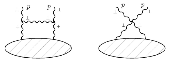
Fig. 1: The general form of the QCD diagrams for which there exists a difference between the light-front and the Lorentz-invariant calculations; $p$ is an external momentum; the symbols ”$+$” and ”$\bot$” at the lines denote the corresponding Lorentz index of the propagator.

The conditions for these diagrams to be trivially dependent on external momenta are fulfilled (see [13]); therefore, for these diagrams, the required difference is

$$\halign{\hbox to\displaywidth{$\hfil\displaystyle#\hfil$}\cr 0.0pt{\hfil$\displaystyle\hfill Cg_{AB},\hfill({\rm A}1.2)\cr}}$$

where $C$ is a constant in the limit $\varepsilon\to 0$, i.e., the dependence on external momenta is absent. There is no possible logarithmic correction $\ln(\varepsilon/u)$, because, in view of the Lorentz invariance in the space of $k_{+}$ and $k_{-}$, which holds for the Lagrangian, the quantity $u$ must behave like the ”$-$”-component of a vector, but there are no such expressions. There could only be the component of an external momentum, but, we already know that there is no dependence on it. Therefore, all the difference is compensated by adding the term of the form

$$\halign{\hbox to\displaywidth{$\hfil\displaystyle#\hfil$}\cr 0.0pt{\hfil$\displaystyle\hfill A^{a}_{\mu}g^{\mu\nu}A^{a}_{\nu},\hfill({\rm A}1.3)\cr}}$$

to the Lagrangian, i.e., by redefining the coefficient $c_{2}$ in formula (1.  Introduction).

Appendix 2

We analyze the possibility of the occurrence of the essential IR divergences (i.e., those occurring at any value of the external momenta) in the Feynman diagrams in the Euclidean space. We consider two cases of the divergences: when integrating over only the longitudinal momenta (they can appear because of (the term proportional to $k_{+}/k_{\scriptscriptstyle\|}^{2}$ in the gluon propagator) and when integrating over all momenta (the factors $1/k^{2}$ in the propagators also contribute to these divergences).

First case. We study whether a divergence exists if a part (or all) of the longitudinal loop momenta tend to some finite values. We assume that the external momenta do not take the special values (where the sum of a part of them is equal to zero). In addition, we assume that the transverse loop momenta are such that for all of the propagator momenta, we have $Q_{\bot}\neq 0$ (if this condition is violated, we must take the extra contribution from $d^{2}Q_{\bot}$ into account; this is the second case). Then the divergence can arise only if for some gluon line, we have $Q_{\scriptscriptstyle\|}=0$. The factor in the integrand producing the possible divergence has the form

$$\halign{\hbox to\displaywidth{$\hfil\displaystyle#\hfil$}\cr 0.0pt{\hfil$\displaystyle\hfill\frac{Q_{\mu}n_{\nu}+Q_{\nu}n_{\mu}}{Q_{\alpha}n^{\alpha}}=-\sqrt{2}\frac{(Q_{\mu}n_{\nu}+Q_{\nu}n_{\mu})(iQ_{0}+Q_{3})}{Q_{0}^{2}+Q_{3}^{2}}\hfill({\rm A}2.1)\cr}}$$

and is a pole of an order not higher than one. In the loop momentum space, we consider a point where $Q_{\scriptscriptstyle\|}=0$ for a certain set of lines. We look for the power $\sigma$ of the IR divergence. Every line of this set contributes $-1$ (if it carries the labels $+\bot$, see (Appendix 2)) or $0$ (if it carries the labels $\bot\bot$ or $++$). We exclude all lines with the labels $\bot\bot$ and $++$; then every line of the set contributes $-1$. The differentials $d^{2}q_{\scriptscriptstyle\|}$ of the loop momenta (the integration volume elements) give a positive contribution to $\sigma$. We must consider only those loop momenta whose change (other momenta being fixed) violates the condition $Q_{\scriptscriptstyle\|}=0$ for the lines of the set. The number of such loop momenta is the number of lines whose momenta can be taken arbitrarily, i.e., the number of independent lines. The total positive contribution to $\sigma$ is equal to twice this number. We then find other contributions to the IR divergence.

We break all lines of the set. The diagram splits into $n+1$ connected parts ($n=0,1,\dots$). All momenta external with respect to the whole diagram enter one part (the external momenta would otherwise take the special values). We call this part separated and the other parts nonseparated.

A nonseparated part is a subdiagram; if it has the external Lorentz labels, then it must be proportional to its external line momenta carrying these labels. But the factor of proportionality cannot contribute to $\sigma$, because of the Lorentz invariance, the invariance with respect to multiplying $n^{\mu}$ by a complex number, and the condition $Q_{\bot}\neq 0$. Every external line carrying the label $k$ ($k=1,2$) gives the factor $k^{k}$ or $g^{\mu k}$; the line carrying the label ”$+$” gives the factor $k^{+}$, where $k$ is a linear combination of the external momenta of the subdiagram, i.e., the momenta of the set lines. Therefore, every external line carrying the label ”$+$” contributes $+1$ to $\sigma$, and one carrying the label $k$ contributes zero. Let $m$ be a summary contribution to $\sigma$ obtained in such a way from the nonseparated parts.

Let $s$ be the number of lines of the set and $r$ be the number of lines of the set external with respect to the separated part. Every line carries the label ”$+$” at one end; therefore, we have

$$\halign{\hbox to\displaywidth{$\hfil\displaystyle#\hfil$}\cr 0.0pt{\hfil$\displaystyle\hfill m\geq s-r.\hfill({\rm A}2.2)\cr}}$$

The number of the independent lines in the set is equal to $s-n$ (each of the $n+1$ parts gives the $\delta$-function, and one $\delta$-function is common to the whole diagram). By the definition of $\sigma$, we have

$$\halign{\hbox to\displaywidth{$\hfil\displaystyle#\hfil$}\cr 0.0pt{\hfil$\displaystyle\hfill\sigma=2(s-n)+m-s.\hfill({\rm A}2.3)\cr}}$$

Using (Appendix 2), we obtain

$$\halign{\hbox to\displaywidth{$\hfil\displaystyle#\hfil$}\cr 0.0pt{\hfil$\displaystyle\hfill\sigma\geq 2(s-n)-r.\hfill({\rm A}2.4)\cr}}$$

Every nonseparated part has a minimum of two external lines. This means that all parts (separated and nonseparated) together have a minimum of $2n+r$ external lines of the set. All these lines are pairwise connected with each other. Consequently, we have

$$\halign{\hbox to\displaywidth{$\hfil\displaystyle#\hfil$}\cr 0.0pt{\hfil$\displaystyle\hfill s\geq\frac{1}{2}(2n+r)=n+\frac{r}{2},\hfill({\rm A}2.5)\cr}}$$

whence we obtain $\sigma\geq 0$, i.e., the divergence cannot be worse than logarithmic.

We find the general case producing this divergence. In this case, all the above-cited inequalities must reduce to equalities, i.e., we have $m=s-r$, and all the nonseparated parts are two-point diagrams. The general form of such a diagram is shown in Fig. 2.

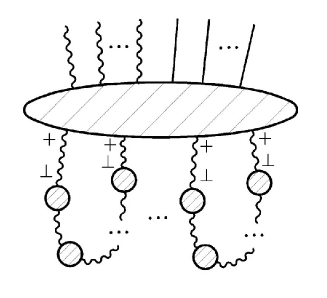
Fig. 2: The general form of the diagram producing the essential IR divergence in QCD; the symbols ”$+$” and ”$\bot$” by the lines mean that the propagator has the corresponding Lorentz index.

In this diagram every chain giving essential IR divergences contains the factor

$$\halign{\hbox to\displaywidth{$\hfil\displaystyle#\hfil$}\cr 0.0pt{\hfil$\displaystyle\hfill\Delta_{+\rho}G^{\rho\nu}\Delta_{\nu\alpha},\hfill({\rm A}2.6)\cr}}$$

where $G^{\rho\nu}$ is the nearest to the separated part nonseparated one which is one-particle irreducible subdiagram and $\Delta$ are the propagators of the lines entering to the $G^{\rho\nu}$. The divergence takes place only when the index $\rho$ in (Appendix 2) takes values $1,2$.

Second case. We now assume that a part or all of the four-dimensional momenta lend to certain finite values. The consideration is similar. The gluon propagator now gives a pole of the second order, whereas the fermion propagator gives no poles, because of the presence of the mass. Notice, that at the investigation of IR divergences one can replace all fermion lines by $1/M$ which makes impossible getting $1/M$ to the numerator. Besides in this case one can replace $R$ by 1 and $\hat{\mu}^{2}$ by $\mu^{2}$ in the propagator of gluon which excludes $\Lambda$ from the consideration. That is why from dimensional considerations, it follows that every nonseparated part contributes no less than four minus the number of its external lines to $\sigma$. This is also true for the divergent diagrams with the stipulation that for the two-point diagram, we must subtract the part independent of the momentum and proportional to $g^{\mu\nu}$ together with the divergent part, i.e., we must normalize the gluon mass to zero in every order. The latter does not violate the Ward identities in the limit of removing the regularization. Therefore, we now have

$$\halign{\hbox to\displaywidth{$\hfil\displaystyle#\hfil$}\cr 0.0pt{\hfil$\displaystyle\hfill m\geq 4n-(2s-r),\hfill\phantom{({\rm A}2.7)}\cr 0.0pt{\hfil$\displaystyle\hfill\sigma=4(s-n)+m-2s,\hfill({\rm A}2.7)\cr}}}$$

whence we obtain

$$\halign{\hbox to\displaywidth{$\hfil\displaystyle#\hfil$}\cr 0.0pt{\hfil$\displaystyle\hfill\sigma\geq r>0,\hfill({\rm A}2.8)\cr}}$$

i.e., there is no divergence.

Appendix 3

In the framework of the perturbation theory constructed based on Lagrangian (1.  Introduction)-(1.  Introduction), we consider an arbitrary diagram with three gluon external lines and investigate its structure with respect to the labels of the global gauge group. This structure has the form $A^{abc}$. The gluon propagator is proportional to $\delta^{ab}$, the three-point gluon vertex is proportional to $f^{abc}$, and the four-point vertex is proportional to $f^{abe}f^{cde}$ or $\delta^{ab}\delta^{cd}$. In addition, there can be fermion loops.

Every fermion loop gives the factor

$$\halign{\hbox to\displaywidth{$\hfil\displaystyle#\hfil$}\cr 0.0pt{\hfil$\displaystyle\hfill{\rm ReTr}(\lambda^{a}\dots\lambda^{c}),\hfill({\rm A}3.1)\cr}}$$

if the number of vertices in the loop is even or

$$\halign{\hbox to\displaywidth{$\hfil\displaystyle#\hfil$}\cr 0.0pt{\hfil$\displaystyle\hfill i{\rm ImTr}(\lambda^{a}\dots\lambda^{c}),\hfill({\rm A}3.2)\cr}}$$

if this number is odd (similar to the Furry theorem in quantum electrodynamics). We consider only the factors related to the gauge labels. From (1.  Introduction), it follows that

$$\halign{\hbox to\displaywidth{$\hfil\displaystyle#\hfil$}\cr 0.0pt{\hfil$\displaystyle\hfill\lambda^{a}_{\alpha\beta}\lambda^{a}_{\gamma\delta}=2\left(\delta_{\alpha\delta}\delta_{\beta\gamma}-\frac{1}{3}\delta_{\alpha\beta}\delta_{\gamma\delta}\right).\hfill({\rm A}3.3)\cr}}$$

We can also write

$$\halign{\hbox to\displaywidth{$\hfil\displaystyle#\hfil$}\cr 0.0pt{\hfil$\displaystyle\hfill{\rm Tr}\left(\lambda^{a}\lambda^{b}\lambda^{c}\right)=i2f^{abc}+2d^{abc},\hfill({\rm A}3.4)\cr}}$$

whence it follows that

$$\halign{\hbox to\displaywidth{$\hfil\displaystyle#\hfil$}\cr 0.0pt{\hfil$\displaystyle\hfill f^{abc}=-\frac{i}{4}\left({\rm Tr}\left(\lambda^{a}\lambda^{b}\lambda^{c}\right)-{\rm Tr}\left(\lambda^{c}\lambda^{b}\lambda^{a}\right)\right).\hfill({\rm A}3.5)\cr}}$$

We replace all $f^{abc}$ in the diagram with the right-hand side of formula (Appendix 3) and then replace all resulting expressions of the form $\lambda^{a}\lambda^{a}$ according to formula (Appendix 3). As a result, only three matrices $\lambda$ carrying three external labels of the diagram remain. These matrices are connected with each other by their labels of the fundamental representation (because after formula (Appendix 3) is used, only the Kronecker symbols remain), i.e., $A^{abc}$ consists of terms of the form

$$\halign{\hbox to\displaywidth{$\hfil\displaystyle#\hfil$}\cr 0.0pt{\hfil$\displaystyle\hfill{\rm Tr}(\lambda^{a}\lambda^{b}\lambda^{c}).\hfill({\rm A}3.6)\cr}}$$

After using formula (Appendix 3), we have the factor $i^{N}$, where $N$ is the number of three-point gluon vertices. The use of formula (Appendix 3) gives no new imaginary factors. The initial expression consists of the real quantities $\delta^{ab}$ and $f^{abc}$ and the quantities (Appendix 3) and (Appendix 3), of which the first is real and the second is imaginary; therefore, it is proportional to $i^{N^{\prime}}$, where $N^{\prime}$ is the number of fermion loops with an odd number of vertices. It is easy to show that for the diagram with three gluon external lines, the quantities $N$ and $N^{\prime}$ have different parities. Therefore, for the powers of $i$ to be consistent, it is necessary that the sum of the expressions of form (Appendix 3) be imaginary, whence, using (Appendix 3), we conclude that

$$\halign{\hbox to\displaywidth{$\hfil\displaystyle#\hfil$}\cr 0.0pt{\hfil$\displaystyle\hfill A^{abc}\sim f^{abs}.\hfill({\rm A}3.7)\cr}}$$

We now similarly consider the structure of an arbitrary diagram with four gluon external lines. It has the form $A^{abcd}$. The quantity $A^{abcd}$ consists of terms of the forms ${\rm Tr}(\lambda^{a}\lambda^{b}\lambda^{c}\lambda^{d})$ and ${\rm Tr}(\lambda^{a}\lambda^{b}){\rm Tr}(\lambda^{c}\lambda^{d})$ (the latter expression is explicitly real). It is easy to show that for the diagram with four gluon external lines, the quantities $N$ and $N^{\prime}$ have the same parities. Therefore, the sum of the indicated expressions, which compose $A^{abcd}$, must be real. We can represent the quantity ${\rm Tr}(\lambda^{a}\lambda^{b}\lambda^{c}\lambda^{d})$) as a sum of its symmetrized part (explicitly real) and expressions of the form $if^{abe}{\rm Tr}(\lambda^{c}\lambda^{d}\lambda^{e})$. In view of the reality condition, the latter expression must be a sum of quantities of the form $f^{abe}f^{cde}$. Direct calculation shows that the symmetrized part of the quantity ${\rm Tr}(\lambda^{a}\lambda^{b}\lambda^{c}\lambda^{d})$ is proportional to the symmetrized part of the quantity $\delta^{ab}\delta^{cd}$. We can therefore conclude that $A^{abcd}$ consists of terms of the forms

$$\halign{\hbox to\displaywidth{$\hfil\displaystyle#\hfil$}\cr 0.0pt{\hfil$\displaystyle\hfill f^{abc}f^{abc}\quad{\rm and}\quad\delta^{ab}\delta^{cd}.\hfill({\rm A}3.8)\cr}}$$

Appendix 4

We shall find a form of the values which are necessary to add to Feynman diagrams in order to in the limit $\Lambda\to\infty$ make them finite and coincident with its value calculated using dimensional regularization. We consider a diagram in Euclidean space constructed from propagator (3.  Comparison of the light-front and Lorentz-invariant perturbation theories), from the propagator $\Delta^{\psi}$, and from the vertices entering (3.  Comparison of the light-front and Lorentz-invariant perturbation theories) with restrictions (1.  Introduction) removed. The other vertices entering (1.  Introduction) are involved only in reducing the subdiagrams of the preceding orders of the perturbation theory to the ”correct” (i.e., calculated using dimensional regularization) value including cancellation of divergences.

It is clear that the summary fermion propagator can be represented as

$$\halign{\hbox to\displaywidth{$\hfil\displaystyle#\hfil$}\cr 0.0pt{\hfil$\displaystyle\hfill\Delta^{\psi}=\frac{k_{\mu}\gamma^{\mu}}{k^{2}-M_{0}^{2}+i0}R^{\prime}+\frac{M_{0}}{k^{2}-M_{0}^{2}+i0}R^{\prime\prime},\hfill({\rm A}4.1)\cr}}$$

where $R^{\prime}$ and $R^{\prime\prime}$ are cutoff factors that properly decrease and $R^{\prime},R^{\prime\prime}\mathrel{\mathop{\longrightarrow}\limits_{\Lambda\to\infty}}1$. We represent the diagram as a sum such that one summand contains only one term of the numerator of every fermion propagator. Each of these summands can be represented as

$$\halign{\hbox to\displaywidth{$\hfil\displaystyle#\hfil$}\cr 0.0pt{\hfil$\displaystyle\hfill I=\int dkF(k,p)f_{\Lambda}(k,p),\hfill({\rm A}4.2)\cr}}$$

where $dk$ represents all volume elements, $f_{\Lambda}(k,p)$ is the product of all factors $R^{\prime}$ and $R^{\prime\prime}$ entering tlie fermion propagators and of all factors $R$ entering boson propagators (3.  Comparison of the light-front and Lorentz-invariant perturbation theories), $k$ denotes the integration momenta, and $p$ denotes the external momenta of the diagram.

It is evident that we can find a function $\hat{F}(k,p)$ that is polynomial in $p$, is Lorentz invariant, and has no nonintegrable IR singularities such that for $\hat{F}(k,p)$ and $F(k,p)$, a number of the first terms of their asymptotic expansions at infinity with respect to $k$ coincide and the difference $F(k,p)-\hat{F}(k,p)$ is integrable (see the refinement below). Therefore, we can write

$$\halign{\hbox to\displaywidth{$\hfil\displaystyle#\hfil$}\cr 0.0pt{\hfil$\displaystyle\hfill I=\int dk(F(k,p)-\hat{F}(k,p))f_{\Lambda}(k,p)+\int dk\hat{F}(k,p)f_{\Lambda}(k,p).\hfill({\rm A}4.3)\cr}}$$

Up to corrections of the order $1/\Lambda$, we can neglect the factor $f_{\Lambda}(k,p)$ in the first integral (because the integral converges even in the absence of this factor). We can then assume that this integral is calculated using dimensional regularization and we can split it into two integrals (assuming that they are both renormalized by dimensional regularization). As a result, we obtain the expression

$$\halign{\hbox to\displaywidth{$\hfil\displaystyle#\hfil$}\cr 0.0pt{\hfil$\displaystyle\hfill I=\int^{dim}dkF(k,p)-\int^{dim}dk\hat{F}(k,p)+\int dk\hat{F}(k,p)f_{\Lambda}(k,p).\hfill({\rm A}4.4)\cr}}$$

Using the expansion for the function $f_{\Lambda}(k,p)$ in the last integral in (Appendix 4) with respect to $p$ in the neighborhood of the origin (this expansion is well defined for any $k$), we can now show that the last integral in (Appendix 4) is a polynomial in $p$ plus corrections of the order $1/\Lambda$.

We must make the following refinement of these considerations. Before subtracting the overall divergence of the diagram, we must verify that the diagram has no subdivergences with respect to a part of the integration variables. Such subdivergences can be produced by subdiagrams (which is taken into account by the renormalization in the lower orders) or by the divergence on integrating over a part of the momentum components. For the QCD in the gauge $A_{-}=0$, the latter is possible because of the improper decrease of the propagator in the direction $k_{\bot}$. It is known [24] that this divergence is present if the index of the UV divergence with respect to a part of the components is nonnegative. From the structure of the propagators, we can see that in the Euclidean space, the subtraction of the overall divergence cannot decrease only the index $\omega_{\bot}$ of the UV divergence with respect to $k_{\bot}$. This results in the necessity to preliminarily subtract, the subdivergence with respect to $k_{\bot}$, the subdivergence being in general dependent on the projections $p^{\nu}n_{\mu}$ of the external momenta in an arbitrary nonpolynomial way. Analysis of the diagrams for the Green’s functions shows that we have $\omega_{\bot}\geq 0$ for only the one-loop two-point diagrams and that $\omega_{\bot}=0$. These diagrams have only one external momentum. Therefore, they cannot have a nonpolynomial dependence on $p^{\nu}n_{\nu}$, because of the invariance with respect to multiplying the vector $n_{\nu}$ by a complex number. One must take into account that, for the diagrams of the Green’s functions, the vector $n_{\nu}$ with the nonconvolute index $\nu$ cannot stand in the numerator, because this gives zero on convolution with the propagators. If we consider the one-particle irreducible vertex parts, whose diagrams do not satisfy the last condition, the divergent parts can be nonpolynomial [18, 19], and the number of diagrams that are divergent with respect to $k_{\bot}$ can be much larger.

It seems that if the integral of the form, described at the beginning of this Appendix, converges then the result of it’ s calculation cannot depend on the vector $n^{*}_{\nu}$ (complex conjugated to $n_{\nu}$ up to a factor). But this would be true only if this integral be an analitical function of the complex vector $n_{\nu}$. However the derivative of our integral with respect to complex vector $n_{\nu}$ can be nonconvergent due to the rising of infrared singularity (of the power of the pole in $(nk)$). Therefore the result of the calculation of the diagram, and, hence, it’s divergent part can depend on $n_{\nu}$ and on $n^{*}_{\nu}$. It is seen from the equation (3.  Comparison of the light-front and Lorentz-invariant perturbation theories) for the propagator that the integrands we considered are invariant with respect to a multiplication of the vector $n_{\nu}$ by a complex number (and of the $n^{*}_{\nu}$ by complex conjugate number). This allows to conclude that up to corrections of the order $1/\Lambda$ the difference between the diagram described in the beginning of this appendix (more precisely, the finite sum of such diagrams of the given order) and its value calculated using dimensional regularization (i.e., the similar sum of the first integrals in (Appendix 4)) reduces to a polynomial in the external momenta with coefficients containing factors $N_{\alpha\beta}$ (see the definition of this value in formula (1.  Introduction)).

References

- [1] V. A. Fock, Z. Phys., 75, 622 (1932); 76, 852 (1932); Papers on Quantum Field Theory [in Russian], Izd. Leningr. Univ., Leningrad (1957).
- [2] I. E. Tamm. J. Phys. USSR, 9, 449 (1945).
- [3] S. M. Dancoff, Phys. Rev., 78, 382 (1950).
- [4] P. A. M. Dirac, Rev. Mod. Phys., 21, 392 (1949).
- [5] A. A. Logunov and A. N. Tavkhelidze, Nuovo Cimento, 29, 370 (1963).
- [6] V. G. Kadyshevskii and A. N. Tavkhelidze, ”Quasi-potential method for the relativistic two-body problem,” in: Problems of Theoretical Physics (Dedicated to N. N. Bogoliubov in honor of his 60th birthday) (D. I. Blokhintsev et al., eds.) [in Russian], Nauka, Moscow (1969), p. 261.
- [7] R. N. Faustov. Theor. Math. Phys., 3, 478 (1970); Ann. Phys., 78, 176 (1973).
- [8] V. R. Garsevamshvili et al., Theor. Math. Phys., 23, 533 (1975).
- [9] V. A. Karmanov, Fiz. Elem. Chast. At. Yadra, 19, 525 (1988).
- [10] E. Tomboulis, Phys. Rev. D, 8, 2736 (1973).
- [11] A. Cacher. Phys. Rev. D, 14, 452 (1976).
- [12] V. A. Franke, Yu. V. Novozhilov, E. V. Prokhvatilov, Lett. Math. Phys., 5, 437 (1981).
- [13] S. A. Paston and V. A. Franke, Theor. Math. Phys., 112, 1117 (1997), hep-th/9901110.
- [14] M. Burkardt and A. Langnau, Phys. Rev. D, 44, 1187, 3857 (1991).
- [15] M. Burkardt, Adv. Nucl. Phys., 23, 1 (1996).
- [16] K. G. Wilson, T. S. Walhout, A. Harindranath, W.-M. Zhang, R. J. Perry and S. D. Glazek, Phys. Rev. D, 49, 6720 (1994).
- [17] B. H. Allen and R. J. Perry, Phys. Rev. D, 58, 125017 (1998).
- [18] A. Basseto, M. Dalbosko and R. Soldati, Phys. Rev. D, 36, 3138 (1987).
- [19] A. Basseto, G. Nardelli and R. Soldati, Yang-Mills Theories in Algebraic Noncovariant Gauges, World Scientific, Singapore (1991).
- [20] S. Mandelstam, Nucl. Phys. B, 213, 149 (1983).
- [21] G. Leibbrandt, Phys. Rev. D, 29, 1699 (1984).
- [22] W.-M. Zhang and A. Harindranath, Phys. Rev. D, 48, 4868, 4881, 4903 (1993).
- [23] N. E. Ligterink and B. L. G. Bakker Phys. Rev. D, 52, 5954 (1995).
- [24] S. Weinberg, Phys. Rev., 118, 838 (1960).
- [25] C. Acerbi and A. Basseto, Phys. Rev. D, 49, 1067 (1994).