NON-ABELIAN FIELD THEORY OF STABLE NON-BPS BRANES

Abstract:

We derive the action for the non-abelian field theory living on parallel non-BPS D3-branes in type IIA theory on the orbifold ${\bf T}^{4}/{{\cal{I}}_{4}(-1)^{F_{L}}}$. The classical moduli space for the massless scalars originating in the “would be” tachyonic sector shows an interesting structure. In particular, it contains non-abelian flat directions. At a generic point in this branch of the moduli space the scalars corresponding to the the separations of the branes acquire masses and the branes condense. Although these tree level flat directions are removed by quantum corrections we argue that within the loop approximation the branes still condense.

1 Introduction

Non-BPS branes in type II string theory [1, 2] have recently attracted considerable attention. On one hand they are of interest because the are stable, non-perturbative states in string theory without preserving any supersymmetry. These states are therefore important to gain a deeper understanding of the non-perturbative spectrum of string theory. On the other hand, BPS D-branes have played a key role in the recent success of describing non-perturbative properties of supersymmetric Yang-Mills theory in terms of string theory [3]. The hope is now that non-BPS states could play a similarly important role in the analysis of non-perturbative properties of non-supersymmetric Yang-Mills theory. Previous work in this direction has focused on D-branes in non-supersymmetric type 0 theory [4]. A successful generalisation of the AdS/CFT correspondence [5] to these non-supersymmetric backgrounds of a stack of D-branes has however been hampered by the tachyonic instability in the closed string sector of that theory [6].

In Sen’s non-BPS branes of type II theory such instabilities in the closed string sector are absent. Instead one has to deal with a tachyon in the open string sector. However, it turns out that these instabilities can be cured by considering type II theory on an appropriate orbifold. In doing so stable non-BPS branes have been obtained [1, 2]. While the possible application of these objects for a string-theoretic description of non-supersymmetric, non-abelian field theory has been suggested [1] we are not aware of any concrete progress in this direction.

In this paper we initiate a systematic analysis of the low energy dynamics of a stack of non-BPS branes in type II theory. In particular we construct the low energy effective field theory on a stack of non-BPS 3-branes. Before proceeding it is perhaps necessary to clarify some subtleties that arise in the present situation. It has been argued that generically there is a force between two non-BPS branes generated at loop one loop in open string theory [8]. If so, a stack of non-BPS branes is unstable. In such a situation it is not clear that the effective field theory is appropriate. Indeed one motivation for our work is to address this question in a concrete example. In this paper we shall determine the low energy interactions of the light fields from tree-level string theory. The effective action is then simply defined to be a local quantum field theory of these light modes which reproduces the correct amplitudes. It turns out that, as in the supersymmetric case, many of the couplings such as the gauge couplings can be inferred solely from geometrical considerations and T-duality. In addition, the Yukawa couplings are restricted by general properties of the string S-matrix such as winding number conservation. In this way one can fix all couplings apart from the potential for the scalars $\chi_{i}$ originating in the tachyonic sector. These in turn will be fixed below by an explicit calculation of the four-tachyon amplitude in the presence of non-BPS branes. The potential obtained in this way shows some interesting features. The four scalar interaction ($[\chi_{i},\chi_{j}]^{2}$) always present in supersymmetric theories arises also in the potential for $\chi_{i}$, but with the opposite sign! The corresponding instability is however cured by another $\chi^{4}$-term that comes with exactly the right coefficient to transform this instability into a flat direction of the potential. Note however, that contrary to supersymmetric theories, these new flat directions do not lie in the commuting Cartan subalgebra. As a consequence, unlike in the supersymmetric case, at a generic point in this branch of the moduli space all scalars corresponding to the separations of the branes acquire masses. This in turn leads to a condensation of the non-BPS branes. Nevertheless, the gauge symmetry is spontaneously broken.

We then discuss how quantum corrections affect these flat directions within the field theory approximation. In vacua where $\chi_{i}\!=\!0$ the one-loop correction to the potential for the scalars $\phi_{I}$ (corresponding to separating the non-BPS branes) leads to a repulsive force, unless the orbifold is tuned in such a way that the masses of the scalars from the tachyonic sector vanish. This is in agreement with a one-loop open string calculation [8] and is a result of a Bose-Fermi degeneracy. However we will see that this degeneracy does not persist at the level of the interacting field theory and therefore we suspect that the effective potential will not vanish at two loops at the critical radii. We also consider the one loop correction to the effective potential for the scalars $\chi_{i}$, which removes all flat directions in the corresponding branch when $m_{i}=0$. The new minimum prefers a non-vanishing, non-abelian expectation value of $\chi_{i}$. This, in turn induces a mass term for other scalars $\phi_{I}$ resulting in an attractive force between the branes. This raises the possibility that a stack of non-BPS branes can condense even when the orbifold is not tuned precisely to criticality. This is encouraging in view of a possible existence of a gravitational background dual to the field theory on the branes. Indeed, a necessary condition for a successful description of non-Abelian YM-theory in terms of these non-BPS branes is, of course, that a stack of such branes is stable, i.e. does not fly apart. Our result for the field theory action of these branes provides sufficient information to further verify this condition at higher order. We leave this lengthy but, in principle straightforward computation for future work.

The rest of this paper is organised as follows. In section two we review some basic features of non-BPS 3-branes in type IIA string theory. In section three we determine the low energy field theory on parallel branes. Lastly in section four we calculate the one-loop corrections to the effective potentials for the scalar fields.

2 Non-BPS 3-branes

In this section we review the basic features of stable non-BPS branes in type II string theory. We will consider a non-BPS 3-brane in type IIA string theory for the sake of clarity. However, the generalisation to other branes is clear. We use a “mostly plus” metric and the conventions that indices $m,n=0,1,2,...,9$ run over all of ten-dimensional space-time, $\mu,\nu=0,1,2,3$ run over the 3-brane world volume, $i,j=6,7,8,9$ and $I,J=4,5$ label the transverse directions. Group indices are labeled by $a,b$ and we choose a hermitian basis with $\hbox{Tr}(t^{a}t^{b})=\delta^{ab}$. We will suppress all spinor indices.

As explained in [1] the excitations of a single non-BPS D-brane are carried by two types of open strings with CP factor $I$ and $\sigma_{1}$ respectively. The CP $I$-sector is precisely the same as for a BPS D-brane and gives rise to massless $N=4$ vector multiplet $A_{\mu},\phi^{I},\chi^{i},\lambda$ on the brane. Here $\lambda$ is a ten-dimensional spinor which, as a consequence of the GSO projection, is chiral (in a ten-dimensional sense). If there are $N$ branes then the gauge group is $U(N)$. The CP $\sigma_{1}$ sector has GSO-projection $(-1)^{F}\!=\!-1$ and hence contains a tachyonic state in its spectrum. The lightest modes are therefore a (real) tachyon $\tau$ with $m^{2}=-\frac{1}{2\alpha^{\prime}}$ from the NS ground state and a massless a ten-dimensional fermion $\psi$ from the R ground state. The two fermions $\lambda$ and $\psi$ have opposite ten-dimensional chirality. All fields are in the adjoint of $U(N)$.

The tachyonic instability of the non-BPS brane can be removed by compactifying the directions $x^{i}\cong x^{i}+R_{i}$ and introducing an orbifold $T^{4}/{\cal I}_{4}(-1)^{F_{L}}$, where ${\cal I}_{4}:x^{i}\mapsto-x^{i}$ and $F_{L}$ is the left-moving spacetime fermion number. The effect of this orbifold in the $I$-sector is simply to remove the scalars $\phi^{i}$ and project onto six-dimensional chiral fermions $\lambda_{+}$, $\Gamma^{6789}\lambda_{+}=\lambda_{+}$. This leaves an $N=2$ vector multiplet in four dimensions. In the $\sigma_{1}$-sector the ${\cal I}_{4}$ also projects on to six-dimensional chiral fermions $\psi_{-}$, $\Gamma^{6789}\psi_{-}=\psi_{-}$. In addition ${\cal I}_{4}$ reverses the sign of the tachyon winding modes and the orbifold keeps only those components which are odd under ${\cal I}_{4}$. Thus after the orbifold the lightest field in the NS sector with CP-factor $\sigma_{1}$ originates in the ground state of strings with winding number one around the coordinate $x_{i}$. As there are four compact directions we will have eight different scalar fields $\tau_{i}^{\pm}$ associated with these modes, where $\tau_{i}^{\pm}$ is the component of the tachyon with winding number $\pm 1$ around $x^{i}$. In particular only the combinations

$$\chi_{i}={\tau_{i}^{+}-\tau_{i}^{-}\over\sqrt{2}}\ ,$$ (1)

survive. Their mass is given by

$$m_{i}^{2}=\left({R_{i}\over\alpha^{\prime}}\right)^{2}-{1\over 2\alpha^{\prime}}\ ,$$ (2)

where $R_{i}$ is the radius of the compact direction $x^{i}$. Thus, so as long as $R_{i}\geq R_{c}\!=\!\sqrt{\frac{\alpha^{\prime}}{2}}$, these lowest mass states are not tachyons and hence a non-BPS brane is stable. On the other hand we can tune the radii so that the $m_{i}^{2}$ are small compared to the string scale. Therefore these states are relevant for the low energy dynamics and should be included in the field action of the brane.

To summarise, after the orbifold, the light fields on the non-BPS branes consist of an $N=2$ vector multiplet $(A_{\mu},\phi^{I},\lambda_{+})$ with gauge group $U(N)$ coupled to a massless six-dimensional fermion $\psi_{-}$ and four massive scalars $\chi_{i}$ all in the adjoint representation. Note that at the critical radius we obtain the field content of an $N=4$ super-Yang-Mills gauge theory. However we will shortly see that the interactions of these fields are never supersymmetric.

3 Non-Abelian action for non-BPS 3-branes

In [10] Sen proposed a world volume action for a single non-BPS p-brane of the form

$$S=T_{p}\int d^{4}\sigma\sqrt{|G_{ab}+B_{ab}+2\pi\alpha F_{ab}|}[\sum_{i}(\partial\chi)^{2}-V(\chi)]+\ldots,$$ (3)

where $V(\chi)\!=\!1+m^{2}\chi^{2}+O(\chi^{3})$ and the ellipses denote fermionic terms. We now want to find the non-Abelian action describing a stack of non-BPS 3-branes of type IIA string theory on the orbifold $T^{4}/{\cal I}_{4}(-1)^{F_{L}}$. For this we first recall that the fields originating in the CP-factor $I$ are the same as for a BPS-brane. Therefore the action for these fields is the same as for the BPS case, i.e. an $N=2$, $U(N)$ gauge theory. For the fields originating in the $\sigma_{1}$-sector some parts of the action (namely those up to $O(\chi^{2})$) can, in fact, be obtained from geometric considerations and T-duality alone as we shall now demonstrate.

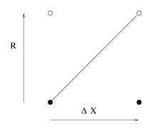
Figure 1: Open string stretching between two D0-branes while winding once around the orbifold with radius $R$

Consider for example a pair of non-BPS D0-branes, separated by a distance $\Delta X_{1}$, and a $\sigma_{1}$-string starting at one $D0$ wrapping around the orbifold and ending on the other $D0$. The mass of such a string is given by

$$M^{2}_{i}=\left(\frac{\Delta X}{\alpha^{\prime}}\right)^{2}+{N-{1\over 2}\over\alpha^{\prime}}\ ,$$ (4)

where $N$ is the oscillator number of the string state. Now, from (Fig. 1) $(\Delta X)^{2}\!=\!(R_{i})^{2}+(\Delta X_{i})^{2}$. This mass must then be reproduced within the world volume theory. A similar argument applies to the mass of $\psi_{-}$ which is non-zero if the $\sigma_{1}$ string is stretched (with no $-{1\over 2}$ in (4)). Thus, after rescaling the fields to the canonical dimensions in field theory we conclude that the effective action has the form

$$S = {\rm Tr}\int\;\hbox{d}^{4}x\left[\frac{1}{4}F_{\mu\nu}F^{\mu\nu}+{1\over 2}(D_{\mu}\phi_{I})(D^{\mu}\phi^{I})-\frac{g_{\hbox{\tiny YM}}^{2}}{4}([\phi^{I},\phi^{J}])^{2}\right.$$

$$\qquad\qquad\qquad\left.-{ig_{\hbox{\tiny YM}}}\bar{\lambda}_{+}\Gamma^{\mu}D_{\mu}\lambda_{+}+g_{\hbox{\tiny YM}}\bar{\lambda}_{+}\Gamma^{I}[\phi^{I},\lambda_{+}]\right.$$

$$\qquad\qquad\qquad\left.+{1\over 2}(D_{\mu}\chi_{i})(D^{\mu}\chi^{i})+{1\over 2}m_{i}^{2}\chi_{i}^{2}-\frac{g_{\hbox{\tiny YM}}^{2}}{2}[\phi^{I},\chi_{i}][\phi^{I},\chi^{i}]\right.$$

$$\qquad\qquad\qquad\left.-{ig_{\hbox{\tiny YM}}}\bar{\psi}_{-}\Gamma^{\mu}D_{\mu}\psi_{-}+g_{\hbox{\tiny YM}}\bar{\psi}_{-}\Gamma^{I}[\phi^{I},\psi_{-}]+{\cal L}_{\sigma_{1}}\right]\ ,$$

where ${\cal L}_{\sigma_{1}}$ denotes additional terms involving fields from the $\sigma_{1}$-sector and $D_{\mu}=\partial_{\mu}+ig_{\hbox{\tiny YM}}[A_{\mu},\ ]$ is the gauge covariant derivative. For simplicity we continue to label the fermions in terms of ten dimensional spinors and therefore the $\Gamma$-matrices are also ten-dimensional. In this notation $\lambda_{+}$ and $\psi_{-}$ are constrained to have opposite ten-dimensional chiralities and the subscript $\pm$ refers to their chirality under $\Gamma^{012345}$. This action reproduces the correct masses for the scalars $\phi_{I}$ in the CP factor $I$ and the tachyons $\chi_{i}$ in the CP factor $\sigma_{1}$. The covariant derivative arises because the $\sigma_{1}$-sector fields are in the adjoint. This also follows via T-duality of the couplings $[\phi_{I},\chi_{i}][\phi^{I},\chi^{i}]$ and $\bar{\psi}_{-}\Gamma^{I}[\phi^{I},\psi_{-}]$ in (3). Alternatively, one can deduce the $([\phi_{I},\chi_{i}])^{2}$ and $\bar{\psi}_{-}[\phi_{I},\psi_{-}]$ couplings from T-duality and fact that $\chi$ and $\psi$ are in the adjoint.

Next we determine the remaining terms ${\cal L}_{\sigma_{1}}$ that appear in (3). Let us first discuss the fermion-tachyon coupling. In addition to the terms

$$\bar{\psi}_{-}\Gamma^{I}[\phi_{I},\psi_{-}]$$ (6)

in (3) one might expect, in view of the similarity of (3) with $N=4$ Yang-Mills, further Yukawa couplings involving the tachyons $\chi_{i}$. If both fermions originate in the same sector then this coupling is excluded as it involves a trace over an odd number of $\sigma_{1}$’s. On the other hand this does not exclude coupling of the form

$$\bar{\lambda}_{+}\Gamma^{k}[\chi_{k},\psi_{-}]\ .$$ (7)

Indeed precisely such a coupling occurs in an $N=4$ super-Yang-Mills action. However, this coupling is excluded in the field theory limit because, due to winding number conservation, one of the fermions would have to have a non-zero winding number and therefore a mass of $O(\alpha^{\prime})$. The absence of these terms is a first indication that (3) is never supersymmetric in contrast to the effective action for BPS D3-branes.

The only remaining undetermined term in the effective action is the potential for the scalars originating in the tachyonic NS sector

$$V(\chi_{i})=-\frac{1}{2}m_{i}^{2}\chi_{i}^{2}-{\cal L}_{\sigma_{1}}\ .$$ (8)

Since have already determined the mass term in $V(\chi_{i})$ let us concentrate on the terms $O(\chi^{3})$ and $O(\chi^{4})$. To determine the exact form of these terms one can analyse disk three-and four point functions respectively. In fact the three-point function must vanish, as can be seen in a number ways. One way is to note that the trace over an odd number of $\sigma_{1}$ vanishes. In addition winding number conservation implies that processes involving an odd number of $\chi_{i}$ fields must vanish. This leads to a ${\bf Z}_{2}^{4}$ symmetry of the effective theory generated by $\chi_{i}\leftrightarrow-\chi_{i}$. Thus we are left with the four-point function $S_{D}(k_{1},\cdots,k_{4})$. The relevant graphs for this are given in Fig. 2. The rest of this section is devoted to calculating the corresponding amplitude and deducing the form of the four-tachyon term in the effective action.

If we denote by $k$ the “field theory” momentum (i.e. momentum tangent to the brane) then the full ten-dimensional momentum $K$ of the i-th tachyon winding mode is

$$K\!=\!k+\frac{1}{\alpha^{\prime}}{\vec{w}_{i}}\ .$$ (9)

Here $\vec{w}_{i}$ is the winding vector of the tachyon around the compact directions $x^{i}$. The lowest mass states $\tau_{i}^{\pm}$ left after the orbifold have $\vec{w_{6}}=(\pm R_{6},0,0,0)$, $\vec{w_{7}}=(0,\pm R_{7},0,0)$, $\vec{w_{8}}=(0,0,\pm R_{8},0)$ and $\vec{w_{9}}=(0,0,0,\pm R_{9})$. To fix the gauge we need to fix three of the bosonic coordinates and two of the fermionic coordinates in this correlator. The fixed (-1 picture) and the integrated (0-picture) vertex operators are

$$V_{\tau}^{(0)}=i2\alpha^{\prime}gc(x)\left(K\cdot\psi(x)\right)e^{iK\cdot X(x)}\quad\hbox{{and}}\quad V_{\tau}^{(-1)}=i\sqrt{2\alpha^{\prime}}gc(x)e^{-\phi(x)}e^{iK\cdot X(x)}\ ,$$ (10)

respectively. The corresponding amplitude is found to be

$$S_{D}(k_{1},\cdots,k_{4}) = 4\alpha^{\prime}g^{2}(2\pi)^{4}\delta_{\sum\vec{w}_{i}}\delta^{4}(\sum\limits_{i=1}^{4}k_{i})\hbox{Tr}_{f}[t^{a_{1}},\cdots,t^{a_{4}}]$$

$$\cdot\frac{x_{12}x_{23}x_{13}}{x_{12}x_{34}}K_{3}K_{4}\int\limits_{-\infty}^{\infty}\hbox{d}x_{4}\;\prod\limits_{i<j}|x_{ij}|^{2\alpha^{\prime}K_{i}\cdot K_{j}}+(K_{2}\leftrightarrow K_{3}),$$

where $\delta_{\sum\vec{w}_{i}}$ ensures the winding number conservation. In terms of the ten-dimensional Mandelstam variables

$$S=-(K_{1}+K_{2})^{2}\quad\hbox{{,}}\quad T=-(K_{1}+K_{3})^{2}\quad\hbox{{,}}\quad U=-(K_{1}+K_{4})^{2},$$ (12)

with

$$S+T+U\!=\!-2/\alpha^{\prime},$$ (13)

the amplitude takes the form

$$S_{D}(k_{1},\cdots,k_{4}) = 2g^{2}(2\pi)^{4}\prod\limits_{p=1}^{4}\delta_{\sum\vec{w_{i}}}\delta^{4}(\sum\limits_{i=1}^{4}k_{i})$$

$$\cdot{\left[(1+\alpha^{\prime}U)\hbox{Tr}(t^{a_{3}}t^{a_{4}}t^{a_{2}}t^{a_{1}}+t^{a_{2}}t^{a_{4}}t^{a_{3}}t^{a_{1}})B(-\alpha^{\prime}S,-\alpha^{\prime}T)\right.}$$

$${\left.+(1+\alpha^{\prime}T)\hbox{Tr}(t^{a_{2}}t^{a_{3}}t^{a_{4}}t^{a_{1}}+t^{a_{3}}t^{a_{2}}t^{a_{1}}t^{a_{4}})B(-\alpha^{\prime}S,-\alpha^{\prime}U)\right.}$$

$${\left.+(1+\alpha^{\prime}S)\hbox{Tr}(t^{a_{3}}t^{a_{2}}t^{a_{4}}t^{a_{1}}+t^{a_{2}}t^{a_{3}}t^{a_{1}}t^{a_{4}})B(-\alpha^{\prime}T,-\alpha^{\prime}U)\right]},$$

where $B(a,b)$ is the Euler beta function. The amplitude (3) has no pole at $\alpha^{\prime}S\!=\!-{1\over 2}$. In the bosonic string this pole is related to the tachyonic intermediary state. Its absence is the consistent with the absence of a three tachyon coupling, as explained above. After orbifolding the full four-tachyon amplitude is the given by the sum over all diagrams in figure 2. Winding number conservation implies that the external states must be of the form $\tau_{i}^{+},\tau_{i}^{-},\tau_{j}^{+},\tau_{j}^{-}$. There are two cases to consider: either $i\neq j$ or $i=j$.

Figure 2: Different disc diagrams corresponding to the $4$ tachyon amplitude on the orbifold ${\bf T}^{4}/{{\cal{I}}_{4}(-1)^{F_{L}}}$

Let us first consider diagrams of Fig. 2 with $i\neq j$. Here we find that there are four separate graphs which contribute to $\chi_{i},\chi_{i},\chi_{j},\chi_{j}$ scattering. It is helpful here to introduce the Mandelstam variables for the field theory momenta

$$s=-(k_{1}+k_{2})^{2}\ ,\qquad t=-(k_{1}+k_{3})^{2}\ ,\qquad u=-(k_{1}+k_{4})^{2}\ .$$ (15)

For the four graphs of interest we find that

$$S=-1/\alpha^{\prime}+s-(m_{i}^{2}+m_{j}^{2})\ ,\qquad T=-1/\alpha^{\prime}+t-(m_{i}^{2}+m_{j}^{2})\ ,\qquad U=u\ .$$ (16)

We may now expand the amplitude (3) to lowest order in $\alpha^{\prime}$, noting that $s,t$ and $u$ are all $O(1)$. In this way we find

$$S^{ij}_{D}(k_{1},\cdots,k_{4}) = g^{2}(2\pi)^{4}\delta^{4}(\sum\limits_{i=1}^{4}k_{i})\left(\hbox{Tr}(-{1\over 2}[t^{a_{2}},t^{a_{3}}][t^{a_{1}},t^{a_{4}}]+\{t^{a_{2}},t^{a_{4}}\}\{t^{a_{1}},t^{a_{3}}\}\right.$$ (17)

$$\left.+\left({t-s\over 2u}\right)\hbox{Tr}([t^{a_{2}},t^{a_{3}}][t^{a_{1}},t^{a_{4}}])\right)\ .$$

The pole corresponds to an exchange of a gauge boson in the u-channel. Note that, for $i\neq j$, the incoming states can only annihilate to a zero winding number state such as a gauge boson in the u-channel.

Let us now consider diagrams in Fig. 2 where $i=j$. Winding number conservation now implies that there are six graphs that must be summed over. These graphs come in three pairs with

$$S=s\ ,\qquad T=t\ ,\qquad U=-2/\alpha^{\prime}+u-4m_{i}^{2}\ ,$$ (18)

and similarly for the other two pairs. If we now sum of all these contributions we find

$$S^{ii}_{D}(k_{1},\cdots,k_{4}) = g^{2}(2\pi)^{4}\delta^{4}(\sum\limits_{i=1}^{4}k_{i})\left(\left({t-s\over u}\right)\hbox{Tr}([t^{a_{2}},t^{a_{3}}][t^{a_{1}},t^{a_{4}}])\right.$$ (19)

$$\left.+\left({s-u\over t}\right)\hbox{Tr}([t^{a_{1}},t^{a_{3}}][t^{a_{2}},t^{a_{4}}])\right.$$

$$\left.+\left({t-u\over s}\right)\hbox{Tr}([t^{a_{1}},t^{a_{2}}][t^{a_{3}},t^{a_{4}}])\right)\ .$$

Thus here there are only pole contributions corresponding to the exchange of a gauge boson. Note that for $i=j$ it is possible for the incoming states to annihilate into a zero winding state in any of the three channels. Comparing (17) and (19) with the tree-level field theory amplitude we find after a lengthy but straightforward computation that the string tree-level amplitude is reproduced by the following potential for the scalars $\chi$ originating in the tachyonic sector

$$V(\chi)=\hbox{Tr}\left({1\over 2}\sum\limits_{i}m_{i}^{2}\chi^{2}_{i}+\frac{g_{\hbox{\tiny YM}}^{2}}{4}\sum\limits_{i\neq j}([\chi_{i},\chi_{j}])^{2}+g_{\hbox{\tiny YM}}^{2}\sum\limits_{i\neq j}(\chi_{i})^{2}(\chi_{j})^{2}\right)\ .$$ (20)

This is the main result of this paper. Before discussing its implications a comment about the uniqueness of the effective potential (20) is in order. As is well known the effective action for tachyons is ambiguous [11] due to the possibility of replacing $m^{2}T$ by $\nabla^{2}T$. In the present situation this ambiguity can in principle arise for the $\chi^{4}$ term and should be kept in mind for the cases when $m_{i}\neq 0$.

Let us briefly describe the classical vacuum moduli space of the theory. Of course without supersymmetry we do not expect any of these vacuum moduli to persist in the quantum theory and hence we must interpret the term moduli space loosely. We note that the complete potential for all the fields can be written as

$$\hbox{Tr}\left[-\frac{1}{2}g^{2}_{YM}([\phi_{4},\phi_{5}])^{2}-\frac{1}{2}g^{2}_{YM}\sum_{I,i}([\phi_{I},\chi_{i}])^{2}+\frac{1}{2}\sum_{i}m_{i}^{2}\chi_{i}^{2}+\frac{g^{2}_{YM}}{4}\sum_{i\neq j}(\{\chi_{i},\chi_{j}\})^{2}\right]\ .$$ (21)

Clearly if $m_{i}^{2}<0$ for some $i$, say $i=1$, then the potential is not bounded from below because we may take only $\chi_{1}$ to be non-vanishing and thereby make the potential as negative as we wish. On the other hand if $m_{i}^{2}\geq 0$ for all $i$ then since we have chosen a hermitian basis for the Lie algebra it is not hard to see that all the terms appearing in (21) are positive. Thus the potential is bounded below by zero.

For generic values of the orbifold radii the potential is minimized by $\chi_{i}=0$ and $[\phi_{4},\phi_{5}]=0$. In this case the moduli space of vacua are given by the Cartan subalgebra of $U(N)$. This corresponds to a Coulomb branch with $N$ massless $U(1)$ gauge fields.

If $m_{i}^{2}=0$ then there are additional branches of the vacuum moduli space that can arise where $\phi_{I}=0$. We are then left with the requirement $\{\chi_{i},\chi_{j}\}=0$ for $i\neq j$, $m^{2}_{i}=m^{2}_{j}=0$ (and $\chi_{i}=0$ if $m_{i}^{2}>0$), i.e. this vacuum is parameterised by anti-commuting scalar vevs. Generically in these branches the gauge group is completely higgsed leaving only the massless fields from the $U(1)$ corresponding to the overall translation invariance. Note that here the scalars $\phi_{I}$ become massive so that the non BPS-branes are bound together. In addition the ${\bf Z}_{2}^{4}$ symmetry of the theory is spontaneously broken.

4 One-Loop Effective Potential

In this section we compute within the the field theory approximation the one-loop corrections to the tree level potentials obtained in the previous section. For simplicity we take all the radii to be equal and assume that there are only two non-BPS branes. It has been shown using open string theory [8] that there is a one-loop repulsive force between the two non-BPS branes which vanishes at the critical radius $R\!=\!R_{c}$. We will reproduce this force in the field theory approximation where it corresponds to the lifting of the Coulomb branch by a one-loop effective potential for the scalars $\phi_{I}$, when the $\sigma_{1}$-scalars $\chi_{i}$ are set to zero. We will also discuss the lifting of the Higgs branch discussed above when $m=0$ and $\phi_{I}=0$. As we shall see, the one-loop quantum corrections remove the $\chi_{i}=0$ vacuum, indicating that the branes can condense.

Let us first describe the lifting of the Coulomb branch resulting in a force between the branes when $R_{i}>R_{c}$ and the scalars from the $\sigma_{1}$-sector are massive. A quick way to compute the potential is to first consider the massless limit. In this case the field content becomes the same as that of $N=4$ super-Yang-Mills. In addition the interaction terms which break supersymmetry do not contribute to the $\phi_{I}$ effective potential at one loop. Therefore the effective potential is the same as for an $N=4$ super Yang-Mills theory and hence vanishes on account of the Bose-Fermi degeneracy. Then, because the mass term only appears in the fluctuation determinant of the tachyon, the effective potential at non-zero $m$ is simply given by

$$V_{eff}(X_{1})=2\left[\log\det(M_{m})-\log\det(M_{0})\right],$$ (22)

where ${\cal M}_{m}\!=\!-{1\over 2}g_{ab}\delta_{ij}(-\nabla^{2}+m_{i}^{2})$ is the fluctuation operator for the scalars in the $\sigma_{1}$-sector. We use the $\zeta$-function definition of the regularised functional determinants. The one-loop effective potential is then found to be $(\phi_{I}^{a}\to\delta^{a3}\delta_{I5}F+\phi_{I}^{a})$

$$2\pi^{2}V_{eff}(F) = -(m^{2}+4g_{\hbox{\tiny YM}}^{2}F^{2})^{2}\left[\frac{3}{2}-\ln\left(\frac{m^{2}+4g_{\hbox{\tiny YM}}^{2}F^{2}}{\Lambda^{2}}\right)\right]$$

$$+(4g_{\hbox{\tiny YM}}^{2}F^{2})^{2}\left[\frac{3}{2}-\ln\left(\frac{4g_{\hbox{\tiny YM}}^{2}F^{2}}{\Lambda^{2}}\right)\right]-m^{4}\left[\frac{3}{2}-\ln\left(\frac{m^{2}}{\Lambda^{2}}\right)\right]\ .$$

Of physical interest to us is the force between to branes

$$\frac{\partial V_{eff}(F)}{\partial F} = -\frac{32g_{\hbox{\tiny YM}}^{4}}{\pi^{2}}F^{3}\left\{\left(\frac{m^{2}}{4g_{\hbox{\tiny YM}}^{2}F^{2}}\right)\left[1-\log\left(\frac{m^{2}+4g_{\hbox{\tiny YM}}^{2}F^{2}}{\Lambda^{2}}\right)\right]\right.$$ (24)

$$\qquad\qquad\qquad\qquad\left.-\log\left(\frac{m^{2}+4g_{\hbox{\tiny YM}}^{2}F^{2}}{4g_{\hbox{\tiny YM}}^{2}F^{2}}\right)\right\}\ ,$$

where $\Lambda$ is the UV cut-off which should be set to the characteristic string scale ($\alpha^{\prime}$) in the present situation [13]. Here we take the one-loop mass of $m_{\phi}$ to vanish at $\mu\!=\!\Lambda$. From (4)

$$4g_{\hbox{\tiny YM}}^{2}F^{2}=\left(\frac{\Delta X^{1}}{2\pi\alpha^{\prime}}\right)^{2}\equiv\left(\frac{X}{\alpha^{\prime}}\right)^{2}\ ,$$ (25)

so that

$$\frac{\partial V_{eff}(X)}{\partial X} = -A\left[r\left(c-\log(1+r^{2})\right)-r^{3}\log\left(\frac{1+r^{2}}{r^{2}}\right)\right],$$

where

$$r=\frac{X}{m\alpha^{\prime}}\quad\hbox{{,}}\quad A=\frac{2m^{3}}{\alpha^{\prime}\pi^{2}}\quad\hbox{{and}}\quad c=1-\log(m^{2}\alpha^{\prime}).$$ (26)

Note that in the field theory approximation we have $X^{2}<<\alpha^{\prime}$ and $m^{2}\alpha^{\prime}<<1$ always. Nevertheless we can distinguish between $r<<1$ and $r>>1$. In the first case the force between two non-BPS branes is approximated by

$$\frac{\partial V_{eff}(X)}{\partial X}\simeq-Acr,$$ (27)

whereas in the second case the leading behaviour is

$$\frac{\partial V_{eff}(X)}{\partial X}\simeq Ar\log\left(\frac{X^{2}}{\alpha^{\prime}}\right).$$ (28)

In particular the force is repulsive in both limits. This is in agreement with the string theory result [8]. Of course the effective potential is bounded from below however the minimum is outside the validity of our one-loop and field theory approximations. Nevertheless one does expect a stable minimum to arise in the field theory.

Finally let us turn to the effective potential for the $\sigma_{1}$-scalars $\chi_{i}$. Due to the absence of the corresponding Yukawa couplings in (20) only scalar and vector loops contribute to the effective potential. For simplicity, rather than a general background we consider the ansatz

$$\chi_{6}=\frac{v_{1}}{2g_{\hbox{\tiny YM}}}\sigma_{1},\quad\hbox{{}}\quad\chi_{7}=\frac{v_{2}}{2g_{\hbox{\tiny YM}}}\sigma_{2}\quad\hbox{{and}}\quad\chi_{8}=\chi_{9}=0\ ,$$ (29)

where $\sigma_{1},\sigma_{2}$ and $\sigma_{3}$ are Pauli matrices. The corresponding one-loop effective potential is given by

$$16\pi^{2}V(v_{1},v_{2}) = -6(v_{1}^{2}+v_{2}^{2})^{2}\left[\frac{3}{2}-\log\left(\frac{v_{1}^{2}+v_{2}^{2}}{\Lambda^{2}}\right)\right]$$

$$-8v_{1}^{4}\left[\frac{3}{2}-\log\left(\frac{v_{1}^{2}}{\Lambda^{2}}\right)\right]-8v_{2}^{4}\left[\frac{3}{2}-\log\left(\frac{v_{2}^{2}}{\Lambda^{2}}\right)\right].$$

The minimum of this potential is at $v_{1}^{2}\!=\!v_{2}^{2}\!=\!O(\Lambda^{2})$. Therefore it favours a non-abelian expectation value for $\chi$. This, in turn, induces a mass term for $\phi_{I}$ and hence an attraction between the non-BPS branes at tree-level in $\phi_{I}$. The loop correction in the $\phi$-channel in a non-vanishing $\chi$-background will be repulsive but this is should be of sub-leading order in $g_{\hbox{\tiny YM}}$.

Of course, this result is to be taken with a grain of salt as the predicted expectation value of $\chi_{i}$ is beyond the range of validity of both the one-loop approximation in field theory and furthermore the field theory approximation altogether ($\Lambda\!=\!(\alpha^{\prime})^{-{1\over 2}}$). A more reliable result should come from a two-loop computation in the field theory or, better still, a string loop computation in a $\chi$-background. We leave this challenge for future work and highlight here the possibility of brane condensation due to the existence of a non-trivial, non-abelian minima in the potential for $\chi_{i}$.

Acknowledgments

We would like to thank Peter West for discussions. I.S. would like to thank Kings College London, where this project was started, for hospitality. We are also indebted to the referee for pointing out a mistake in our review of non-BPS branes. N.D.L. was supported by the EU grant ERBFMRX-CT96-0012 and I.S. was supported in parts by Swiss Government TMR Grant, BBW Nr. 970557.

References

- [1] A. Sen, Stable Non-BPS States in String Theory, JHEP 98 (1998) 007, hep-th/9803194; Stable Non-BPS Bound States of BPS D-branes, JHEP 08 (1998) 010, hep-th/9805019; BPS D-branes on Non-supersymmetric Cycles, JHEP 12 (1998) 021, hep-th/9812031; Non-BPS States and Branes in String Theory, hep-th/9904207.
- [2] O. Bergman and M. R. Gaberdiel, Stable non-BPS D-particles, Phys. Lett. B441 (1998) 133, hep-th/9806155; Non-BPS States in Heterotic - Type IIA Duality, JHEP 03 (1999) 013, hep-th/9901014.
- [3] A. Hanany and E. Witten, Type IIB Superstrings, BPS Monopoles, And Three-Dimensional Gauge Dynamics, Nucl. Phys. B492 (1997) 152, hep-th/9611230; E. Witten, Solutions Of Four-Dimensional Field Theories Via M Theory, Nucl. Phys. B500 (1997) 3, hep-th/9703166; A. Brandhuber, J. Sonnenschein, S. Theisen and S. Yankielowicz, Brane Configurations and 4D Field Theory Dualities, Nucl. Phys. B502 (1997) 125, hep-th/9704044; P. S. Howe, N. D. Lambert and P. C. West, Classical M-Fivebrane Dynamics and Quantum N=2 Yang-Mills, Phys. Lett. B418 (1998) 85, hep-th/9710034.
- [4] A. Polyakov, The Wall of the Cave, Int.J.Mod. Phys. A14 (1999) 645, hep-th/9809057; I.R. Klebanov and A.A. Tseytlin, D-Branes and Dual Gauge Theories in Type 0 String Theory, Nucl. Phys. B546 (1999) 155, hep-th/9811035; A. Armoni and B. Kol, Non-Supersymmetric Large N Gauge Theories from Type 0 Brane Configurations, JHEP 07 (1999) 011, hep-th/9906081. R. Blumenhagen, A. Font and D. Lust, Non-Supersymmetric Gauge Theories from D-Branes in Type 0 String Theory, Nucl. Phys. B560 (1999) 66, hep-th/990610; M. S. Costa, Intersecting D-branes and Black Holes in Type 0 String Theory, JHEP 04 (1999) 016, hep-th/9903128; I. Sachs, Electric Black Holes in Type 0 String Theory, JHEP 11 (1999) 011, hep-th/9907201.
- [5] J.M. Maldacena, The Large N Limit of Superconformal Field Theories and Supergravity, Adv. Theor. Math. Phys. 2 (1998) 231, hep-th/9711200.
- [6] I.R. Klebanov and A.A. Tseytlin, Asymptotic Freedom and Infrared Behavior in the Type 0 String Approach to Gauge Theory, Nucl. Phys. B547 (1999) 143, hep-th/9812089; J. A. Minahan, Asymptotic Freedom and Confinement from Type 0 String Theory, JHEP 04 (1999) 007, hep-th/9902074 .
- [7] C. Angelantonj and A. Armoni, Non-Tachyonic Type 0B Orientifolds, Non-Supersymmetric Gauge Theories and Cosmological RG Flow, hep-th/9912257.
- [8] M.R. Gaberdiel, A. Sen, Non-supersymmetric D-Brane Configurations with Bose-Fermi Degenerate Open String Spectrum, JHEP 11 (1999) 008, hep-th/9908060.
- [9] I. Pesando, On the Effective Potential of the Dp- anti-Dp System in Type II Theories, Mod. Phys. Lett. A14 (1999) 1545, hep-th/9902181;
- [10] A. Sen, Supersymmetric World-Volume Action for Non-BPS D-branes, JHEP 10 (1999) 008, hep-th/9909062;
- [11] T. Banks, The Tachyon Potential in String Theory, Nucl. Phys. B361 (1991) 166; A.A. Tseytlin, On the Tachyonic Terms in the String Effective Action, Phys. Lett. B264 (1991) 311.
- [12] D.G.C. McKeon, I. Sachs and I.A. Shovkovy, SU(2) Yang-Mills Theory with Extended Supersymmetry in a Background Magnetic Field, Phys. Rev. D59 (1999) 105010, hep-th/9807059.
- [13] A.A. Tseytlin and K. Zarembo, Effective Potential in Non-Supersymmetric SU(N) X SU(N) Gauge Theory and Interactions of Type 0 D3-Branes, Phys. Lett. B457 (1999) 77, hep-th/9902095.