Simulated Annealing for Topological Solitons

Abstract

The search for solutions of field theories allowing for topological solitons requires that we find the field configuration with the lowest energy in a given sector of topological charge. The standard approach is based on the numerical solution of the static Euler-Lagrange differential equation following from the field energy. As an alternative, we propose to use a simulated annealing algorithm to minimize the energy functional directly. We have applied simulated annealing to several nonlinear classical field theories: the sine-Gordon model in one dimension, the baby Skyrme model in two dimensions and the nuclear Skyrme model in three dimensions. We describe in detail the implementation of the simulated annealing algorithm, present our results and get independent confirmation of the studies which have used standard minimization techniques.

1 Introduction

Solitons have played an ever increasing role in the description of physical phenomena since their discovery by Russell [1] in 1834. Generally speaking, a soliton is a stable localized solution of a nonlinear partial differential equation which propagates at a constant speed and stays localized even after an interaction with another soliton, see Ref. [2] for an introduction to solitons. They are particle-like extended objects. Well-known soliton models in 1D are the Korteweg-de Vries (KdV) and the sine-Gordon model. The stability of the KdV soliton is due to the dynamical balance between the nonlinear and the dispersive term in the KdV equation. This differential equation belongs to the class of integrable models which can be solved exactly. The sine-Gordon model is also integrable and the stability of its soliton is also based on the balance between nonlinearity and dispersion. However, it also belongs to the wider class of models whose solitons are stable by conservation of a topological charge or winding number, as discussed see in Sec. 4.1. In topology, the field is interpreted as a mapping from physical space to field space and a field configuration with given topological charge cannot dynamically change into a field configuration with a different charge. In this paper, when we discuss topological solitons, we shall consider only the field configuration with lowest energy in a non-zero topological charge sector.

Topological solitons arise in many areas of physics: field theory (e.g. vortices, monopoles and instantons; as discussed in Ref. [3]), condensed matter (e.g. baby skyrmions [4]), nuclear physics (skyrmions, see Ref. [5]), cosmology (e.g. cosmic strings [6]) and string theory/M-theory (e.g. Olive-Montonen duality [7]). They possess many interesting properties. The conservation of topological charge can be used to model particle conservation and annihilation: the number of solitons is conserved and two solitons with opposite charge can annihilate. Since the stability of solitons is assured by topology, there exits considerable freedom in constructing appropriate lagrangians for physical systems. The common constraint of Lorentz invariance is easily imposed by using covariant terms. However, the use of topological models has a major disadvantage. The models are generally not integrable and few analytical techniques are available (only Ansätze, topological bounds, etc.). It is therefore crucial to study the models using reliable and efficient numerical methods.

We are looking for the (static) lowest energy field configuration in a given topological sector. Thus, we need to minimize the energy functional $E$ of the field theory, the integral of an energy density $\mathcal{E}$ over a manifold $M$:

$$E[C]=\int_{M}\!\mathrm{d}^{n}x~{}\mathcal{E}\left(x,f(x),f^{\prime}(x)\right)$$ (1)

where $f(x)$ is a field configuration $C$. The topology typically imposes some boundary conditions $f(\partial M)$. We are searching for the function $f_{\rm{min}}(x)$ which gives the lowest value for $E$. There are two possible approaches: to solve the Euler-Lagrange equation of the functional $E$ with respect to the function $f(x)$ or to minimize $E$ through some other means.

Hitherto only the first approach, via the Euler-Lagrange equation, has been used with topological systems. We shall review the standard numerical techniques which apply shooting or relaxation methods and discuss their reliability and ease of use. In this paper, we show how to minimize the energy functional directly by using the simulated annealing (SA) algorithm, as proposed in Refs. [8, 9]. SA is based on the fact that a solid which is slowly cooled down, assuring thermal equilibrium at each temperature, reaches its ground state. The SA algorithm describes the cooling process and a Metropolis subalgorithm brings a system into thermal equilibrium. SA has been applied to minimization problems in such diverse areas as combinatorial optimization (such as the traveling salesman problem), circuit design, finance, physics and military warfare: see Ref. [10] and Ref. [11, Sec. 10.9]. We give a detailed introduction to SA and describe our implementations. We find the topological solitons of the sine-Gordon model in 1D, the baby Skyrme model in 2D and the nuclear Skyrme model in 3D and compare our results to those obtained using standard minimization techniques.

2 Minimization via Euler-Lagrange Equation

The standard procedure uses the Euler-Lagrange equation resulting from the variation of the functional $E$ with respect to the function $f(x)$ to find the minimal energy solution $f_{\rm{min}}(x)$. In the 1D case, for example, the problem is a two point boundary value problem satisfying the differential equation

$$\frac{\mathrm{d}}{\mathrm{d}x}\left(\frac{\mathrm{d}\mathcal{E}}{\mathrm{d}f^{\prime}}\right)-\frac{\mathrm{d}\mathcal{E}}{\mathrm{d}f}=0.$$ (2)

It is a second order ODE, and a PDE in two or more dimensions, which is equivalent to a set of first order ODEs. Let $f(a)$ and $f(b)$ represent the boundary conditions a field configuration has to satisfy over the interval $[a,b]$. There are two standard approaches: the shooting and the relaxation methods (as discussed in Ref. [11, Chap. 17]).

2.1 The Shooting Method

The shooting method is usually based on integration from one boundary to the other. The value of the function at the point $x=a$ is taken to be $f(a)$ and an initial guess $\alpha$ for its derivative is made. A numerical integration, for example with a Runge-Kutta method, up to the other boundary point $x=b$ then gives an estimate $f_{\alpha}(b)$ for $f$ at $b$. This value is compared to the known boundary value $f(b)$ and $\alpha$ is adjusted to match $f_{\alpha}(b)$ closer to $f(b)$. This procedure is repeated until the desired accuracy is achieved. The shooting method is unrivaled in speed and accuracy, but only applicable in one dimension.

2.2 Relaxation Methods

Gauss-Seidel over-relaxation (SOR) is commonly used to solve the boundary problem directly. A time-dependent differential equation, a diffusion equation, is constructed out of the 1D ODE (2),

$$\frac{\mathrm{d}f(x,t)}{\mathrm{d}t}=\omega\,\mathrm{d}x^{2}\left[\frac{\mathrm{d}}{\mathrm{d}x}\left(\frac{\mathrm{d}\mathcal{E}}{\mathrm{d}f^{\prime}}\right)-\frac{\mathrm{d}\mathcal{E}}{\mathrm{d}f}\right].$$ (3)

If the system reaches equilibrium, i.e. $\frac{\mathrm{d}f}{\mathrm{d}t}=0$, this configuration is a solution to (2). One starts out with a configuration satisfying the boundary conditions. The coefficient $\omega$ of the leading term, which has the form $\frac{\mathrm{d}^{2}f}{\mathrm{d}x^{2}}$, is dimensionless and determines the speed of convergence. The choice of integration method is not very sensitive, we can use Euler integration, the Runge-Kutta method or the Crank-Nicholson method. The standard SOR uses the Euler method with updated information from already computed field values at lattice points and ensures better convergence.

In many cases one also studies the time-evolution of the models. Computer codes developed for this purpose can be adapted to find minimal energy solutions by adding a damping term to the equation of motion. For example in [12], two baby skyrmions are put in an attractive configuration and form an oscillating bound state. As the system has been made dissipative, the energy of the system decreases with time until a minimum is reached. Thus, finding a minimal energy solution is translated into a damped time-evolution. The same effect can often be reached by working with a finite box and absorbing any outward propagating radiation on the boundaries.

Relaxation techniques are well documented and applicable in any dimension, see Ref. [11]. The SOR method has theoretically the best rate of convergence but might be less than optimal since the best choice of $\omega$ can rarely be determined for a nonlinear system and must be made by trial and error. Using damping in a time-evolution problem is convenient, but one first has to set up the time-evolution code. It is impossible to estimate the error on an integration step and one needs to monitor conserved quantities. This is especially important if, as is often the case, the field has to satisfy a constraint. Furthermore, if the initial configuration is far from the global minimum, we might end up in a local minimum. Moreover, the derivation of the corresponding Euler-Lagrange equation becomes increasingly difficult when higher order terms are added to the lagrangian or when complicated constraints on the field space are present.

We have come to the conclusion that the weaker points of iterative minimization techniques via the Euler-Lagrange equation are:

• Uncertainty about the global nature of the minimum obtained.

• Lack of direct control over the integration errors (important for constrained fields).

• Tedious derivation for complicated lagrangians.

3 Minimization via Simulated Annealing

Minimizing the energy functional directly is a more straightforward approach than solving the equations of motion and we propose to use the flexible and easy-to-implement simulated annealing technique.

3.1 Metropolis Principle

In 1953 Metropolis et. al. [13] proposed an algorithm, now called the Metropolis or $M(RT)^{2}$ algorithm, that can be used to bring a statistical system into thermal equilibrium. The $M(RT)^{2}$ is most commonly used to evaluate thermal averages $\langle\mathcal{F}\rangle$ of a quantity $\mathcal{F}(C)$,

$$\langle\mathcal{F}\rangle=\frac{\int\mathcal{F}(C)P(C)\,\mathrm{d}C}{\int P(C)\,\mathrm{d}C}.$$ (4)

Here $P(C)$ is a probability distribution for configurations $C$. It must satisfy $P(C)\!\geq\!0$ and $\int P(C)\,\mathrm{d}C\!<\!\infty$ in order to be normalisable. For example, $\langle\mathcal{F}\rangle$ can stand for the thermal average of our energy functional $E[C]$ in Eq. (1). In fact, the Metropolis algorithm is only one of the possible sampling methods for the Monte Carlo evaluation of the integral, see Ref. [14, Sec. 3.7].

For the system to reach thermal equilibrium it needs to satisfy the condition of detailed balance,

$$K(C_{2}\mid C_{1})P(C_{1})=K(C_{1}\mid C_{2})P(C_{2}).$$ (5)

Here $P(C)$ is the probability to find the system in the configuration, or state, $C$, and $K(C_{2}\mid C_{1})$ is the conditional probability to move from $C_{1}$ to $C_{2}$. The conditional probability $K$ is usually decomposed as

$$K(C_{2}\mid C_{1})=A(C_{2}\mid C_{1})T(C_{2}\mid C_{1}),$$ (6)

where the transition probability $T(C_{2}\mid C_{1})$ can be chosen to be any normalized distribution. It is used to select a random trial move from $C_{1}$ to $C_{2}$. The complications are kept in $A(C_{2}\mid C_{1})$, which gives the probability of accepting this move and is the correction to the arbitrarily chosen $T(C_{2}\mid C_{1})$. The key element of the algorithm is the evaluation of the function $A(C_{2}\mid C_{1})$ by a rejection technique. Thus the function $T(C_{2}\mid C_{1})$ is sampled, and the resulting configuration is accepted or rejected depending on the value of $A(C_{2}\mid C_{1})$. One usually defines

$$q(C_{2}\mid C_{1})=\frac{T(C_{1}\mid C_{2})P(C_{2})}{T(C_{2}\mid C_{1})P(C_{1})}\geq 0$$ (7)

and

$$A(C_{2}\mid C_{1})={\rm min}(1,q(C_{2}\mid C_{1})).$$ (8)

If the configuration $C_{2}$ has a lower energy than $C_{1}$, it is accepted. Otherwise, it is accepted with the probability $q(C_{2}\mid C_{1})$. This procedure is repeated a large number of times and eventually the system reaches an equilibrium. Here we define an equilibrium to be the ensemble of states where the average of the energy does not show systematic changes.

After $L$ steps, equilibrium is established and the system fluctuates around $\langle\mathcal{F}\rangle$. The thermal average is approximated by the sum

$$\langle\mathcal{F}\rangle=\frac{1}{N}\sum_{i=L+1}^{L+N}\mathcal{F}(C_{i}),$$ (9)

where $C_{i}$ is a state at thermal equilibrium and $N$ is the number of iterations over which we compute the average. We can interpret every trial move to represent a unit of quasi-time having passed. This can not be converted to real units of time, but it is possible to average thermodynamic properties over quasi-time when a system is in equilibrium. It is possible to compute the mean of the quantity because the unit of measurement, which is the number of trial moves, cancels. If a trial move is rejected, the old configuration has to be counted in any averages.

For all the examples to be discussed, $P(C)=\mathop{\mathrm{e}}\nolimits^{\beta E[C]}$, where the temperature is defined by $\beta=(k_{B}T)^{-1}$. If the transition probability $T(C_{2}\mid C_{1})$ is chosen to be uniform, $q(C_{2}\mid C_{1})=\mathop{\mathrm{e}}\nolimits^{\beta\left(E[C_{2}]-E[C_{1}]\right)}$, or

$$q(C\mid C_{\mathrm{new}})=\mathop{\mathrm{e}}\nolimits^{\beta(E-E_{\mathrm{new}})}.$$ (10)

Here, $E$ is the energy of the system in the present configuration $C$ and $E_{\mathrm{new}}$ is the energy of the new configuration $C_{\mathrm{new}}$, that was obtained through a random change in the state of the system (sampled from the distribution $T$). If the energy of the new configuration $C_{\mathrm{new}}$ is lower, the change is accepted. If the energy is higher, the system accepts this upward step with a transition probability $q$. Thus the system can escape local minima and achieve thermal equilibrium. In Fig. 1 we show a flow diagram representing the Metropolis algorithm. In this diagram, $\mathcal{F}$ denotes the functional being minimized.

Figure 1: The Metropolis algorithm: Scheme for thermal equilibrium.

3.2 Simulated Annealing

In 1982, Kirkpatrick and others [15] observed a deep analogy between annealing of solids and optimization or minimization problems. A solid that is sufficiently slowly cooled down, i.e. at thermal equilibrium at each temperature, will reach its ground state. If the energy is the functional to be optimized or minimized, the SA scheme should find the minimum energy function of this functional according to a statistical proof by Geman and Geman [16]. One starts out with a configuration at a high temperature and runs the Metropolis algorithm. The size of change of the functional is proportional to the temperature. Once we have reached thermal equilibrium, the temperature is decreased according to a cooling schedule and the procedure repeated as often as necessary. SA is a conceptually easy-to-understand minimization technique.

There are several varieties of SA algorithms, each designed to speed up the minimization of a particular problem. The application to a minimization of a continuous problem deserves some reflection on the discretization of the derivatives. The most important question is the cooling schedule; a sufficiently slow cooling is crucial for the “statistical proof of convergence”. Quite often, a slow cooling is not needed to reach the global minimum and a faster cooling schedule can be used: this SA version is called simulated quenching. For more information on SA, we recommend reading Ref. [10] and Ref. [11, Sec. 10.9]. There is no unique way of implementing the SA scheme and there exits ample opportunity to improve the code. However, every SA implementation faces the same issues.

Which initial guess? Unlike the case of the relaxation method, the initial configuration is not important as the system should be able to jump out of local minima. However, an initial guess close to the global minimum solution can lead to a reduction of the running time.

What sampling method to use? The changes to $C$ should be made such that the configuration space is well sampled. As the temperature decreases, so should the size of the changes. Usually the choices made are random in the configuration space with a Gaussian or Lorentzian distribution. However, since we are dealing with functionals rather than functions such steps are expensive to compute. Therefore, we restrict ourselves to changes at individual gridpoints.

At what initial temperature to start? A high temperature puts the system in thermal equilibrium quickly, but at too high temperature the soliton unwinds. Too low a choice for the initial temperature can leave the system in a local minimum. The best choice is found by trial and error.

When is equilibrium reached? The determination of the equilibrium position is crucial and a statistical study on the changes of the system is essential. Equilibrium is reached when the energy of the system fluctuates, but does not show any systematic trend. However, meta-stable states have been observed (like glasses), where the state of the system changes so slowly that one runs the risk to interpreting it as being constant.

The choice of cooling schedule. The temperature should decrease according to a log rule to assure convergence to the global minimum (see Ref. [16]). However, it takes a long time to reach thermal equilibrium with such a cooling schedule. Often, the cooling is speeded up by an exponential cooling schedule using big temperature decreases or a weaker equilibrium condition.

Discretization of continuous functional $\mathcal{F}$? It is important not to use the central difference, because it does not depend on the function at the center point. However, this problem can be overcome by computing the derivatives midway between two gridpoints. We discuss this later.

Use of constraints? Constraints are no problem, because we use random changes that satisfy the constraints.

4 Simulated Annealing in 1D

We have used the sine-Gordon model for our 1D SA implementation, because it is one of the simplest field theories exhibiting extended structures and it is exactly solvable, see Ref. [17]. The sine-Gordon model is also a very good toy model for solitonic quantum field theories, for the quantum mass correction and the S-matrix are exactly known. Further, Coleman [18] has shown that the quantum sine-Gordon model and the massive Thirring model are dual to each other: the bosonic soliton in sine-Gordon is a fermion in the massive Thirring model. Finally and most importantly for this paper, the soliton solution is known exactly and we can compare it to our SA results.

4.1 The Sine-Gordon Model

The sine-Gordon model is described by the lagrangian density

$$\mathcal{L}=\frac{1}{2}\partial_{\mu}\phi\,\partial^{\mu}\phi-(1-\cos\phi).$$ (11)

For simplicity, we have set the mass and the coupling to one. The lagrangian is invariant under $\phi\longrightarrow\phi+2\pi n$, $n\in\mathbf{Z}$. Here $\phi(x,t)$ is an angle in field space, the circle $\mathrm{S}^{1}$. The field has to go to the vacuum sufficiently fast for the soliton to be localized and of finite energy. Therefore, we can identify the spatial infinity in each direction with one single point and compactify the one-dimensional space $\mathbf{R}^{1}$ to $\mathrm{S}^{1}$. The field theory of the sine-Gordon model can be described by the map

$$\phi(t):\mathrm{S}^{1}\longrightarrow\mathrm{S}^{1}$$ (12)

at a given time $t$. This non-trivial mapping gives us the possibility to partition the space of all possible field configurations into equivalence classes having the same topological charge or winding number. We can visualize this concept with a belt. We can trivially close it or we can twist one side by 180 degrees and close it or we can anti-twist it by 180 degrees, i.e. twist it by $-$180 degrees, and close it. The twist in the belt cannot be undone unless one opens the belt. Topological solitons can be thought of as twisted field configurations. The homotopy group $\Pi_{1}(\mathrm{S}^{1})=\mathbf{Z}$ describes the twists in the map. For example, if we twist the belt twice and then anti-twist it twice, we get back to an untwisted belt: very much like an annihilation process in particle physics. The ‘twist’, i.e. the topological charge, is fixed by boundary conditions and conserved.

The corresponding Euler-Lagrange equation for the sine-Gordon model is

$$\ddot{\phi}-\phi^{\prime\prime}+\sin\phi=0.$$ (13)

One can find the minimal energy solution by solving the static version using theoretical or numerical methods. The 1-soliton, i.e. minimal energy solution of topological charge one, can be derived from the Bogomolnyi equation (see Ref. [17, Sec. 2.5]):

$$\phi^{\prime}=\pm\sqrt{2(1-\cos\phi)}.$$ (14)

Rewriting this in terms of $\sin(\phi/2)$, integrating and inverting the resulting relation, one finds

$$\phi_{\rm st}(x)=4\arctan[\exp\left(x+x_{0}\right)].$$ (15)

We can derive the solitons with higher charge via a Backlund transformation [17]. The static minimal energy solution satisfies the boundary condition $\phi(-\infty)=0$ and $\phi(\infty)=2\pi$, the field winds around the field sphere $\mathrm{S}^{1}$ once. The expression of the energy density is

$$\mathcal{E}(x)=4\sin^{2}\left[\phi_{\rm{st}}(x)\right].$$ (16)

The energy goes to zero at spatial infinity and the integral is finite. The total energy is $\int\!\mathcal{E}(x)~{}\mathrm{d}x=8$. In the next section, we discuss the 1-soliton, Eq. (15), and calculate its total energy using the SA scheme.

4.2 Implementation of Simulated Annealing

Three aspects of the SA implementation are crucial for successful minimization: the derivatives, the sampling method and the cooling schedule with thermal equilibrium.

Derivatives

The most accurate discretized derivative is the centered difference. However, this causes problems with derivative terms as it does not depend on the function at the point where the energy is being evaluated. This results in a decoupling between neighboring points which gives rise to two independent sub-lattices. The configuration becomes spiky since the values jump between the two sub-lattices. To avoid this problem, the energy is computed between the gridpoints rather than at the gridpoints. The value of the function between the gridpoints is taken to be the average of the values at the surrounding points.

$$\phi(x_{i+\frac{1}{2}}) = \frac{\phi(x_{i})+\phi(x_{i+1})}{2},$$ (17)

$$\frac{\partial\phi(x_{i+\frac{1}{2}})}{\partial x} = \frac{\phi(x_{i+1})-\phi(x_{i})}{\mathrm{d}x}.$$ (18)

Sampling

Typically, SA is used to minimize a function $f(x)$ with $x$ being a vector. The general form of a change to a configuration is

$$x_{i}\rightarrow x_{i}+M_{ij}U_{j}$$

where $M_{ij}$ is a matrix, and $U_{i}$ is a vector of random numbers satisfying an appropriate probability distribution, see Ref. [19]. The matrix $M_{ij}$ needs to be chosen such that the configuration space is well-sampled. Information from the cooling process can be used to dynamically adjust $M_{ij}$. We are interested in minimizing energy functionals on a lattice of $N$ gridpoints so our $x$ vector will have $N$ components. This makes calculating a new configuration quite an intensive process. To simplify matters we sweep across the grid changing individual points at a time. The random numbers $U_{i}$ are taken from a Lorentzian distribution, rather than a Gaussian distribution. This is a quite common modification to the original SA algorithm as the Lorentzian has a longer tail. The mean and width of the distribution need to be chosen so that we get a good sampling of configuration space. A narrow distribution will only sample the local neighborhood while a wide distribution will spend too much time probing irrelevant configurations. To achieve a good balance the width is adjusted so that 50% of all the proposed new configurations are accepted (this is called the acceptance rate). If the mean is taken to be linearly dependent on the temperature then the acceptance rate will remain roughly constant throughout the cooling. This leaves the constant of proportionality to be determined at the start of the cooling process.

Cooling Schedule and Thermal Equilibrium

We use an exponential cooling schedule; the temperature is decreased by a fixed ratio at each cooling step. This violates Geman and Geman’s statistical guarantee of reaching the minimum solution. Since we do not expect many local minima in 1D this should not be a problem here.

There are several approaches to determining whether the configuration is in equilibrium. A popular one is based on a sliding average, also known as binning, where the mean energy calculated over a number of iterations is monitored to see whether it has converged to a fixed value. We employ a simpler, related condition which monitors the lowest energy obtained during a set sequence or chain of iterations until no new low from one chain to the other is found. Since equilibrium is by its very nature statistical it is important to know how many iterations need to be sampled. A ballpark figure seems to be 10 to 15 samples per point on average. We chose the total number of points in the chain to be 10$N$, where $N$ is the number of gridpoints and checked empirically that this was enough.

4.3 Results of Simulated Annealing

Figure 2: 1D SA cooling for the sine-Gordon model.

Figure 3: Typical cooling curve for 1D SA in the sine-Gordon model.

Specifically, we look here at the sine-Gordon model where we need to minimize the following energy functional

$$E[\phi]=\int_{x=-a}^{x=a}\!\mathrm{d}x\;\left(\frac{1}{2}\partial_{i}\phi\,\partial_{i}\phi+1-\cos\phi\right).$$ (19)

We impose a winding or topological charge of one by setting $\phi(-a)=0$ and $\phi(a)=2\pi$. We could use a 2D constrained field to represent $\mathrm{S}^{1}$, i.e. $\vec{\phi}=(\phi_{1},\phi_{2})$ with $\vec{\phi}\cdot\vec{\phi}=1$. However, we opted for an angle representation, because it allows us to use fixed boundaries and the soliton cannot unwind. In the 2D constrained coordinates, the winding is a twist in the configuration over the whole grid and a very big fluctuation induced by a high temperature undoes the twist.

We use different grid sizes. In Figs. 2 and 3, we represent different aspects of the cooling of a sine-Gordon soliton. We start out with an initial field configuration, here a straight line satisfying the boundary conditions. We then heat up the configuration until thermal equilibrium is reached (thick solid line in Fig. 2). We cool it down by slowing decreasing the temperature after reaching thermal equilibrium. Finally, we obtain a minimal energy solution close to Eq. (15).

We set the acceptance rate to $50\%$ and take $10N$ for the length of the monitored chain to test thermal equilibrium. A change in these values effects the speed and quality of minimization. We have re-run the minimization under the same setting and find the same energy value. This is a good indicator that the monitored chain is long enough to obtain thermal equilibrium. Our box size is 20 units. The more points we use the closer the result becomes to the exact soliton energy, namely eight, see Table 1.

To conclude, we find our SA code to be a very convenient minimization technique in 1D. We have successfully tested our 1D SA code on many different models. The implementation of the SA search for solitons is faster, for we did not have to derive the Euler-Lagrange equation.

Points	Energy
51	8.035
101	8.009
201	8.002
301	8.001

Table 1: Energy versus number of points used for the sine-Gordon model.

5 Simulated Annealing in 2D

We have used the baby Skyrme model [12] for our 2D SA implementation, because there are exact and numerical solutions available which we can compare to our SA results. The baby Skyrme model is used to study some aspects of the quantum Hall effect (see Ref. [4]) and is a convenient (2+1)D toy model for the (3+1)D nuclear Skyrme model (see Ref. [5]) which requires much more computational resources.

5.1 The Baby Skyrme Model

The nonlinear $\sigma$-model is described by the lagrangian

$$\mathcal{L}=\frac{1}{2}\partial_{\mu}\vec{\phi}\cdot\partial^{\mu}\vec{\phi}$$ (20)

where $\vec{\phi}$ is a three-dimensional field vector on the sphere $\mathrm{S}^{2}$ i.e. $\vec{\phi}\cdot\vec{\phi}=1$. The field at a time $t$ is a map

$$\phi(t):\mathrm{S}^{2}\longrightarrow\mathrm{S}^{2}$$ (21)

and the associated homotopy group is $\Pi_{2}(\mathrm{S}^{2})=\mathbf{Z}$. The existence of the topological charge, i.e. the twisted field configuration representing a soliton, is ensured by topology. It is given by

$$B=\frac{1}{8\pi}\int\!\mathrm{d}^{2}x~{}{\epsilon}^{\mu\nu}\vec{\phi}\cdot(\partial_{\mu}\vec{\phi}\times\partial_{\nu}\vec{\phi}).$$ (22)

However, we also need to make sure that the soliton has a stable scale. From Derrick’s theorem [20], the energy functional corresponding to Eq. (20) is scale invariant. A change of scale does not change the energy and therefore numerical errors can significantly change the scale of the soliton. It is therefore necessary to add extra terms to stabilize the soliton, fixing the scale. If we were to extend the model to (3+1)D, the $\sigma$-model term would lead to an expanding soliton and a balancing term needs to be added to ensure stability.

The baby Skyrme model is a modified version of the $\mathrm{S}^{2}$ $\sigma$-model and the lagrangian is

$$\mathcal{L}=\frac{1}{2}\partial_{\mu}\vec{\phi}\cdot\partial^{\mu}\vec{\phi}-\theta_{S}\left[(\partial_{\mu}\vec{\phi}\cdot\partial^{\mu}\vec{\phi})^{2}-(\partial_{\mu}\vec{\phi}\cdot\partial_{\nu}\vec{\phi})(\partial^{\mu}\vec{\phi}\cdot\partial^{\nu}\vec{\phi})\right]-\theta_{V}V(\vec{\phi}).$$ (23)

The addition of a potential and a Skyrme term to the lagrangian ensures stable solitonic solutions. The Skyrme term has its origin in the nuclear Skyrme model and the baby Skyrme model can therefore be viewed as its (2+1)D analogue. Further, in (2+1)D, a potential term is necessary in the baby Skyrme models to ensure stability of skyrmions; this term is optional in the (3+1)D nuclear Skyrme model. One drawback of the model is that the potential term is free for us to choose. The most common choices are: $V=(1+\phi_{3})^{4}$ (the holomorphic model has an exact 1-skyrmion solution, see Ref. [21]), $V=(1+\phi_{3})$ (a 1-vacuum potential studied in Ref. [22]) and $V=(1-\phi_{3})(1+\phi_{3})$ (a 2-vacua potential studied in Ref. [12]). Except for the first choice, no closed form minimal energy solutions are known. The baby Skyrme model is a non-integrable system and explicit solutions to its resulting differential equations are nearly impossible to find. Numerical methods are the only way forward.

5.2 Implementation

Our 2D and 3D SA implementations originate from a more general framework, the study of phase transitions in topological systems at finite temperature and densities [23]. The thermodynamic partition function describes a system at a given temperature and can only be evaluated numerically in the Skyrme models. The evaluation of thermal averages, as discussed before, can be done with Monte Carlo techniques and the Metropolis principle is one of the possible sampling techniques. Conveniently, the thermal average of the energy at zero temperature is equivalent to the minimal energy of the energy functional to be minimized.

We start out with the grand canonical partition function [24]

$$\mathcal{Z}(\beta,V,\mu)=\int_{\rm all~{}x_{1},\dots,x_{N}}\int_{\rm all~{}p_{1},\dots,p_{N}}\mathrm{d}^{n}x_{1}\,\mathrm{d}^{n}p_{1}\cdots\mathrm{d}^{n}x_{N}\,\mathrm{d}^{n}p_{N}\sum_{i=0}^{N}\exp[\beta(\mu_{i}-E_{i})],$$ (24)

where $E_{i}$ is the energy of the $i$th particle system at temperature $\beta=(k_{B}T)^{-1}$ and $V$ is the integration range. The integral ranges over all phase space and is $2nN$ dimensional, where $n$ is the number of space dimensions. The thermodynamic partition function for the baby Skyrme model has the form

$$\mathcal{Z}(\beta,V,\mu)=\int\prod_{k}\delta(\vec{\phi}_{k}\cdot\vec{\phi}_{k}-1)\,\mathrm{d}^{3}\phi_{k}\left(\sqrt{\frac{1+\partial_{i}\vec{\phi}_{k}\cdot\partial_{i}\vec{\phi}_{k}}{\det(\mathcal{M}_{k})}}\right)\exp[-\beta(\mathcal{V}_{k}-\mu\mathcal{B}_{k})].$$ (25)

Here $\mathcal{M}$ is the mass density matrix, $\mathcal{V}$ the potential energy density, and $\mathcal{B}$ is the topological charge density. The input parameters of the thermodynamic partition function are the temperature $\beta$, the volume of the system $V$ and the chemical potential $\mu$. The $\delta$-function is required due to the constraint on the $\vec{\phi}$ field.

At zero temperature, the factor in front of the exponent becomes irrelevant and if we further set $\mu=0$, the thermodynamic partition function reduces to the integral

$$Z=\int\prod_{k}\delta(\vec{\phi}_{k}\cdot\vec{\phi}_{k}-1)\,\mathrm{d}^{3}\phi_{k}\exp(-\beta\mathcal{V}_{k}),$$ (26)

where $\mathcal{V}_{k}$ is the potential energy density. The implementation of $\mathcal{Z}$ is similar to the implementing of $Z$, but $\mathcal{Z}$ contains information that is not necessary for finding minimal energy solutions The value of $Z$ is not of interest to us, but the $\vec{\phi}$ distribution as $\beta\rightarrow\infty$ is. The probability density function which is sampled at every point $k$ when applying Monte Carlo is the sum over all neighbors of $k$,

$$P_{k}=\exp\left(-\beta\sum^{\stackrel{{\scriptstyle\rm{number~{}of}}}{{\rm{neighbors}}}}_{i=1}\mathcal{V}_{i}\right).$$ (27)

Examples of Monte Carlo calculations using a grand canonical ensemble are given in Refs. [25, 26]. A good discussion of possible errors and how to deal with them is given in Ref. [26].

Monte Carlo for the Baby Skyrme Model

We apply the Metropolis principle in the simplest possible way and select a new vector $\vec{\phi}_{\rm new}(x_{k})$ at a gridpoint $k$ from a uniform probability distribution function over the unit sphere, as the integration measure with the $\delta$-function implies. We choose each of the components $\phi_{a}$ uniformly between $-1$ and $1$. If the sum of the squares of the components $\phi_{1}{}^{2}+\phi_{2}{}^{2}+\phi_{3}{}^{2}$ is larger than one the sample is rejected. All accepted vectors are scaled to obtain unit length [14]. The transition probability of this simple method is

$$T(C_{2}\mid C_{1})=\left\{\begin{array}[]{cl}\frac{1}{\rm surface~{}area~{}of~{}sphere}&{\rm on~{}the~{}unit~{}sphere}\\ 0&{\rm otherwise}\end{array}\right.,$$ (28)

and therefore

$$q(C_{2}\mid C_{1})=\frac{P(C_{2})}{P(C_{1})},$$ (29)

where the present vector $\vec{\phi}_{\rm present}(x_{k})\in C_{1}$ and the newly selected $\vec{\phi}_{\rm new}(x_{k})\in C_{2}$. The quantity $q$ is the new integrand of the partition function (27) divided by the present one. It is easiest to test a trial move for one gridpoint at a time, although other methods will be discussed. The acceptance probability defined by (8) is calculated by

$$A(C_{2}\mid C_{1})=\min\left(1,\exp\left[-\beta\left(\mathcal{V}_{\rm new}-\mathcal{V}_{\rm present}\right)\right]\right).$$ (30)

A change to the vector $\vec{\phi}$ at lattice point $k$ modifies the potential energy on the gridpoint $k$ and its neighbors only (using a linear approximation for the derivatives). This is all the information needed to apply the Metropolis method. The quantities of interest to measure are the potential energy $E$ and the topological charge $B$ which should be conserved and is a check on the numerics.

A uniform sampling of the distribution has an extremely low acceptance rate; too many vectors are rejected. We therefore use a biased sampling technique where a new vector $\vec{\phi}_{\rm new}$ is sampled near $\vec{\phi}_{\rm present}$, the vector that it is supposed to replace. We sample vectors in an intrinsic frame where the $z$-axis corresponds to the present vector. The vector

$$\vec{n}^{\rm int}=(n_{1}^{\rm int},n_{2}^{\rm int},n_{3}^{\rm int})=(\sin\theta\cos\phi,\sin\theta\sin\phi,\cos\theta),$$ (31)

gives the components of the new vector in cartesian coordinates in the intrinsic frame. The Euler angles that define the rotation from the intrinsic frame to the laboratory frame are given by

$$\vec{k}^{\rm lab}=(\cos\beta\sin\alpha,\sin\beta\sin\alpha,\cos\alpha).$$ (32)

The angles $\alpha$ and $\beta$ are used to rotate the new vector $\vec{n}^{\rm int}$ to the laboratory frame,

$$\vec{n}^{\rm lab}=\left(\begin{array}[]{c}n_{1}^{\rm lab}\\ n_{2}^{\rm lab}\\ n_{3}^{\rm lab}\end{array}\right)=\left(\begin{array}[]{ccc}\cos\alpha\cos\beta&-\sin\beta&\sin\alpha\cos\beta\\ \cos\alpha\sin\beta&\cos\beta&\sin\alpha\sin\beta\\ -\sin\alpha&0&\cos\alpha\end{array}\right)\left(\begin{array}[]{c}n_{1}^{\rm int}\\ n_{2}^{\rm int}\\ n_{3}^{\rm int}\end{array}\right).$$ (33)

In the previous terminology, the new unit field vector at the gridpoint $k$ is $\vec{\phi}_{\rm new}(x_{k})=\vec{n}^{\rm lab}$, and it is a vector selected from a particular probability distribution function which is rotationally symmetric about the present vector $\vec{\phi}_{\rm present}(x_{k})~{}(=\vec{k}^{\rm lab})$. The vectors $\vec{\phi}_{\rm new}(x_{k})$ and $\vec{\phi}_{\rm present}(x_{k})$ are inserted into the acceptance probability. The angle $\theta$ is sampled uniformly on $[0,A)$, where $A\leq\pi$, and $\phi$ is sampled uniformly on $[0,2\pi)$. The corresponding transition probability is

$$T(C_{2}\mid C_{1})=\left\{\begin{array}[]{cl}\frac{1}{2\pi A}&{\rm if}~{}1-\cos\theta<A\\ 0&{\rm otherwise}\end{array}\right..$$ (34)

No importance sampling is imposed and the probability distribution function is uniform, so that the acceptance rate (30) can be applied directly. The optimal value of $A$, which we are free to choose, depends on the particular configuration, especially on the topological charge and the temperature $\beta$. No $A$-dependency was discovered in any ensemble averages other than the acceptance rate. Therefore, we believe that this method is reliable and efficient. We allow $A$ to vary automatically to achieve an acceptance rate near 40%. The choice of $A$ influences the rate at which equilibrium is reached, which is defined as the absence of change in the average energy over a large number of steps. At each temperature, the system was required to reach equilibrium before being cooled further. This ensures that cooling does not occur too quickly.

The choice (34) only samples a portion, rather than the whole of the unit sphere. This is a valid method because we are modeling a continuous system, and therefore the vectors can reach any region in a number of steps. As $A$ is varied automatically, the whole unit sphere is sampled for high temperatures. If the region which is unsampled for low temperatures were sampled, the vectors selected there would have virtually zero probability of being accepted. For generality, we discuss a more rigorous method using importance sampling in the appendix. There, new vectors are chosen from a gaussian (or other) distribution centered around the present vector. Importance sampling allows vectors from all over the unit sphere to be selected at any temperature, and this might be necessary for some systems, especially when calculating thermal averages. The disadvantage of importance sampling over restricting the transition probability is the increased amount of computing time.

Calculation of Field Derivatives for a Field on $\mathbf{S^{2}}$

We calculate derivatives in a similar way to the 1D implementation where measurable quantities are calculated in the center of the plaquettes. An illustration of a plaquette is given in Fig. 4, where the field vectors are evaluated at the intersections of the lines and all measurable quantities are calculated at the midpoints.

Figure 4: A picture of the plaquette, where the fields are evaluated at the intersections of the lines and the measured quantities calculated at the midpoints $\times$.

If a field vector is altered, using the Monte Carlo method as described above, the effect of a change has to be calculated on the four surrounding midpoints.

All field vectors at each of the four gridpoints lie on a unit sphere and the average of the four field vectors must also be of unit length, because the topology requires unitarity everywhere. A simple average fails this criterion unless all vectors point in identical directions. We still use the average, corrected by scaling it to unit length.

This also impacts the calculation of derivatives. For example, the error in taking the $x$-derivatives is minimized if $\frac{1}{2}\sum_{b=\{b_{1},b_{2}\}}\phi_{b}(x_{n+1})$ and $\frac{1}{2}\sum_{a=\{a_{1},a_{2}\}}\phi_{a}(x_{n})$ are scaled to unit length before the latter is subtracted from the former to obtain the $x$-derivative. Here $\{a_{1},a_{2}\}$ are the 2 gridpoints with the coordinates $(x_{n},y_{m})$ and $(x_{n},y_{m+1})$, and $\{b_{1},b_{2}\}$ are the 2 gridpoints with the coordinates $(x_{n+1},y_{m})$ and $(x_{n+1},y_{m+1})$. These vectors are on the corners of the plaquette, see Fig. 5. Thus, the derivative is calculated by

Figure 5: Illustration of the scaling of the center derivative.

$$\left.\frac{\partial\phi}{\partial x}\right|_{x_{n+\frac{1}{2}}}={\rm Scaled}\left[\frac{1}{2}\sum_{b=\{b_{1},b_{2}\}}\phi_{b}(x_{n+1})\right]-{\rm Scaled}\left[\frac{1}{2}\sum_{a=\{a_{1},a_{2}\}}\phi_{a}(x_{n})\right].$$ (35)

This derivative works very well in practice. At very high temperatures the numerics may break down, because the derivative (35) is by definition an underestimate. The 3D analog of this formula is obtained by replacing ‘$\frac{1}{2}$’ by ‘$\frac{1}{4}$’ and summing over the four components of $a$ and the four components of $b$.

Updating Mechanisms

In our 1D simulations, we have randomly selected which gridpoint should be sampled. In our 2D and 3D implementation, we sweep over the gridpoints sequentially. The new vectors are stored and the changes to the field are only updated after a complete sweep over the entire grid to avoid unwanted sequential correlations. We have split the grid into four independent subgrids, each labelled by a different symbol in Fig. 6.

Figure 6: The four subgrids for single point changes, each labelled by a symbol.

The subgrids are chosen at random and, at each sweep, only one of the possible four composing vectors of the derivatives and field averages at the midpoints are changed. This avoids the creation of fluctuations between neighboring vectors for high acceptance rates, which produce an unphysical increase in energy. Unfortunately, the change of single gridpoints at a time does not favor collective motion, where a localized energy distribution moves in one direction. Changing regions of gridpoints at a time has proven to be more efficient.

We have successfully used a plaquette updating mechanism. For a given plaquette, we sample a vector in the intrinsic frame, see Eq. (31). Then this frame is rotated as in Sec. 5.2 for each of the four vectors on the plaquette, separately. Fig. 4 illustrates a plaquette surrounded by the affected nine midpoints. The total change in the energy density of all these midpoints is now calculated and all four vectors are accepted or they are all rejected. Again, we have split the grid into four subgrids, each shaded differently in Fig. 7. However, some midpoints are affected by two or four plaquettes from the same subgrid. Therefore, we choose the subgrids randomly rather than sequentially to avoid unwanted correlations.

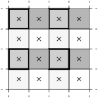
Figure 7: The four subgrids for plaquette changes, each shaded differently.

5.3 Results and Comparison

We have investigated the three different baby Skyrme models mentioned before. To that end, we need to minimize the energy functional:

$$E\left[\vec{\phi}\right]=\int\!\mathrm{d}^{2}x\left[\frac{1}{2}\partial_{i}\vec{\phi}\cdot\partial_{i}\vec{\phi}+\theta_{S}\left[(\partial_{i}\vec{\phi}\cdot\partial_{i}\vec{\phi})^{2}-(\partial_{i}\vec{\phi}\cdot\partial_{j}\vec{\phi})(\partial_{i}\vec{\phi}\cdot\partial_{j}\vec{\phi})\right]+\theta_{V}V(\vec{\phi})\right].$$ (36)

First, we have looked at the simplest holomorphic model with the potential $V=(1+\phi_{3})^{4}$. There exists an explicit 1-soliton solution,

$$W=\sqrt[4]{\frac{\theta_{V}}{2\theta_{S}}}~{}(x+\mathrm{i}y),$$ (37)

where the $W$ field is the stereographic projection of $\vec{\phi}$ on the complex plane, given by $W=2(\phi_{1}+\mathrm{i}\phi_{2}){(1-\phi_{3})}^{-1}$. We choose $\theta_{S}=\theta_{V}=\frac{1}{2}$ where its total energy equals $4\pi(1+\frac{8}{3\sqrt{2}})\approx 36.2618$. Since the soliton profile has a polynomial decay, we need a large lattice. With a $350\times 350$ grid and lattice spacing $h=0.05$, we obtain $E=36.4890$ and $B=0.9999$. Here, the energy is slightly higher than the exact solution because of the finite lattice effects. The holomorphic baby skyrmion has the slowest decay of any of the models discussed, and therefore can be seen as the worst case scenario.

	1-vacuum model			2-vacua model
Topological	SA		Ref. [12]	SA		Ref. [12]
Charge	$B$	$E/B$	$E/B$	$B$	$E/B$	$E/B$
1	0.99978	19.6505	19.47	0.99989	19.6572	19.65
2	1.99973	18.4452	18.27	1.99984	17.6530	17.65
3	2.99962	18.5257	18.34	2.99983	17.2259	17.22
4	3.99952	18.4014	18.22	3.99989	17.0677	17.07

Table 2: Baby Skyrme models: Comparison of our SA results with Euler-Lagrange results.

We have also looked at the baby Skyrme models with one vacuum, where $V=1+\phi_{3}$, and two vacua, where $V=1-\phi_{3}{}^{2}$. The parameters for the 1-vacuum model have been fixed to $\theta_{S}=\frac{1}{4}$ and $\theta_{V}=0.1$ and for the 2-vacua to $\theta_{S}=0.44365$ and $\theta_{V}=0.05$ in agreement with existing literature, see Ref. [12]. We use an $80\times 80$ grid with periodic boundary conditions and lattice spacing $h=0.4$. The minimal energy solution in the first four topological sectors is shown in Fig. 8 and Fig. 9 respectively. We compare the energies per charge with the calculations from Ref. [12] in Table 2.

The results for the 2-vacua model are the same for both studies within an accuracy of a few parts in $10^{4}$. The results from Ref. [12] have been obtained via the shooting method. We can apply this accurate method, because the skyrmions are radially symmetric and the minimization reduces to a 1D problem. There is a slight discrepancy in energy when comparing the 1-vacuum model. The energies in Ref. [12] were obtained on a 2D lattice using a damped time-evolution. The energy of the 1-skyrmion calculated using the shooting method is $E=19.65$. Our SA result agrees well with this value. The inaccuracies in Ref. [12] arise due to a different derivative approximation, which tends to reduce the energy. The errors due to the fixed boundaries are also greater in Ref. [12], although this tends to increase the energy of the 1-skyrmion. We believe that periodic boundary conditions, which have been used for our SA result, have the advantage that the tails of the skyrmions can spread out further. The finite lattice effects are still present, as skyrmions could then interact with themselves over the boundaries. For our SA model, a study [8] on the 1-skyrmion case shows that the gridsize used induces an error of the order 0.01%. The error due to not having relaxed the system properly is 0.01%. The largest error is due to finite difference effects and has a possible error of 0.1%. Because of the successful agreement of our SA result for the 1-skyrmion with the result of the shooting method, it is believed that the SA solutions with higher topological charge are also more accurate than the results quoted in Ref. [12]. Finally, we show shows an example of the cooling schedule for its 3-skyrmion in Fig. 10.

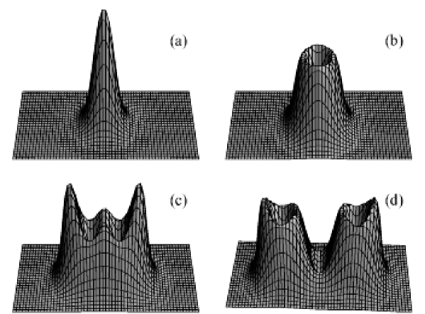
Figure 8: Energy density plot with identical vertical energy scale. We show the 1-vacuum skyrmions of charge one (a), two (b), three (c) and four (d). The range plotted is $2.4\times 1.2$ units in each figure.

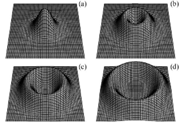
Figure 9: Energy density plot with identical vertical energy scale. We show the 2-vacua skyrmions of charge one (a), two (b), three (c) and four (d). The range plotted is $2.0\times 1.0$ units in each figure.

We studied three different baby Skyrme models. Changing from one potential to the other could not have been easier. In the case of the iterative techniques, changing the differential equation is in itself conceptually easy, but, in practice, a lot of time is spent on getting the coefficients right and checking the derivation. For future research, we intend to use SA to do a systematic check on the multi-skyrmion structure. Specifically, we are interested in the class of potentials that leads to radially symmetric multi-skyrmions.

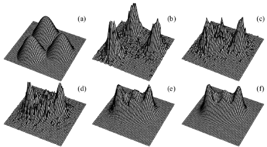
Figure 10: Energy density plot of identical vertical energy scale. We show a SA cooling for the 3-skyrmion in the 1-vacuum model: (a) the starting configuration; (b) system is heated to $\beta=500$ and skyrmions repel each other because their isospins are initially in the same direction; (c) isospins rotate relative to each other and skyrmions attract each other; (d) equilibrium has been reached for $\beta=500$; (e) system is cooled to $\beta=5000$; (f) minimal energy solution at $\beta=\infty$. The range plotted is $1.8\times 1.6$ units in each figure.

6 Simulated Annealing in 3D

We have chosen the nuclear Skyrme model [5] for our 3D SA implementation, because we believe that SA is a flexible tool for exploring the multi-skyrmion structure.

In the sixties, Skyrme constructed an effective field theory of mesons where the baryons are the topological solitons of the theory. Research by ’t Hooft and Witten has established that the nuclear Skyrme model shows important similarities to the low-energy effective lagrangian of QCD [27, 28]. The 1-skyrmion can be interpreted as a nucleon with reasonable success [29]. The numerical work by Braaten, Townend, and Carson [30], and Battye and Sutcliffe [31] on the structure of classical multi-skyrmions supports the idea that an appropriate quantization of these minimal energy solutions for a given topological sector could possibly lead to an effective description of atomic nuclei. However, the calculation of quantum properties of multi-skyrmions is very difficult. Part of this is due to the fact that these minimal energy solutions are not radially symmetric and the theory is non-renormalisable. This is rather frustrating, for the claim that the Skyrme model, descending from a large $N$-QCD approximation models mesons, baryons and higher nuclei is a very attractive one. Numerical methods are probably the only way forward and the SA scheme might be useful in exploring further the multi-skyrmion structure for different versions of the Skyrme model.

6.1 The Nuclear Skyrme Model

The nuclear Skyrme lagrangian

$$\mathcal{L}=\frac{1}{2}\partial_{\mu}\vec{\phi}\cdot\partial^{\mu}\vec{\phi}-\frac{1}{4}\left[(\partial_{\mu}\vec{\phi}\cdot\partial^{\mu}\vec{\phi})^{2}-(\partial_{\mu}\vec{\phi}\cdot\partial_{\nu}\vec{\phi})(\partial^{\mu}\vec{\phi}\cdot\partial^{\nu}\vec{\phi})\right]$$ (38)

is a straightforward extension of the nonlinear $\sigma$ model containing an additional fourth-order term called the Skyrme term. We need to include this extra term to ensure stability of the soliton. The mapping becomes

$$\phi(t):\mathrm{S}^{3}\longrightarrow\mathrm{S}^{3}.$$ (39)

More realistic lagrangians should probably include higher order correction terms. The SA scheme is especially useful, because extra term can be included trivially.

6.2 Implementation

The 3D implementation is very similar to the 2D code and we will only mention new issues relevant to the 3D case. On a 4D unit sphere, the integration measure is given by

$$\int_{\rm unit~{}sphere}\!\mathrm{d}x~{}\mathrm{d}y~{}\mathrm{d}z~{}\mathrm{d}w = \int_{\theta=0}^{2\pi}\int_{\phi=0}^{\pi}\int_{\chi=0}^{\pi}\!\sin\theta\sin^{2}\chi~{}\mathrm{d}\phi~{}\mathrm{d}\theta~{}\mathrm{d}\chi$$ (40)

$$= \int_{\theta=0}^{2\pi}\int_{\cos\theta=-1}^{1}\int_{\frac{\chi}{2}-\frac{1}{4}\sin(2\chi)=0}^{\frac{\pi}{2}}\!\mathrm{d}\phi~{}\mathrm{d}\cos\theta~{}\mathrm{d}\left(\frac{\chi}{2}-\frac{1}{4}\sin(2\chi)\right)$$

$$= \int_{\theta=0}^{2\pi}\int_{u=-1}^{1}\int_{v=0}^{\frac{\pi}{2}}\!\mathrm{d}\theta~{}\mathrm{d}u~{}\mathrm{d}v.$$

In order to rotate the new vector from the intrinsic frame to the laboratory frame, the angle $\chi$ must be evaluated from $v$. The equation

$$v=\frac{\chi}{2}-\frac{1}{4}\sin(2\chi)$$ (41)

can not be rewritten in terms of $\chi$, and therefore it must be solved numerically. The observation that most solutions will be in the region of small $v$ due to the importance sampling, implies that a small $\chi$ approximation might be useful. For small $\chi$, $v\approx\frac{\chi^{3}}{3}$. Therefore, the inversion is performed numerically by tabulating $\chi$ uniformly on $[0,\pi]$ against $v^{1/3}=\left(\frac{\chi}{2}-\frac{1}{4}\sin(2\chi)\right)^{\frac{1}{3}}$. The $\chi$ value corresponding to the selected $v^{\frac{1}{3}}$ is found in this table, and a linear interpolation is applied between the two nearest values of $v^{\frac{1}{3}}$ to give a better approximation to $\chi$. Using 1000 pre-calculated entries the error on the whole region $\chi\in[0,\pi]$ is then less than $10^{-7}$. On the region $\chi\in[0,0.1]$, where almost the entire selection of $\chi$ lies, the error is less than $10^{-14}$, which corresponds to the precision of double real numbers. This method does not create any significant errors and is time-consuming. No faster method seems to be possible.

As the cosines and sines of $\phi$, $\theta$, and $\chi$ are known, the rotation can be performed using a rotation matrix similar to (33). The new choice of vector in the intrinsic frame is given by

$$\vec{n}^{\rm int}=(n_{1}^{\rm int},n_{2}^{\rm int},n_{3}^{\rm int},n_{4}^{\rm int})=(\sin\chi\sin\theta\cos\phi,\sin\chi\sin\theta\sin\phi,\sin\chi\cos\theta,\cos\chi).$$ (42)

The $z$-axis in the intrinsic frame coincides with $\vec{k}^{\rm lab}=\vec{\phi}_{\rm present}(x_{k})$ in the laboratory frame, similarly as in the baby Skyrme model. The rotation angles $\gamma$, $\alpha$, and $\beta$ (in that order) are defined by

$$\vec{k}^{\rm lab}=(\cos\beta\sin\alpha\sin\gamma,\sin\beta\sin\alpha\sin\gamma,\cos\alpha\sin\gamma,\cos\gamma).$$ (43)

The transformation $\vec{n}^{\rm int}$ to $\vec{n}^{\rm lab}$ is performed using the matrix

$$\left(\begin{array}[]{c}n_{1}^{\rm lab}\\ n_{2}^{\rm lab}\\ n_{3}^{\rm lab}\\ n_{4}^{\rm lab}\end{array}\right)=\left(\begin{array}[]{cccc}\cos\alpha\cos\beta&-\sin\beta&\sin\alpha\cos\beta\cos\gamma&\sin\alpha\cos\beta\sin\gamma\\ \cos\alpha\sin\beta&\cos\beta&\sin\alpha\sin\beta\cos\gamma&\sin\alpha\sin\beta\sin\gamma\\ -\sin\alpha&0&\cos\alpha\cos\gamma&\cos\alpha\sin\gamma\\ 0&0&-\sin\gamma&\cos\gamma\end{array}\right)\left(\begin{array}[]{c}n_{1}^{\rm int}\\ n_{2}^{\rm int}\\ n_{3}^{\rm int}\\ n_{4}^{\rm int}\end{array}\right).$$ (44)

For similar reasons as already discussed previously, we use a restricted transition probability to be uniform over $[0,A)$, where $A\leq\pi$. The method of importance sampling has also been investigated for the nuclear Skyrme model and is given in the appendix. The transition probability is therefore

$$T(Y\mid X)=\left\{\begin{array}[]{cl}\frac{1}{4\pi A}&{\rm if}~{}\frac{\chi}{2}-\frac{1}{4}\sin(2\chi)<A\\ 0&{\rm otherwise.}\end{array}\right.$$ (45)

The angles are sampled by

$$v = \frac{\chi}{2}-\frac{1}{2}\sin(2\chi)=A\xi_{1},$$

$$u = \cos\theta=2\xi_{2}-1,$$

$$\phi = 2\pi\xi_{3},$$ (46)

where $\xi_{1}$, $\xi_{2}$ and $\xi_{3}$ are three random variables uniformly sampled from 0 to 1. The new vector $\vec{\phi}_{n}(x_{k})=\vec{n}^{\rm lab}$ is a vector which has been selected from a uniform probability distribution centered around the previous vector $\vec{\phi}_{p}(x_{k})~{}(=\vec{k}^{\rm lab})$ where only the angle $\chi$ between these vectors has an upper limit. Finally, $\vec{\phi}_{n}(x_{k})$ and $\vec{\phi}_{p}(x_{k})$ are inserted into (30) to find the acceptance rate. Similarly to the baby Skyrme models, the value of $A$ is automatically chosen to have an acceptance rate near 40%. The cooling is also controlled in the same manner as described in 2D.

6.3 Results and Comparison

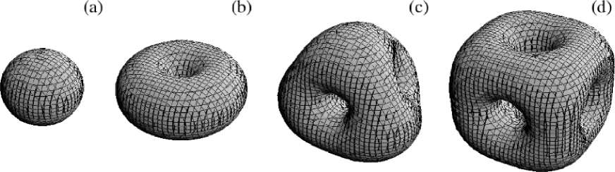
Figure 11: Plot of the same constant energy density surface. We show the first four multi-skyrmion solutions (from left to right). All plots are to the same scale. The mesh spacing of the plotted objects is 0.12 units.

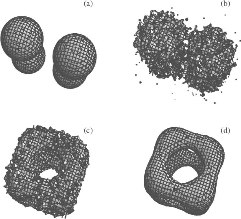
Figure 12: Plot of constant energy density surface. We show a SA search of the $B=4$ skyrmion: (a) the starting configuration of four 1-skyrmions; (b) the system heated to $\beta=500$ where the skyrmions fuse into one; (c) the system in equilibrium at $\beta=500$ where the structure emerges; (d) the minimal energy solution at $\beta=\infty$. All plots are to the same scale. The mesh spacing of the plotted objects is 0.1 units.

The 3D implementation of SA is computationally much more intensive than the 2D case. The accuracy of our numerical simulations is therefore reduced due to limited resources in computation time and memory. The intergrid spacing used is 0.12 Skyrme units and is close to the upper limit where the numerics break down (at a reasonably high temperature required to do SA sufficiently fast). The maximum gridsize that can be used to obtain results in a reasonable time is $80\times 80\times 80$. The finite volume causes an increase of energy for the 1-skyrmion because it repels itself over the periodic boundary, and therefore induces an error of 1% [8]. The error due to not having relaxed the system properly is 0.1%. The error due to finite difference effects has a maximum of 0.3%. The skyrmions of topological charge one to four are shown in Fig. 11. We show an an example of the cooling schedule for the 4-skyrmion in Fig. 12. These energies per charge are contrasted in table 3 with those results obtained by Battye and Sutcliffe [31]. It is very difficult to compare the results. The 1-skyrmion solution gives more information for comparison. It is spherically symmetric and the shooting method in the hedgehog ansatz can be used. The energy of a 1-skyrmion minimized in the 1D SA code is $E=73.12$ (in the continuous limit). We are not sure if the result for the 1-skyrmion in Ref. [31] is truly more accurate or just a coincidence. Their topological charge, an indicator for the discretization error, is certainly less accurate. The finite lattice effect increases the energy of the 1-skyrmion and therefore the energy obtained should be larger than 73.12. Unfortunately, we do not know which lattice parameters they have used, making a good comparison impossible. However, we get the same minimal energy structure.

Topological	SA		Ref. [31]
Charge	$B$	$E/B$	B	$E/B$
1	1.0015	73.75	0.984	72.96
2	2.0030	70.31	1.972	69.34
3	3.0042	68.52	2.960	67.69
4	4.0048	66.30	3.948	66.09

Table 3: The nuclear Skyrme model: SA results versus published results.

7 Conclusion

We have shown that SA is an alternative way of finding the minimal energy solution in a given topological charge sector. We independently confirmed the validity of the studies using the standard minimization techniques. It is very hard to objectively compare the different approaches. However, we have found SA to be a more convenient and flexible minimization technique. The implementation and fine-tuning of our SA codes took a fair amount of time due to a lack of prior research in this area. In comparison to other methods, we are confident that future implementations will take us considerably less time. We did not find any significant differences in speed of minimization. The SA codes can be made faster by fine-tuning the cooling parameters. We prefer SA minimization because of its ease of use. Speed considerations are irrelevant in 1D and 2D and we can use parallel computing in the 3D case. There are several areas we want to look at next. First of all, we will optimize SA by using more sophisticated update and cooling mechanisms and by parallelization. We are also currently investigating the possibility of doing time-evolution via SA minimization of the action. At the same time, we intend to look at a wide range of models. We shall investigate the multi-skyrmion structure of several baby Skyrme models. Research is also underway in the use of symmetry breaking terms for the nuclear Skyrme model. Moreover, the 2D and 3D code will be used to study phase transitions in the baby and nuclear Skyrme model at finite temperatures and finite densities [23]. To conclude, SA is a flexible tool; all we really need is an energy functional to minimize!

References

- [1] J. S. Russell, Rep. 14th Meet. BAAS, York (John Murray, London, 1844), p. 311.
- [2] P. G. Drazin and R. S. Johnson, Solitons: an introduction (Cambridge University Press, Cambridge, UK, 1996).
- [3] L. H. Ryder, Quantum Field Theory (Cambridge University Press, Cambridge, UK, 1994), chapter 10.
- [4] S. L. Sondhi, A. Karlhede, S. A. Kivelson, and E. H. Rezayi, Phys. Rev. B 47, 16419 (1993).
- [5] G. Holzwarth and B. Schwesinger, Rep. Prog. Phys. 49, 825 (1986).
- [6] A. Vilenkin and E. P. S. Shellard, Cosmic strings and other topological defects (Cambridge University Press, Cambridge, UK, 1994).
- [7] M. Duff, hep-th/9805177 (unpublished).
- [8] O. Schwindt, internal UMIST report (unpublished).
- [9] T. Weidig, Ph.D. thesis, University of Durham, 1999.
- [10] L. Ingber, J. Math. Comp. Model. 18, 29 (1993).
- [11] W. H. Press, S. A. Teukolsky, W. T. Vetterling, and B. P. Flannery, Numerical recipes in C (Cambridge University Press, Cambridge, UK, 1992).
- [12] T. Weidig, Nonlinearity 12, 1489 (1999).
- [13] N. Metropolis, A. W. Rosenbluth, M. N. Rosenbluth, and A. H. Teller, J. Chem. Phys. 21, 1087 (1953).
- [14] M. H. Kalos and P. A. Whitlock, Monte Carlo Methods (John Wiley, New York, 1986).
- [15] S. Kirkpatrick, C. D. Gelatt, and M. P. Vecchi, Science 220, 671 (1983).
- [16] S. Geman and D. Geman, IEEE Trans. Patt. Anal. Mac. Int. 26, 721 (1984).
- [17] R. Rajarman, Solitons and instantons (North-Holland, Amsterdam, 1996).
- [18] S. Coleman, Phys. Rev. D 11, 2088 (1975).
- [19] D. Vanderbilt and S. G. Louie, J. Comput. Phys. 56, 259 (1984).
- [20] G. H. Derrick, J. Math. Phys. 5, 1252 (1964).
- [21] B. M. A. G. Piette and W. J. Zakrzewski, Chaos, Solitons and Fractals 5, 2495 (1995).
- [22] B. M. A. G. Piette, B. J. Schoers, and W. J. Zakrzewski, Z. Phys. C 65, 165 (1995).
- [23] O. Schwindt and N. Walet (unpublished).
- [24] F. Mandel, Statistical physics (John Wiley, New York, 1988).
- [25] K. Binder, Monte Carlo Methods (Springer-Verlag, Berlin, 1979).
- [26] D. Frenkel and B. Smith, Understanding Molecular Simulation (Academic Press, London, 1996).
- [27] G. ’t Hooft, Nucl. Phys. B 72, 461 (1973).
- [28] E. Witten, Nucl. Phys. B 160, 55 (1979).
- [29] G. Adkins, C. Nappi, and E. Witten, Nucl. Phys. B 228, 552 (1983).
- [30] E. Braaten, S. Townend, and L. Carson, Phys. Lett. B 235, 147 (1990).
- [31] R. A. Battye and P. M. Sutcliffe, Phys. Rev. Lett. 79, 363 (1997).