UPR-875-T

CALT-68-2262

CITUSC/00-009

hep-th/0002057

Infra-red fixed points at the boundary

Klaus Behrndt^a and  Mirjam Cvetič^b

^a California Institute of Technology

Pasadena, CA 91125

CIT-USC Center For Theoretical Physics

University of Southern California

Los Angeles, CA 90089-2536

^b Department of Physics and Astronomy

University of Pennsylvania, Philadelphia, PA 19104-6396

Abstract

Gauged supergravities (in four and five dimensions) with eight supercharges and with vector supermultiplets have a unique ultra-violet (UV) fixed point on a given physical domain ${\cal M}$ of the space of the scalar fields. We show that in these models the infra-red (IR) fixed points are located on the boundary of ${\cal M}$, where the space-time metric becomes singular.

Over the past year a lot of attention has been given to elucidate, via AdS/CFT correspondence, the renormalization group (RG) flow of strongly coupled gauge theory in terms of static domain wall solutions in anti-deSitter (AdS) supergravity theories [1, 2, 3, 4]. In particular, the kink solutions of scalar-fields interpolating between the (supersymmetric AdS) extrema of gauged supergravity potentials provide a frame-work to address the aspects of RG flows on the dual gauge theory. (The first examples of supersymmetric domain wall solutions was found in the context of D=4 N=1 supergravity theory [5] and reviewed in [6].)

In gauged supergravity theories the scalar potential is of a restricted type, in particular, most of the supersymmetric extrema are maxima of the potential and thus in general it is difficult to obtain scalar kink solutions which at short space-time distances asymptote to the Cauchy horizon of the AdS space-time and which would correspond to infra-red (IR) fixed points. For this latter type of behavior in the IR the potential exhibits the second supersymmetric extremum, which is a saddle point or a minimum. Nevertheless an example of this type has been discussed in [2] for non-Abelian gauged supergravity, associated with the massless supermultiplets of Type IIB supergravity compactified on a five-sphere $S^{5}$ (D=5 N=8 gauged supergravity). In [7] another example of this type is due to the scalars of a massive supermultiplet of sphere reductions – those are breathing modes parameterizing the volume of the internal sphere.

In general, the maximally supersymmetric extremum of gauged supergravity potentials, which is always a maximum, is responsible for the kink solutions that asymptote at large distances (the ultra-violet (UV) fixed point) to the boundary of the AdS space-time, i.e. the corresponding conformal field theory in the UV is specified at the boundary of AdS space-time. On the other hand, the flows from this UV fixed point generically exhibit a singularity in the IR, i.e. the kink solution approaches at short distances the values of the run-away potential. For such examples within D=5 N=8 gauged supergravity see, e.g., [8, 9].

These latter features of the RG flows seem to be more generic within a set-up of gauged supergravity theories. For N=2 D=5 gauged supergravity with vector supermultiplets only, it has been shown [8, 9] that the potential has only a single extremum for any physical domain ${\cal M}$ of the moduli space for the scalar fields ($\phi_{A}$) and this extremum corresponds to an UV fixed point, where the space-time asymptotes to the AdS boundary. The same holds [9] for N=2 D=4 gauged supergravity with vector supermultiplets, only. On the other hand the kink solution at small distances (in the IR regime) necessarily reaches the singular domain at the boundary of $\cal M$, where both the scalar potential and the space-time become singular. Flows into such singular regions have been also discussed in [10, 11, 12].

The purpose of this letter is to show that, in spite of the singular nature at the boundary of ${\cal M}$, the solutions always exhibit an IR fixed point there, i.e. the $\beta$ functions vanish there ($\beta^{A}\Big{|}_{0}=0$) and their first derivatives $\partial_{A}\beta^{B}(\phi)\Big{|}_{0}$ are positive definite. The ordinary space-time (in D=4,5) also becomes singular at this (small) distance. However, the geodesic distance on ${\cal M}$, is infinite. To reiterate, these results hold for D=5 and D=4 gauged supergravity with eight supercharges and with vector supermultiplets, only. In D=4, the results change [6, 5] if one allows for only four unbroken supercharges.

Let us start with some general remarks. In order to get a proper RG flow interpretation of the supergravity we have to choose a specific coordinate system for the space-time metric [13, 3, 14]:

$$ds^{2}=u^{2}\Big{(}-dt^{2}+d\vec{x}^{2}\Big{)}+{du^{2}\over W(u)^{2}u^{2}},$$ (1)

where $W(u)^{2}$ becomes the cosmological constant or inverse AdS radius at the UV fixed point ($u\rightarrow\infty$), however, for a finite $u$, it varies. The IR region corresponds to $u\rightarrow 0$. Using this coordinate system, the solution preserves supersymmetry if the scalar fields satisfy the following equation [3, 14]:

$$\beta^{A}\equiv u{d\over du}\phi^{A}=g^{AB}\partial_{B}\log|W|^{-(D-2)}=g^{AB}\partial_{B}\log C,$$ (2)

where $\phi^{A}$ are the scalar fields and the second equation is a proposal [1, 2, 3] for the definition of the $C$-function. The quantities $W$ and $g_{AB}$ , that enter the metric (1) and the $\beta^{A}$ functions (2), are nothing but the superpotential and the metric of the scalar fields $\phi^{A}$ whose Lagrangian reads

$$S_{D}=\int d^{D}x\ \Big{[}{\frac{1}{2}}R-V-{\frac{1}{2}}g_{AB}\partial_{\mu}\phi^{A}\partial^{\mu}\phi^{B}\Big{]},$$ (3)

and the potential has the form

$$V=2(D-2)(D-1)\,\Big{(}\,{D-2\over D-1}g^{AB}\partial_{A}W\partial_{B}W-W^{2}\,\Big{)}\ .$$ (4)

Obviously, at extrema of $W$ the $\beta^{A}$ functions (2) vanish and we reach an AdS space. In general, the constraints of gauged supergravity impose constraints on the form of $W$. Thus only very specific solutions of the RG flows can take place.

Let us focus on D=5 case, first. D=5 gauged supergravity with eight supercharges and the vector super-multiplets, whose scalars $\phi^{A}$ parameterize a hypersurface ${\cal M}$, are defined by a cubic equation [17]:

$$F(X)\equiv{1\over 6}\,C_{IJK}X^{I}X^{J}X^{K}=1,$$ (5)

where $I=0,1,2,\ldots n$ and $n$ is the number of auxiliary vector supermultiplets $X^{I}$ and $C_{IJK}$ are the coefficient defining the cubic Chern-Simons term in the supergravity Lagrangian. In Calabi-Yau compactifications these are the topological intersection numbers and the constraint (5) means that the volume is kept fix. In general ${\cal M}$ is not connected and consists of different branches, separated by regions where $F(X)<0$; see figure 1.

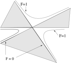
Figure 1: The scalar fields of vector super-multiplets of D=5 theory parameterize a manifold that consists of different branches. The straight lines correspond to F=0 domain and shaded areas to $F<0$ domains.

The potential is generated by gauging a $U(1)$ subgroup of the $SU(2)$ R-symmetry [18] and the superpotential $W$ and the scalar metric have the form

$$W=\alpha_{I}X^{I}\qquad,\qquad\ g_{AB}=-{1\over 2}\Big{(}\partial_{A}X^{I}\partial_{B}X^{J}\,\partial_{I}\partial_{J}\log F(X)\Big{)}\Big{|}_{F=1}\ ,$$ (6)

where $\alpha_{I}$ are constant parameters of the $U(1)$ gauging. Using general formulae from [17], one can expand $W$ around a critical point ($\partial_{A}W=0$) and one finds

$${W\over W_{0}}=1+{1\over 3}g_{AB}(\phi^{A}-\phi^{A}_{0})(\phi^{B}-\phi_{0}^{B})+...$$ (7)

Inserting this expression into the $\beta$-function (2) one gets [3]

$$\beta^{A}=-2(\phi^{A}-\phi_{0}^{A})+{\cal O}(\Delta\phi^{2}),$$ (8)

and consequently $\partial_{B}\beta^{A}=-2\,\delta_{B}^{\ A}$, which means that extrema of $W$ are UV fixed points [8]. In fact the sign in front of the second term in the expansion (7) determines the nature of the fixed point; for positive values it is an UV and for negative an IR fixed point. Since there is only one extremum of $W$ per nonsingular physical domain of $\cal M$ [9] , one concludes that this extremum always corresponds to the UV fixed point. Equivalently, space-time asymptotes to the AdS boundary there [8, 9].

Having this UV fixed point, let us now discuss the domain near the boundary of ${\cal M}$, which is defined by zeros of $F(X)$. For the discussion, it is convenient to use projective coordinates, i.e. to define the physical scalars as $\phi^{A}=X^{A}/X^{0}$ and $F(X)$ and the superpotential becomes

$$F=(X^{0})^{3}p_{3}(\phi),\qquad W=X^{0}\Big{(}\alpha_{0}+\alpha_{A}\phi^{A}\Big{)},$$ (9)

where $p_{3}(\phi)$ is a polynomial of third degree in $\phi^{A}$. For the single scalar case, e.g., we obtain $p_{3}(\phi)=(\phi-\phi_{1})(\phi-\phi_{2})(\phi-\phi_{3})$ and reach the boundary of ${\cal M}$ at zeros of this polynomial, i.e. at $\phi=\phi_{1,2,3}$. Due to the requirement of $F=1$ the zeros of $p_{3}(\phi)$ translate into poles of $X^{0}$ and therefore into poles of $W$. There are two cases to distinguish, if $p_{3}(\phi)$ has a single ($n=1$) or double ($n=2$) zero. Note the case $\phi_{1}=\phi_{2}=\phi_{3}$ is trivial; there are no physical scalars. The situation for the multi-scalar case is analogous, i.e. we have either a linear or quadratic zero of $p_{3}$ (and the corresponding pole of $W$). Therefore, for generic values of $\alpha_{I}$ the superpotential behaves near the boundary as

$$W\sim\lambda^{-n/3},\ \ n=1,2,$$ (10)

where $\lambda\rightarrow 0$ denotes a scaling parameter in terms of the deviation of the scalars from their boundary value, e.g.,  for the single scalar case we can write $\lambda\equiv\phi-\phi_{0}$. Similarly, one obtains for the scaling of the metric

$$g_{AB}={1\over 3\lambda^{2}}\hat{g}_{AB}\ ,$$ (11)

where $\hat{g}_{AB}$ is the part which remains finite (and positive definite) on the boundary. Using these simple scaling arguments one obtains for the $\beta$ function near the boundary

$$\beta^{A}=3n\hat{g}^{AB}(\phi^{B}-\phi_{0}^{B}),\ \ n=1,2.$$ (12)

In the case where all $\beta$ functions vanish, we reach a fixed point of the RG flow and because $\partial_{B}\beta^{A}$ is positive definite, these are indeed IR fixed points. This result should be contrasted with examples where there is a regular UV fixed points in the bulk (with a non-singular AdS space-time); see (8).

Moreover, the leading order term of the $\beta$ function near the UV fixed point was universal. On the other hand the $\beta$ function near the boundary depends on $\hat{g}^{AB}$, and is thus model-dependent. In the following we consider a number of examples.

Single scalar case. Inserting the near-boundary value of $\lambda=\phi-\phi_{0}$, we obtain $\beta=3\,n\,c\,(\phi-\phi_{0})$ with some model-dependent positive $c$. As a solution for the scalar field $\phi$ and $W$ one obtains [20]

$$\phi-\phi_{0}\sim u^{3\,n\,c}\quad,\quad W\sim u^{-n^{2}\,c}.$$ (13)

For $c=1$ the metric can be written as

$$\begin{array}[]{ll}ds^{2}=(az-z_{0})^{2}\Big{(}-dt^{2}+d\vec{x}^{2}\Big{)}+dz^{2},&{\rm for:}\quad n=1,\\ ds^{2}=\sqrt{az-z_{0}}\Big{(}-dt^{2}+d\vec{x}^{2}\Big{)}+dz^{2},&{\rm for:}\quad n=2,\end{array}$$ (14)

where $a$ is basically an integration constant. In both cases the space-time metric is singular. The second case has been encountered also in [10, 11]. Since this singularity corresponds to the boundary of ${\cal M}$, it is an infinite geodesic distance away, i.e. $\int_{\phi=\phi_{0}}\sqrt{g_{\phi\phi}}\,d\phi=\infty$ (see also the example below), even though the affine parameter along this trajectory as measured by the space-time radius $z$ or $u$ remains finite. Moreover, the zeros of $F(X)$ are not really the “end of the world”, they rather separate different phases of the theory related to the different branches of ${\cal M}$ and the infinite geodesic distance may indicates that each branch is related to a different topology. From the field theory point of view the different branches are related to different sides of an IR fixed point.

In order to elucidate the implications of this singularity from the higher dimensional viewpoint one may try to adopt arguments as used in [21] to regulate the solution or techniques used to resolve conical singularities in Calabi-Yau compactifications . E.g., if we replace the flat world-volume in the case $n=1$ by an space of constant curvature $k$, i.e. a de Sitter space, the D=5 metric becomes flat iff $k=a^{2}$. On the other hand, examples with $n=2$ that arise in D=4,5 theories as sphere reductions of M/string-theory, e.g., STU model (discussed later) have a higher dimensional interpretation as distributions of positive tension branes (see e.g., [22, 12] and references therein), and thus from higher dimensional perspective do not seem to suffer from pathologies. Let us also mention that higher curvature corrections provide a natural cut-off for the volume of the internal space and may be used as a regulator, see [23]. However, one has to keep in mind that any curvature cut-off will also remove the IR fixed point! The $\beta$ functions vanish only on the singularity.

Let us further consider two other specific examples:
(i) $F=ST^{2}-b\,T^{3}$, which is a single scalar case,
(ii) $F=STU$, which has two scalars.

Case (i). Defining the physical scalar as $\phi={T\over S}$, which parameterizes the angle in figure 1, we reach the boundaries at $F=S^{3}\phi^{2}(1-b\,\phi)=0$, i.e. at $\phi\rightarrow 0,{1/b}$. The first case corresponds to a double zero ($n=2$) and the latter to a single zero ($n=1$). The inverse metric and the derivative of the superpotential $W=S+T=S(1+\phi)$ (taking $\alpha_{I}=(1,1)$) become

$$g_{\phi\phi}={1\over 3\,\phi^{2}(1-b\,\phi)^{2}}\quad,\quad{\partial_{\phi}W\over W}={(3b+1)\phi-2\over 3\phi(\phi+1)(1-b\,\phi)},$$ (15)

and therefore the $\beta$ function reads

$$\beta^{\phi}=-3\,{\phi(1-b\,\phi)\,\big{[}(3\,b+1)\,\phi-2\big{]}\over\phi+1}.$$ (16)

We find three fixed points

$$\phi_{UV}={2\over 3b+1}\quad,\quad\phi_{IR}=\{0\,,\,1/b\},$$ (17)

with $\partial_{\phi}\beta|_{UV}=-2$ and $\partial_{\phi}\beta|_{IR}=\{6,3/b^{2}\}$ for $\phi=\{0,1/b\}$, respectively; notice the different values for the two IR fixed points which were in general parameterized by the coefficient $c$ in (13). The $\beta$ function is shown in figure 2 and it behaves smoothly over all branches of ${\cal M}$.

Figure 2: This figure shows the $\beta$ function (16) for a single scalar with which has three fixed points: $\phi_{IR}=0,1/b$ and $\phi_{UV}=2/(3b+1)$. The IR fixed points lie on the boundary of ${\cal M}$.

Case (ii). In this case we take as physical scalars $(T,U)$ ($S=1/TU$) and for the superpotential we take again $\alpha_{I}=(1,1,1)$ or $W=1/TU+T+U$. We find for the $\beta$ functions

$$\beta^{T}={2T\Big{(}1-2T^{2}U+TU^{2}\Big{)}\over 1+T^{2}U+TU^{2}}\quad,\quad\beta^{U}={2U\Big{(}1-2TU^{2}+T^{2}U\Big{)}\over 1+T^{2}U+TU^{2}}\ .$$ (18)

There are only two fixed points:

$$\Big{(}T,U\Big{)}_{UV}=(1,1)\qquad,\qquad\Big{(}T,U\Big{)}_{IR}=(0,0),$$ (19)

with $\partial_{A}\beta^{B}\Big{|}_{UV}=-2\,\delta_{A}^{\ B}$ and $\partial_{A}\beta^{B}\Big{|}_{IR}=2\,\delta_{A}^{\ B}$. Therefore, only one point on the boundary of $\cal M$ is an IR fixed point. However, this is a very special example of the two-scalar case. If one modifies $F$, e.g.,  $F=STU\rightarrow STU-b\,U^{3}$, one can obtain more than one IR fixed point.

We now comment also on D=4 gauged supergravity with eight supercharges. In this case, we have to replace the coordinates $X^{I}$ by the symplectic section $(X^{I},F_{I})$ where $F_{I}=\partial_{I}F(X)$ denotes the derivative of the prepotential. Using this symplectic section, a real superpotential can be defined by

$$\widehat{W}\equiv{1\over 2}\,\xi\,|We^{K/2}|={1\over 2}\,\xi\,|\alpha_{I}X^{I}-\beta^{I}F_{I}|e^{K/2}\ ,$$ (20)

with $W$ and $K$ as Super- and Kähler potential, respectively and $\xi=\pm 1$ (it can change sign iff $W$ crosses zero). In our notation the Kähler metric is defined as $g_{A\bar{B}}={1\over 2}\partial_{A}\partial_{\bar{B}}K$. Again, extrema of $\widehat{W}$ correspond to UV fixed points [9]. (For notation and conventions, see [24].) Here let us turn to the investigation of the boundary behavior of the RG equations.

In D=5 case one had to look at poles in $X^{0}$, see eq. (9). In D=4 these singularities are equivalent to poles in $e^{K/2}$. Taking a generic flux vector $(\alpha_{I},\beta^{I})$ the $\beta$ functions near such poles take the form:

$$\beta^{A}=-g^{A\bar{B}}(\partial_{\bar{B}}K+{\rm finite\ term})\ .$$ (21)

As before, we can use general scaling arguments to verify the behavior: $e^{-K}\sim\lambda^{n}$ and $g_{A\bar{B}}\sim{n\over 2}\lambda^{-2}$, where $n$ is again the degree of the pole with $n=1,2$.

An equivalent relation to (12) for the behavior near the pole $(z^{A}-z^{A}_{0})\simeq 0$ takes the form:

$$\beta^{A}=2\,\bar{g}^{A\bar{B}}(z^{B}-z_{0}^{B})\ ,$$ (22)

where $z^{B}={X^{B}\over X^{0}}$ is the complex scalar. Because the derivatives of these $\beta$ functions are positive definite we again obtain the IR fixed points at $z^{A}\simeq z_{0}^{A}$.

As an example, let us consider again the single-scalar case given by the prepotential $F=X^{0}X^{1}$, which yields the Kähler potential $e^{-K}=-i(T-\bar{T})$. In this case the $\beta$ function near the zero of $e^{-K}$ becomes

$$\beta(T)=2(T-\bar{T})\ ,$$ (23)

and therefore one reaches an IR fixed point at: Re$T=const.$, Im$T=0$. As for the UV fixed point, with the choice $(\alpha_{I},\beta^{I})=(1,1,0,0)$, one find the extremum of $\widehat{W}=|1-i\,T|e^{K/2}$ at Re$T=0$, Im$T=1$; near this point the $\beta$ function is of the form:

$$\beta(T)=-2(T-i)\ ,$$ (24)

with its first derivative negative and thus identified as a UV fixed point.

Acknowledgments

We would to thank H. Lü, D. Minić and H. Verlinde for useful discussions. M.C. would like to thank Caltech Theory Group for hospitality. The work is supported by a DFG Heisenberg grant (K.B.), in part by the Department of Energy under grant number DE-FG03-92-ER 40701 (K.B.), DOE-FG02-95ER40893 (M.C.) and the University of Pennsylvania Research Foundation (M.C).

References

- [1] L. Girardello, M. Petrini, M. Porrati, and A. Zaffaroni, “Novel local CFT and exact results on perturbations of N=4 super Yang-Mills from AdS dynamics,” JHEP 12 (1998) 022, hep-th/9810126.
- [2] D. Z. Freedman, S. S. Gubser, K. Pilch, and N. P. Warner, “Renormalization group flows from holography supersymmetry and a c-theorem,” hep-th/9904017.
- [3] K. Behrndt, “Domain walls of D = 5 supergravity and fixed points of N = 1 super Yang-Mills,” hep-th/9907070.
- [4] J. Distler and F. Zamora, “Non-supersymmetric conformal field theories from stable anti-de sitter spaces,” Adv. Theor. Math. Phys. 2 (1999) 1405, hep-th/9810206.
- [5] M. Cvetič, S. Griffies, and S.-J. Rey, “Static domain walls in N=1 supergravity,” Nucl. Phys. B381 (1992) 301–328, hep-th/9201007.
- [6] M. Cvetič and H. H. Soleng, “Supergravity domain walls,” Phys. Rept. 282 (1997) 159, hep-th/9604090.
- [7] M. Cvetič, H. Lu, and C. N. Pope, “Domain walls and massive gauged supergravity potentials,” hep-th/0001002.
- [8] R. Kallosh and A. Linde, “Supersymmetry and the brane world,” hep-th/0001071.
- [9] K. Behrndt and M. Cvetič, “Anti-deSitter vacua of gauged supergravities with 8 supercharges,” hep-th/0001159.
- [10] L. Girardello, M. Petrini, M. Porrati, and A. Zaffaroni, “Confinement and condensates without fine tuning in supergravity duals of gauge theories,” JHEP 05 (1999) 026, hep-th/9903026.
- [11] L. Girardello, M. Petrini, M. Porrati, and A. Zaffaroni, “The supergravity dual of N=1 super Yang-Mills theory,” hep-th/9909047.
- [12] N. P. Warner, “Renormalization group flows from five-dimensional supergravity,” hep-th/9911240.
- [13] A. W. Peet and J. Polchinski, “UV/IR relations in AdS dynamics,” Phys. Rev. D59 (1999) 065011, hep-th/9809022.
- [14] J. de Boer, E. Verlinde, and H. Verlinde, “On the holographic renormalization group,” hep-th/9912012.
- [15] P. K. Townsend, “Positive energy and the scalar potential in higher dimensional (super)gravity theories,” Phys. Lett. B148 (1984) 55.
- [16] K. Skenderis and P. K. Townsend, “Gravitational stability and renormalization-group flow,” Phys. Lett. B468 (1999) 46, hep-th/9909070.
- [17] M. Günaydin, G. Sierra, and P. K. Townsend, “The geometry of N=2 Maxwell-Einstein supergravity and Jordan algebras,” Nucl. Phys. B242 (1984) 244.
- [18] M. Günaydin, G. Sierra, and P. K. Townsend, “Gauging the D=5 Maxwell-Einstein supergravity theories: More on Jordan algebras,” Nucl. Phys. B253 (1985) 573.
- [19] M. Wijnholt and S. Zhukov, “On the uniqueness of black hole attractors,” hep-th/9912002.
- [20] K. Behrndt and M. Cvetič, “Supersymmetric domain wall world from D=5 simple gauged supergravity,” hep-th/9909058.
- [21] C. V. Johnson, A. W. Peet, and J. Polchinski, “Gauge theory and the excision of repulson singularities,” hep-th/9911161.
- [22] M. Cvetič, S. S. Gubser, H. Lu, and C. N. Pope, “Symmetric potentials of gauged supergravities in diverse dimensions and Coulomb branch of gauge theories,” hep-th/9909121.
- [23] K. Behrndt and S. Gukov, “Domain walls and superpotentials from M theory on Calabi-Yau three-folds,” hep-th/0001082.
- [24] D. Lüst, “String vacua with N = 2 supersymmetry in four dimensions,” hep-th/9803072; K. Behrndt, D. Lüst, and W. A. Sabra, “Stationary solutions of N = 2 supergravity,” Nucl. Phys. B510 (1998) 264, hep-th/9705169.