Vacuum Polarization and Energy Conditions at a Planar Frequency Dependent Dielectric to Vacuum Interface

Abstract

The form of the vacuum stress-tensor for the quantized scalar field at a dielectric-vacuum interface is studied. The dielectric is modeled to have an index of refraction that varies with frequency. We find that the stress-tensor components, derived from the mode function expansion of the Wightman function, are naturally regularized by the reflection and transmission coefficients of the mode at the boundary. Additionally, the divergence of the vacuum energy associated with a perfectly reflecting mirror is found to disappear for the dielectric mirror at the expense of introducing a new energy density near the surface which has the opposite sign. Thus the weak energy condition is always violated in some region of the spacetime. For the dielectric mirror, the mean vacuum energy density per unit plate area in a constant time hypersurface is always found to be positive (or zero) and the averaged weak energy condition is proven to hold for all observers with non-zero velocity along the normal direction to the boundary. Both results are found to be generic features of the vacuum stress-tensor and not necessarily dependent of the frequency dependence of the dielectric.

I Introduction

The renormalized vacuum stress-tensor for quantized fields at perfectly reflecting boundaries has been extensively studied, sufficiently so that they have made their way into various texts. Fulling [1] and Birrell and Davies [2] are two examples. The perfect reflector enforces a Dirichlet boundary condition that must be satisfied by the quantized field. For the case of the scalar or electromagnetic field with an infinite planar boundary, the renormalized vacuum energy density for stationary observers has the form

$$\langle\rho\rangle_{\mbox{Ren.}}={\alpha\over x^{m}},$$ (1)

where $\alpha$ is a unitless constant of order unity, $x$ is the transverse distance from the planar boundary and $m>1$ is the dimension of the spacetime. The most notable property of the energy density is the divergence in the limit $x\rightarrow 0$.

The divergence is not at all unexpected. The application of the Dirichlet boundary condition fixes the value of the field at a specific point with no uncertainty in the position. Thus the uncertainty of the conjugate momenta must be infinite, giving rise to the stress-tensor divergence. The precise mathematical origin of the divergence comes from the renormalization of the vacuum energy via the Green’s function. The argument is simply that the unrenormalized Green’s function is constructed such that it vanishes on the boundary. To renormalize the Green’s function, the corresponding Minkowski space Green’s function must be subtracted away. Since this is divergent in the limit $x\rightarrow 0$, the subtraction carried out for renormalization will leave behind a divergent part. When the vacuum energy is calculated from the renormalized Green’s function, it will diverge at $x=0$ also.

The divergence of the vacuum energy density causes considerable consternation since the vacuum would contain an infinite amount of energy. In a self consistent theory of gravity, the back reaction of the vacuum energy on the spacetime would be considerable. Yet we know from experience that metallic foils do not cause significant gravitational distortions around themselves.

There are three resolutions to the problems: (1) Replace the Dirichlet boundary condition with something more realistic, which is the topic of this paper. (2) Add position uncertainty to the mirror; this has been discussed by Ford and Svaiter [3]. (3) Treat the entire problem quantum mechanically, which has been partially touched upon by Barton and Eberlein [4] and more recently by Helfer [5].

Replacing the Dirichlet boundary condition has to some degree been discussed by other authors. For example Candelas [6] has derived the asymptotic form of the vacuum energy density for the problem of two nondispersive dielectric half-spaces which are in contact with one another along a planar interface. More recently Helfer and Lang [7] carried out similar calculations for a nondispersive dielectric to vacuum interface, with considerable interest placed upon the energy conditions in the vacuum region.

This paper addresses the behavior of the stress-tensor for a quantized massless scalar field at a planar dielectric to vacuum interface where the index of refraction of the material varies as a function of frequency. The Dirichlet boundary condition is replaced with appropriate frequency dependent reflection and transmission coefficients. The stress-tensor in the vacuum region is well behaved, even on the interface, and is largely independent of the functional dependence of the index of refraction. Therefore the vacuum energy divergence is a result of the Dirichlet boundary condition and not a generic feature of the field theory. It should be noted, however, that it is possible to get divergences for dielectric materials at the interface. The simplest example is a material with a constant index of refraction. In this case, the divergence comes about because part of the amplitude of the wave at every frequency still satisfies Dirichlet boundary conditions. The existence of the divergence is intimately tied to the failure of specific integrals to exist. For example, in two dimensions, a divergence will occur if

$$\int_{0}^{\infty}R(\omega)\,d\omega$$ (2)

fails to exist. Here $R(\omega)=\left[n(\omega)-1\right]/\left[n(\omega)+1\right]$ is the reflection coefficient for the modes at the interface, while $n(\omega)$ is the index of refraction. There are similar integrals in four dimensions involving both the reflection and transmission coefficients.

There are two remarkable results regarding frequency dependent dielectric models. First, all of the integrals that must be evaluated to find the components of the stress-tensor are self regularized, meaning that they all have a built in cutoff function that prevents ultraviolet divergences. For example, in two dimensions the energy density for a static observer is

$$\langle\rho\rangle_{\mbox{Ren.}}=-{2\xi\over\pi}\int_{0}^{\infty}\omega\,R(\omega)\,\cos(2\omega x)\,d\omega.$$ (3)

The only constraint placed on the index of refraction is for it to tend to unity as the frequency grows. Thus the reflection coefficient plays the role of the regulator in the integral. Similar results are found for the four-dimensional case as well, where there exists another integral for the evanescent modes which is regularized by the transmission coefficient.

The other unique property, which we shall prove in general, is that the vacuum stress-tensor satisfies the averaged weak energy condition (AWEC) for any moving geodesic observer, provided that the component of the observer’s four velocity normal to the dielectric to vacuum interface is non-zero. This occurs even though the pointwise weak energy condition (WEC) over some regions of the spacetime fails. The AWEC results from the Riemann-Lebesgue lemma applied to integrals of the form of Eq. (3) evaluated in the limit $x\rightarrow\infty$. In order to apply the lemma, it is required that conditions like (2) exist.

A related result is that the energy density, integrated along the normal direction in a constant time hypersurface in the vacuum region, is a positive constant. In two dimensions the constant is zero and independent of the choice of model for the index of refraction. Thus the spacetime always contains two regions, one where the vacuum energy is positive and another with equal negative energy. In four dimensions, the constant is found by evaluating the integral

$${E\over\mbox{unit area}}={1\over 64\pi}\int_{0}^{\infty}\omega^{2}\left[n^{2}(\omega)-1\right]d\omega$$ (4)

for a specific choice of $n(\omega)$. We consider only the class of models for which $n(\omega)\geq 1$ for all frequencies. The function space for which the integral holds is obviously much larger, however this is beyond the focus of this paper.

Specific models are examined in this paper. The vacuum stress-tensor is found to asymptotically approach the form of the perfectly reflecting vacuum stress-tensor in the large distance limit. The price of removing the divergence of the stress-tensor by using a frequency dependent dielectric is the introduction of a vacuum energy near the surface with opposite sign. This simultaneously is the reason why the AWEC holds while the WEC fails.

II Mode Structure at a Dielectric Interface

We begin with the source free scalar wave equation in m+1 dimensional Minkowski spacetime for a nondispersive material,

$$\left(\nabla^{2}-n^{2}\partial_{t}^{2}\right)\phi({\bf x},t)=0,$$ (5)

where $n$ is a constant. Units of $\hbar=c=1$ are being used throughout. A positive frequency plane wave solution to this equation in an infinite medium takes the form

$$f_{\bf k}({\bf x},t)\propto e^{i(n{\bf k}\cdot{\bf x}-\omega t)},$$ (6)

where $\omega=|{\bf k}|$. The modes can be normalized by defining the probability density for the wave equation and setting its integral over all space to unity. This leads to the normalization condition

$$\left(f_{\bf k}({\bf x},t),f_{\bf k^{\prime}}({\bf x},t)\right)\equiv-i\int d^{m}x\,n^{2}\left\{f_{\bf k}({\bf x},t)\left[\partial_{t}f_{\bf k^{\prime}}^{*}({\bf x},t)\right]-\left[\partial_{t}f_{\bf k}({\bf x},t)\right]f_{\bf k^{\prime}}^{*}({\bf x},t)\right\}=\delta^{m}({\bf k}-{\bf k^{\prime}}).$$ (7)

Thus the normalized plane wave mode takes the form

$$f_{\bf k}({\bf x},t)=n^{(m-2)/2}\,\left[2\omega(2\pi)^{m}\right]^{-1/2}e^{i(n{\bf k}\cdot{\bf x}-\omega t)}$$ (8)

The most general solution to the wave equation (5) is then given as a mode function expansion,

$$\phi({\bf x},t)=\int_{-\infty}^{+\infty}d^{m}k\left[a_{\bf k}f_{\bf k}({\bf x},t)+a_{\bf k}^{\dagger}f_{\bf k}^{*}({\bf x},t)\right].$$ (9)

If $\phi({\bf x},t)$ is a classical solution to the wave equation, then $a_{\bf k}$ and $a_{\bf k}^{\dagger}$ are the Fourier coefficients for the mode function expansion. The classical solution has the property that it can in general be written as

$$\phi({\bf x},t)=g(x-{1\over n}t)+h(x+{1\over n}t).$$ (10)

This represents two traveling waves, $g$ and $h$, that propagate in the $+\hat{x}$ and $-\hat{x}$ directions, respectively. Each traveling wave maintains a constant spatial profile that is just translated along the direction of motion. When second quantization is applied the coefficients $a_{\bf k}$ and $a_{\bf k}^{\dagger}$ become the annihilation and creation operators, respectively.

Next, consider wave propagation in a dispersive material. A scalar wave equation is needed which mimics the behavior of the electromagnetic field inside a dispersive material. In electromagnetism, the wave equation is found by first Fourier expanding the Maxwell equations for harmonic time dependence. Upon combining them, we find that each component of $\bf E$ and $\bf B$ must individually satisfy the Helmholtz wave equation

$$\left[\nabla^{2}-n^{2}(\omega)\omega^{2}\right]\phi({\bf x},\omega)=0.$$ (11)

We will take this to be our dispersive wave equation. The mode functions which satisfy this equation are the same as given above with the replacement $n\rightarrow n(\omega)$. The general solution $\phi({\bf x},t)$ is given as a mode function expansion in terms of the plane waves in the same form as (9). To obtain this form we must impose the condition $n^{*}(\omega)=n(\omega)$. However, even a simple resonance model (anomalous dispersion) for the dielectric as given in Jackson [8] leads to an index of refraction that does not satisfy this condition and would necessitate a more complicated quantum field theory. Thus, we restrict $n(\omega)$ to be real for simplicity. The physical interpretation of this condition is that the dielectric does not attenuate the wave propagating through it. It also excludes materials that may have any degree of conductivity. Strictly speaking, causality and the Kramers-Kronig relations require any index of refraction to have a nonzero imaginary part. However, it is also possible to have broad frequency bands within which the real part is very large compared to the imaginary part. Thus, for the models studied here, we are assuming that the dominant contribution to the energy density come from regions of the spectrum where $Re(n)\gg Im(n)$. The general solution to the wave equation in the time domain no longer has the physical property of traveling waves as in the nondispersive material. For this case, each frequency component propagates with a different velocity, so the overall profile of the wave changes as it moves.

Now consider the example of two different dielectrics which have a planar interface at $x_{1}=0$. To the left of the planar boundary the index of refraction will be denoted by $n_{I}$. To the right of the boundary the index will be $n_{T}$. In addition we will define the normal to the interface, $\hat{\bf u}=(1,0,\cdots,0)$. We allow a monochromatic plane wave to be incident on the interface from the left with a momentum ${\bf k}_{I}$. At the interface this incident wave is partly reflected back into the first medium and partly transmitted into the second medium. The reflected and transmitted waves have momenta ${\bf k}_{r}$ and ${\bf k}_{t}$ respectively, and the three components of the wave are

$$\phi_{inc.}({\bf x},t) = e^{i(n_{I}{\bf k}_{I}\cdot{\bf x}-\omega_{I}t)}$$ (12)

$$\phi_{refl.}({\bf x},t) = R\,e^{i(n_{I}{\bf k}_{R}\cdot{\bf x}-\omega_{R}t)}$$ (13)

$$\phi_{tran.}({\bf x},t) = T\,e^{i({\bf k}_{T}\cdot{\bf x}-\omega_{T}t)}$$ (14)

For electromagnetism, the plane wave modes at the boundary would have to satisfy the continuity of the transverse and perpendicular components of the fields across the interface. For the scalar field, the boundary conditions that will be applied are the continuity of $\phi({\bf x},t)$ and $\partial_{x}\phi({\bf x},t)$ across the boundary. This leads to several relations:

1. The continuity relations must hold at all times, therefore we must impose

   $$\omega_{I}=\omega_{R}=\omega_{T}=\omega.$$ (15)

2. All of the terms must have the same functional dependence on the surface of the interface, therefore

   $$n_{I}{\bf k}_{I}\cdot{\bf x}\,=\,n_{R}{\bf k}_{R}\cdot{\bf x}={\bf k}_{T}\cdot{\bf x}\;\;\mbox{at}\;x_{1}=0.$$ (16)

   Taking the first two of these relations yields the law of reflection, $\theta_{I}=\theta_{R}$. Taking the first and third of these relations yields Snell’s law, $n_{I}\sin\theta_{I}=n_{T}\sin\theta_{T}$. This allows us to solve for the components of ${\bf k}_{R}$ and ${\bf k}_{T}$ in terms of the components of ${\bf k}_{I}$,

   $${\bf k}_{I} = (k_{1},k_{2},\cdots,k_{m}),$$ (17)

   $${\bf k}_{R} = (-k_{1},k_{2},\cdots,k_{m}),$$ (18)

   $${\bf k}_{T} = (\beta,n_{I}k_{2},\cdots,n_{I}k_{m}),$$ (19)

   where

   $$\beta=\sqrt{n_{T}^{2}\omega^{2}-n_{I}^{2}\left(k_{2}^{2}+\cdots+k_{m}^{2}\right)}.$$ (20)

   For $n_{I}>n_{T}$, it is evident that $\beta$ will be imaginary for some set of incident momenta. These are the evanescent modes for which the incident wave undergoes total internal reflection. At the interface, all of the incident energy will be reflected while there exists an exponentially decaying tail in the medium that has a lower index of refraction. This theory of scalar dielectrics simulates all of the properties for wave reflection and transmission of the electromagnetic field.

3. The result from the continuity relations are the reflection coefficient,

   $$R={{k_{1}-\sqrt{\left({n_{T}\over n_{I}}\right)^{2}\omega^{2}-\left(k_{2}^{2}+\cdots+k_{m}^{2}\right)}}\over{k_{1}+\sqrt{\left({n_{T}\over n_{I}}\right)^{2}\omega^{2}-\left(k_{2}^{2}+\cdots+k_{m}^{2}\right)}}},$$ (21)

   and the transmission coefficient

   $$T={{2k_{1}}\over{k_{1}+\sqrt{\left({n_{T}\over n_{I}}\right)^{2}\omega^{2}-\left(k_{2}^{2}+\cdots+k_{m}^{2}\right)}}}.$$ (22)

   These relations are identical to the reflection and transmission coefficients for the transverse magnetic (TM) modes of the electromagnetic field.

The mode functions can now be easily written down. There are two types, “right-going” which have $k_{1}>0$ and “left-going” which have $k_{1}<0$. The right-going modes have the form

$$f_{\bf k}({\bf x},t)={n_{I}^{(m-2)/2}\over\left[2\omega(2\pi)^{m}\right]^{1/2}}\left\{\Theta(-x)\left[e^{in_{I}k_{1}x_{1}}+R_{rg}e^{-in_{I}k_{1}x_{1}}\right]+\Theta(x)T_{rg}e^{i\beta x_{1}}\right\}e^{in_{I}(k_{2}x_{2}+\cdots+k_{m}x_{m})}e^{-i\omega t},$$ (23)

where $\Theta(x)$ is the step function

$$\Theta(x)=\left\{\begin{array}[]{cl}0&\mbox{for }x\leq 0,\\ 1&\mbox{for }x>0.\end{array}\right.$$ (24)

In addition the right-going reflection and transmission coefficients are $R_{rg}=R$ and $T_{rg}=T$ as defined above.

The left going mode functions have a similar form,

$$f_{\bf k}({\bf x},t)={n_{T}^{(m-2)/2}\over\left[2\omega(2\pi)^{m}\right]^{1/2}}\left\{\Theta(-x)T_{lg}e^{-i\beta^{\prime}x_{1}}+\Theta(x)\left[e^{in_{T}k_{1}x_{1}}+R_{lg}e^{-in_{T}k_{1}x_{1}}\right]\right\}e^{in_{T}(k_{2}x_{2}+\cdots+k_{m}x_{m})}e^{-i\omega t},$$ (25)

with left-going reflection and transmission coefficients given by the interchange of $n_{I}$ with $n_{T}$. In addition, the change in sign of the x-component of the momentum must be accounted for. Thus the left-going reflection coefficient is

$$R_{lg}={{-k_{1}-\sqrt{\left({n_{I}\over n_{T}}\right)^{2}\omega^{2}-\left(k_{2}^{2}+\cdots+k_{m}^{2}\right)}}\over{-k_{1}+\sqrt{\left({n_{I}\over n_{T}}\right)^{2}\omega^{2}-\left(k_{2}^{2}+\cdots+k_{m}^{2}\right)}}},$$ (26)

and the transmission coefficient

$$T_{lg}={{-2k_{1}}\over{-k_{1}+\sqrt{\left({n_{I}\over n_{T}}\right)^{2}\omega^{2}-\left(k_{2}^{2}+\cdots+k_{m}^{2}\right)}}}.$$ (27)

In addition, the new propagation constant is

$$\beta^{\prime}=\sqrt{n_{I}^{2}\omega^{2}-n_{T}^{2}\left(k_{2}^{2}+\cdots+k_{m}^{2}\right)}.$$ (28)

The normalization of the mode functions has been chosen such that the incident plane wave portion of each mode satisfies the orthogonality relation in an infinite medium. We are now prepared to begin our calculation of the vacuum stress-tensor outside of a frequency dependent dielectric material.

III Two-dimensional dielectric half-space

A Vacuum stress-tensor

We begin with a two-dimensional space with a frequency dependent index of refraction, $n=n(\omega)$, occupying half the spacetime and vacuum in the other half:

$$n=\left\{\begin{array}[]{cl}n(\omega)&\mbox{for }x\leq 0,\\ 1&\mbox{for }x>0.\end{array}\right.$$ (29)

There are two simplifications to the mode structure in two dimensions. Both result from the lack of spatial dimensions transverse to the interface. First there are no evanescent modes, thus the mode structure is characterized solely by $k_{1}=k$ with $\omega=|k|$. The positive frequency right-going modes, $k>0$, then take the form

$$f_{k}(x)={1\over{\sqrt{4\pi\omega n}}}\left\{\Theta(-x)\left[e^{i(nkx-\omega t)}+Re^{-i(nkx+\omega t)}\right]+\Theta(x)\sqrt{n}Te^{i(kx-\omega t)}\right\}.$$ (30)

Similarly, the left-going modes, $k<0$, are

$$f_{k}(x)={1\over{\sqrt{4\pi\omega}}}\left\{\Theta(-x){1\over\sqrt{n}}Te^{i(nkx-\omega t)}+\Theta(x)\left[e^{i(kx-\omega t)}-Re^{-i(kx+\omega t)}\right]\right\}.$$ (31)

The second simplification is that there is just a single set of reflection and transmission coefficients,

$$R={{n-1}\over{n+1}}\>\>\>\mbox{ and }\>\>\>T={{2\sqrt{n}}\over{n+1}},$$ (32)

respectively, which satisfy

$$R^{2}+T^{2}=1.$$ (33)

The Wightman Green’s function for two points in the vacuum region of the spacetime is

$$D^{+}(x,x^{\prime}) = \int_{-\infty}^{+\infty}dk\,f^{*}_{k}(x^{\prime})\,f_{k}(x),$$ (34)

$$= {1\over{4\pi}}\left\{\int_{-\infty}^{0}{dk\over\omega}\,\left[e^{ik(x-x^{\prime})}-2R\,\cos{k(x+x^{\prime})}+R^{2}\,e^{-ik(x-x^{\prime})}\right]e^{-i\omega(t-t^{\prime})}\right.$$ (36)

$$+\left.\int_{0}^{+\infty}{dk\over\omega}\,T^{2}\,e^{ik(x-x^{\prime})}e^{-i\omega(t-t^{\prime})}\right\}.$$

In Minkowski spacetime, the Wightman function is

$$D^{+}_{\mbox{Mink.}}(x,x^{\prime})={1\over{4\pi}}\int_{-\infty}^{+\infty}{dk\over\omega}\,e^{ik(x-x^{\prime})}e^{-i\omega(t-t^{\prime})}.$$ (37)

We can renormalize the Wightman function in the vacuum half space by subtracting the Minkowski spacetime Wightman function to yield

$$D^{+}_{\mbox{Ren.}}(x,x^{\prime}) = D^{+}(x,x^{\prime})-D^{+}_{\mbox{Mink.}}(x,x^{\prime}),$$ (38)

$$= {1\over{4\pi}}\left\{\int_{-\infty}^{0}{dk\over\omega}\,\left[-2R\,\cos{k(x+x^{\prime})}+R^{2}\,e^{-ik(x-x^{\prime})}\right]e^{-i\omega(t-t^{\prime})}\right.$$ (40)

$$-\left.\int_{0}^{+\infty}{dk\over\omega}R^{2}\,e^{ik(x-x^{\prime})}e^{-i\omega(t-t^{\prime})}\right\},$$

where we have made use of Eq. (33). This can be further reduced by making the change of variable in the first integral of $k=-\omega$, resulting in

$$D^{+}_{\mbox{Ren.}}(x,x^{\prime})=-{1\over{2\pi}}\int_{0}^{\infty}{d\omega\over\omega}\,R(\omega)\,\cos{\omega(x+x^{\prime})}\,e^{-i\omega(t-t^{\prime})}.$$ (41)

The stress-tensor in the vacuum region for arbitrary coupling is [2]

$$T_{\mu\nu}=(1-2\xi)\phi_{;\mu}\phi_{;\nu}+(2\xi-{1\over 2})g_{\mu\nu}g^{\rho\sigma}\phi_{;\rho}\phi_{;\sigma}-2\xi\phi_{;\mu\nu}\phi,$$ (42)

where $\xi$ is the coupling constant. The renormalized vacuum expectation value of the stress-tensor is found directly from the renormalized Wightman function [2],

$$\langle 0|T_{tt}|0\rangle_{\mbox{Ren.}}=\lim_{x^{\prime}\rightarrow x}\left[{1\over 2}\partial_{t}\partial_{t^{\prime}}+({1\over 2}-2\xi)\partial_{x}\partial_{x^{\prime}}-\xi\left(\partial^{2}_{t}+\partial^{2}_{t^{\prime}}\right)\right]\,D^{+}_{\mbox{Ren.}}(x,x^{\prime}).$$ (43)

Special care is taken in (43) to ensure that the derivative operators are symmetric under interchange of the primed and unprimed variables. While this does not affect the calculation of the energy density, it has serious effects for the remaining components of the stress-tensor. Substituting Eq. (41) yields

$$\langle 0|T_{tt}|0\rangle_{\mbox{Ren.}}=-{2\xi\over\pi}\int_{0}^{\infty}d\omega\,\omega\,R(\omega)\,\cos{2\omega x}.$$ (44)

Similar calculations show the remaining components of the stress-tensor vanish,

$$\langle 0|T_{\mu\nu}|0\rangle_{\mbox{Ren.}}=\langle 0|T_{tt}|0\rangle_{\mbox{Ren.}}\left[\begin{array}[]{cc}1&0\\ 0&0\end{array}\right].$$ (45)

It is interesting that for $\xi=0$, which is both the minimal and conformal case in two dimension, we have a vanishing stress-tensor. The form of the stress-tensor given in Eq. (45) requires this because of the fact that the trace must vanish for conformal coupling. That is, the only way the stress-tensor can have this form and have a vanishing trace is for it to be identically zero for $\xi=0$.

B Energy Conditions

Before we look at specific examples, we examine the general behavior of the energy conditions. First we look at the integrated energy density (total energy) in a constant time hypersurface. We define the energy contained within a volume bounded on the left by the dielectric surface and on the right by an imaginary boundary at $x=L$ as

$$E(L)=\int_{0}^{L}\langle 0|T_{tt}|0\rangle dx=-{\xi\over\pi}\int_{0}^{\infty}R(\omega)\sin(2L\omega)d\omega.$$ (46)

This yields the interesting result that in the limit $L\rightarrow\infty$ the total integrated energy is zero. This follows directly from the Riemann-Lebesgue lemma for the ordinary Fourier integral [9]. The requirement is that $\int_{0}^{\infty}R(\omega)d\omega$ exist, which in general is true for models where we require $\lim_{\omega\rightarrow\infty}R(\omega)=0$. Thus for the dielectric mirror, if the integral condition exists then there must be equal amounts of positive energy and negative energy. One can then infer that there is no vacuum energy divergence on the surface of the dielectric. It is interesting to note that the failure of the integral condition on the reflection coefficient corresponds to divergent vacuum energies, as demonstrated in the constant index of refraction example below.

Not much can be said about the WEC other than it is necessarily violated at some time along a geodesic observer’s worldline. Only by specifying the reflection coefficient can any specific comments be made. However, it is remarkable that the AWEC can be proven in general. We begin with a geodesic observer whose world line is given by

$$x^{\mu}(\tau)=(1-v^{2})^{-1/2}\left(\begin{array}[]{c}\tau\\ v\tau\end{array}\right)\;\mbox{ and }\;u^{\mu}(\tau)=(1-v^{2})^{-1/2}\left(\begin{array}[]{c}1\\ v\end{array}\right),$$ (47)

where $\tau=[0,\infty)$. The vacuum energy density integrated along this worldline is

$$\int_{0}^{\infty}\langle T_{\mu\nu}\rangle u^{\mu}u^{\nu}d\tau=-{\xi\over\pi}(1-v^{2})^{-1/2}\lim_{\tau\rightarrow\infty}\int_{0}^{\infty}R(\omega)\sin\left[2(1-v^{2})^{1/2}\omega v\tau\right],$$ (48)

which, as we have seen above, is zero for any observer that has $v>0$. Thus the AWEC is exactly satisfied. This is because such observers sweep through all of the energy distribution, encountering equal amounts of positive and negative energy along the way. For stationary observers, the AWEC may or may not be satisfied depending on the position at which the observers sit.

C Examples

1 Constant Index, Vacuum and Perfect Reflector

Let us consider the trivial case where $n(\omega)=\mbox{constant}=n_{0}$ for all frequencies. This makes the reflection coefficient,

$$R(\omega)=R_{0}={{n_{0}-1}\over{n_{0}+1}},$$ (49)

independent of frequency as well. Thus the energy density is

$$\langle 0|T_{tt}|0\rangle_{\mbox{Ren.}}=-{2\xi\over\pi}\,R_{0}\,\int_{0}^{\infty}d\omega\,\omega\cos{2\omega x}\,.$$ (50)

However this integral is not well defined, and requires a regularization scheme to be evaluated. One method is to introduce a cutoff function, carry out the now well defined integral, and then take the limit as the cutoff goes to one for all frequencies. An example cutoff function is $f(\omega)=e^{-\alpha\omega}$ in the limit as $\alpha\rightarrow 0$. Therefore, the regularization of the vacuum energy results in

$$\langle 0|T_{tt}|0\rangle_{\mbox{Ren.}} = -{2\xi\,R_{0}\over\pi}\,\lim_{\alpha\rightarrow 0}\int_{0}^{\infty}d\omega\,\omega e^{-\alpha\omega}\cos{2\omega x},$$ (51)

$$= {2\xi\,R_{0}\over\pi}\,\lim_{\alpha\rightarrow 0}{{(2x)^{2}-\alpha^{2}}\over{\left[(2x)^{2}+\alpha^{2}\right]^{2}}},$$ (52)

$$= {\xi\,R_{0}\over 2\pi x^{2}}.$$ (53)

The first thing to note is the divergence of the vacuum energy density at the surface of the dielectric. The divergence is expected from the Riemann-Lebesgue lemma, as the integral of the reflection coefficient over all frequencies is divergent. This is identical, up to the factor of $R_{0}$, to the known result for the perfectly reflecting mirror. Actually the index of refraction in this case is only modifying the numerical coefficient of the functional form associated with the perfectly reflecting mirror. Therefore, the replacement of the perfectly reflecting mirror with a dielectric results in the strength of the vacuum energy density being governed by the index of refraction. Low indices yield very weak vacuum energy densities relative to the perfect reflector, while high indices yield appreciable fractions of the perfect reflector vacuum energy.

At one end of the spectrum for Eq. (53) is that of the dielectric having an index of refraction of unity. This is the case of the vacuum spacetime everywhere. In this case the reflection coefficient vanishes and there is no vacuum energy density. This result is consistent with that expected from vacuum renormalization in two-dimensional Minkowski spacetime.

At the other end of the spectrum is the perfect reflector, which is defined as the reflection coefficient being unity for all frequencies, $R(\omega)=1$. Associated with this is an infinite index of refraction which is rather unphysical or at least ill defined. Thus, it may be better the think of the perfect reflector to be the limit of the reflection coefficient going to one,

$$\langle 0|T_{tt}|0\rangle_{\mbox{Perfect Reflector}}={\xi\over 2\pi x^{2}}.$$ (54)

This is the standard result for the vacuum energy in a two-dimensional spacetime with perfectly reflecting boundary conditions

2 Discrete Cutoff

The next example to consider is a dielectric which has a constant index of refraction up to a cutoff frequency $\omega_{c}$ and unity thereafter,

$$n(\omega)=\left\{\begin{array}[]{cc}n_{0}&\mbox{for }\omega\leq\omega_{c},\\ 1&\mbox{for }\omega>\omega_{c}.\end{array}\right.$$ (55)

If we insert this into Eq. (44), we find

$$\langle 0|T_{tt}|0\rangle_{\mbox{Ren.}} = -{2\xi\over\pi}\,\left({{n_{0}-1}\over{n_{0}+1}}\right)\,\int_{0}^{\omega_{c}}d\omega\,\omega\cos{2\omega x},$$ (56)

$$= {2\xi\,{\omega_{c}}^{2}\over\pi}\left({{n_{0}-1}\over{n_{0}+1}}\right){1\over\chi^{2}}\left[1-\cos(\chi)-\chi\sin(\chi)\right],$$ (57)

where $\chi=2\omega_{c}\,x$ is a dimensionless quantity. From this example we see that the reflection coefficient is acting as the regulator to obtain finite results from what would otherwise be an ill defined energy density integral. Thus more realistic boundary conditions leads to a stress-tensor that is self-regularized.

Eq. (57) is plotted in Fig. 1 where the most noticeable fact is the disappearance of the divergence in the vacuum energy density as the dielectric-vacuum interface is approached. The divergence has been replaced with a finite value of opposite sign. From the knowledge of the energy conditions above we know that this is a general feature of the vacuum energy for frequency dependent indices of refraction.

3 Exponentially Decaying Reflection Coefficient

An example of a frequency dependent index of refraction that does not have a discrete cutoff is

$$n(\omega)={{1+e^{-\alpha\omega}}\over{1-e^{-\alpha\omega}}}.$$ (58)

We define a cutoff frequency $\omega_{c}=\alpha^{-1}$ as the point where the reflection coefficient $R(\omega_{c})=1/e$. The associated energy density is

$$\langle 0|T_{tt}|0\rangle_{\mbox{Ren.}} = -{2\xi\over\pi}\,\,\int_{0}^{\infty}d\omega\,\omega e^{-\alpha\omega}\cos{2\omega x},$$ (59)

$$= {2\xi\over\pi}\,{\partial\over\partial\alpha}\,\int_{0}^{\infty}d\omega\,e^{-\alpha\omega}\cos{2\omega x},$$ (60)

$$= {2\xi\,{\omega_{c}}^{2}\over\pi}{{\chi^{2}-1}\over{\left(\chi^{2}+1\right)^{2}}}.$$ (61)

This function is plotted in Fig. 2 which clearly demonstrates the two characteristic behaviors of the vacuum energy for frequency dependent dielectrics. The first is that the vacuum energy asymptotically approaches the form of the perfectly reflecting vacuum energy at large distances from the mirror. The second is the introduction of a new energy density near the mirror surface which goes to a finite value on the surface and has the opposite sign to the perfectly reflecting vacuum energy. Integrating Eq. (61) over $x=[0,\infty)$ yields zero, confirming that there is equal positive and negative energy in the vacuum.

4 Gaussian Reflection Coefficient

Finally, consider the case where the reflection coefficient is a Gaussian. The index of refraction is given by

$$n(\omega)={{1+e^{-\alpha^{2}\omega^{2}}}\over{1-e^{-\alpha^{2}\omega^{2}}}}.$$ (62)

As was the case in the preceding example, the cutoff frequency is defined as $\omega_{c}=\alpha^{-1}$. The energy density is easily calculated,

$$\langle 0|T_{tt}|0\rangle_{\mbox{Ren.}} = -{2\xi\over\pi}\,\,\int_{0}^{\infty}d\omega\,\omega e^{-\alpha^{2}\omega^{2}}\cos{2\omega x},$$ (63)

$$= {2\xi\omega_{c}^{2}\over\pi}\,\left\{-{1\over 2}\left[1-\sqrt{\pi}\,{\chi\over 2}\,e^{-\left({\chi\over 2}\right)^{2}}\,\mbox{Erfi}\left({\chi\over 2}\right)\right]\right\},$$ (64)

where $\mbox{Erfi}(x)=-i\,\mbox{Erf}(ix)$ is the imaginary error function. The behavior of the energy density is plotted in Figure 3, and we see that its behavior is quite similar to that for the exponential reflection coefficient of the preceding example.

IV Four-dimensional dielectric half-space

A Vacuum stress-tensor

The dielectric to vacuum half space is now considered in four dimensions, with

$$n=\left\{\begin{array}[]{cl}n(\omega)&\mbox{for }x_{1}=x\leq 0,\\ 1&\mbox{for }x_{1}=x>0.\end{array}\right.$$ (65)

The mode structure has the form of Eqs. (23) and (25) and their respective transmission and reflection coefficients as derived in Section II. The renormalized Wightman function for both spacetime points in the vacuum region is

$$D^{+}_{\mbox{Ren.}}(x,x^{\prime}) = {1\over 16\pi^{3}}\int_{-\infty}^{\infty}dk_{z}\int_{-\infty}^{\infty}dk_{y}\int_{-\infty}^{0}{dk_{x}\over\omega}\;R_{lg}\left[e^{ik_{x}(x+x^{\prime})}+e^{-ik_{x}(x+x^{\prime})}\right]e^{i\left[k_{y}(y-y^{\prime})+k_{z}(z-z^{\prime})-\omega(t-t^{\prime})\right]}$$ (66)

$$+ {1\over 16\pi^{3}}\int_{-\infty}^{\infty}dk_{z}\int_{-\infty}^{\infty}dk_{y}\int_{-\infty}^{0}{dk_{x}\over\omega}\;\left(|R_{lg}|^{2}-1\right)e^{i\left[-k_{x}(x-x^{\prime})+k_{y}(y-y^{\prime})+k_{z}(z-z^{\prime})-\omega(t-t^{\prime})\right]}$$ (67)

$$+ {1\over 16\pi^{3}}\int_{-\infty}^{\infty}dk_{z}\int_{-\infty}^{\infty}dk_{y}\int_{0}^{\infty}{dk_{x}\over\omega}\;n|T_{rg}|^{2}e^{i\left[(\beta x-\beta^{*}x^{\prime})+nk_{y}(y-y^{\prime})+nk_{z}(z-z^{\prime})-\omega(t-t^{\prime})\right]}.$$ (68)

It is a straightforward but tedious task to act on the Wightman function with the appropriate derivative operator to find all the components of the stress-tensor. For simplicity we will consider the stress-tensor of the minimally coupled scalar field only. Three components are found to be non-zero,

$$\langle 0|T_{\mu\nu}|0\rangle_{\mbox{Ren.}}=\mbox{diag}\left[\langle 0|T_{tt}|0\rangle,0,\langle 0|T_{ll}|0\rangle,\langle 0|T_{ll}|0\rangle\right].$$ (69)

The formal expression for each is

$$\langle 0|T_{tt}|0\rangle = {1\over 8\pi^{2}}\int_{0}^{\infty}\omega^{3}d\omega\left[2\int_{\pi/2}^{\pi}d\theta\,\sin^{3}\theta\,R_{lg}\,\cos\left(2\omega x\cos\theta\right)+\right.$$ (71)

$$\hskip 72.26999pt\left.+n^{3}\int_{\sin^{-1}(1/n)}^{\pi/2}d\theta\,\sin^{3}\theta\,|T_{rg}|^{2}\,e^{-2\omega x\sqrt{n^{2}\sin^{2}\theta-1}}\right]$$

and

$$\langle 0|T_{ll}|0\rangle = -{1\over 2}\langle 0|T_{tt}|0\rangle+{1\over 8\pi^{2}}\int_{0}^{\infty}\omega^{3}d\omega\left[2\int_{\pi/2}^{\pi}d\theta\,\sin\theta\,R_{lg}\,\cos\left(2\omega x\cos\theta\right)+\right.$$ (73)

$$\hskip 144.54pt\left.+n\int_{\sin^{-1}(1/n)}^{\pi/2}d\theta\,\sin\theta\,|T_{rg}|^{2}\,e^{-2\omega x\sqrt{n^{2}\sin^{2}\theta-1}}\right]$$

where we have transformed to spherical momentum coordinates about the normal to the interface,

$$\left(k_{x},\,k_{y},\,k_{z}\right)\rightarrow\left(\omega\cos\theta,\,\omega\sin\theta\cos\varphi,\,\omega\sin\theta\sin\varphi\right),$$ (74)

and the integral over $\varphi$ has already been carried out. The needed reflection and transmission coefficients now take the form

$$R_{lg}={{-\cos\theta-\sqrt{n^{2}-\sin^{2}\theta}}\over{-\cos\theta+\sqrt{n^{2}-\sin^{2}\theta}}}\hskip 36.135pt\mbox{ and }\hskip 36.135ptT_{rg}={{2\cos\theta}\over{\cos\theta+i\sqrt{\sin^{2}\theta-{1\over n^{2}}}}}.$$ (75)

The integral expressions involving the cosine and left-going reflection coefficient is the four-dimensional equivalent to that found previously for the two-dimensional case. The new term involving the right-going transmission coefficient is the contribution to the vacuum polarization due to the evanescent modes. Recall that evanescent modes do not exist in two dimensions, so we cannot relate these new terms to anything seen previously. However in higher dimensions, their importance to the vacuum stress-tensor cannot be understated. For example, in the energy density term, we see from the form of Eq. (71) that the evanescent modes contribute only positive energy density. The components of the stress-tensor are plotted as a function of position in Figure 4 for a specific choice of the index of refraction.

Again we find that the stress-tensor components asymptotically approach the case of the perfect reflector in the large distance limit. Close to the dielectric to vacuum interface, their behavior is again modified taking on the opposite sign and going to a finite value. In the $n\rightarrow\infty$ limit for all $\omega$, the dielectric stress-tensor reduces to the standard form of the perfect reflecting plate stress-tensor [1]

$$\langle 0|T_{\mu\nu}|0\rangle_{\mbox{Ren.}}=-{1\over 16\pi^{2}x^{4}}\mbox{diag}\left[1,\,0,\,-1,\,-1\right].$$ (76)

It should be noted that the perfectly reflecting plate stress-tensor is a Lorentz tensor that can be formed from the metric $\eta_{\mu\nu}$ and the unit normal to the plate. However this is not a property of the dielectric stress-tensor in Eq. (69). In general, $\langle 0|T_{tt}|0\rangle\neq-\langle 0|T_{ll}|0\rangle$ for an arbitrary choice of the function $n(\omega)$. The failure of $\langle 0|T_{\mu\nu}|0\rangle_{\mbox{Ren.}}$ to be a Lorentz tensor results from $n(\omega)$ being a frame dependent quantity.

B Energy Conditions

Again, the mean energy density per unit plate area, the WEC and the AWEC are considered. We begin with the energy density as seen by a static observer integrated along the normal direction to the interface in a constant time hypersurface. We evaluate

$$E=\int_{0}^{+\infty}\ \langle 0|T_{tt}(x)|0\rangle dx = {1\over 8\pi^{2}}\lim_{x_{0}\rightarrow\infty}\int_{0}^{x_{0}}dx\left\{\int_{0}^{\infty}\omega^{3}d\omega\left[2\int_{\pi/2}^{\pi}\,\sin^{3}\theta\,R_{lg}\,\cos\left(2\omega x\cos\theta\right)d\theta\right.\right.+$$ (78)

$$\left.\left.+n^{3}\int_{\sin^{-1}(1/n)}^{\pi/2}\sin^{3}\theta\,|T_{rg}|^{2}\,e^{-2\omega x\sqrt{n^{2}\sin^{2}\theta-1}}d\theta\right]\right\}$$

Here $E$ represents the total amount of energy in a rectangular column, with unit base area at the dielectric to vacuum interface and of infinite length in the normal direction. Interchanging the orders of integration in the above expression, then evaluating in $x$ gives

$$E={1\over 16\pi^{2}}\lim_{x_{0}\rightarrow\infty}\int_{0}^{\infty}\omega^{2}\,\left(I_{1}+I_{2}+I_{3}\right)d\omega,$$ (79)

where $I_{1}$, $I_{2}$ and $I_{3}$ are the three remaining angular integrals With the aid of Eq. (75), these integrals can be individually considered. The first is

$$I_{1} = 2\int_{\pi/2}^{\pi}{\sin^{3}\theta\over\cos\theta}\,R_{lg}\,\sin\left(2\omega x_{0}\cos\theta\right)\,d\theta$$ (80)

$$= -2\int_{0}^{1}{\sin(2\omega x_{0}y)\over y}\,dy+{2\over(n^{2}-1)}\left\{2\int_{0}^{1}(1-y^{2})\sqrt{(n^{2}-1)+y^{2}}\sin(2\omega x_{0}y)\,dy\right.+$$ (82)

$$\;\;\left.+\int_{0}^{1}\left[2y(y^{2}-1)+(n^{2}-1)y\right]\sin(2\omega x_{0}y)\,dy\right\},$$

where the change of variable $y=-\cos\theta$ has been made. At this point we apply the Riemann-Lebesgue lemma to the second and third terms of the expression when we take the limit $x_{0}\rightarrow\infty$. It is easy to show that

$$\int_{0}^{1}|(1-y^{2})\sqrt{(n^{2}-1)+y^{2}}|dy={1\over 16}\left[-2n(n^{2}-3)+(n^{4}+2n^{2}-3)\ln\left({n+1\over n-1}\right)\right]$$ (83)

and

$$2\int_{0}^{1}\left|2y(y^{2}-1)+(n^{2}-1)y\right|dy=\left\{\begin{array}[]{cl}{1\over 2}(n^{4}-4n^{2}+5)&\mbox{for }1\leq n\leq\sqrt{3},\\ n^{2}-2&\mbox{for }n>\sqrt{3}\end{array}\right.$$ (84)

exist for all values of $1\leq n<\infty$. Therefore, both terms in $I_{1}$ vanish, resulting in

$$\lim_{x_{0}\rightarrow\infty}I_{1}=-2\lim_{x_{0}\rightarrow\infty}\int_{0}^{1}{\sin(2\omega x_{0}y)\over y}\,dy=-2\lim_{x_{0}\rightarrow\infty}Si(2\omega x_{0})=-\pi,$$ (85)

where $Si(x)$ is the sine integral.

The next angular integral to be evaluated,

$$I_{2}=-n^{3}\int_{\sin^{-1}(1/n)}^{\pi/2}{\sin^{3}\theta\over\sqrt{n^{2}\sin^{2}\theta-1}}\,|T_{rg}|^{2}\,e^{-2\omega x\sqrt{n^{2}\sin^{2}\theta-1}}d\theta,$$ (86)

has exponential suppression in the large $x_{0}$ limit. The only place of concern would be when $\omega=0$. However, the factor of $\omega^{2}$ in the frequency integral would cancel any contribution from that point. Therefore the entire integral vanishes in the limit $x_{0}\rightarrow\infty$. An exact analysis using Laplace’s method for two-dimensional integrals to find the asymptotic expansion of this integral for large $x_{0}$ yields the same result.

The final integral,

$$I_{3}=-n^{3}\int_{\sin^{-1}(1/n)}^{\pi/2}{\sin^{3}\theta\over\sqrt{n^{2}\sin^{2}\theta-1}}\,|T_{rg}|^{2}\,d\theta={\pi\over 4}(n^{2}+3),$$ (87)

results in a constant that is independent of $x_{0}$. When all the angular integral contributions are added together, the total energy contained in the column of unit area is

$$E={1\over 64\pi}\int_{0}^{\infty}\omega^{2}\,\left[n^{2}(\omega)-1\right]\,d\omega.$$ (88)

Immediately, we see that the energy is always greater than zero for any model that has $1\leq n<\infty$. In addition, this term will be finite for models where $n(\omega)\rightarrow 1$ in the $\omega\rightarrow\infty$ limit. Therefore, such models will not have surface divergences in the stress-tensor.

Since the vacuum stress-tensor asymptotically approaches that of the perfect reflector in the large distance limit, we can assume that the negative energy region is distant from the mirror, and most likely very small in overall magnitude. Because of Eq. (88), the positive energy must be of significantly greater magnitude and close to the dielectric mirror. This behavior is evident in Fig. 4. However, until the frequency dependence for the index of refraction is given, nothing exact can be said about the WEC.

The case of the AWEC is strikingly different. In fact, the averaged energy along the worldline of a moving observer with nonzero normal velocity is always positive definite. Consider the geodesic

$$x^{\mu}(\tau)=\gamma\left[\begin{array}[]{c}\tau\\ v_{x}\tau\\ v_{y}\tau\\ v_{z}\tau\end{array}\right],\hskip 21.68121pt\mbox{where}\;\;\gamma=\left(1-v_{x}^{2}-v_{y}^{2}-v_{z}^{2}\right)^{-1/2}$$ (89)

and $v_{x}\neq 0$. We are assuming that the observer is moving outward from the mirror, so $v_{x}$ is positive. The energy density averaged along the observer’s worldline is

$$\int_{0}^{\infty}\langle T_{\mu\nu}(\tau)\rangle_{\mbox{Ren.}}u^{\mu}u^{\nu}d\tau=\gamma^{2}\lim_{\tau_{0}\rightarrow\infty}\int_{0}^{\tau_{0}}\left[\langle 0|T_{tt}|0\rangle+\left(v_{y}^{2}+v_{z}^{2}\right)\langle 0|T_{ll}|0\rangle\right]d\tau.$$ (90)

The first term in the integral is identical, up to factors of $\gamma$ and $v_{x}$, to that done to arrive at Eq. (88). The same analysis using the Riemann-Lebesgue lemma on the second term involving $\langle 0|T_{ll}|0\rangle$ finds that nonzero contributions come only from the $-\langle 0|T_{tt}|0\rangle$ part when integrating Eq. (73). Thus, we obtain the AWEC,

$$\int_{0}^{\infty}\langle T_{\mu\nu}(\tau)\rangle_{\mbox{Ren.}}u^{\mu}u^{\nu}d\tau={1\over 128\pi}{\gamma\over v_{x}}\left(2-v_{y}^{2}-v_{z}^{2}\right)\int_{0}^{\infty}\omega^{2}\,\left[n^{2}(\omega)-1\right]\,d\omega\geq 0.$$ (91)

The AWEC is satisfied for any outward or inward traveling geodesic observer’s worldline. This results from the observer crossing the region of positive energy close to the dielectric to vacuum interface. However, for observers traveling parallel to the interface the AWEC can fail if the observer is in the negative energy region. Such geodesics never cross the positive energy region of the spacetime.

V Summary

In the preceding sections, we have shown that the general characteristics of the stress-tensor in the vacuum region outside of a planar dispersive dielectric can be discussed without specific knowledge of the frequency dependence of the dielectric. The divergence of the stress-tensor at a planar interface is linked to the failure of a set of integrals involving the reflection and transmission coefficients to exist. If such integrals do exist then the mode function expansion of the vacuum stress-tensor is self regularized. At sufficiently large distances from the dielectric mirror, the vacuum stress-tensor asymptotically approaches that of the perfect reflecting mirror. However, near the dielectric mirror the form of the stress-tensor approaches a finite value of opposite sign to that of the distant vacuum energy. This leads to the remarkable results that the mean energy per unit plate area is positive definite (or zero) and the AWEC is satisfied along all inward or outward half-infinite timelike geodesics. Taking the geodesic’s four-velocity to unity yields the ANEC as well.

The results here are for the free quantized scalar field. However the mode structure and boundary conditions are identical to that of the transverse magnetic modes of the electromagnetic field, so we would conjecture there would be comparable results for the electromagnetic field case. However the divergence that would hopefully be removed is not in the stress-tensor but in the expectation values of the square of the field strengths.

There is a rich line of future topics to research with respect to the vacuum stress-tensor with more realistic boundary conditions. The most immediately interesting would be to carry out a similar analysis for the quantized electromagnetic field at a planar dispersive dielectric boundary. Part of the foundation for this has already been carried out by Helfer and Lang [7]. In addition, a more realistic model for the index of refraction should be considered that includes conductivity and attenuation. The study of curved surfaces should also yield interesting results. One problem that stands out is the Casimir force (and stress-tensor) between two parallel infinite planar dispersive dielectric half spaces separated by a gap. This problem has an extremely interesting mode structure which includes evanescent, tunneling and waveguide modes. One can also consider mixing the dispersive dielectric model with non-zero position uncertainty for the dielectric [3].

Acknowledgments

The author would like to thank Eric Poisson, L.H. Ford and Donald Marolf for useful discussions and comments on the manuscript. This work was supported by the National Sciences and Engineering Research Council of Canada.

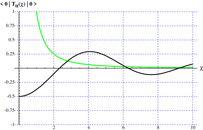
FIG. 1.: Spatial variation of the vacuum energy density for the discrete cutoff in two dimensions. Unlike the perfectly reflecting boundary vacuum energy, given by the lighter curve, the energy density for the discrete cutoff does not diverge as one approaches the interface. Here the energy density is expressed in units of ${2\xi\,{\omega_{c}}^{2}\over\pi}\left({{n_{0}-1}\over{n_{0}+1}}\right)$.

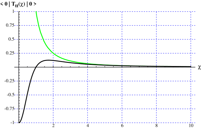
FIG. 2.: Spatial variation of the vacuum energy density for an exponentially decaying reflection coefficient in two dimensions. Near the dielectric mirror, the functional form of the vacuum energy density differs significantly from that of the perfectly reflecting mirror, given by the lighter curve. However, in the large $\chi$ limit, the dielectric mirror vacuum energy density reproduces the $\chi^{-2}$ behavior of the perfectly reflecting mirror. The energy density has been normalized to units of ${2\xi\,{\omega_{c}}^{2}\over\pi}$.

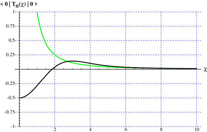
FIG. 3.: Spatial variation of the vacuum energy density for a Gaussian reflection coefficient in two dimensions. The energy density is expressed in units of ${2\xi\,{\omega_{c}}^{2}\over\pi}$. The vacuum energy density for a perfect reflector is given by the lighter curve.

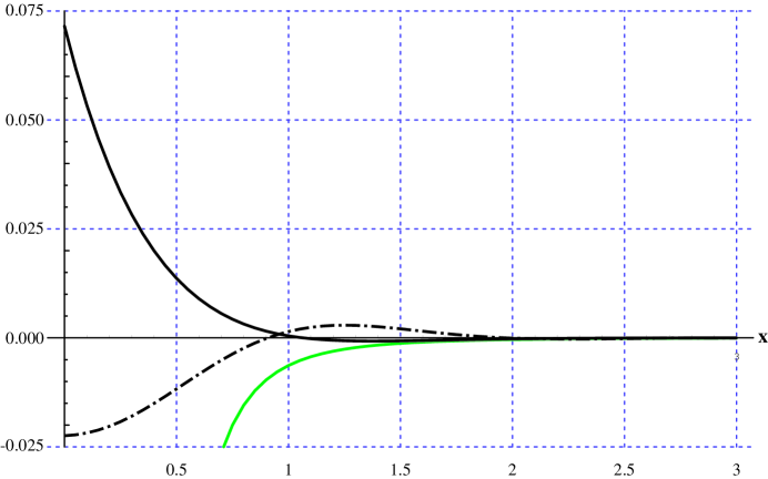
FIG. 4.: Numerical simulation of the $T_{tt}$ and $T_{ll}$ components of the vacuum stress-tensor, solid and dashed lines respectively, in the free space region for a planar frequency dependent dielectric to vacuum interface in four dimensions. The wave equation for the scalar field has minimal coupling and the model of the index of refraction is $n(\omega)=1+3\exp(-w^{2})$. The lighter line is the case of the perfect reflector.

REFERENCES

- [1] S. A. Fulling, Aspects of Quantum Field Theory in Curved Spacetime (Cambridge University Press, Cambridge, 1989).
- [2] N. D. Birrell and P. C. W. Davies, Quantum Fields in Curved Space, Cambridge Monographs on Mathematical Physics (Cambridge University Press, Cambridge, 1982).
- [3] L. H. Ford and N. F. Svaiter, Phys. Rev. D 58, (1998).
- [4] G. Barton and C. Eberlein, Ann. Phys. 227, 222 (1993).
- [5] A. D. Helfer, hep-th/0001004 (unpublished).
- [6] P. Candelas, Phys. Rev. D 21, 2185 (1980).
- [7] A. D. Helfer and A. S. I. D. Lang, J. Phys. A: Math. Gen. 32, 1937 (1998).
- [8] J. D. Jackson, Classical Electrodynamics, 2nd ed. (John Wiley & Sons, New York, 1962), see Section 7.5.
- [9] C. M. Bender and S. A. Orszag, Advanced Mathematical Methods for Scientists and Engineers, International Series in Pure and Applied Mathematics (McGraw-Hill, Inc., New York, 1978), see Section 6.5 on method of stationary phase.