Universal Aspects of Gravity Localized on Thick Branes

Abstract:

We study gravity in backgrounds that are smooth generalizations of the RandallSundrum model, with and without scalar fields. These generalizations include three-branes in higher dimensional spaces which are not necessarily Anti-de Sitter far from the branes, intersecting brane configurations and configurations involving negative tension branes. We show that under certain mild assumptions there is a universal equation for the gravitational fluctuations. We study both the graviton ground state and the continuum of Kaluza-Klein modes and we find that the four-dimensional gravitational mode is localized precisely when the effects of the continuum modes decouple at distances larger than the fundamental Planck scale. The decoupling is contingent only on the long-range behaviour of the metric from the brane and we find a universal form for the corrections to Newton’s Law. We also comment on the possible contribution of resonant modes. Given this, we find general classes of metrics which maintain localized four-dimensional gravity. We find that three-brane metrics in five dimensions can arise from a single scalar field source, and we rederive the BPS type conditions without any a priori assumptions regarding the form of the scalar potential. We also show that a single scalar field cannot produce conformally-flat locally intersecting brane configurations or a $p$-brane in greater than $(p+2)$-dimensions.

1 Introduction

The proposal of Randall and Sundrum (RS) [2, 3] to localize gravity in the vicinity of a brane with non-vanishing tension in anti-de Sitter (AdS) space has recently attracted enormous attention (see, for example [4, 5], for previous relevant work, [6, 7, 8, 9, 10, 11, 12, 13, 14, 15, 16, 17, 18, 19, 20, 21, 22, 23, 24, 25], for more recent generalizations, [26, 27, 28, 29, 30, 31], for work on smooth brane scenarios, [32, 33, 34, 35, 36, 37, 38], for embeddings in string theory and supergravity, [39, 40, 41, 42, 43, 44, 45, 46, 47, 48], for the general relativity aspects and finally [49, 50, 51, 52, 53], for cosmological and phenomenological aspects). RS found that in a setup with a single brane, a negative bulk cosmological constant and a single large extra dimension (with the cosmological constant and brane tension tuned such that the effective four-dimensional cosmological constant vanishes) the solution to Einstein’s equation results in a single graviton zero mode, which is a consequence of the unbroken four-dimensional Poincaré invariance, and a continuum of Kaluza-Klein (KK) modes. Normally the presence of these continuum modes would render a setup like this unrealistic due to the large deviation from Newton’s Law the low energy continuum modes tend to induce. However, RS found that due to the suppression of the wavefunctions of the continuum modes close to the brane, their contribution to the Newton potential is highly suppressed, and therefore a realistic model with uncompactified extra dimensions could be built. This model has been generalized in [6] to models with intersecting branes with more than one uncompactified extra dimension, and also to include brane junctions [7, 8].

The branes in the RS setup and its generalizations mentioned above are included as static point-like external sources in the extra dimensions, with no dynamics to produce them. As was done in [28, 29, 30, 34, 27], one can find solutions to Einstein’s equation coupled to a single scalar field, where the scalar creates a domain wall—a “thick brane”—while the metric away from the brane asymptotes to a slice of AdS₅. Such domain wall solutions are obtained if the scalar potential originates from a superpotential (although as recently discussed in [38] this does not necessarily imply that the theory is embeddable into a five-dimensional supergravity theory). In this case the solutions found in [28, 29, 27] originate from a BPS equation. These domain walls were first found in [26]. It has been shown in [28, 29, 27] that, just like for the case of the infinitely thin branes of RS, there is a single normalizable graviton bound-state with zero energy. A particularly nice example of this sort has been recently worked out in detail in [31]. Similar BPS equations for intersecting domain walls in more than one extra dimension were found in [9, 10]; however, no explicit solutions to these equations are known yet.

In this paper we study generic properties of localized gravity on thick branes. In the first part of the paper we consider thick branes in one extra dimension and then generalize to an arbitrary number of extra dimensions. Instead of starting with a coupled gravity-scalar system, as in [28, 29], we “smear” the RS solution and its generalizations in such a way that the non-dynamical source terms correspond to a smeared (thick) brane in the background of a slowly varying negative bulk cosmological constant. We examine the spectrum of graviton modes and find necessary and sufficient conditions for such backgrounds to localize gravity on the branes. Besides general arguments about the ground state (some of which appear in [28, 31]), we also examine the behavior of the continuum modes. For a generic study, we use the WKB approximation for the “volcano-type potential”, which hints that when the metric falls off slowly enough from the brane the soft KK modes are suppressed sufficiently inside the brane so that their corrections to the Newton’s Law are negligible. In a more restricted set of generalizations of the RS solution we calculate this suppression more rigorously, and find qualitative agreement with the WKB result. This leads to necessary conditions of the quantum mechanical potential, and hence the background metric, in order for the KK modes to decouple. We find that the potential at large distances must fall off no faster than in the asymptotically AdS case in order for the KK modes to make a small contribution to Newton’s Law. This requirement is equivalent to demanding normalizability of the ground state graviton wavefunction. We also comment on the possible contributions of “quasi-bound-states”—resonant modes in the continuum spectrum whose wavefunctions are not suppressed at the location of the brane—and study their significance in a toy model. We next show how to generalize our results to situations in more than five dimensions. These scenarios could describe, for example, three-branes in more than five dimensions or higher-dimensional intersecting branes with a four-dimensional intersection. In the latter case, the thick brane background could be given by an appropriate smearing of the intersecting brane solution of [6], and again we find conditions on the long-distance behavior of the background metric in order for there to be localized gravity on the brane intersection.

We also study the relevance of background fields that create the branes. We find that the stress-tensor source terms for a general smearing of the RS solution can be obtained from a single scalar field, and we rederive the same BPS-type equations for this scalar field as [28, 29, 27]. This provides a particularly simple derivation of the BPS equations without an a priori assumption about the form of the scalar potential, and also emphasizes that this is the most general solution with a single scalar field. In the case of branes in higher dimensions the situation is more complicated. Contrary to the case of one extra dimension, we find that it is impossible to generate the desired background metric or sources of the stress tensor with a single scalar field. Nevertheless, the properties of the graviton in such backgrounds are studied in the same way as for the case of one extra dimension.

2 Backgrounds with four-dimensional Poincaré invariance

In general, we are interested in $d$-dimensional backgrounds which have a four-dimensional Poincaré symmetry (the restriction to four dimensions is unnecessary, but is the case most relevant for phenomenology):

$$ds^{2}\equiv g_{\mu\nu}dx^{\mu}\,dx^{\nu}=e^{-A(z)}\eta_{ab}\,dx^{a}\,dx^{b}+g_{ij}(z)dz^{i}\,dz^{j}\ .$$ (1)

Here, $x^{\mu}=(x^{a},z^{i})$, where $x^{a}$, for $a=0,\ldots,3$, are the usual coordinates of four-dimensional Minkowski space and $z^{i}=x^{i+3}$, for $i=1,\ldots,n$, are the coordinates on the $n=(d-4)$-dimensional transverse space. We will assume that $A(0)=0$, so that the four-dimensional metric at the origin in the transverse space is canonically normalized. In this present work we will concentrate, for the most part, on a more restricted set of metrics which are conformally flat; that is of the form

$$ds^{2}=e^{-A(z)}\big{(}\eta_{ab}\,dx^{a}\,dx^{b}-dz^{i}\,dz^{i}\big{)}\ ,$$ (2)

with a suitable choice of coordinates. Notice that when $d=5$, an arbitrary metric of the form (1) is conformally flat, so in that case (2) is perfectly general.

We will be interested, amongst other things, in smooth versions of the RS metric in five dimensions discussed in [2]. The metric is usually written in the form

$$ds^{2}=e^{-A(r)}\eta_{ab}\,dx^{a}\,dx^{b}-dr^{2}$$ (3)

with $A(r)=2k|r|$, but can be written in conformally-flat form with $A(z)\equiv A(r(z))=2\log(k|z|+1)$. One simple way to introduce thick brane is by smoothing out RS ansatz. For example, one can make a substitution $|r|\rightarrow\mu^{-1}\log\cosh(\mu r)$, although for practical purposes it is more convenient to smooth in the $z$-basis:

$$|z|\rightarrow\frac{1}{\mu}\log\cosh(\mu z)\,.$$ (4)

Here $\mu$ is an independent parameter which determines the thickness of the brane. In the RS limit, $\mu\gg k$, we expect that any additional fields will be localized near $z=0$, which will be assumed in much of the following discussion (we will comment on subtleties associated with smearing of the matter fields over the thickness of the brane later). On the other hand, for simplicity it is convenient to study the behaviour of the gravitational modes in a different limit $\mu\sim k$, where $A(z)$ depends on only one scale $k$, and we will do so in most of our examples. In this case the equivalent smoothing in conformally-flat coordinates can be written as $A(r)=2\log\cosh(kr)$, or equivalently $A(z)=\log(k^{2}z^{2}+1)$, [31]. This metric approaches the AdS form asymptotically for $|z|\gg 1/k$. However, we will also consider metrics which are more general and not necessarily asymptotic to an AdS space.

We first point out that smoothing of the RS solution can be performed without the addition of matter fields. Consider the five-dimensional case where the domain wall is generated by an explicit position dependent term in the gravity action, much in the spirit of the original Randall-Sundrum scenario. (We will later study gravity in the background of branes created by scalar fields, and find that the supersymmetric potential introduced in [28, 29] appears naturally in the solution of the field equations.) In the absence of fields other than gravity, we study the action

$$S=-\int d^{5}x\,\left[\sqrt{g}\left(\kappa^{-2}R+\Lambda(r)\right)+\sqrt{g_{(4)}}\,V(r)\right]\ .$$ (5)

Here $g=|{\rm det}\,g_{\mu\nu}|$, $g_{(4)}=|{\rm det}\,g_{ab}|$ is the determinant of the induced metric on the domain wall and $\kappa^{2}=M_{*}^{-3}$, where $M_{*}$ is the fundamental Plank scale in five dimensions. The function $V(r)$ will approximate a delta function which generates the domain wall, and $\Lambda(r)$ is roughly constant away from the domain wall and corresponds to the bulk cosmological constant. This action gives rise to a stress tensor

$$T_{\mu\nu}=\tfrac{1}{2}\left(\Lambda(r)\,g_{\mu\nu}+V(r)\,g_{ab}\,\delta_{\mu}^{a}\,\delta_{\nu}^{b}\right)\ .$$ (6)

We note that any stress tensor which is four dimensional Lorentz covariant can be decomposed in this way, and therefore is derivable from an action of the form (5). We are interested in actions which admit solutions of the form (3). The “bulk cosmological constant” and “brane tension” are then determined to be

$$\Lambda(r)=-3\kappa^{-2}A^{\prime}(r)^{2}\ ,\qquad V(r)=3\kappa^{-2}A^{\prime\prime}(r)\ .$$ (7)

For $A(r)=2k|r|$, this reproduces the original Randall-Sundrum system [2]. By choice of a static background metric (3) the four-dimensional effective cosmological constant must vanish, and the fine tuning of cosmological constant and brane tension is replaced by (7). Indeed, one can integrate out the extra dimension and check that the action (5) vanishes for the background metric (3), which is equivalent to vanishing of the four-dimensional cosmological constant.

We should comment that because this analysis does not depend on what type of field creates the domain walls, we can study solutions in which the domain walls have negative tension. For example, we can study smooth versions of the RS solution to the hierarchy problem [3], in which the transverse direction is compactified on an orbifold $S^{1}/{\mathbb{Z}}_{2}$. Branes are stuck at the two fixed planes of the orbifold action, one of which has positive tension and the other negative tension. In the RS scenario the metric has the form (3) with $A(r)=2k|r|$, $-r_{c}<r<r_{c}$, where it is understood that $r$ is periodic over an interval $2r_{c}$. In order to make the periodicity explicit, we can study a multiple cover of the circle, with

$$A(r)=\sum_{n\in{\mathbb{Z}}}k\left[r_{c}+(-1)^{n}\left(2r-(2n+1)\,r_{c}\right)\right]\,\theta(r-nr_{c})\,\theta((n+1)r_{c}-r)\ ,$$ (8)

where $\theta(r)$ is the usual step function. The brane tension is related to $A^{\prime\prime}(r)$, which has delta function singularities with positive coefficient for $r=0$ mod $2r_{c}$ and negative coefficient for $r=r_{c}$ mod $2r_{c}$. As before the solution can be smoothed by an appropriate smearing of the $\theta$-functions; for example,

$$\theta(x)\rightarrow\tilde{\theta}(x)\equiv\tfrac{1}{2}(\tanh(\mu x)+1)\ ,$$ (9)

where $\mu$ is, as described previously, a parameter which characterizes the thickness of the brane. An alternative smoothing procedure which may be useful for numerical calculation is a truncation of the Fourier expansion of the sawtooth:

$$A(r)\approx\frac{r_{c}}{2}-\frac{4r_{c}}{\pi^{2}}\sum_{0\leq n<N}\frac{1}{(2n+1)^{2}}\cos(\pi(2n+1)r/r_{c})\ .$$ (10)

We will also consider backgrounds that can be interpreted as three-branes embedded in spaces of dimension $d>5$ and also backgrounds which can be interpreted as intersections of higher dimensional branes with a four-dimensional intersection. In the latter cases, the question for these kinds of backgrounds is whether four-dimensional gravity is localized on the intersection. For example, we will consider smooth versions of the multi-dimensional patched AdS space with metric [6]

$$ds^{2}=\frac{1}{(1+k\sum_{i=1}^{n}|z^{i}|)^{2}}\big{(}\eta_{ab}\,dx^{a}\,dx^{b}-dz^{i}dz^{i}\big{)}\ .$$ (11)

This metric represents $n=d-4$ intersecting $(d-1)$-branes, which mutually intersect in four dimensions.

3 Universal Aspects

3.1 Gravitational Fluctuations

In this section we derive a universal equation for the effective four-dimensional gravitational fluctuations in the conformally-flat backgrounds described in the last section. The more demanding case of the general background (1) will be discussed separately in Sec. 3.4. This means that we study fluctuations of the metric (2) of the form

$$ds^{2}=e^{-A(z)}\big{(}(\eta_{ab}+h_{ab}(x,z))\,dx^{a}\,dx^{b}-dz^{i}\,dz^{i}\big{)}\ .$$ (12)

It will be convenient to define $h_{\mu\nu}$ to be a fluctuation whose only non-zero components are $h_{ab}$. We will use the transverse traceless gauge for these fluctuations, i.e. $\partial_{\mu}\,h^{\mu\nu}=0$ and $h^{\mu}_{\mu}=0$. We should note that there may be additional fluctuations not of the form (12) in transverse traceless gauge, but we will not comment on such modes here.

Since the metric (2) is manifestly conformally flat, it is convenient to use the the general form of the Einstein tensor for metrics of the form $g_{\mu\nu}=e^{-A}\tilde{g}_{\mu\nu}$ (see for example [54]):

$$G_{\mu\nu}=\widetilde{G}_{\mu\nu}+\tfrac{d-2}{2}\Big{[}\tfrac{1}{2}\widetilde{\nabla}_{\mu}A\,\widetilde{\nabla}_{\nu}A+\widetilde{\nabla}_{\mu}\widetilde{\nabla}_{\nu}A-\tilde{g}_{\mu\nu}\big{(}\widetilde{\nabla}_{\rho}\widetilde{\nabla}^{\rho}A-\tfrac{d-3}{4}\,\widetilde{\nabla}_{\rho}A\,\widetilde{\nabla}^{\rho}A\big{)}\Big{]}\ ,$$ (13)

where indices are raised and lowered with $\tilde{g}_{\mu\nu}$ in this context. Using the form of the Einstein tensor for linear perturbations about flat spacetime [54],

$$\delta\widetilde{G}_{\mu\nu}=\partial^{\rho}\partial_{\left(\nu\right.}h_{\left.\mu\right)\rho}-\tfrac{1}{2}\partial^{\rho}\partial_{\rho}\,h_{\mu\nu}-\tfrac{1}{2}\partial_{\mu}\partial_{\nu}h^{\rho}_{\rho}-\tfrac{1}{2}\eta_{\mu\nu}\left(\partial^{\rho}\partial^{\kappa}\,h_{\rho\kappa}-\partial^{\rho}\partial_{\rho}\,h^{\kappa}_{\kappa}\right),$$ (14)

the linearized perturbation of the Einstein tensor (13) becomes,

$$\begin{split}\delta G_{\mu\nu}&=\partial^{\rho}\partial_{\left(\nu\right.}h_{\left.\mu\right)\rho}-\tfrac{1}{2}\underline{\partial^{\rho}\partial_{\rho}\,h_{\mu\nu}}-\tfrac{1}{2}\partial_{\mu}\partial_{\nu}\,h^{\rho}_{\rho}-\tfrac{1}{2}\eta_{\mu\nu}\left(\partial^{\rho}\partial^{\kappa}\,h_{\rho\kappa}-\partial^{\rho}\partial_{\rho}\,h^{\kappa}_{\kappa}\right)\\ &-\tfrac{d-2}{2}\big{[}\tfrac{1}{2}\eta^{\rho\kappa}(\partial_{\mu}\,h_{\nu\rho}+\partial_{\nu}\,h_{\mu\rho}-\underline{\partial_{\rho}\,h_{\mu\nu}})\,\partial_{\kappa}\,A\\ &+\underline{h_{\mu\nu}\partial_{\rho}\partial^{\rho}A}+\eta_{\mu\nu}\left(-\partial_{\rho}\,h^{\rho\kappa}\,\partial_{\kappa}A+\tfrac{1}{2}\partial_{\rho}\,h^{\kappa}_{\kappa}\,\,\partial^{\rho}A-h^{\rho\kappa}\,\partial_{\rho}\partial_{\kappa}A\right)\\ &-\tfrac{d-3}{4}\big{(}\underline{h_{\mu\nu}\,\partial_{\rho}A\,\partial^{\rho}A}-\eta_{\mu\nu}\,h^{\rho\kappa}\partial_{\rho}A\,\partial_{\kappa}A\big{)}\big{]}\ .\end{split}$$ (15)

Only the terms which are underlined are actually non-zero. The other terms either vanish due to the gauge conditions or they vanish because $h_{\mu\nu}$ only has non-zero components $h_{ab}$ and, moreover, $A$ is a function of the $\{z^{i}\}$ only.

The next question concerns the variation of the stress tensor. For any action of the form (5)

$$\delta T_{\mu\nu}=T_{\mu}^{\kappa}\,h_{\kappa\nu}\ ,$$ (16)

which is automatically symmetric. Later we will show that this transformation property remains valid when the background is generated by scalar fields. From (16), and the unperturbed Einstein equation, we derive

$$\delta T_{\mu\nu}=\tfrac{d-2}{2}\kappa^{-2}(\tfrac{1}{2}\partial_{\mu}A\,\partial^{\kappa}A+\partial_{\mu}\partial^{\kappa}A)\,h_{\kappa\nu}+\tfrac{d-2}{2}\kappa^{-2}(-\underline{\partial_{\rho}\partial^{\rho}A}+\tfrac{d-3}{4}\,\underline{\partial_{\rho}A\,\partial^{\rho}A})h_{\mu\nu}\ .$$ (17)

Again only the underlined terms survive due to either the gauge conditions or the particular choice of background. Both the surviving terms of $\delta T_{\mu\nu}$ cancel with two terms of $\delta G_{\mu\nu}$ in the graviton equation of motion $\delta G_{\mu\nu}-\kappa^{2}\delta T_{\mu\nu}=0$, leaving

$$-\tfrac{1}{2}\partial^{\rho}\partial_{\rho}\,h_{\mu\nu}+\tfrac{d-2}{4}\,\partial^{\rho}A\,\,\partial_{\rho}\,h_{\mu\nu}=0\ .$$ (18)

If we redefine the metric perturbation so that its kinetic term has the canonical normalization, i.e. ${h}_{\mu\nu}=e^{(d-2)A/4}\,\tilde{h}_{\mu\nu}$, then the term linear in derivatives is removed:

$$-\tfrac{1}{2}\partial^{\rho}\partial_{\rho}\,\tilde{h}_{\mu\nu}+\Big{[}\tfrac{(d-2)^{2}}{32}\partial^{\rho}A\partial_{\rho}A-\tfrac{d-2}{8}\partial^{\rho}\partial_{\rho}A\Big{]}\tilde{h}_{\mu\nu}=0\ .$$ (19)

We should emphasize that indices are raised and lowered here using the flat metric $\eta_{\mu\nu}$. In addition, only the $h_{ab}$ components of the fluctuation $h_{\mu\nu}$ are non-vanishing.

Now we use the fact that $\partial^{\rho}\partial_{\rho}=-\square_{x}-\nabla_{z}^{2}$, where $\square_{x}=-\eta^{ab}\partial_{a}\partial_{b}$ and $\nabla_{z}^{2}=\partial_{i}^{2}$, and look for solutions of the form $\tilde{h}_{ab}(x,z)=\check{h}_{ab}(x)\psi(z)$ with $\square_{x}\check{h}_{ab}(x)=m^{2}\check{h}_{ab}(x)$, where $m$ is the four-dimensional Kaluza-Klein mass of the fluctuation. Then since $A=A(z)$ only, we have

$$-\nabla_{z}^{2}\psi(z)+\Big{[}\tfrac{(d-2)^{2}}{16}\nabla_{z}A\cdot\nabla_{z}A-\tfrac{d-2}{4}\nabla_{z}^{2}A\Big{]}\psi(z)=m^{2}\psi(z)\ .$$ (20)

This has the form of a Schrödinger equation for the “wavefunction” $\psi(z)$, “energy” $m^{2}$ and potential

$$V(z)=\tfrac{(d-2)^{2}}{16}\nabla_{z}A(z)\cdot\nabla_{z}A(z)-\tfrac{d-2}{4}\nabla_{z}^{2}A(z)\ .$$ (21)

The fact that when expressed in terms of the variable $\tilde{h}_{\mu\nu}$, the graviton equations-of-motion (19) have no single derivative terms is equivalent to the fact that the action for these fluctuations has the form of a canonical kinetic term:

$$S\thicksim\int d^{d}x\,\partial_{\rho}\tilde{h}_{\mu\nu}\partial^{\rho}\tilde{h}^{\mu\nu}\ ,$$ (22)

where indices are contracted with the flat metric $\eta_{\mu\nu}$. This can be seen by expanding the scalar curvature about the background (2) and keeping track of powers of the conformal factor in the metric. (If we had chosen coordinates in which the metric is not explicitly in the conformally-flat form, then the kinetic terms in the $x$ and $z$ directions would have had different conformal factors multiplying them.) The redefinition of the metric $h_{\mu\nu}=e^{(d-2)A(z)/4}\tilde{h}_{\mu\nu}$ then absorbs the conformal factor multiplying the kinetic terms and puts the action in the canonical form (22). In particular, for solutions in the form $\check{h}_{ab}(x)\psi(z)$, (22) includes the term

$$\int d^{n}z\,\psi(z)^{2}\,\cdot\,\int d^{4}x\,\partial_{c}\,\check{h}_{ab}(x)\,\partial^{c}\,\check{h}^{ab}(x)\ ,$$ (23)

from which we deduce that the appropriate inner-product for the “wavefunctions” $\psi(z)$ is the conventional quantum mechanical one. (Notice that this differs from the inner-product employed in [28].)

In order to calculate the strength of the four-dimensional gravitational coupling, it is convenient to decompose the action into a four dimensional part and higher dimensional parts, before rescaling the graviton. As in [2, 6], including the fundamental ($d$-dimensional) Planck scale $M_{*}$, which is related to the coupling $\kappa$ via

$$\kappa^{2}=M^{2-d}_{*}\ ,$$ (24)

the action takes the form,

$$S\thicksim M^{d-2}_{*}\int d^{n}z\,e^{-(d-2)A/2}\,\cdot\,\int d^{4}x\,\sqrt{\hat{g}_{(4)}}\,R^{(4)}+\cdots,$$ (25)

where $\hat{g}_{(4)}$ is the determinant of the four-dimensional metric for matter perturbations about flat spacetime, and $R^{(4)}$ is the four-dimensional curvature scalar created by those matter perturbations. This allows us to identify the four-dimensional Planck scale $M_{4}$ via,

$$M_{4}^{2}=M^{d-2}_{*}\,\int d^{n}z\,e^{-(d-2)A(z)/2}\ ,$$ (26)

and determines the four dimensional gravitational coupling $G_{N}\sim M_{4}^{-2}$.

3.2 The four-dimensional graviton

The question of whether there is localized (four-dimensional) gravity supported in the vicinity of the brane now becomes contingent on properties of the quantum mechanical system described by the Schrödinger equation (20). In particular, in order to have an effective four-dimensional theory of gravity we require that (20) admits a normalizable zero-energy ground state. To find this zero-energy state, we notice, generalizing the observation of [28, 35] to higher dimensions, that the Schrödinger equation (20) can be rewritten as a supersymmetric quantum mechanics problem of the form,

$$Q^{\dagger}\cdot Q\,\psi(z)=m^{2}\psi(z)\ ,$$ (27)

where the $n$-vector of supersymmetry charge is

$$Q=\nabla_{z}+\tfrac{d-2}{4}\nabla_{z}A\ ,\qquad Q^{\dagger}=-\nabla_{z}+\tfrac{d-2}{4}\nabla_{z}A\ .$$ (28)

Hence, the zero-energy wavefunction, annihilated by $Q$, is

$$\hat{\psi}_{0}(z)=\exp\big{[}-\tfrac{d-2}{4}A(z)\big{]}\ .$$ (29)

Notice that such a wavefunction always exists since (18) always admits the solution where $h_{ab}=h_{ab}(x)$, only, and $\square_{x}h_{ab}(x)=0$. Furthermore, since the “Hamiltonian” $Q^{\dagger}\cdot Q$ is a positive definite Hermitian operator, there are no normalizable negative energy graviton modes, as required for stability of the gravitational background.

The condition for having localized four-dimensional gravity is that $\hat{\psi}_{0}(z)$ is normalizable; in other words

$$\int d^{n}z\,\exp\big{[}-\tfrac{d-2}{2}A(z)\big{]}<\infty\ .$$ (30)

Notice that normalizability of the ground state wavefunction is equivalent to the condition that the four-dimensional gravitational coupling (via (26)) be non-vanishing; indeed

$$G_{N}\sim\frac{M^{2-d}_{*}\hat{\psi}_{0}(0)^{2}}{\langle\hat{\psi}_{0}|\hat{\psi}_{0}\rangle}\ .$$ (31)

This requires that $A(z)\to\infty$ sufficiently fast as $|z|\to\infty$. Normalizability is intimately connected with the asymptotic behaviour of the potential of the Schrödinger equation (20). If $V(z)>0$ as $|z|\to\infty$, then $\hat{\psi}_{0}(z)$ is always normalizable. On the contrary, if $V(z)<0$ as $|z|\to\infty$, then $\hat{\psi}_{0}(z)$ is not normalizable and therefore is of no interest to us since it cannot describe localized four-dimensional gravity. The situation where $V(z)=0$ as $|z|\to\infty$, is, perhaps, the most interesting and we will focus on that case in most of the remainder of this paper.

At this point, we make the obvious remark that in any scenario where the transverse space is asymptotically flat Euclidean space ($A(z)\to$ constant, as $|z|\to\infty$) $\hat{\psi}_{0}(z)$ is non-normalizable and gravity cannot be localized.

3.3 Corrections to Newton’s Law

In order to have localized four-dimensional gravity, we also require that the other solutions of the Schrödinger equation (20), the KK modes, do not lead to unacceptably large corrections to Newton’s Law in the four-dimensional theory.

In any realistic brane scenario, the matter fields in the four-dimensional theory on the brane would be smeared over the width of the brane in the transverse space. Rather than deal with this complication, we will, for simplicity, consider the gravitational potential between two point-like sources of mass $M_{1}$ and $M_{2}$ located at the origin, $z^{i}=0$, in the transverse space [2, 6, 35]. This assumption is justified in cases when the thickness of the brane is small compared with the bulk curvature. We expect that our conclusions will be at least qualitatively correct in a general case and present some supporting arguments in Sec. 6. In order to evaluate the correction to Newton’s Law, we note that a discrete eigenfunction (these are not present in the RS case) of the Schrödinger equation $\psi_{m}(z)$ of energy $m^{2}$ acts in four-dimensions like a field of mass $m$ and consequently contributes a Yukawa-like correction to the four-dimensional gravitational potential between two masses $M_{1}$ and $M_{2}$:

$$U(r)\thicksim G_{N}\frac{M_{1}M_{2}}{r}+M^{2-d}_{*}\frac{M_{1}M_{2}e^{-mr}}{r}\psi_{m}(0)^{2}$$ (32)

where the wavefunction $\psi_{m}(z)$ is normalized $\int d^{n}z\,\psi_{m}(z)^{2}=1$. As long as $m$ is large enough, this will be a small correction. The fact that $\psi_{m}(0)$ appears in (32) is due to our simplifying assumption that the sources are point-like and located at $z^{i}=0$. A more complete analysis would involve the effects of the overlap of the gravitational modes with the matter modes, and would correct the factors of $\psi_{m}(0)$. We will not have more to say about such corrections here.

The correction from any continuum states $\psi_{m}(z)$ is obtained by integrating over these states with the relevant density-of-states measure. For states which form a continuum in $n$-dimensions starting at $m_{0}$ the correction to Newton’s Law is

$$U(r)\thicksim G_{N}\frac{M_{1}M_{2}}{r}+M^{2-d}_{*}\int_{m_{0}}^{\infty}dm\,m^{n-1}\,\frac{M_{1}M_{2}e^{-mr}}{r}\psi_{m}(0)^{2}\ ,$$ (33)

where the wavefunctions $\psi_{m}(z)$ of the continuum are normalized as plane waves, i.e. to unity over a period at $|z|\to\infty$. The factor of $m^{n-1}$ is just the $n$-dimensional plane wave continuum density of states (up to a constant angular factor). Notice that in flat $d$-dimensional space there would be no normalizable zero-energy wavefunction $\hat{\psi}_{0}(z)$ and the continuum would extend down to $m=0$ and be unsuppressed: $\psi_{m}(0)=1$. In such a case $U(r)\sim M_{1}M_{2}M^{2-d}_{*}r^{-n-1}=M_{1}M_{2}M^{2-d}_{*}r^{3-d}$, as expected for the gravitational potential in $d$-dimensions.

In the case of intersecting branes, there are continuum modes which are localized in a subset of the transverse dimensions. In other words, the wavefunctions behave as plane waves only in $p<n$ of the transverse dimensions. In this case the corrections from this part of the continuum spectrum are of the form (33) with $n$ replaced by $p$.

For the case when $V(z)>0$ as $|z|\to\infty$, the excited states are clearly separated by a gap from the ground-state. Hence corrections to Newton’s Law are exponentially suppressed as in (32). As we have already mentioned, the most interesting case is where the potential goes to zero at infinity. In this case there is a continuum of scattering states $\psi_{m}(z)$ with eigenvalues $m^{2}\geq 0$ and so the behaviour of the soft modes at $z^{i}=0$ is crucial for determining whether the corrections are small.

3.4 Extension to non-conformally-flat backgrounds

In this section, we briefly indicate how the preceding analysis of gravitational fluctuations extends to cases where the background is of the general non-conformally flat form (1). In order to derive an equation for metric fluctuations

$$ds^{2}=e^{-A(z)}(\eta_{ab}+h_{ab}(x,z))\,dx^{a}\,dx^{b}-g_{ij}(z)dz^{i}\,dz^{j}\ ,$$ (34)

we follow essentially the same steps as for the conformally-flat case detailed in Sec. 3.1. First of all, it is convenient to define the metric $\tilde{g}_{\mu\nu}(z)=e^{A(z)}g_{\mu\nu}(z)$ and apply the relation (13) in order to find the variation of the Einstein tensor $G_{\mu\nu}$. Rather than writing down all of the terms, as we did in Sec. 3.1, we will make immediate use of the following four facts: (i) $\partial_{\mu}h^{\mu\nu}=0$; (ii) $h^{\mu}_{\mu}=0$; (iii) $g_{\mu\nu}$ only depends on $z$; and (iv) the only non-vanishing components of the variation $h_{\mu\nu}$ are $h_{ab}$. By brute force one can show that the variation of the Einstein tensor $\widetilde{G}_{\mu\nu}$ is

$$\begin{split}\delta\widetilde{G}_{\mu\nu}=-\tfrac{1}{2}\tilde{\nabla}^{\rho}\tilde{\nabla}_{\rho}h_{\mu\nu}=-\tfrac{1}{2}\partial^{c}\partial_{c}h_{\mu\nu}-\tfrac{1}{2}\tilde{g}^{-1/2}\partial_{i}(\sqrt{\tilde{g}}\tilde{g}^{ij}\partial_{j}h_{\mu\nu})\ ,\end{split}$$ (35)

where, until further notice, indices are raised and lowered with $\tilde{g}_{\mu\nu}$. Using (13), we can then write down the variation of the original Einstein tensor:

$$\begin{split}\delta{G}_{\mu\nu}&=-\tfrac{1}{2}\partial^{c}\partial_{c}h_{\mu\nu}-\tfrac{1}{2}\tilde{g}^{-1/2}\partial_{i}(\sqrt{\tilde{g}}\tilde{g}^{ij}\partial_{j}h_{\mu\nu})+\tfrac{d-2}{4}\partial_{i}A\partial^{i}h_{\mu\nu}\\ &\qquad\qquad\qquad\qquad+\tfrac{d-2}{2}\big{(}-\tilde{g}^{-1/2}\partial_{i}(\sqrt{\tilde{g}}\tilde{g}^{ij}\partial_{j}A)+\tfrac{d-3}{4}\partial_{i}A\partial^{i}A\big{)}h_{\mu\nu}\ .\end{split}$$ (36)

Assuming that the variation of the stress-tensor is given by (16), we have

$$\delta T_{\mu\nu}=\tfrac{d-2}{2}\kappa^{-2}\big{(}-\tilde{g}^{-1/2}\partial_{i}(\sqrt{\tilde{g}}\tilde{g}^{ij}\partial_{j}A)+\tfrac{d-3}{4}\kappa^{-2}\partial_{i}A\partial^{i}A\big{)}h_{\mu\nu}\ .$$ (37)

Hence, Einstein’s equation gives

$$-\tfrac{1}{2}\partial^{c}\partial_{c}h_{\mu\nu}-\tfrac{1}{2}\tilde{g}^{-1/2}\partial_{i}(\sqrt{\tilde{g}}\tilde{g}^{ij}\partial_{j}h_{\mu\nu})+\tfrac{d-2}{4}\partial_{i}A\partial^{i}h_{\mu\nu}=0\ ,$$ (38)

which can be rewritten in terms of the original metric as

$$\frac{1}{\sqrt{g}}\partial_{\rho}\big{(}\sqrt{g}g^{\rho\kappa}\,\partial_{\kappa}h_{\mu\nu}\big{)}=0\ ,$$ (39)

where now indices are raised and lowered with $g_{\mu\nu}$. In other words, the general equation for the fluctuations is simply the covariant scalar wave-equation. This has been noted in the case of one transverse dimension in [35] which also discusses its significance within the AdS/CFT correspondence. For a conformally-flat background (39) reduces to (18).

For a fluctuation of the form $h_{ab}(x,z)=\varphi(z)\check{h}_{ab}(x)$, with $\square_{x}\check{h}_{ab}(x)=m^{2}\check{h}_{ab}(x)$, we have

$$-\frac{1}{\sqrt{g}}\partial_{i}\big{(}\sqrt{g}g^{ij}\,\partial_{j}\varphi(z)\big{)}=m^{2}g^{00}\varphi(z)\ .$$ (40)

This describes the $z$-dependence of a mode with four-dimensional Kaluza-Klein mass $m$. Notice that when $m=0$ (40) always admits the solution $\varphi(z)=$ constant; this will lead to the analogue of the zero-energy solution $\hat{\psi}_{0}(z)$ in the conformally-flat case. The fluctuation equation (39) is derivable from the action

$$S\thicksim\int d^{d}x\,\sqrt{g}\partial_{\rho}h_{\mu\nu}\partial^{\rho}h^{\mu\nu}=\int d^{n}z\,g^{00}(z)\sqrt{g(z)}\varphi(z)^{2}\cdot\int d^{4}x\,\partial_{c}\check{h}_{ab}(x)\partial^{c}\check{h}^{ab}(x)+\cdots\ .$$ (41)

From the $z$-integral above, inserting $\varphi(z)=$ constant, we deduce the generalized expression for the zero-energy “wavefunction” $\hat{\psi}_{0}(z)$:

$$\hat{\psi}_{0}(z)=\big{[}g^{00}(z)\sqrt{g(z)}\,\big{]}^{1/2}\ ,$$ (42)

which reduces to (29) in the conformally-flat case. The normalizability condition is consequently

$$\int d^{n}z\,g^{00}(z)\sqrt{g(z)}<\infty\ .$$ (43)

The “wavefunction” is consequently

$$\psi(z)\equiv\varphi(z)\big{[}g^{00}(z)\sqrt{g(z)}\,\big{]}^{1/2}\ ,$$ (44)

which satisfies a generalization of the Schrödinger equation (20):

$$-\frac{1}{[g^{00}\sqrt{g}\,]^{1/2}}\partial_{i}\Big{(}\sqrt{g}g^{ij}\,\partial_{j}\frac{\psi(z)}{[g^{00}\sqrt{g}\,]^{1/2}}\Big{)}=m^{2}\psi(z)\ .$$ (45)

4 Gravity Localized on Thick Three-Branes

In this section we consider in some detail the case when the 3-brane is embedded in a space with dimension $d\geq 5$. We will, as per Sec. (2), restrict ourselves mainly to a conformally-flat background which is, in addition, radially symmetric in the space transverse to the brane. In other words we shall consider metrics of the form

$$ds^{2}=e^{-A(\varrho)}\big{(}\eta_{ab}\,dx^{a}\,dx^{b}-d\varrho^{2}-\varrho^{2}d\Omega^{2}\big{)}\ ,$$ (46)

where $\varrho$ is the radial coordinate in the transverse directions and $\Omega$ are the angular coordinates on $S^{d-5}$. The function $A(\varrho)$, as indicated, only depends on the radial variable. We will briefly consider the more general radially symmetric background which is not necessarily conformally flat at the end of Sec. 4.4.

4.1 Localization and decoupling in $d=5$

We begin by discussing the case in $d=5$, corresponding to the RS scenario, when the transverse space is one-dimensional. In this case, the metric (46) is

$$ds^{2}=e^{-A(z)}\big{(}\eta_{ab}\,dx^{a}\,dx^{b}-dz^{2}\big{)}\ .$$ (47)

The Schrödinger equation (20) is:

$$-\frac{d^{2}\psi(z)}{dz^{2}}+\big{[}\tfrac{9}{16}A^{\prime}(z)^{2}-\tfrac{3}{4}A^{\prime\prime}(z)\big{]}\psi(z)=m^{2}\psi(z)\ .$$ (48)

The zero-energy state (29) is [29, 31]

$$\hat{\psi}_{0}(z)=\exp\big{[}-\tfrac{3}{4}A(z)\big{]}\ .$$ (49)

For this to be normalizable, $\exp[-\tfrac{3}{2}A(z)]$ must fall off faster than $1/z$. As we explained in Sec. 3.2, the question of whether $\hat{\psi}_{0}(z)$ is normalizable is intimately connected with the asymptotic behaviour of the potential $V(z)$. If $V(z)>0$ as $|z|\to\infty$, then $\hat{\psi}_{0}(z)$ is always normalizable. On the contrary, if $V(z)<0$ as $|z|\to\infty$, then $\hat{\psi}_{0}(z)$ is not normalizable and therefore is no interest to us since it cannot describe localized four-dimensional gravity.

The fact that there are no bound-states with negative energy follows from the factorization (27):

$$\Big{[}-\frac{d}{dz}+\frac{3}{4}A^{\prime}(z)\Big{]}\Big{[}\frac{d}{dz}+\frac{3}{4}A^{\prime}(z)\Big{]}\psi(z)=m^{2}\psi(z)\ ,$$ (50)

which has the form of supersymmetric quantum mechanics $Q^{\dagger}Q\psi(z)=m^{2}\psi(z)$, with $Q\equiv d/dz+\tfrac{3}{4}A^{\prime}(z)$. Hence the zero-energy state (49), which satisfies the supersymmetric condition $Q\hat{\psi}_{0}(z)=0$, is the ground state, the bound-state of lowest energy.

The borderline case, $V(z)\to 0$ as $|z|\to\infty$, is the most interesting case, and includes smoothed versions of the AdS scenario of [2]. For example, when the wavefunction (29) has a power-law fall-off $\psi(z)\sim|z|^{-\alpha}$, then normalizability requires $\alpha>\tfrac{1}{2}$. In this case the potential $V(z)$ falls off as $\alpha(\alpha+1)/z^{2}$. Conversely, if we assume that the potential falls off as $|z|^{-2\beta}$ the wavefunction $\hat{\psi}_{0}(z)$ falls off as $e^{-c/|z|^{\beta-1}}$. Consequently, if $\beta<1$, then the wavefunction is not normalizable. It is interesting to note that the borderline case, where the potential falls off just slowly enough to give rise to a normalizable bound-state, i.e. $V(z)\sim|z|^{-2}$, includes the AdS scenario. Figure 1 shows the potential $V(z)$ for a particular smoothing of the AdS case with $A(z)=\log(k^{2}z^{2}+1)$, discussed in Sec. 4.2.

Figure 1: The Schrödinger potential (21) for the case $A(z)=\log(k^{2}z^{2}+1)$.

We now have to consider the question of whether or not the other modes in our problem decouple. The relevant effects of these modes on Newton’s Law were established in Sec. 3.3. For the case when $V(z)>0$, for $|z|\to\infty$, the excited states are clearly separated by a gap from the ground-state. Hence corrections to Newton’s Law will be exponentially suppressed, as in (32). The most interesting case is where the potential goes to zero at infinity. In this case there is a continuum of scattering states $\psi_{m}(z)$ with eigenvalues $m^{2}\geq 0$. Since the bottom of the continuum is at $m=0$ it is clear that decoupling is a delicate issue. From (33), given that gravity is localized so that $\hat{\psi}_{0}(z)$ is normalizable, decoupling would require that $\int_{0}^{\infty}dm\,e^{-mr}|\psi_{m}(0)|^{2}$ has no singularity at the bottom limit of integration.

Before we attempt some rigorous analysis, let us consider the problem with some rather crude apparatus. If the continuum modes are to decouple we want the probability for continuum modes to tunnel into the central region of the potential to be vanishingly small for $m\to 0$. In order to get a feeling for what might be required, it is instructive to consider the WKB approximation for this tunneling probability. Consider a continuum mode with energy $m^{2}$ incident upon the potential from the right. The transition probability is, in the WKB approximation,

$$T(m)\thicksim\exp\Big{[}-2\int_{z_{0}(m)}^{z_{1}(m)}dz\,\sqrt{V(z)-m^{2}}\Big{]}\ ,$$ (51)

where $0<z_{0}(m)<z_{1}(m)$ are the two points in the rightmost barrier region where $V(z)=m^{2}$. In order for the soft continuum states to decouple we would need $T(0)=0$. Since $z_{1}(0)=\infty$, this can be achieved if the integral (51) has a divergence for large $z$; in other words, if $V(z)$ falls off at least as slowly as $1/z^{2}$. This matches precisely the condition on the normalizability of the state $\hat{\psi}_{0}(z)$. This suggests that there is a natural decoupling of the continuum states precisely when the ground state $\hat{\psi}_{0}(z)$ is normalizable.

So the hypothesis that we want to establish is that the continuum modes decouple (that is lead to small corrections to Newton’s Law) precisely when $\hat{\psi}_{0}(z)$ is normalizable. To this end, consider a potential of the form

$$V(z)\sim\frac{\alpha(\alpha+1)}{z^{2}}\ ,$$ (52)

for large $|z|$. We shall find that the crossover from localization to de-localization occurs for some critical value of $\alpha$. We shall not assume any particular form for the potential $V(z)$ except, for simplicity, that it only depends on a single dimensionful scale $k$, so that, for instance, the central region extends over a scale $1/k$; in other words (52) is valid for $|z|\gg 1/k$.

As we have discussed above, what we need to calculate in order to investigate the decoupling of the continuum modes is the limiting behaviour of $\psi_{m}(0)$ at small $m$. Let us consider four different regions in $z$ (we will always be considering modes with energies $m\ll k$): (1) $z\ll 1/k$, (2) $1/k\ll z\ll 1/m$, (3) $1/k\ll z\sim 1/m$ and (4) $1/m\ll z$. In regions (2),(3) and (4), we must solve the Schrödinger equation with the tail of the potential (52):

$$-\frac{d^{2}\psi_{m}(z)}{dz^{2}}+\frac{\alpha(\alpha+1)}{z^{2}}\psi_{m}(z)=m^{2}\psi_{m}(z)\ .$$ (53)

The solution is given by a linear combination of Bessel functions

$$\psi_{m}(z)=a_{m}z^{1/2}Y_{\alpha+1/2}(mz)+b_{m}z^{1/2}J_{\alpha+1/2}(mz)\ .$$ (54)

In region (4), where $mz\gg 1$, the Bessel functions become plane waves:

$$\psi_{m}(z)=a_{m}\sqrt{\frac{2}{\pi m}}\sin(mz-\tfrac{\pi}{2}\alpha-\tfrac{\pi}{2})+b_{m}\sqrt{\frac{2}{\pi m}}\cos(mz-\tfrac{\pi}{2}\alpha-\tfrac{\pi}{2})\ .$$ (55)

In region (2), where $mz\ll 1$ (but $kz\gg 1$), the Bessel functions can be expanded in $mz$ giving

$$\begin{split}\psi_{m}(z)=-\frac{a_{m}z^{1/2}\Gamma(\alpha+1/2)}{\pi}\left(\frac{2}{mz}\right)^{\alpha+1/2}&\Big{[}1+\frac{1}{\alpha-1/2}\left(\frac{mz}{2}\right)^{2}+\cdots\Big{]}\\ &+\frac{b_{m}z^{1/2}}{\Gamma(\alpha+3/2)}\left(\frac{mz}{2}\right)^{\alpha+1/2}\Big{[}1+\cdots\Big{]}\ .\end{split}$$ (56)

In other words we can match the wavefunction in regions (2) and (4) by using the asymptotic behavior of the Bessel functions, and the exact form of the Bessel function then determines the behavior in the intermediate region, (3).

Now we show how to match regions (1) and (2). In these regions $mz\ll 1$ and it is meaningful to solve the Schödinger equation as a series in $m^{2}$. The first two terms are

$$\psi_{m}(z)=\hat{\psi}_{0}(z)+m^{2}\phi(z)+\cdots\ ,$$ (57)

where $\hat{\psi}_{0}(z)$ is the suitably normalized zero energy solution (29). The first correction $\phi(z)$ satisfies the inhomogeneous equation

$$\Big{[}-\frac{d^{2}}{dz^{2}}+V(z)\Big{]}\phi(z)=\hat{\psi}_{0}(z)\ .$$ (58)

Now we can match (57) with $z\gg 1/k$, with the series in region (2) (56). In this region $\hat{\psi}_{0}(z)\sim z^{-\alpha}$, which matches the first term in (56) if $a_{m}\sim m^{\alpha+1/2}$. The second and third terms in (56) then match the next term in the expansion (57) as long as $b_{m}\sim m^{-\alpha+3/2}$. Using this matching procedure, we have determined the $m$-dependence of $a_{m}$ and $b_{m}$. Since $m$ is small, the dominant term in region (4) comes from the second term in (55) where the coefficient of the cosine goes like $b_{m}m^{-1/2}\sim m^{-\alpha+1}$. Hence to normalize the wavefunction $\psi_{m}(z)$ as a plane wave, we must multiple it by an overall factor of $m^{\alpha-1}$. The value of the wavefunction at $z=0$ is then extracted from (57). To leading order in $m$,

$$\psi_{m}(0)\thicksim\left(\frac{m}{k}\right)^{\alpha-1}\ ,$$ (59)

where the factor of $k$ is dictated by dimensional analysis. Notice that in the AdS scenario of [2], $\alpha=\tfrac{3}{2}$, in which case we find $\psi_{m}(0)^{2}\sim m/k$, in agreement with the exactly solved delta-function potential of [2].

Equation (59) establishes the asymptotic behaviour of the continuum modes at $z\ll 1/k$, where $k$ is characteristic decay width of the potential $V(z)$. If the matter is smeared over the distances $1/k$ one needs to obtain more information about the wave-functions of the excited modes to study the corrections to the Newton’s Law. It is important to note, however, that we obtained (59) without specifying details of the potential near $z=0$. Thus, we can easily introduce a potential such that matter is localized near $z=0$, yet the arguments leading to (59) remain valid.

From (59), we find that the integral over the continuum modes in (33) is only non-singular at the bottom limit of integration if $\alpha>\tfrac{1}{2}$. In this case the corrections are

$$U(r)\thicksim G_{N}\frac{M_{1}M_{2}}{r}+\frac{C}{M^{3}_{*}k^{2\alpha-2}}\frac{M_{1}M_{2}}{r^{2\alpha}}=G_{N}\frac{M_{1}M_{2}}{r}\Big{(}1+\frac{C^{\prime}}{(kr)^{2\alpha-1}}\Big{)}\ ,$$ (60)

where $C$ and $C^{\prime}$ are dimensionless numbers. We are assuming that the metric only depends on one dimensionful parameter $k$, so that $G_{N}\sim kM^{-3}_{*}$. Notice that when the potential falls off as (52) there are power-law corrections to Newton’s Law with a universal exponent $\alpha$ determined simply by the long-range fall-off of the potential. We emphasize that the AdS case of [2] corresponds to taking $\alpha=\tfrac{3}{2}$, which agrees with the exact calculation of the correction presented in [2].

Now we see that it is precisely when $\hat{\psi}_{0}(z)$ is normalizable, i.e. when $\alpha>\tfrac{1}{2}$, that the continuum states give a correction to Newton’s Law which is suppressed relative to the leading term.

4.2 Examples

At this point it is probably worthwhile to consider some examples. To begin with, consider the class of conformally-flat five dimensional backgrounds for which

$$A(z)=\tfrac{2\alpha}{3}\log(k^{2}z^{2}+1)\ ,$$ (61)

for some constants $\alpha$. The case when $\alpha=\tfrac{3}{2}$ is particularly interesting because in this case we can easily transform back to the $r$ coordinate in which case $A(r)=2\log\,\cosh(kr)$. So when $\alpha=\tfrac{3}{2}$ the space given by (61) is asymptotically AdS and therefore represents a smoothing of the AdS example of [2], recently discussed in [31].

For general $\alpha$, the potential in the Schrödinger equation and the ground-state corresponding to (61) are, respectively,

$$V(z)={k^{2}\alpha}\frac{(\alpha+1)k^{2}z^{2}-1}{(k^{2}z^{2}+1)^{2}}\ ,\qquad\hat{\psi}_{0}(z)=\frac{1}{(k^{2}z^{2}+1)^{\alpha/2}}\ .$$ (62)

In other words, this class of examples has precisely the asymptotic form of the potential discussed in the last section. The shape of the potential for $\alpha=\tfrac{3}{2}$ appears in Figure 1.

Figure 2: The shape of the potential (64).

The example above has the advantage of being simple; however, since it only depends on one parameter, $k$, the thickness of the brane is comparable to the bulk curvature. Without any further assumptions, one expects that the matter fields living on the brane will be smeared over the distance $1/k$ and such smearing may affect the estimates for the corrections to the Newton’s law. In order to localize the matter fields near $z=0$ we can introduce a parameter characterizing thickness of the brane (as observed by the matter fields) in addition to the overall scale $k$. For example, in the RS scenario, we could replace $|r|$ in $A(r)=2k|r|$ by either $r\,{\rm tanh}(\mu r)$ or $\mu^{-1}\log\cosh(\mu r)$, which both depend on a thickness paramater $\mu$; however, in these cases we cannot calculate $z=z(r)$ and hence $V(z)$ in closed form. It is consequently more convenient to start in the $z$-coordinate basis with $A(z)=\tfrac{4\alpha}{3}\log(k|z|+1)$ (where the RS scenario has $\alpha=\tfrac{3}{2}$) and smooth $|z|$ with either $z\,{\rm tanh}(\mu z)$ or $\mu^{-1}\log\cosh(\mu z)$. In the latter case

$$A(z)=\tfrac{4\alpha}{3}\log(k\mu^{-1}\log\cosh(\mu z)+1)\ ,$$ (63)

from which we can easily calculate the potential

$$V(z)=\frac{\alpha k\mu^{2}}{2}\cdot\frac{k(\alpha+1)(\cosh(2\mu z)-1)-2\mu-2k\log\cosh(\mu z)}{\cosh^{2}(\mu z)\big{(}k\log\cosh(\mu z)+\mu\big{)}^{2}}\ ,$$ (64)

which has the asymptotic form (52) for $|z|\gg{\rm max}(\mu^{-1},k^{-1})$. The generic shape of this potential is illustrated in Figure 2 where we have introduced the parameters $V_{1}=-V(0)$, $V_{2}={\rm max}[V(z)]$ and $z_{1}$, defined by $V(z_{1})=0$. The depth of the central well is easily found to be $V_{1}=\alpha k\mu$. In the limit $\mu\gg k$ the brane is very thin and, for $\alpha=\tfrac{3}{2}$, the potential approaches that of Randall and Sundrum [2]. In this limit for general $\alpha$, $V_{2}\sim k^{2}$, independent of $\mu$, while $z_{1}$ is asymptotically

$$z_{1}=\frac{1}{2\mu}\log\frac{4\mu}{(\alpha+1)k}\ ,\qquad\mu\gg k\ ,$$ (65)

so the central well becomes more like a delta function as $\mu\gg k$. In this limit $k$ controls the long-range fall-off of the potential, via the asymptotic form

$$V(z)=\frac{\alpha(\alpha+1)k^{2}}{(k|z|+1)^{2}}\ ,\qquad|z|\gg\mu^{-1}\ .$$ (66)

So in the limit $\mu\gg k$ we would expect that matter fields are localized near $z=0$, in which case we can neglect the overlap of those fields with the gravity modes as corrections to Newton’s law and the formulae of Sec. 3.3 will be valid. The other limit $\mu\ll k$, where the brane is much thicker than $k$, is also interesting. In this limit, both $V_{1}$ and $V_{2}$ scale like $k\mu$, while $z_{1}$ asymptotes to

$$z_{1}=\sqrt{\frac{2}{2\alpha+1}}(k\mu)^{-1/2}\ ,\qquad\mu\ll k\ .$$ (67)

In this limit we expect that the smearing of the matter fields over the transverse direction will become important and that the analysis of the corrections to Newton’s Law as described in Sec. 3.3 will require some modification.

4.3 Resonant modes

The final issue that we mention regarding decoupling, is the possible existence of resonances. It can happen that for some particular energies, incident plane waves can resonate with the potential $V(z)$ and consequently have a large value of $\psi_{m}(0)$. This possibility was also noticed in [31].

A useful toy model in which the Kaluza-Klein modes can be calculated exactly is the volcano box potential (Figure 3). Because the potential is exactly zero beyond the barrier the can be no bound-state at zero energy, but the depth and width of the well can be easily arranged such that there is a single bound-state, with a vanishing small energy $m^{2}<0$, and a continuum for $m^{2}\geq 0$.

Figure 3: The volcano box potential.

The solution for a symmetric continuum wavefunction (orbifold boundary conditions, as in [3]) is:

$$\psi(z)=\begin{cases}\cos k_{1}z&|z|\leq z_{1}\\ a\,e^{k_{2}z}+b\,e^{-k_{2}z}&z_{1}\leq|z|\leq z_{2}\\ c\,\cos k_{3}x+d\,\sin k_{3}x&|z|\geq z_{2}\ ,\end{cases}$$ (68)

where

$$k_{1}=\sqrt{m^{2}+V_{1}}\ ,\qquad k_{2}=\sqrt{V_{2}-m^{2}}\ ,\qquad k_{3}=\sqrt{m^{2}}\ ,$$ (69)

and the coefficients are given by

$$a =\tfrac{e^{-k_{2}z_{1}}}{2}\big{(}\cos k_{1}z_{1}-\tfrac{k_{1}}{k_{2}}\sin k_{1}z_{1}\big{)}\ ,\qquad b=\tfrac{e^{k_{2}z_{1}}}{2}\big{(}\cos k_{1}z_{1}+\tfrac{k_{1}}{k_{2}}\sin k_{1}z_{1}\big{)}\ ,$$ (70a)

$$\begin{split}c&=\tfrac{e^{-k_{2}(z_{1}+z_{2})}}{2k_{2}k_{3}}\big{[}k_{2}\cos k_{1}z_{1}\big{(}(e^{2k_{2}z_{1}}+e^{2k_{2}z_{2}})k_{3}\cos k_{3}z_{2}+(e^{2k_{2}z_{1}}-e^{2k_{2}z_{2}})k_{2}\sin k_{3}z_{2}\big{)}\\ &+k_{1}\sin k_{1}z_{1}\big{(}(e^{2k_{2}z_{1}}-e^{2k_{2}z_{2}})k_{3}\cos k_{3}z_{2}+(e^{2k_{2}z_{1}}+e^{2k_{2}z_{2}})k_{2}\sin k_{3}z_{2}\big{)}\big{]}\ ,\end{split}$$ (70b)

$$\begin{split}d&=\tfrac{e^{-k_{2}(z_{1}+z_{2})}}{2k_{2}k_{3}}\big{[}k_{2}\sin k_{1}z_{1}\big{(}(e^{2k_{2}z_{1}}+e^{2k_{2}z_{2}})k_{2}\cos k_{3}z_{2}-(e^{2k_{2}z_{1}}-e^{2k_{2}z_{2}})k_{3}\sin k_{3}z_{2}\big{)}\\ &+k_{2}\cos k_{1}z_{1}\big{(}-(e^{2k_{2}z_{1}}-e^{2k_{2}z_{2}})k_{2}\cos k_{3}z_{2}+(e^{2k_{2}z_{1}}+e^{2k_{2}z_{2}})k_{3}\sin k_{3}z_{2}\big{)}\big{]}\ .\end{split}$$ (70c)

Resonant modes occur when the coefficient $a$ of the growing exponential in the region $z_{1}\leq|z|\leq z_{2}$, vanishes, i.e.

$$\cos\,k_{1}z_{1}-\frac{k_{1}}{k_{2}}\,\sin\,k_{1}z_{1}=0\ .$$ (71)

We assume that $m^{2}<V_{2}\ll V_{1}$. In order to make contact with smooth versions of the RS model we set $V_{1}z_{1}=k$ and $V_{2}=k^{2}$, up to numerical coefficients. The smoothings can in general introduce other dimensionful quantities besides $k$; for instance, the width $2z_{1}$, or equivalently the depth $V_{1}$, of the well part of the potential. If we in addition take $(V_{1}z_{1})^{2}\ll V_{1}$ (or $x_{1}\sqrt{V_{2}}\ll 1$) then we can expand (71) in powers of $(V_{1}z_{1})^{2}/V_{1}$ and $m^{2}/V_{1}$ to obtain,

$$1-\frac{(V_{1}z_{1})^{2}}{2V_{1}}\left(1+\frac{m^{2}}{V_{1}}\right)-\frac{V_{1}z_{1}}{\sqrt{V_{2}-m^{2}}}\Big{(}1+\frac{m^{2}}{V_{1}}\Big{)}\thicksim 1-\frac{V_{1}z_{1}}{\sqrt{V_{2}-m^{2}}}=0\ .$$ (72)

If there is a solution, then it is $m^{2}\sim V_{2}-(V_{1}z_{1})^{2}\sim k^{2}$. The spacing between resonances would be of order $\pi^{2}/z_{1}^{2}$, so if there is a resonance below the barrier height $V_{2}$ there is only one (for narrow wells). The contribution of the narrow resonance to Newton’s law would be of the form

$$U(r)\thicksim\frac{e^{-mr+z_{2}\sqrt{V_{2}-m^{2}}}}{r}\ .$$ (73)

Hence, the contribution of the resonance is negligible for $r\gg z_{2}\sqrt{V_{2}-m^{2}}/m^{2}$. Notice that by (72) if $V_{1}z_{1}>\sqrt{V_{2}}$ there will not be a resonance at all. In the RS case the potential is [2],

$$V(z)=\frac{15k^{2}}{4(k|z|+1)^{2}}-3k\delta(z)\ .$$ (74)

If we naïvely read off the coefficients $3k$ and $\tfrac{15}{4}k^{2}$ of the delta function and barrier height, respectively, then we find that there are no resonant modes in the volcano box approximation. However, this matching of the RS case to the volcano box approximation is too glib and a more careful analysis is needed. Hence, we find that if the well is deep, there is at most a single resonance at the order of, but below, the barrier height. We expect that this will be the case for general smoothings of the RS scenario, but in the absence of explicit solutions for the wavefunctions it is difficult to make definite predictions. In any case, because the resonances give rise to Yukawa type contributions to the gravitational potential, they are irrelevant below a certain scale which for smooth versions of the RS case is expected to be of order the fundamental Planck scale $M_{*}$.

For example, in Figure 4 we plot the “transmission coefficient” $T=1/(c^{2}+d^{2})$ (which is not restricted to $T\leq 1$) into the well versus the energy of the KK mode $m^{2}$. In this example, in units where the fundamental Planck scale $M_{*}=1$, we take $V_{1}=10^{6},V_{2}=10,z_{1}=1/V_{1}$ and $z_{2}=10$. We find a sharp resonance near $m^{2}=V_{2}-(V_{1}z_{1})^{2}=9$, as expected, of width $(\Delta m^{2})/m^{2}\sim 10^{-8}$. Away from the resonance $T$ is smaller than ${\cal O}(10^{-4})$, except near $V_{2}$, where $T$ increases to $.012$ as a result of the weakening effect of the potential barrier at higher energies.

Figure 4: Resonance of transmission $T$ into well with Kaluza-Klein mass $m$.

4.4 Localization and decoupling in $d>5$

In this section, we consider the generalization to the cases when the transverse space is more than five dimensional. In this case, it is convenient to use polar coordinates for $z=(\varrho,\Omega)$ and write $\psi(z)=R(\varrho)Y_{l}(\Omega)$, where $Y_{l}(\Omega)$ is an $n$-dimensional spherical harmonic, with

$$\nabla_{z}^{2}Y_{l}(\Omega)=-\frac{l(l+d-6)}{\varrho^{2}}Y_{l}(\Omega)\ .$$ (75)

From (20), we find that the radial function $R(\varrho)$ then satisfies

$$\begin{split}-R^{\prime\prime}(\varrho)-\tfrac{d-5}{\varrho}R^{\prime}(\varrho)+&\Big{[}\tfrac{(d-2)^{2}}{16}A^{\prime}(\varrho)^{2}-\tfrac{d-2}{4}A^{\prime\prime}(\varrho)\\ &-\tfrac{(d-2)(d-5)}{4\varrho}A^{\prime}(\varrho)+\tfrac{l(l+d-6)}{\varrho^{2}}\Big{]}R(\varrho)=m^{2}R(\varrho)\ .\end{split}$$ (76)

The zero-energy state which potentially describes a four-dimensional graviton is from (29)

$$\hat{\psi}_{0}(\varrho)=\exp\big{[}-\tfrac{d-2}{4}A(\varrho)\big{]}\ .$$ (77)

We now want to argue that, just as in the case in $d=5$, the wavefunction $\hat{\psi}_{0}(z)$ becomes normalizable precisely when the KK modes decouple. As in $d=5$, the most delicate case is when $\hat{\psi}_{0}(z)$ has a power-law fall-off $\sim\varrho^{-\alpha}$. Normalizability requires that $\alpha>\tfrac{d-4}{2}$. In this case the potential in (76) falls off as $\sim\varrho^{-2}$. It is clear that only the $s$-wave modes ($l=0$) are non-vanishing at the origin. Furthermore, we do not expect the matter fields of interest to us to transform under the ${\rm SO}(n)$ global symmetry and hence they would only couple at tree level to the $s$-wave modes. Finally, even for fields transforming non-trivially under ${\rm SO}(n)$ the sum over $l$ presumably leads to a convergent series. For this reason we shall only consider the $l=0$ modes here. We now follow exactly same steps as in Sec. 4.1. Asymptotically for large $\varrho$, in regions (2),(3) and (4), the radial function satisfies the equation, for $l=0$,

$$-R^{\prime\prime}(\varrho)-\tfrac{d-5}{\varrho}R^{\prime}(\varrho)+\tfrac{\alpha(\alpha+6-d)}{\varrho^{2}}R(\varrho)=m^{2}R(\varrho)\ .$$ (78)

As previously, we can solve this equation in terms of Bessel functions: for $l=0$

$$R(\varrho)=a_{m}\varrho^{3-d/2}Y_{\alpha+3-d/2}(m\varrho)+b_{m}\varrho^{3-d/2}J_{\alpha+3-d/2}(m\varrho)\ .$$ (79)

We now match the solution to that in region (1) using the same procedure that we followed in Sec. 4.1. In this case, we find after normalizing the wavefunctions as plane planes at $\varrho\to\infty$,

$$\psi_{m}(0)\thicksim\left(\frac{m}{k}\right)^{\alpha-d+4}\ ,$$ (80)

Plugging this into the correction to Newton’s Law, we find that the integral over the $s$-wave KK modes has no singularity if $\alpha>\tfrac{d-4}{2}$, matching the condition that $\hat{\psi}_{0}$ is normalizable, and the correction is of the form

$$U(r)\thicksim G_{N}\frac{M_{1}M_{2}}{r}+\frac{C}{M^{d-2}_{*}k^{2\alpha-2d+8}}\frac{M_{1}M_{2}}{r^{2\alpha-d+5}}=G_{N}\frac{M_{1}M_{2}}{r}\Big{(}1+\frac{C^{\prime}}{(kr)^{2\alpha-d+4}}\Big{)}\ ,$$ (81)

where $C$ and $C^{\prime}$ are some dimensionless numbers and we have assumed that the metric depends upon a single dimensionful parameter $k$ so that $G_{N}\sim M^{2-d}_{*}k^{d-4}$.

Although we have only presented a detailed analysis for the conformally-flat backgrounds, it is a simple matter, using the formulae of Sec. 3.4, to generalize to the arbitrary radially symmetric background having the form

$$ds^{2}=e^{-A(\varrho)}\eta_{ab}\,dx^{a}\,dx^{b}-e^{-B(\varrho)}\big{(}d\varrho^{2}+\varrho^{2}d\Omega^{2}\big{)}\ ,$$ (82)

where the coordinates $\{\varrho,\Omega\}$ are polar coordinates in $n=(d-4)$-dimensions. In the general case there is no canonical choice for the $\{z^{i}\}$ coordinates. It turns out that in order to analyze the localization of gravity it is not judicious to choose the $\{z^{i}\}$ to be the Cartesian coordinates associated to $\{\varrho,\Omega\}$. On the contrary, we will choose the $\{z^{i}\}$ to be the Cartesian coordinates associated to polar coordinates $\{\tilde{\varrho},\Omega\}$, involving a new radial coordinate $\tilde{\varrho}=\tilde{\varrho}(\varrho)$, for which the metric (82) has the form

$$ds^{2}=e^{-\tilde{A}(\tilde{\varrho})}\big{(}\eta_{ab}\,dx^{a}\,dx^{b}-d\tilde{\varrho}^{2}\big{)}-e^{-\tilde{B}(\tilde{\varrho})}\tilde{\varrho}^{2}d\Omega^{2}\ ,$$ (83)

where the functions $\tilde{A}(\tilde{\varrho})$ and $\tilde{B}(\tilde{\varrho})$ are related to $A(\varrho)$ and $B(\varrho)$ by the coordinate transformation on the radial coordinate. In the new set of coordinates $\{z^{i}\}$ the wavefunction is (42)

$$\hat{\psi}_{0}(z)=\exp\big{[}-\tfrac{3}{4}\tilde{A}(\tilde{\varrho})-\tfrac{d-5}{4}\tilde{B}(\tilde{\varrho})\big{]}=\exp\big{[}-\tfrac{d-2}{4}\hat{A}(\tilde{\varrho})\big{]}\ ,$$ (84)

where we have defined

$$\hat{A}(\tilde{\varrho})=\tfrac{3}{d-2}\tilde{A}(\tilde{\varrho})+\tfrac{d-5}{d-2}\tilde{B}(\tilde{\varrho})\ .$$ (85)

To be completely explicit, the normalizability condition is

$$\int d^{n}z\,\hat{\psi}_{0}(z)^{2}={\rm Vol}(S^{d-5})\,\int\tilde{\varrho}^{n-1}d\tilde{\varrho}\,\exp\big{[}-\tfrac{d-2}{2}\hat{A}(\tilde{\varrho})\big{]}<\infty\ .$$ (86)

The equation for the fluctuations (45) can be simplified by separating the variables: $\psi(z)=R(\tilde{\varrho})Y_{l}(\Omega)$, which leads to a generalization of the radial equation (76):

$$\begin{split}-R^{\prime\prime}(\tilde{\varrho})-\tfrac{d-5}{\tilde{\varrho}}R^{\prime}(\tilde{\varrho})+&\Big{[}\tfrac{(d-2)^{2}}{16}\hat{A}^{\prime}(\tilde{\varrho})^{2}-\tfrac{d-2}{4}\hat{A}^{\prime\prime}(\tilde{\varrho})\\ &-\tfrac{(d-2)(d-5)}{4\tilde{\varrho}}\hat{A}^{\prime}(\tilde{\varrho})+\tfrac{l(l+d-6)e^{\tilde{B}(\tilde{\varrho})-\tilde{A}(\tilde{\varrho})}}{\tilde{\varrho}^{2}}\Big{]}R(\tilde{\varrho})=m^{2}R(\tilde{\varrho})\ .\end{split}$$ (87)

When $\tilde{B}(\tilde{\varrho})=\tilde{A}(\tilde{\varrho})$ the metric (83) is conformally-flat and the previous equation for the radial fluctuations for the conformally-flat case (76) is recovered. Our equation (87) matches that derived in [19] for the case when the transverse space is two dimensional. Notice that for $s$-waves the equation for the radial function $R(\tilde{\varrho})$ (87) is identical to (76) with the replacement $A(\varrho)\to\hat{A}(\tilde{\varrho})$. Moreover the expression for the zero-energy wavefunction $\hat{\psi}_{0}(z)$ (84) is identical to that in the conformally-flat case with the same replacement $A(\varrho)\to\hat{A}(\tilde{\varrho})$. Consequently, we can use the same analysis as in the conformally-flat case to argue that gravity is localized, i.e. $\hat{\psi}_{0}(z)$ is normalized, when the $s$-wave continuum modes are decoupled.

4.5 Thick three-branes from a scalar field

In this section, we investigate whether the three-brane scenario that we have discussed in previous sections can actually be generated by gravity coupled to a single real scalar field.

The first issue that we must verify is that our ansatz (16) for the behaviour of the stress tensor under gravitational fluctuations is, in fact, valid for a scalar field. The fact that it is valid follows from the dependence of the action of the scalar field on the metric. In general, the total action of gravity plus the scalar takes the form

$$S=\int d^{d}x\,\sqrt{g}\big{[}-\kappa^{-2}R+\tfrac{1}{2}\partial_{\mu}\phi\partial^{\mu}\phi-{\cal V}(\phi)\big{]}\ .$$ (88)

The stress-tensor for the scalar field is

$$T_{\mu\nu}=\tfrac{1}{2}\partial_{\mu}\phi\,\partial_{\nu}\phi-\tfrac{1}{2}g_{\mu\nu}\big{[}\tfrac{1}{2}\partial_{\alpha}\phi\,\partial_{\beta}\phi\,g^{\alpha\beta}-{\cal V}(\phi)\big{]}\ .$$ (89)

For metric fluctuations $h_{\mu\nu}$ which only have a non-vanishing component $h_{ab}$, since $\phi=\phi(z)$ only, we have

$$h^{\mu\nu}\partial_{\nu}\phi=0\ .$$ (90)

From this and the form of the stress tensor (89), the variation of the stress tensor under metric fluctuations (16) follows immediately. In the coupled system, the analysis of fluctuations is naturally more involved. However, the fluctuations of the scalar are completely decoupled from the transverse traceless gravitational fluctuations as described in Sec. 3.1 and consequently all our previous conclusions regarding the localization of gravity are still valid.

Next we consider whether the three-branes can be formed from a single real scalar field. The system of scalar fields coupled to gravity was studied in the same context in [28, 29, 34, 30]. Later, in Sec. 5.2, we will will prove that a single real scalar field cannot produce a three-brane in $d>5$ dimensions, so for the rest of this section we will take $d=5$ and take the metric in the form (3) and take $\phi=\phi(r)$ only. This ansatz, as we will see, completely determines the form of the scalar potential ${\cal V}(\phi)$ and the solution $\phi(r)$.

The graviton equation of motion is, as usual, $G_{\mu\nu}=\kappa^{2}T_{\mu\nu}$, with $T_{\mu\nu}$ as in (89). Plugging in the ansatz (3) and $\phi=\phi(r)$, there are two independent components of Einstein’s equation:

$$\kappa^{2}\phi^{\prime}(r)^{2}+2\kappa^{2}{\cal V}[\phi(r)]+6A^{\prime}(r)^{2}-6A^{\prime\prime}(r)=0\ ,$$ (91a)

$$\kappa^{2}\phi^{\prime}(r)^{2}-2\kappa^{2}{\cal V}[\phi(r)]-6A^{\prime}(r)^{2}=0\ .$$ (91b)

It immediately follows that,

$$\kappa^{2}{\cal V}[\phi(r)] =-3A^{\prime}(r)^{2}+\tfrac{3}{2}A^{\prime\prime}(r)\ ,$$ (92a)

$$\kappa^{2}\phi^{\prime}(r)^{2} =3A^{\prime\prime}(r)\ .$$ (92b)

Note that a solution only exists for $\phi(r)$ if $A^{\prime\prime}(r)\geq 0$. The scalar field equation following from the action (88) is

$$\frac{1}{\sqrt{g}}\partial_{\mu}\big{(}\sqrt{g}\,g^{\mu\nu}\,\partial_{\nu}\phi(r)\big{)}+\frac{\partial{\cal V}(\phi)}{\partial\phi}=0\ ,$$ (93)

or, with our ansatz,

$$-\phi^{\prime\prime}(r)+2\,A^{\prime}(r)\,\phi^{\prime}(r)+\frac{\partial{\cal V}(\phi)}{\partial\phi}=0\ .$$ (94)

One can easily show that the scalar field equation is solved automatically by a solution of Einstein’s equation. To see this we note that Einstein’s equation implies $\nabla_{\mu}T^{\mu\nu}=0$, which itself implies the scalar field equation due to the general covariance of the scalar field action. Hence, given the scalar potential ${\cal V}(r)$, any solution to Einstein’s equation will automatically be a solution to the scalar field equations. Alternatively, any metric of the form (3) is a solution to the gravity and scalar equations-of-motion if the scalar field has the form (92b) and the scalar potential is given by (92a).

Furthermore, if $\phi(r)$ is a strictly monotonic function of $r$ then we can we can implicitly define

$${\cal W}[\phi(r)]\equiv\kappa^{-1}\,A^{\prime}(r)\ ,$$ (95)

hence it follows from (92b) that

$$\phi^{\prime}(r)=3\kappa^{-1}\frac{\partial{\cal W}[\phi(r)]}{\partial\phi(r)}\ .$$ (96)

Then we can write the scalar potential as,

$${\cal V}[\phi]=\tfrac{9}{2}\big{(}\frac{\partial{\cal W}(\phi)}{\partial\phi}\big{)}^{2}-3{\cal W}(\phi)^{2}\ .$$ (97)

We therefore see that the supersymmetric form of the scalar potential and BPS equations introduced in [28, 29] appear naturally in this approach. The ansatz (3) for the metric determines that the scalar potential can be written in the supersymmetric form (97).

5 Gravity Localized on Thick Intersecting Branes

In this section, we consider the possibility that gravity can be localized on the four-dimensional intersection of higher dimensional branes. In other words, we search for conformally-flat backgrounds (2) with $d>5$, that we can interpret as a four-dimensional intersection of $d-4$ $(d-1)$-branes.

For example, we have in mind smoothings of the multi-dimensional AdS metric in (11). For instance, we could take $|z|\to z\,{\rm tanh}(10z)$. For this particular smoothing in $d=6$ with $k=1$, Figure 5 shows the potential $V(z_{1},z_{2})$ appearing in the equation for the gravitational fluctuations (20).

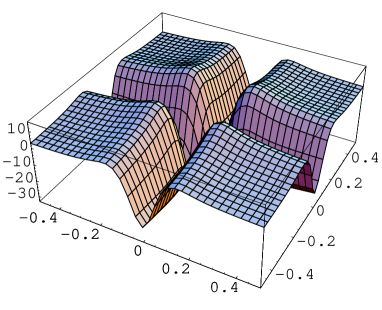
Figure 5: The Schrödinger potential $V(z_{1},z_{2})$ for the metric (11) with $k=1$ and $|z|\to z\,\tanh(10z)$.

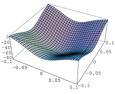
Figure 6: Close-up of the potential near the brane intersection.

5.1 A solvable example

In general, the Schrödinger equation (20) in the case of intersecting branes is fully $n$-dimensional and consequently rather complicated; however, in the case when

$$A(z)=\sum_{i=1}^{n}A^{(i)}(z^{i})\ ,$$ (98)

it is separable by writing $\psi(z)=\psi^{(1)}(z^{1})\times\cdots\times\psi^{(n)}(z^{n})$. In this case the solution represents $n$ intersecting $(d-2)$-branes where the intersection is four-dimensional.

For each $i$, $\psi^{(i)}(z^{i})$ satisfies a one-dimensional Schrödinger equation identical to (48) with $A(z)\to A^{(i)}(z^{i})$. Hence, we can immediately draw on the results of Sec. 4 to establish the conditions under which gravity is localized on the intersection. Basically we require that $\exp\big{[}-\tfrac{3}{2}A^{(i)}(z^{i})\big{]}$ falls off faster than $1/z^{i}$ as $|z^{i}|\to\infty$, for each $i$, so that the zero-energy state

$$\psi_{0}(z)=\psi^{(1)}_{0}(z^{1})\times\cdots\times\psi^{(n)}_{0}(z^{n})\ ,$$ (99)

is localized in all the transverse directions and therefore represents the four-dimensional graviton. In general, the spectrum consists of $2^{n}$ different sectors, depending on whether each $\psi^{(i)}(z^{i})$ is the normalizable wavefunction $\psi^{(i)}_{0}(z^{i})$ or a continuum wavefunction $\psi_{m}^{(i)}(z^{i})$. So for example, when there are 2 transverse directions there will be 4 sectors in the spectrum spanned by

(1) $$\psi_{0}^{(1)}(z^{1})\psi_{0}^{(2)}(z^{2})\ , \psi_{0}^{(1)}(z^{1})\psi_{m_{2}}^{(2)}(z^{2})\ ,$$ (2)

(3) $$\psi_{m_{1}}^{(1)}(z^{1})\psi_{0}^{(2)}(z^{2})\ , \psi_{m_{1}}^{(1)}(z^{1})\psi_{m_{2}}^{(2)}(z^{2})\ .$$ (4)

The first state (1) corresponds to the four-dimensional graviton. The set of continuum states (4) contributes to Newton’s Law as in (33),

$$\delta_{4}U(r)\thicksim M^{2-d}_{*}\int_{0}^{\infty}dm_{1}dm_{2}\,\frac{M_{1}M_{2}e^{-\sqrt{m_{1}^{2}+m_{2}^{2}}r}}{r}\psi_{m_{1}}^{(1)}(0)^{2}\psi_{m_{2}}^{(2)}(0)^{2}\ ,$$ (100)

The set of continuum states (2) or (3) are localized in one direction and contribute as an integral over the single eigenvalue $m_{2}$ and $m_{1}$, respectively,

$$\delta_{2+3}U(r)\thicksim M^{2-d}_{*}k\int_{0}^{\infty}dm_{1}\,\frac{M_{1}M_{2}e^{-m_{1}r}}{r}\psi_{m_{1}}^{(1)}(0)^{2}+M^{2-d}_{*}k\int_{0}^{\infty}dm_{2}\,\frac{M_{1}M_{2}e^{-m_{2}r}}{r}\psi_{m_{2}}^{(2)}(0)^{2}\ .$$ (101)

5.2 Intersecting branes from scalar fields

In this section, we consider whether the conformally-flat intersecting branes background can be generated from a single real scalar field. We argue that a single scalar field cannot produce a general intersecting brane background, but this leaves open the possibility that such backgrounds can be generated from more than one scalar field; for instance a single complex scalar as in [9]. In addition, we will also see, as promised in 4.5, that a single real scalar field cannot produce a conformally-flat three-brane embedded in $d>5$.

We assume the metric has the form (2), and there is a single scalar field which generates the energy-momentum tensor,

$$T_{\mu\nu}=\tfrac{1}{2}\partial_{\mu}\phi(z)\partial_{\nu}\phi(z)-\tfrac{1}{2}g_{\mu\nu}\big{(}\tfrac{1}{2}\partial^{\rho}\phi(z)\,\partial_{\rho}\phi(z)-{\cal V}[\phi(z)]\big{)}\ .$$ (102)

The Einstein tensor $G_{\mu\nu}$ can be read off of (13), and satisfies, for components transverse to the intersection,

$$G_{ii}=-G_{00}+\tfrac{d-2}{2}\big{[}\tfrac{1}{2}(\partial_{i}A(z))^{2}+\partial_{i}^{2}A(z)\big{]}\ .$$ (103)

The diagonal components of the stress tensor satisfy a similarly simple relation,

$$T_{ii}=-T_{00}+\big{(}\partial_{i}\,\phi(z)\big{)}^{2}\ ,$$ (104)

so the particular combination $G_{ii}+G_{00}=\kappa^{2}(T_{ii}+T_{00})$ of components of the Einstein equation relates derivatives of the scalar field to derivatives of the metric, independent of the form of the scalar potential ${\cal V}(\phi)$:

$$\tfrac{1}{2}\kappa^{2}\big{(}\partial_{i}\,\phi(z)\big{)}^{2}=\tfrac{d-2}{2}\big{[}\tfrac{1}{2}\partial_{i}A(z)\partial_{i}A(z)+\partial_{i}^{2}A(z)\big{]}\ .$$ (105)

The off-diagonal components of the Einstein equation are,

$$G_{ij}-\kappa^{2}T_{ij}=\tfrac{d-2}{2}\big{[}\tfrac{1}{2}\partial_{i}A(z)\partial_{j}A(z)+\partial_{i}\partial_{j}A(z)\big{]}-\tfrac{1}{2}\kappa^{2}\partial_{i}\phi(z)\partial_{j}\phi(z)=0\ ,$$ (106)

or, using (105),

$$\big{[}\partial_{i}\partial_{j}e^{A(z)/2}\big{]}^{2}=\big{[}\partial_{i}^{2}e^{A(z)/2}\big{]}\big{[}\partial_{j}^{2}e^{A(z)/2}\big{]}\ .$$ (107)

This constrains the type of metric which can be obtained by a gravitating scalar field. In particular, the solution of (107) is,

$$A(z)={\cal A}\big{(}\sum_{i=1}^{n}a_{i}\,z^{i}\big{)}\ ,$$ (108)

for some constant coefficients $a_{i}$. By a redefinition of coordinates, this can always be recast in the form $A(z)={\cal A}(z^{1})$, which preserves a $(d-1)$-dimensional Lorentz symmetry and hence can create only a single $(d-2)$-brane in $d$ dimensions. Therefore, it seems to be the case that additional fields are required to create intersecting branes in the presence of gravity. In addition, we conclude that a single real scalar field cannot produce a $p$-brane in $d>p+2$.

6 Conclusions

We have studied general features of gravity in domain wall backgrounds. For general domain wall type metrics we have found the conditions for there to be localized gravity on the domain wall or on the intersection of domain walls. It turns out that it is possible in generalizations of the Randall-Sundrum scenario for the graviton zero mode to be non-normalizable. It is precisely in that case that the effective gravitational coupling on the domain wall vanishes, and that the Kaluza-Klein modes become relevant at long distances. We have seen several illuminating examples in which smooth domain wall backgrounds are created by scalar fields, and in which the domain walls are created by non-dynamical sources in the absence of fields other than the graviton. Negative tension branes, such as appear in the RS solution to the hierarchy problem, can be studied in this formalism. We have studied intersecting domain walls in the absence of fields other than gravity, and we argued that a single scalar field is not sufficient to produce intersecting domain walls. We commented on resonant modes in the continuum of Kaluza-Klein modes, and argued that they are unimportant in smooth versions of the RS scenario.

One issue that is worth commenting on is the fate of the Lykken–Randall scenario for the solution of the hierarchy problem [12], in the context of thick branes. In this scenario we consider again the general five-dimensional backgrounds (47) but now associate the matter fields that describe our world with another brane—the “TeV brane”—located at a point $z_{0}$ in the transverse space. In order to create the necessary hierachy of scales we need $z_{0}$ such that

$$M_{\rm Pl}^{2}e^{-2A(z_{0})}\sim{\rm TeV}^{2}\ ,$$ (109)

where $M_{\rm Pl}$ is the Planck mass. In the context of the backgrounds discussed in Sec. 4, this requires that $z_{0}$ is much larger than $k$ (since $k\sim M_{\rm Pl}$). In other words, the TeV brane sits at a place where we may approximate the potential $V(z)$ by its asymptotic form (52). Since the relevant dynamics now takes place at $z=z_{0}$ we have to re-assess the effects of the KK modes. In particular, the effective Newton’s constant on the brane is now given by

$$G_{N}\sim\frac{M^{2-d}_{*}\hat{\psi}_{0}(z_{0})^{2}}{\langle\hat{\psi}_{0}|\hat{\psi}_{0}\rangle}\ .$$ (110)

This modifies the effects of the KK modes; in the case when the continuum starts at $m=0$, the corrections from the KK modes (33) are modified to [12]

$$U(r)\thicksim G_{N}\frac{M_{1}M_{2}}{r}\Big{[}1+\int_{0}^{\infty}dm\,\frac{M_{1}M_{2}e^{-mr}}{r}\Big{(}\frac{\psi_{m}(z_{0})}{\hat{\psi}_{0}(z_{0})}\Big{)}^{2}\Big{]}\ .$$ (111)

In the above, the zero-energy wavefunction $\hat{\psi}_{0}(z)$ must be normalized to unity $\langle\hat{\psi}_{0}|\hat{\psi}_{0}\rangle=1$. As $z_{0}$ increases then one might worry that the ratio $\psi_{m}(z_{0})/\hat{\psi}_{0}(z_{0})$ becomes larger and the effect of the KK modes is less suppressed and there would be large corrections to Newton’s Law. Actually, as explained in [12], this is not the case. Since $z_{0}$ lies in the tail of the potential (52), we can use the exact form of the solution in terms of Bessel functions (54) to assess the magnitude of the corrections. For small enough $m$ the first term in (54) dominates, and one finds using the expansion (57) (taking into account the correct normalizations on the wavefunctions)

$$\frac{\psi_{m}(z_{0})}{\hat{\psi}_{0}(z_{0})}\simeq\frac{\psi_{m}(0)}{\hat{\psi}_{0}(0)}\propto m^{\alpha-1}\ ,$$ (112)

and so the suppression is unchanged from the situation where matter fields are located at $z=0$. Small enough $m$ in this context means that we can approximate $\psi_{m}(z_{0})$ by the first term in (57).

The discussion above, where the matter fields are located at $z=z_{0}$ but are still point-like in the fifth dimension, also suggests that in a more realistic scenario, where the matter fields are smeared out in the fifth dimension, the corrections to Newton’s law will also be similarly suppressed and our previous insistence that the matter sources were point-like and located at $z=0$ was not overly simplistic.

- [1]
- [2] L. Randall and R. Sundrum, Phys. Rev. Lett. 83, 4690 (1999) [hep-th/9906064].
- [3] L. Randall and R. Sundrum, Phys. Rev. Lett. 83, 3370 (1999) [hep-ph/9905221].
- [4] V.A. Rubakov and M.E. Shaposhnikov, Phys. Lett. 125B, 139 (1983); M. Visser, Phys. Lett. 159B, 22 (1985); E.J. Squires, Phys. Lett. 167B, 286 (1986); G.W. Gibbons and D.L. Wiltshire, Nucl. Phys. B287, 717 (1987); M. Gogberashvili, hep-ph/9812296; hep-ph/9812365; hep-ph/9904383.
- [5] M. Gogberashvili, hep-ph/9908347.
- [6] N. Arkani-Hamed, S. Dimopoulos, G. Dvali and N. Kaloper, hep-th/9907209.
- [7] C. Csáki and Y. Shirman, Phys. Rev. D61, 024008 (2000) [hep-th/9908186].
- [8] A. E. Nelson, hep-th/9909001.
- [9] S. M. Carroll, S. Hellerman and M. Trodden, hep-th/9911083.
- [10] S. Nam, hep-th/9911104.
- [11] N. Kaloper, Phys. Rev. D60, 123506 (1999) [hep-th/9905210]; T. Nihei, Phys. Lett. B465, 81 (1999) [hep-ph/9905487]; H.B. Kim and H.D. Kim, hep-th/9909053.
- [12] J. Lykken and L. Randall, hep-th/9908076.
- [13] W. D. Goldberger and M. B. Wise, Phys. Rev. D60, 107505 (1999) [hep-ph/9907218].
- [14] W. D. Goldberger and M. B. Wise, Phys. Rev. Lett. 83, 4922 (1999) [hep-ph/9907447].
- [15] J. Cline, C. Grojean and G. Servant, hep-ph/9909496; C. Grojean, J. Cline and G. Servant, hep-th/9910081.
- [16] P. Kraus, JHEP 9912, 011 (1999) [hep-th/9910149]; A. Kehagias and E. Kiritsis, JHEP 9911, 022 (1999) [hep-th/9910174].
- [17] N. Kaloper, hep-th/9912125; S. Nam, hep-th/9911237.
- [18] L. Mersini, Mod. Phys. Lett. A14, 2393 (1999) [gr-qc/9906106]; hep-ph/9909494; hep-ph/0001017; E. Halyo, hep-th/9909127; J. Hisano and N. Okada, hep-ph/9909555; S. Chang, J. Hisano, H. Nakano, N. Okada and M. Yamaguchi, hep-ph/9912498; S. Chang and M. Yamaguchi, hep-ph/9909523; U. Ellwanger, hep-th/9909103; H. Hatanaka, M. Sakamoto, M. Tachibana and K. Takenaga, hep-th/9909076; I. Oda, hep-th/9909048; T. Li, hep-th/9908174; hep-th/9912182; H. Davoudiasl, J. L. Hewett and T. G. Rizzo, hep-ph/9911262; I. Oda, hep-th/9908104;
- [19] A. G. Cohen and D. B. Kaplan, hep-th/9910132.
- [20] A. Chodos and E. Poppitz, hep-th/9909199.
- [21] N. Arkani-Hamed, L. Hall, D. Smith and N. Weiner, hep-ph/9912453.
- [22] Z. Chacko and A.E. Nelson, hep-th/9912186.
- [23] I. I. Kogan, S. Mouslopoulos, A. Papazoglou, G. G. Ross and J. Santiago, hep-ph/9912552.
- [24] B. Bajc and G. Gabadadze, hep-th/9912232.
- [25] M. Chaichian and A. B. Kobakhidze, hep-th/9912193.
- [26] M. Cvetic, S. Griffies and S. Rey, Nucl. Phys. 381, 301 (1992) [hep-th/9201007]. For a review see: M. Cvetic and H.H. Soleng, Phys. Rept. 282, 159 (1997) [hep-th/9604090].
- [27] K. Behrndt and M. Cvetic, hep-th/9909058
- [28] O. DeWolfe, D.Z. Freedman, S.S. Gubser and A. Karch, hep-th/9909134.
- [29] A. Chamblin and G. W. Gibbons, hep-th/9909130.
- [30] M. Cvetic, H. Lu and C. N. Pope, hep-th/0001002; M. Cvetic and J. Wang, hep-th/9912187.
- [31] M. Gremm, hep-th/9912060.
- [32] A. Kehagias, Phys. Lett. B469, 123 (1999) [hep-th/9906204].
- [33] H. Verlinde, hep-th/9906182.
- [34] K. Skenderis and P. K. Townsend, Phys. Lett. B468, 46 (1999) [hep-th/9909070].
- [35] A. Brandhuber and K.Sfetsos, JHEP 9910, 013 (1999) [hep-th/9908116]; I. Bakas and K. Sfetsos, hep-th/9909041; I. Bakas, A. Brandhuber and K. Sfetsos, hep-th/9912132.
- [36] S.S. Gubser, hep-th/9912001.
- [37] D. Youm, hep-th/9911218; hep-th/9912175; hep-th/0001018.
- [38] R. Kallosh and A. Linde, hep-th/0001071.
- [39] A. Chamblin, S.W. Hawking and H.S. Reall, hep-th/9909205; J. Garriga and T. Tanaka, hep-th/9911055.
- [40] R. Emparan, G. Horowitz and R. Myers, hep-th/9911043; hep-th/9912135.
- [41] T. Shiromizu, K. Madea and M. Sasaki, gr-qc/9910076; hep-th/9912233; J. Garriga and M. Sasaki, hep-th/9912118; S. Mukohyama, T. Shiromizu and K. Maeda, hep-th/9912287.
- [42] I. Y. Aref’eva, hep-th/9910269
- [43] C. Charmousis, R. Gregory and V. Rubakov, hep-th/9912160.
- [44] M. G. Ivanov and I. V. Volovich, hep-th/9912242; S. Myung and G. Kang, hep-th/0001003.
- [45] J.E. Kim, B. Kyae, H.M. Lee, hep-ph/9912344.
- [46] A. Chamblin, D.M. Eardley, hep-th/9912166.
- [47] R. Dick and D. Mikulovicz, hep-th/0001013.
- [48] G. K. Leontaris and N. E. Mavromatos, hep-th/9912230.
- [49] C. Csáki, M. Graesser, C. Kolda and J. Terning, Phys. Lett. B462, 34 (1999) [hep-ph/9906513]; J. Cline, C. Grojean and G. Servant, Phys. Rev. Lett. 83, 4245 (1999)[hep-ph/9906523]; D. J. Chung and K. Freese, Phys. Rev. D61, 023511 (2000) [hep-ph/9906542]; P. Kanti, I.I. Kogan, K. Olive and M. Pospelov, Phys. Lett. B468, 31 (1999) [hep-ph/9909481]; hep-ph/9912266; C. Csáki, M. Graesser, L. Randall and J. Terning, hep-ph/9911406; W. Goldberger and M. Wise, hep-ph/9911457; D. N. Vollick, hep-th/9911181; D. Ida, gr-qc/9912002; D. J. Chung and K. Freese, hep-ph/9910235; A. Y. Neronov, gr-qc/9911122; S. Mukohyama, hep-th/9911165; L. Mersini, hep-ph/0001017.
- [50] E.E. Flanagan, S-H.H. Tye, I. Wasserman, hep-ph/9910498.
- [51] P. Binetruy, C. Deffayet and D. Langlois, hep-th/9905012; P. Binetruy, C. Deffayet, U. Ellwanger and D. Langlois, hep-th/9910219.
- [52] K.R. Dienes, E. Dudas and T. Gherghetta, hep-ph/9908530.
- [53] H. Davoudiasl, J.L. Hewett and T.G. Rizzo, hep-ph/9909255.
- [54] R. M. Wald, General Relativity, Univ. of Chicago Pr. (1984).
- [55]