PRA-HEP 99-07

1 Introduction

Parton distribution functions (PDF) are, together with the colour coupling $\alpha_{s}$, the basic ingredients of perturbative QCD calculations. It is worth emphasizing that in quantum field theory it is difficult to distinguish effects of the “structure” from those of “interactions”. Within the Standard Model (SM) it makes good sense to distinguish fundamental particles, which correspond to fields in its lagrangian ${\cal L}_{\mathrm{SM}}$ (leptons, quarks and gauge bosons) from composite particles, which appear in the mass spectrum but have no corresponding field in ${\cal L}_{\mathrm{SM}}$. For the latter the use of PDF to describe their “structure” appears natural, but the concept of PDF turns out to be phenomenologically useful also for some fundamental particles, in particular the photon. PDF are indispensable for the real photon due to strong interactions between the $q\overline{q}$ pair to which it couples electromagnetically. For massless quarks this coupling leads to singularities, which must be absorbed in PDF of the photon, similarly as in the case of hadrons. Although PDF of the real photon satisfy inhomogeneous evolution equations, their physical meaning remains basically the same as for hadrons.

For nonzero photon virtualities there is no true singularity associated with the coupling $\gamma^{*}\rightarrow q\overline{q}$ and one therefore expects that for sufficiently virtual photon its interactions should be calculable perturbatively, with no need to introduce PDF. The main aim of this paper is to advocate the use of PDF also for virtual photons involved in hard collisions.

Throughout this paper we shall stay within the conventional approach to evolution equations for PDF of the photon. The reformulation of the whole framework for the description of hard collisions involving photons in the initial state, proposed recently by one of us [1], affects the analysis of dijet production in photon–proton collisions, which is the main subject of this paper, only marginally. This stands in sharp contrast to QCD analysis of $F_{2}^{\gamma}$ which is affected by this reformulation quite significantly.

The paper is organized as follows. In Section 2 the notation and basic facts concerning the evolution equations for PDF of the real photon and the properties of their solutions are recalled. In Section 3 the physical content of PDF of the virtual photon is analyzed and its phenomenological relevance illustrated within the LO QCD. This is further underlined in Section 4 by detailed analysis of NLO QCD calculations of dijet cross–sections in ep collisions, followed by the summary and conclusions in Section 5.

2 PDF of the real photon

In QCD the coupling of quarks and gluons is characterized by the renormalized colour coupling (“couplant” for short) $\alpha_{s}(\mu)$, depending on the renormalization scale $\mu$ and satisfying the equation

$$\frac{{\mathrm{d}}\alpha_{s}(\mu)}{{\mathrm{d}}\ln\mu^{2}}\equiv\beta(\alpha_{s}(\mu))=-\frac{\beta_{0}}{4\pi}\alpha_{s}^{2}(\mu)-\frac{\beta_{1}}{16\pi^{2}}\alpha_{s}^{3}(\mu)+\cdots,$$ (1)

where, in QCD with $n_{f}$ massless quark flavours, the first two coefficients, $\beta_{0}=11-2n_{f}/3$ and $\beta_{1}=102-38n_{f}/3$, are unique, while all the higher order ones are ambiguous. As we shall stay in this paper within the NLO QCD, only the first two, unique, terms in (1) will be taken into account. However, even for a given r.h.s. of (1) its solution $\alpha_{s}(\mu)$ is not a unique function of $\mu$, because there is an infinite number of solutions of (1), differing by the initial condition. This so called renormalization scheme (RS) ambiguity can be parameterized in a number of ways. One of them makes use of the fact that in the process of renormalization another dimensional parameter, denoted usually $\Lambda$, inevitably appears in the theory. This parameter depends on the RS and at the NLO even fully specifies it. For instance, $\alpha_{s}(\mu)$ in the familiar MS and $\overline{\mathrm{MS}}$ RS are two solutions of the same equation (1), associated with different $\Lambda_{\mathrm{RS}}$. At the NLO the variation of both the renormalization scale $\mu$ and the renormalization scheme RS$\equiv${$\Lambda_{\mathrm{RS}}$} is redundant. It suffices to fix one of them and vary the other, but we stick to the common practice of considering both of them as free parameters. In this paper we shall work in the standard $\overline{\mathrm{MS}}$ RS of the couplant.

The “dressed” PDF result from the resummation of multiple parton collinear emission off the corresponding “bare” parton distributions. As a result of this resummation PDF acquire dependence on the factorization scale $M$. This scale defines the upper limit on some measure $t$ of the off–shellness of partons included in the definition of $D(x,M)$

$$D_{i}(x,M)\equiv\int_{t_{\mathrm{min}}}^{M^{2}}{\mathrm{d}}td_{i}(x,t),~{}~{}~{}~{}~{}~{}i=q,\overline{q},G,$$ (2)

where the unintegrated PDF $d_{i}(x,t)$ describe distributions of partons with the momentum fraction $x$ and fixed off–shellness $t$. Parton virtuality $\tau\equiv\mid p^{2}-m^{2}\mid$ or transverse mass $m_{T}^{2}\equiv p_{T}^{2}+m^{2}$, are two standard choices of such a measure. Factorization scale dependence of PDF of the photon is determined by the system of coupled inhomogeneous evolution equations

$$\frac{{\mathrm{d}}\Sigma(x,M)}{{\mathrm{d}}\ln M^{2}} = \delta_{\Sigma}k_{q}+P_{qq}\otimes\Sigma+P_{qG}\otimes G,$$ (3)

$$\frac{{\mathrm{d}}G(x,M)}{{\mathrm{d}}\ln M^{2}} = k_{G}+P_{Gq}\otimes\Sigma+P_{GG}\otimes G,$$ (4)

$$\frac{{\mathrm{d}}q_{\mathrm{NS}}(x,M)}{{\mathrm{d}}\ln M^{2}} = \delta_{\mathrm{NS}}k_{q}+P_{\mathrm{NS}}\otimes q_{\mathrm{NS}},$$ (5)

where

$$\Sigma(x,M) \equiv \sum_{i=1}^{n_{f}}q_{i}^{+}(x,M)\equiv\sum_{i=1}^{n_{f}}\left[q_{i}(x,M)+\overline{q}_{i}(x,M)\right],$$ (6)

$$q_{\mathrm{NS}}(x,M) \equiv \sum_{i=1}^{n_{f}}\left(e_{i}^{2}-\langle e^{2}\rangle\right)\left(q_{i}(x,M)+\overline{q}_{i}(x,M)\right),$$ (7)

$$\delta_{\mathrm{NS}}=6n_{f}\left(\langle e^{4}\rangle-\langle e^{2}\rangle^{2}\right),~{}~{}~{}\delta_{\Sigma}=6n_{f}\langle e^{2}\rangle.$$ (8)

To order $\alpha$ the splitting functions $P_{ij}$ and $k_{i}$ are given as power expansions in $\alpha_{s}(M)$:

$$k_{q}(x,M) = \frac{\alpha}{2\pi}\left[k^{(0)}_{q}(x)+\frac{\alpha_{s}(M)}{2\pi}k_{q}^{(1)}(x)+\left(\frac{\alpha_{s}(M)}{2\pi}\right)^{2}k^{(2)}_{q}(x)+\cdots\right],$$ (9)

$$k_{G}(x,M) = \frac{\alpha}{2\pi}\left[~{}~{}~{}~{}~{}~{}~{}~{}~{}~{}~{}~{}\frac{\alpha_{s}(M)}{2\pi}k_{G}^{(1)}(x)+\left(\frac{\alpha_{s}(M)}{2\pi}\right)^{2}k^{(2)}_{G}(x)+\cdots\;\right],$$ (10)

$$P_{ij}(x,M) = ~{}~{}~{}~{}~{}~{}~{}~{}~{}~{}~{}~{}~{}~{}~{}~{}~{}~{}\frac{\alpha_{s}(M)}{2\pi}P^{(0)}_{ij}(x)+\left(\frac{\alpha_{s}(M)}{2\pi}\right)^{2}P_{ij}^{(1)}(x)+\cdots,$$ (11)

where the leading order splitting functions $k_{q}^{(0)}(x)=x^{2}+(1-x)^{2}$ and $P^{(0)}_{ij}(x)$ are unique, while all higher order ones $k^{(j)}_{q},k^{(j)}_{G},P^{(j)}_{kl},j\geq 1$ depend on the choice of the factorization scheme (FS). The equations (3-5) can be rewritten as evolution equations for $q_{i}(x,M),\overline{q}_{i}(x,M)$ and $G(x,M)$ with inhomegenous splitting functions $k_{q_{i}}^{(0)}=3e_{i}^{2}k_{q}^{(0)}$. The photon structure function $F_{2}^{\gamma}(x,Q^{2})$, measured in deep inelastic scattering of electrons on photons is given as a sum of convolutions

$$\frac{1}{x}F_{2}^{\gamma}(x,Q^{2}) = q_{\mathrm{NS}}(M)\otimes C_{q}(Q/M)+\frac{\alpha}{2\pi}\delta_{\mathrm{NS}}C_{\gamma}+$$ (13)

$$\langle e^{2}\rangle\Sigma(M)\otimes C_{q}(Q/M)+\frac{\alpha}{2\pi}\langle e^{2}\rangle\delta_{\Sigma}C_{\gamma}+\langle e^{2}\rangle\frac{\alpha_{s}}{2\pi}G(M)\otimes C_{G}(Q/M)$$

of photonic PDF and coefficient functions $C_{q}(x),C_{G}(x),C_{\gamma}(x)$ admitting perturbative expansions

$$C_{q}(x,Q/M) = \delta(1-x)~{}~{}~{}~{}+~{}~{}~{}\frac{\alpha_{s}(\mu)}{2\pi}C^{(1)}_{q}(x,Q/M)+\cdots,$$ (14)

$$C_{G}(x,Q/M) = ~{}~{}~{}~{}~{}~{}~{}~{}~{}~{}~{}~{}~{}~{}~{}~{}~{}~{}~{}~{}~{}\frac{\alpha_{s}(\mu)}{2\pi}C^{(1)}_{G}(x,Q/M)+\cdots,$$ (15)

$$C_{\gamma}(x,Q/M) = C_{\gamma}^{(0)}(x,Q/M)+\frac{\alpha_{s}(\mu)}{2\pi}C_{\gamma}^{(1)}(x,Q/M)+\cdots.$$ (16)

The renormalization scale $\mu$, used as argument of $\alpha_{s}(\mu)$ in (14-16) is in principle independent of the factorization scale $M$. Note that despite the presence of $\mu$ as argument of $\alpha_{s}(\mu)$ in (14–16), the coefficient functions $C_{q},C_{G}$ and $C_{\gamma}$, summed to all orders of $\alpha_{s}$, are actually independent of it, because the $\mu$–dependence of the expansion parameter $\alpha_{s}(\mu)$ is cancelled by explicit dependence of $C^{(i)}_{q},C^{(i)}_{G},C^{(i)}_{\gamma},i\geq 2$ on $\mu$. On the other hand, PDF as well as the coefficient functions $C_{q},C_{G}$ and $C_{\gamma}$ do depend on both the factorization scale $M$ and factorization scheme, but in such a correlated manner that physical quantities, like $F_{2}^{\gamma}$, are independent of both $M$ and the FS, provided expansions (9–11) and (14–16) are taken to all orders in $\alpha_{s}(M)$ and $\alpha_{s}(\mu)$. In practical calculations based on truncated forms of (9–11) and (14–16) this invariance is, however, lost and the choice of both $M$ and FS makes numerical difference even for physical quantities. The expressions for $C_{q}^{(1)},C^{(1)}_{G}$ given in [2] are usually claimed to correspond to “$\overline{\mathrm{MS}}$ factorization scheme”. As argued in [3], this denomination is, however, incomplete. The adjective “$\overline{\mathrm{MS}}$” concerns exclusively the choice of the RS of the couplant $\alpha_{s}$ and has nothing to do with the choice of the splitting functions $P^{(1)}_{ij}$. The choices of the renormalization scheme of the couplant $\alpha_{s}$ and of the factorization scheme of PDF are two completely independent decisions, concerning two different and in general unrelated redefinition procedures. Both are necessary in order to specify uniquely the results of fixed order perturbative calculations, but we may combine any choice of the RS of the couplant with any choice of the FS of PDF. The coefficient functions $C_{q},C_{G},C_{\gamma}$ depend on both of them, whereas the splitting functions depend only on the latter. The results given in [2] correspond to $\overline{\mathrm{MS}}$ RS of the couplant but to the “minimal subtraction” FS of PDF . It is therefore more appropriate to call this full specification of the renormalization and factorization schemes as “$\overline{\mathrm{MS}}+{\mathrm{MS}}$ scheme”. Although the phenomenological relevance of treating $\mu$ and $M$ as independent parameters has been demonstrated [5], we shall follow the usual practice of setting $\mu=M$.

2.1 Pointlike solutions and their properties

The general solution of the evolution equations (3-5) can be written as the sum of a particular solution of the full inhomogeneous equation and the general solution of the corresponding homogeneous one, called hadronic part. A subset of the solutions of full evolution equations resulting from the resummation of series of diagrams like those in Fig. 1, which start with the pointlike purely QED vertex $\gamma\rightarrow q\overline{q}$, are called pointlike (PL) solutions. In writing down the expression for the resummation of diagrams in Fig. 1 there is a freedom in specifying some sort of boundary condition. It is common to work within a subset of pointlike solutions specified by the value of the scale $M_{0}$ at which they vanish. In general, we can thus write ($D=q,\overline{q},G$)

$$D(x,M^{2})=D^{\mathrm{PL}}(x,M^{2})+D^{\mathrm{HAD}}(x,M^{2}).$$ (17)

Due to the fact that there is an infinite number of pointlike solutions $q^{\mathrm{PL}}(x,M^{2})$, the separation of quark and gluon distribution functions into their pointlike and hadronic parts is, however, ambiguous and therefore these concepts have separately no physical meaning. In [6] we discussed numerical aspects of this ambiguity for the Schuler–Sjöstrand sets of parameterizations [7].

Figure 1: Diagrams defining the pointlike parts of nonsinglet quark and gluon distribution functions. The resummation involves integration over parton virtualities $\tau\leq M^{2}$.

To see the most important feature of the pointlike part of quark distribution functions that will be crucial for the following analysis, let us consider in detail the case of nonsinglet quark distribution function $q_{\mathrm{NS}}(x,M)$, which is explicitly defined via the series

$$q^{\mathrm{PL}}_{\mathrm{NS}}(x,M_{0},M)\equiv\frac{\alpha}{2\pi}k_{\mathrm{NS}}^{(0)}(x)\int^{M^{2}}_{M_{0}^{2}}\frac{{\mathrm{d}}\tau}{\tau}+\int^{1}_{x}\frac{{\mathrm{d}}y}{y}P^{(0)}_{qq}\left(\frac{x}{y}\right)\int^{M^{2}}_{M_{0}^{2}}\frac{{\mathrm{d}}\tau_{1}}{\tau_{1}}\frac{\alpha_{s}(\tau_{1})}{2\pi}\frac{\alpha}{2\pi}k_{\mathrm{NS}}^{(0)}(y)\int^{\tau_{1}}_{M_{0}^{2}}\frac{{\mathrm{d}}\tau_{2}}{\tau_{2}}+$$

$$\int^{1}_{x}\frac{{\mathrm{d}}y}{y}P^{(0)}_{qq}\left(\frac{x}{y}\right)\int^{1}_{y}\frac{{\mathrm{d}}w}{w}P^{(0)}_{qq}\left(\frac{y}{w}\right)\int^{M^{2}}_{M_{0}^{2}}\frac{{\mathrm{d}}\tau_{1}}{\tau_{1}}\frac{\alpha_{s}(\tau_{1})}{2\pi}\int^{\tau_{1}}_{M_{0}^{2}}\frac{{\mathrm{d}}\tau_{2}}{\tau_{2}}\frac{\alpha_{s}(\tau_{2})}{2\pi}\frac{\alpha}{2\pi}k_{\mathrm{NS}}^{(0)}(w)\int^{\tau_{2}}_{M_{0}^{2}}\frac{{\mathrm{d}}\tau_{3}}{\tau_{3}}+\cdots,$$ (18)

where $k_{\mathrm{NS}}^{(0)}(x)=\delta_{\mathrm{NS}}k^{(0)}_{q}(x)$. In terms of moments defined as

$$f(n)\equiv\int_{0}^{1}x^{n}f(x)\mathrm{d}x$$ (19)

this series can be resummed in a closed form

$$q_{\mathrm{NS}}^{\mathrm{PL}}(n,M_{0},M)=\frac{4\pi}{\alpha_{s}(M)}\left[1-\left(\frac{\alpha_{s}(M)}{\alpha_{s}(M_{0})}\right)^{1-2P^{(0)}_{qq}(n)/\beta_{0}}\right]a_{\mathrm{NS}}(n),$$ (20)

where

$$a_{\mathrm{NS}}(n)\equiv\frac{\alpha}{2\pi\beta_{0}}\frac{k_{\mathrm{NS}}^{(0)}(n)}{1-2P^{(0)}_{qq}(n)/\beta_{0}}.$$ (21)

Figure 2: Comparison, left in the nonsinglet and right in the singlet channels, of the functions $xk_{i}(x)=x\delta_{i}k_{q}^{(0)},i=\mathrm{NS},\Sigma$ with the function (21) and its analogue in the singlet channel.

It is straightforward to show that (18) or, equivalently, (20), satisfy the evolution equation (5) with the splitting functions $k_{q}$ and $P_{ij}$ including the first terms $k_{q}^{(0)}$ and $P_{qq}^{(0)}$ only.

Transforming (21) to the $x$–space by means of inverse Mellin transformation we get $a_{\mathrm{NS}}(x)$ shown in Fig. 2. The resummation softens the $x-$dependence of $a_{\mathrm{NS}}(x)$ with respect to the first term in (18), proportional to $k_{\mathrm{NS}}(x)$, but does not change the logarithmic dependence of $q_{\mathrm{NS}}$ on $M$. In the nonsinglet channel the effects of gluon radiation on $q_{\mathrm{NS}}^{\mathrm{PL}}$ are significant for $x>0.6$ but small elsewhere, whereas in the singlet channel such effects are marked also for $x<0.5$ and lead to a steep rise of $xq_{\mathrm{NS}}^{\mathrm{PL}}$ at very small $x$. As emphasized long time ago by authors of [8] the logarithmic dependence of $q_{\mathrm{NS}}^{\mathrm{PL}}$ on $\ln M$ has nothing to do with QCD and results exclusively from integration over the transverse momenta (virtualities) of quarks coming from the basic QED $\gamma^{*}\rightarrow q\overline{q}$ splitting. For $M/M_{0}\rightarrow\infty$ the second term in brackets of (20) vanishes and therefore all pointlike solutions share the same large $M$ behaviour

$$q^{\mathrm{PL}}_{\mathrm{NS}}(x,M_{0},M)\rightarrow\frac{4\pi}{\alpha_{s}(M)}a_{\mathrm{NS}}(x)\equiv q^{\mathrm{AP}}_{\mathrm{NS}}(x,M)\propto\ln\frac{M^{2}}{\Lambda^{2}},$$ (22)

defining the so called asymptotic pointlike solution $q^{\mathrm{AP}}_{\mathrm{NS}}(x,M)$ [9, 10]. The fact that for the asymptotic pointlike solution (22) $\alpha_{s}(M)$ appears in the denominator of (22) has been the source of misleading claims that $q(x,M)=O(\alpha/\alpha_{s})$. In fact, as argued in detail in [1], $q(x,M)=O(\alpha)$ as suggested by explicit construction in (18). We shall return to this point in Section 4.2 when discussing the factorization scale invariance of finite order approximations to dijet cross–sections.

The arbitrariness in the choice of $M_{0}$ reflects the fact that as $M_{0}$ increases, less of the gluon radiation effects is included in the resummation (20) defining the pointlike part of quark distribution function $q^{\mathrm{PL}}$ but included in hadronic one. The latter is usually modelled by the VDM ansatz and will therefore be called “VDM” in the following. As we shall see, the hadronic and pointlike parts have very different behaviour as functions of $x$ and $M$.

2.2 Properties of Schuler–Sjöstrand parameterizations

Practical aspects of the ambiguity in separating PDF into their VDM and pointlike parts can be illustrated on the properties of SaS1D and SaS2D parameterizations [7] . What makes the SaS approach particularly useful for our discussion is the fact that it provides separate parameterizations of the VDM and pointlike parts of both quark and gluon distributions.

Figure 3: The $u$ and $c$ quark and gluon distribution functions of the real photon for SaS1D (upper solid curves) and SaS2D (upper dotted curves) parameterizations at $M^{2}=100$ GeV². The VDM and pointlike parts of both parameterizations are plotted separately, the latter as solid and dotted curves peaking at large $x$. For quarks the splitting terms (23) corresponding to SaS1D and SaS2D (upper and lower dashed curves) are overlayed to show the effects of resummation (18).

Figure 4: Factorization scale dependence of parton distributions functions $u(x,M),c(x,M)$ and $G(x,M)$ of the real photon. Dashed and solid curves correspond, in the order indicated by the arrows, to pointlike and VDM parts of these distributions at $M^{2}=25,100$ and $1000$ GeV². In the lower part SaS1D quark distribution functions $xu(x,M^{2},P^{2})$ rescaled by $\ln(M^{2}/M_{0}^{2})$ for the real photon (left) and by $\ln(M^{2}/P^{2})$ for the virtual one, are plotted and compared to the predictions of the splitting term (23).

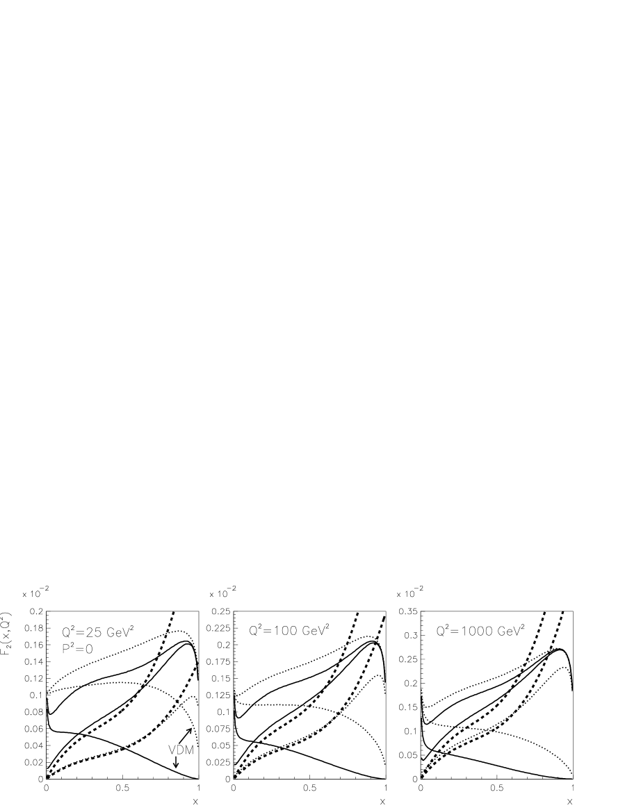
Figure 5: $F_{2}^{\gamma}(x,Q^{2})$ as given by SaS1D (solid curves) and SaSD2 (dotted curves) parameterizations. The full results are given by the upper, the pointlike and VDM contributions parts by two lower curves. The dashed curves describe the contributions of the splitting term (23).

Figure 6: $D_{\mathrm{e}ff}(x,M^{2})$ as given by SaS1D and SaSD2 parameterizations. Solid curves show the full results, dashed ones the VDM contributions. The pointlike parts are separated into the contributions of pointlike quarks (dotted curves) and pointlike gluons (dash–dotted). Thick dashed curves correspond to the splitting term (23).

In Fig. 3 distribution functions $xu(x,M^{2})$, $xc(x,M^{2})$ and $xG(x,M^{2})$ as given by SaS1D and SaS2D parameterizations for $M^{2}=100$ GeV² are compared. To see how much the resummation of gluon radiation modifies the first term in (18) we also plot the corresponding splitting terms

$$q^{\mathrm{s}plit}(x,M_{0}^{2},M^{2})\equiv\frac{\alpha}{2\pi}3e_{q}^{2}\left(x^{2}+(1-x)^{2}\right)\ln\frac{M^{2}}{M_{0}^{2}}.$$ (23)

In Fig. 4 the scale dependence of VDM and pointlike parts of $u$ and $c$ quark and gluon distribution functions is displayed. In the upper six plots we compare them as a function of $x$ at $M^{2}=25,100,1000$ GeV², while in the lower three plots the same distributions are rescaled by the factor $\ln(M^{2}/M_{0}^{2})$. Dividing out this dominant scale dependence allows us to compare the results directly to curves in Fig. 2. Finally, in Figs. 5 and 6 SaS predictions for two physical quantities, $F_{2}^{\gamma}$ and effective parton distribution function $D_{\mathrm{eff}}$, relevant for jet production in $\gamma$p and $\gamma\gamma$ collisions,

$$F_{2}^{\gamma}(x,Q^{2}) = \sum_{q}2xe_{q}^{2}q(x,Q^{2}),$$ (24)

$$D_{\mathrm{e}ff}(x,M^{2}) \equiv \sum_{i=1}^{n_{f}}\left(q_{i}(x,M^{2})+\overline{q}_{i}(x,M^{2})\right)+\frac{9}{4}G(x,M^{2})$$ (25)

are displayed and compared to results corresponding to the splitting term (23). Figures 3–6 illustrate several important properties of PDF of the real photon:

• There is a huge difference between the importance of the VDM components of light quark and gluon distribution functions in SaS1D and SaS2D parameterizations: while for SaS2D the VDM component is dominant up to $x\doteq 0.75$, for SaS1D the pointlike one takes over above $x\doteq 0.1$!

• Factorization scale dependence of VDM and pointlike parts differ substantially. While the former exhibits the pattern of scaling violations typical for hadrons, the latter rises, for quarks as well as gluons, with $M$ for all $x$. For pointlike gluons this holds despite the fact that $G^{\mathrm{PL}}(x,M^{2})$ satisfies at the LO standard homogeneous evolution equation and is due to the fact that the evolution of $G^{\mathrm{PL}}(x,M^{2})$ is driven by the corresponding increase of $\Sigma^{\mathrm{PL}}(x,M^{2})$.

• The approach of $q^{\mathrm{PL}}(x,M^{2})$ to the asymptotic pointlike solution (22) is slow . For experimentally relevant values of $M$ and except for $x$ close to $1$ the effects of multiple gluon emission on pointlike quarks are thus small.

• As the factorization scale $M$ increases the VDM parts of both quark and gluon distribution functions decrease relative to the pointlike ones, except in the region of very small $x$.

• Despite huge differences between SaS1D and SaS2D parameterizations in the decomposition of quark and gluon distributions into their VDM and pointlike parts, their predictions for physical observables $F_{2}^{\gamma}$ and $D_{\mathrm{eff}}$ are much closer.

• The most prominent effects of multiple parton emission on physical quantities appear to be the behaviour of $F_{2}^{\gamma}(x,Q^{2})$ at large $x$ and the contribution of pointlike gluons to jet cross–sections, approximately described by $D_{\mathrm{eff}}(x,M^{2})$.

3 PDF of the virtual photon

For the virtual photon the initial state singularity due to the splitting $\gamma^{*}\rightarrow q\overline{q}$ is shielded off by the nonzero initial photon virtuality $P^{2}$ and therefore in principle the concept of PDF does not have to be introduced. In practice this requires, roughly, $P^{2}>1$ GeV², where perturbative QCD becomes applicable. Nevertheless, PDF still turn out to be phenomenologically very useful because

• their pointlike parts include the resummation of parts of higher order QCD corrections,

• the hadronic parts, though decreasing rapidly with $P^{2}$, are still vital at very small $x$.

Both of these aspects define the “nontrivial” structure of the virtual photon in the sense that they are not included in the splitting term (23) and thus are not part of existing NLO unsubtracted direct photon calculations. One might argue that the calculable effects of resummation should be considered as “interaction” rather than “structure”, but their uniqueness makes it natural to describe them in terms of PDF.

3.1 Equivalent photon approximation

All the present knowledge of the structure of the photon comes from experiments at the ep and e⁺e^- colliders, where the incoming leptons act as sources of transverse and longitudinal virtual photons. To order $\alpha$ their respective unintegrated fluxes are given as

$$f^{\gamma}_{T}(y,P^{2}) = \frac{\alpha}{2\pi}\left(\frac{1+(1-y)^{2})}{y}\frac{1}{P^{2}}-\frac{2m_{\mathrm{e}}^{2}y}{P^{4}}\right),$$ (26)

$$f^{\gamma}_{L}(y,P^{2}) = \frac{\alpha}{2\pi}\frac{2(1-y)}{y}\frac{1}{P^{2}}.$$ (27)

The transverse and longitudinal fluxes thus coincide at $y=0$, while at $y=1$, $f_{L}^{\gamma}$ vanishes. The $1/P^{2}$ dependence of the first terms in (26-27) results from the fact that in both cases the vertex where photon is emitted is proportional to $P^{2}$. This is due to helicity conservation for the transverse photon and gauge invariance for the longitudinal one. The term proportional to $m_{\mathrm{e}}^{2}/P^{4}$ in (26) results from the fact that the helicity conservation at the e$\gamma$e vertex is violated by terms proportional to electron mass. No such violation is permitted in the case of gauge invariance, hence the absence of such term in (27). Note that while for $P^{2}\gg m_{\mathrm{e}}^{2}$ the second term in (26) is negligible with respect to the leading $1/P^{2}$ one, close to $P^{2}_{\mathrm{m}in}=m_{e}^{2}y^{2}/(1-y)$ their ratio is finite and approaches $2(1-y)/(1+(1-y)^{2})$.

3.2 Lessons from QED

The definition and evaluation of quark distribution functions of the virtual photon in pure QED serves as a useful guide to parton model predictions of virtuality dependence of the pointlike part of quark distribution functions of the virtual photon. In pure QED and to order $\alpha$ the probability of finding inside the photon of virtuality $P^{2}$ a quark with mass $m_{q}$, electric charge $e_{q}$, momentum fraction $x$ and virtuality $\tau=m_{q}^{2}-k^{2}\leq M^{2}$ is defined as ($k$ denotes its four-momentum)

$$q_{\mathrm{QED}}(x,m^{2}_{q},P^{2},M^{2})\equiv\left(\frac{\alpha}{2\pi}3e_{q}^{2}\right)\int_{\tau^{\mathrm{min}}}^{M^{2}}\frac{W(x,m^{2}_{q},P^{2})}{\tau^{2}}{\mathrm{d}}\tau,$$ (28)

where the function $W(x,m_{q}^{2},P^{2},M^{2})$ can in general be written as

$$W(x,m^{2}_{q},P^{2},M^{2}) = f(x)\frac{p_{T}^{2}}{1-x}+g(x)m^{2}_{q}+h(x)P^{2}+\cdots$$ (29)

$$= f(x)\tau+\left(g(x)-\frac{f(x)}{1-x}\right)m^{2}_{q}+\left(h(x)-xf(x)\right)P^{2}+\cdots.$$

In the collinear kinematics, which is relevant for finding the lower limit on $\tau$, the values of $m_{q},~{}x,~{}\tau$ and $p_{T}$ are related to initial photon virtuality $P^{2}$ as follows

$$\tau=xP^{2}+\frac{m_{q}^{2}+p_{T}^{2}}{1-x},~{}~{}~{}\Rightarrow~{}~{}~{}\tau^{\mathrm{min}}=xP^{2}+\frac{m_{q}^{2}}{1-x}.$$ (30)

The functions $f(x),g(x)$ and $h(x)$, which determine the terms singular at small $\tau$, are unique functions that have a clear parton model interpretation: so long as $\tau\ll M^{2}$ eq. (28) describes the flux of quarks that are almost collinear with the incoming photon and “live” long with respect to $1/M$. On the other hand, the terms indicated in (29) by dots are of the type $\tau^{k+1}/s^{k},k\geq 1$, which upon insertion into (28) yield contributions that are not singular at $\tau=0$ and therefore do not admit simple parton model interpretation. In principle we can include in the definition (28) even part of these nonpartonic contributions, but we prefer not do that. Substituting (29) into (28) and performing the integration gives, in units of $3e_{q}^{2}\alpha/2\pi$,

$$q_{\mathrm{QED}}(x,m_{q}^{2},P^{2},M^{2})=f(x)\ln\left(\frac{M^{2}}{\tau^{\mathrm{min}}}\right)+\left[-f(x)+\frac{g(x)m_{q}^{2}+h(x)P^{2}}{\tau^{\mathrm{min}}}\right]\left(1-\frac{\tau^{\mathrm{min}}}{M^{2}}\right).$$ (31)

In practical applications the factorization scale M is identified with some kinematical variable characterizing hardness of the collision, like $\sqrt{Q^{2}}$ in DIS or $E_{T}^{\mathrm{j}et}$ in jet production. For $\tau^{\mathrm{min}}\ll M^{2}$ the expression (31) simplifies to

$$q_{\mathrm{QED}}(x,m_{q}^{2},P^{2},M^{2})=f(x)\ln\left(\frac{M^{2}}{xP^{2}+m_{q}^{2}/(1-x)}\right)-f(x)+\frac{g(x)m_{q}^{2}+h(x)P^{2}}{xP^{2}+m_{q}^{2}/(1-x)}.$$ (32)

For $x(1-x)P^{2}\gg m_{q}^{2}$ this expression reduces further to

$$q_{\mathrm{QED}}(x,0,P^{2},M^{2})=f(x)\ln\left(\frac{M^{2}}{xP^{2}}\right)-f(x)+\frac{h(x)}{x}.$$ (33)

Provided $m_{q}^{2}\neq 0$ (32) has a finite limit for $P^{2}\rightarrow 0$, corresponding to the real photon

$$q_{\mathrm{QED}}(x,m_{q}^{2},0,M^{2})=f(x)\ln\left(\frac{M^{2}(1-x)}{m_{q}^{2}}\right)-f(x)+g(x)(1-x).$$ (34)

As in the case of the photon fluxes (26-27) the logarithmic term, dominant for large $M^{2}$, as well as the “constant” terms, proportional to $f(x),g(x)$ and $h(x)$, come entirely from the integration region close to $\tau^{\mathrm{min}}$ and are therefore unique. At $\tau=\tau^{\mathrm{min}}$ both types of the singular terms, i.e. $1/\tau$ or $1/\tau^{2}$, are of the same order but the faster fall–off of the $1/\tau^{2}$ terms implies that for large $M^{2}$ the integral over $\tau$, which gives (31), is dominated by the weaker singularity $1/\tau$. In other words, while the logarithmic term is dominant at large $M^{2}$, the constant terms resulting from nonzero $m^{2}$ and $P^{2}$ come from the kinematical configurations which are even more collinear, and thus more partonic, than those giving the logarithmic term. The analysis of the vertex $\gamma^{*}\rightarrow q\overline{q}$ in collinear kinematics yields [12]

$$\begin{array}[]{lll}f_{T}(x)=x^{2}+(1-x)^{2},&g_{T}(x)={\displaystyle\frac{\displaystyle 1}{\displaystyle 1-x}},&h_{T}(x)=0,\\[11.38092pt] f_{L}(x)=0,&g_{L}(x)=0,&h_{L}(x)=4x^{2}(1-x).\end{array}$$ (35)

The expressions (31-32) exhibit explicitly the smooth transition between quark distribution functions of the virtual and real photon. This transition is governed by the ratio $P^{2}/m^{2}$, which underlines why in QED fermion masses are vital. On the other hand, as $P^{2}$ (or more precisely $\tau^{\mathrm{m}in}$) increases toward the factorization scale $M^{2}$, the above expressions for the quark distribution functions of the virtual photon vanish. This property holds not only for the logarithmic term but also for the “constant” terms and has a clear intuitive content: virtual photon with lifetime $1/P\ll 1/M$ does not contain partons living long enough to take part in the collision characterized by the interaction time $1/M$.

For virtual photon and $x(1-x)P^{2}\gg m^{2}$ the coefficient functions $C_{\gamma}^{T}(x,P^{2},Q/M),C_{\gamma}^{L}(x,P^{2},Q/M)$ for transverse and longitudinal target photon polarizations are given as [13]

$$C_{\gamma,T}^{(0)}(x,P^{2},1) = 3\left[(x^{2}+(1-x)^{2})\ln\frac{1}{x^{2}}+8x(1-x)-2\right],$$ (36)

$$C_{\gamma,L}^{(0)}(x,P^{2},1) = 4x(1-x),$$ (37)

whereas for the real photon, i.e. for $P^{2}=0$

$$C_{\gamma,T}^{(0)}(x,0,1) = 3\left[(x^{2}+(1-x)^{2})\ln\frac{1-x}{x}+8x(1-x)-1\right],$$ (38)

$$C_{\gamma,L}^{(0)}(x,0,1) = 0$$ (39)

The origins of the nonlogarithmic parts of $C^{(0)}_{\gamma}$ in (36-38) can then be identified as follows:

$$-1+8x(1-x) = \underbrace{-2+8x(1-x)}_{\mathrm{for~{}massless~{}quark}}+\underbrace{1}_{g_{T}(x)(1-x)}$$ (40)

$$= \underbrace{-1+6x(1-x)}_{\mathrm{nonpartonic~{}part}}-\underbrace{(x^{2}+(1-x)^{2})}_{f_{T}(x)}+\underbrace{1}_{g_{T}(x)(1-x)}~{}~{}~{}~{}~{}~{}~{}~{}~{}$$

The nonpartonic part itself can be separated into two pieces, coming from the interaction of the transverse target photon with transverse and longitudinal probing one

$$-1+6x(1-x)=\underbrace{-1+2x(1-x)}_{\mathrm{from~{}}\sigma_{TT}}-\underbrace{4x(1-x)}_{\mathrm{from~{}}\sigma_{LT}}$$ (41)

Except for a brief comment in the next subsection, we shall consider throughout the rest of this paper the contributions of the transverse polarization of the target virtual photon only. The importance of including in analyses of hard collisions of virtual photons the contributions of $\gamma_{L}^{*}$ will be discussed in detail in separate publication [16].

3.3 What is measured in DIS on virtual photons?

In experiments at e⁺e^- colliders the structure of the photon has been investigated via standard DIS on the photon with small but nonzero virtuality $P^{2}$. The resulting data were used in [14] to determine PDF of the virtual photon. In these analyses $C^{(0)}_{\gamma}$ was taken in the form

$$C_{\gamma}^{(0)}(x,P^{2},1)=3\left[(x^{2}+(1-x)^{2})\ln\frac{1}{x^{2}}+6x(1-x)-2\right],$$ (42)

which, however, does not correspond to the structure function that is actually measured in e⁺e^- collisions, but to the following combination

$$F_{2,\Sigma}^{\gamma}(x,P^{2},Q^{2})\equiv F_{2,T}^{\gamma}(x,P^{2},Q^{2})-\frac{1}{2}F_{2,L}^{\gamma}(x,P^{2},Q^{2})$$ (43)

of structure functions corresponding to transverse and longitudinal polarizations of the target photon. This combination results after averaging over the target photon polarizations by means of contraction with the tensor $-g_{\mu\nu}/2$. The expression $-2+6x(1-x)$ follows also directly from the definition (43) and considerations of the previous Section:

$$-2+6x(1-x)=\underbrace{-2+8x(1-x)}_{{\mathrm{from}}~{}\gamma_{T}}-\underbrace{2x(1-x)}_{{\mathrm{from}}~{}\gamma_{L}/2}.$$ (44)

Because the fluxes (26–27) of transverse and longitudinal photons are different functions of $y$, any complete analysis of experimental data in terms of the structure functions $F_{2,T}^{\gamma}(x,P^{2},Q^{2})$ and $F_{2,L}^{\gamma}(x,P^{2},Q^{2})$ at fixed $x,P^{2},Q^{2}$ requires combining data for different $y$. This is in principle possible, but experimentally difficult to accomplish. The situation is simpler at small $y$, where $f_{T}^{\gamma}(y,P^{2})\doteq f_{L}^{\gamma}(y,P^{2})=f^{\gamma}(y,P^{2})$, and the data therefore correspond to the convolution of $f^{\gamma}(y,P^{2})$ with the sum $F_{2,T}^{\gamma}+F_{2,L}^{\gamma}$. The nonlogarithmic term in $C^{(0)}_{\gamma}$ corresponding to this combination is, however, not $-2+6x(1-x)$, as used in [14], but $-2+12x(1-x)$, the sum of nonlogarithmic terms corresponding to transverse and longitudinal photons. Numerically the difference between these two expressions is quite sizable.

Very recently, the GRS group [15] has changed their approach to the treatment of the target photon polarizations and argued in favor of neglecting the contribution of $\gamma_{L}^{*}$ and using even for the virtual photon the same form of $C_{\gamma}^{(0)}$ as for the real one. We disagree with their arguments, but leave the discussion of this point to future paper [16].

3.4 Virtuality dependent PDF

Figure 7: The same as in Fig. 3 but for virtual photon with virtuality $P^{2}=3$ GeV². The dashed curves displayed for $u$ and $c$ quarks correspond to the splitting term (23) with $M_{0}^{2}=P^{2}$.

Figure 8: The same as in Fig. 4 but for virtual photon with $P^{2}=3$ GeV².

Figure 9: Virtuality dependence of photonic PDF at $M^{2}=100$ GeV². Dashed curves correspond to the pointlike and solid ones to the VDM parts, from above for $P^{2}=0,1,3$ GeV².

Figure 10: The same as in Fig. 5 but for virtual photon with $P^{2}=3$ GeV².

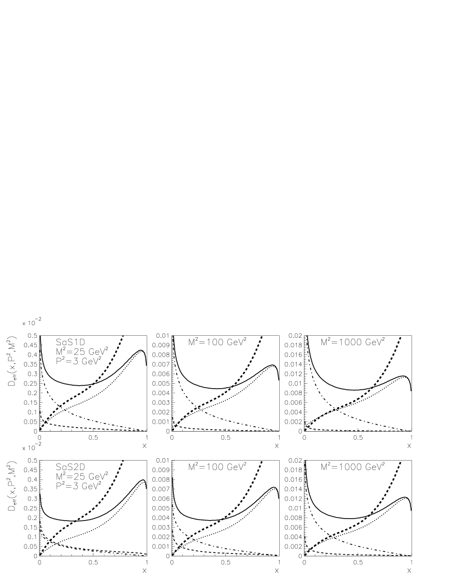
Figure 11: $D_{\mathrm{e}ff}(x,P^{2},M^{2})$ as a function of $x$ for $M^{2}=25,100,1000$ GeV² and $P^{2}=3$ GeV². Notation as in Fig. 6. In the splitting term $M_{0}^{2}=P^{2}$.

In realistic QCD the nonperturbative effects connected with the confinement, rather than current or constituent quark masses, are expected to determine the long–range structure of the photon and hence also the transition from the virtual photon to the real one. For instance, within the SaS parameterizations the role of quark masses is taken over by vector meson masses for the VDM components and by the initial $M_{0}$ for the pointlike ones. As in the case of the real photon, we recall basic features of SaS parameterizations of the virtual photon, illustrated in Figs. 7–10.

• With increasing $P^{2}$ the relative importance of VDM parts of both quark and gluon distribution functions with respect to the corresponding pointlike ones decreases rapidly. For $M^{2}\gtrsim 25$ GeV² the VDM parts of both SaS1D and SaS2D parameterizations become negligible for $P^{2}\gtrsim 2$ GeV², except in the region of very small $x\lesssim 0.01$. Consequently, also the ambiguity in the separation (17) is practically negligible in this region.

• The general pattern of scaling violations, illustrated in Fig. 8, remains the same as for the real photon, but there is a subtle difference, best visible when comparing in Fig. 4 the rescaled PDF for $P^{2}=0$ with those at $P^{2}=1,3$ GeV². While for $P^{2}=0$, increasing $M^{2}$ softens the spectrum towards the asymptotic pointlike form (22), for $P^{2}\gtrsim 1$ GeV² quark distribution functions increase with $M$ for practically all values of $x$. Moreover, while for $P^{2}=0$ the splitting term intersects the SaS1D curves qualitatively as in Fig. 2, for $P^{2}\gtrsim 1$ GeV² it is above them for all $x$ . These properties reflect the fact that SaS parameterizations of PDF of the virtual photon do not satisfy the same evolution equations as PDF of the real one. This difference is formally of power correction type and thus legitimate within the leading twist approximation we are working in, but numerically nonnegligible.

• As shown in Fig. 9 both VDM and pointlike parts decrease with increasing $P^{2}$, but the VDM parts drop much faster than the pointlike ones.

The implications of these properties for physical quantities $F_{2}^{\gamma}(x,P^{2},Q^{2})$ and $D_{\mathrm{e}ff}(x,P^{2},M^{2})$ are illustrated by Figs. 11 and 10. For $F_{2}^{\gamma}(x,P^{2},M^{2})$ the nontrivial aspects of virtual photon structure are confined mainly to the region of large $x$, where they reduce the predictions based on the splitting term (23). Obviously, only the pointlike quarks are relevant for this effect. The effects on $D_{\mathrm{e}ff}(x,P^{2},M^{2})$ worth emphasizing are the following:

• For all scales $M$ the contribution of the splitting term is above the one from pointlike quarks, the gap increasing with increasing $P^{2}$ and decreasing $M^{2}$.

• Pointlike quarks dominate $D_{\mathrm{e}ff}(x,P^{2},M^{2})$ at large $x$, whereas for $x\lesssim 0.3$, most of the pointlike contribution comes from the pointlike gluons. In particular, the excess of the pointlike contributions to $D_{\mathrm{e}ff}$ over the contribution of the splitting term, observed at $x\lesssim 0.5$, comes almost entirely from the pointlike gluons!

• For $x\gtrsim 0.6$ the full results are clearly below those given by the splitting term (23) with $M_{0}^{2}=P^{2}$. In this region one therefore expects the sum of subtracted direct and resolved contributions to jet cross–sections to be smaller than the results of unsubtracted direct calculations.

So far no restrictions were imposed on transverse energies and pseudorapidities of jets produced in $\gamma^{*}$p collisions. However, as discussed in more detail in Section 4.3.4, for jet transverse energies $E_{T}\gtrsim 5$ GeV, hadronization corrections become intolerably large and model dependent in the region $\eta\lesssim-2.5$. On the experimental side the problems with the reconstruction of jets with $E_{T}\gtrsim 5$ GeV in the forward region restrict the accessible region to $\eta\leq 0$. The cuts imposed on pseudorapidities $\eta^{(i)},i=1,2$ and transverse energies $E_{T}^{(i)}$ of two final state partons influence strongly the corresponding distribution in the variable $x_{\gamma}$

$$x_{\gamma}\equiv\frac{E_{T}^{(1)}e^{-\eta^{(1)}}+E_{T}^{(2)}e^{-\eta^{(2)}}}{2E_{\gamma}}$$ (45)

used in analyses of dijet data. At the LO and for massless partons $x_{\gamma}$ defined in (45) coincides with the conventional fraction $x$ appearing as an argument of photonic PDF. MC simulations show that for $E_{T}^{(i)}\geq 5~{}{\mathrm{GeV}}$ and $-2.5\leq\eta^{(i)}\leq 0,i=1,2$, $\langle x_{\gamma}\rangle\simeq 0.25$, is just the region where pointlike gluons dominate $D_{\mathrm{eff}}(x,P^{2},M^{2})$. This makes jet production in the region $P^{2}\gtrsim 1$ a promising place for identification of nontrivial aspects of PDF of virtual photons.

4 PDF of the virtual photon in NLO QCD calculations

Most of the existing information on interactions on virtual photons comes from the measurements of $F_{2}^{\gamma}$ at PETRA [18] and LEP [19] and jet production in ep collisions at HERA [20, 21]. In [21] data on dijet production in the region of virtualities $1\leq P^{2}\leq 80$ GeV², and for jet transverse energies $E_{T}^{\mathrm{j}et}\geq 5$ GeV have been analyzed within the framework of effective PDF defined in (25). This analysis shows that in the kinematical range $1~{}{\mathrm{GeV}}^{2}\lesssim P^{2}\ll E_{T}^{2}$ the data agree reasonably with the expectations based on SaS parameterizations of PDF of the virtual photon. The same data may, however, be also analyzed using the NLO parton level Monte–Carlo programs that do not introduce the concept of PDF of the virtual photon. Nevertheless, so long as $P^{2}\ll M^{2}\approx E_{T}^{2}$, the pointlike parts of PDF incorporate numerically important effects of a part of higher order corrections, namely those coming from collinear emission of partons in Fig. 1. This makes the concept of PDF very useful phenomenologically even for the virtual photon. To illustrate this point we shall now discuss dijet cross–sections calculated by means of JETVIP [25], currently the only NLO parton level MC program that includes both the direct and resolved photon contributions and which can thus be used to investigate the importance of the latter.

4.1 Structure of JETVIP

All the above mentioned parton level NLO MC programs contain the same full set of partonic cross–sections for the direct photon contribution up the order $\alpha\alpha_{s}^{2}$. Examples of such diagrams are in Fig. 12a ($\sigma(\alpha\alpha_{s})$ tree diagram) and Fig. 12b ($\sigma(\alpha\alpha_{s}^{2})$ tree diagram). Moreover all these programs contain also one–loop corrections to $\sigma(\alpha\alpha_{s})$ tree diagrams. They differ mainly in the technique used to regularize mass singularities: MEPJET and JETVIP employ the slicing method whereas DISENT and DISASTER use the subtraction method. Numerical comparison of JETVIP and the other codes can be found in [26, 27]. To go one order of $\alpha_{s}$ higher and perform complete calculation of the direct photon contributions up to order $\alpha\alpha_{s}^{3}$ would require evaluating tree diagrams like those in Fig. 12f,k, as well as one–loop corrections to diagrams like in Fig. 12b and two–loop corrections to diagrams like in Fig. 12a. So far, such calculations are not available.

In addition to complete NLO direct photon contribution JETVIP includes also the resolved photon one. Once the concept of virtual photon structure is introduced, part of the direct photon contribution, namely the splitting term (23), and in higher orders also further terms in (18), is subtracted from the direct contribution (which for the virtual photon is nonsingular) and included in PDF appearing in the resolved photon contribution. To avoid confusion we shall henceforth use the term “direct unsubtracted” (DIR_uns) to denote NLO direct photon contributions before this subtraction and reserve the term “direct” for the results after it. In this terminology the complete calculations is then given by the sum of direct and resolved parts and denoted DIR$+$RES.

At the order $\alpha_{s}^{2}$ the addition of resolved photon contribution means including diagrams like those in Fig. 12c-e, which involve convolutions of PDF from both proton and photon sides with $\sigma(\alpha_{s}^{2})$ tree partonic cross–sections. For a complete $O(\alpha_{s}^{2})$ calculation this is all that has to be added to the $O(\alpha\alpha_{s}^{2})$ partonic cross–sections in direct photon channel. However, for reasons discussed in detail in the next subsection, JETVIP includes also NLO resolved contributions, which involve convolutions of PDF with complete $\sigma(\alpha_{s}^{3})$ partonic cross–sections (examples of relevant diagrams are in Figs. 12g–j). This might seem inconsistent as no corresponding $\sigma(\alpha\alpha_{s}^{3})$ direct photon terms are included. Nevertheless, this procedure makes sense precisely because of a clear physical meaning of PDF of the virtual photon! Numerically, the inclusion of the $\sigma(\alpha_{s}^{3})$ resolved terms turns out to be very important and in certain parts of the phase space leads to large increase of JETVIP results compared to those of DISENT, MEPJET or DISASTER.

4.2 Factorization mechanism in $\gamma$p interactions

The main argument for adding $\sigma(\alpha_{s}^{3})$ partonic cross–sections in the resolved channel to $O(\alpha\alpha_{s}^{2})$ ones in the direct and $O(\alpha_{s}^{2})$ ones in the resolved channels, is based on specific way factorization mechanism works for processes involving photons in the initial state.

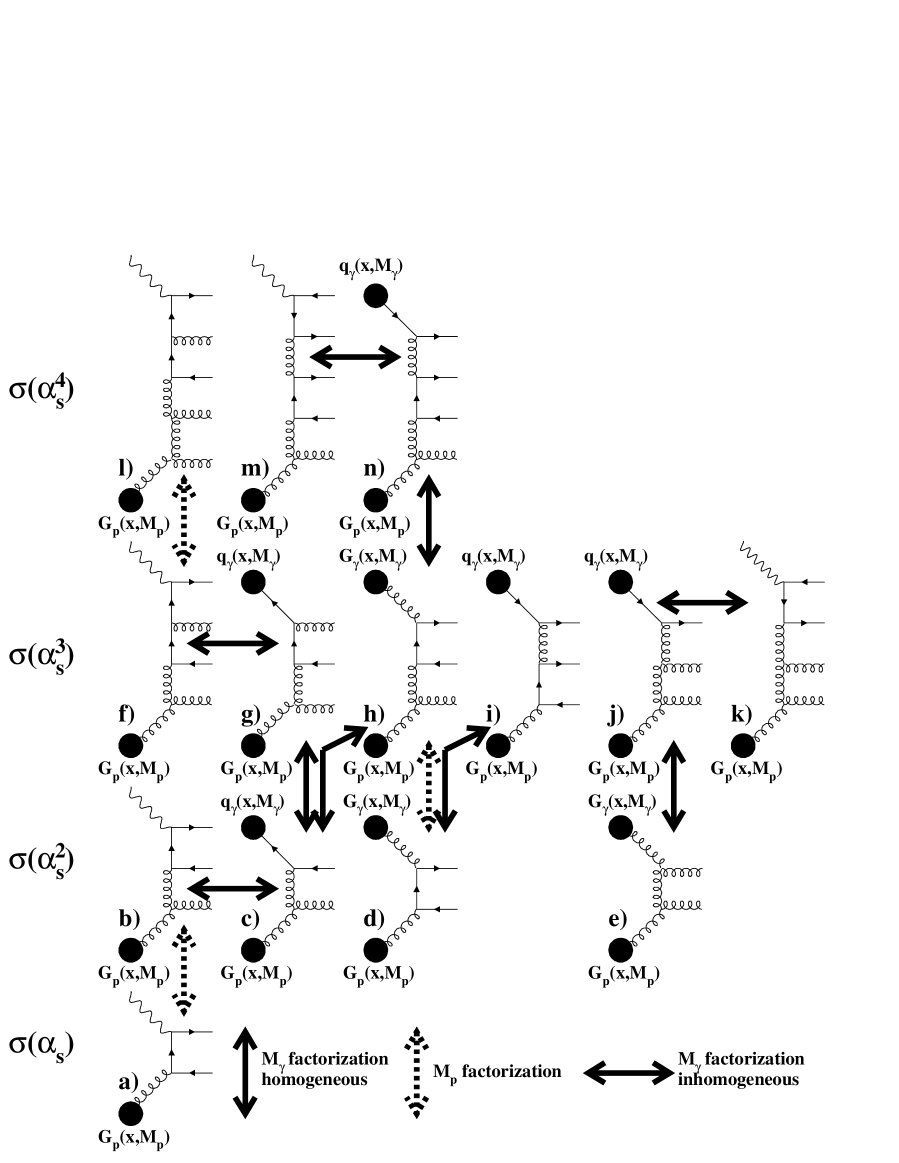
Figure 12: Examples of diagrams related by factorization mechanism. Only powers of $\alpha_{s}$ in parton level cross–sections are counted.

First, however, let us recall how the factorization works in hadronic collisions. Jet cross–sections start as convolutions of $\sigma(\alpha_{s}^{2})$ partonic cross–sections with PDF of beam and target hadrons. The factorization scale dependence of these PDF is cancelled by explicit factorization scale dependence of higher order partonic cross–sections. This cancellation is exact provided all orders of perturbation theory are taken into account, but only partial in any finite order approximation, like the NLO one used in analyses of jet production at FERMILAB. In hadronic collisions the inclusion of $\sigma(\alpha_{s}^{3})$ partonic cross–sections is thus vital for compensation of the factorization scale dependence of PDF in convolutions with $\sigma(\alpha_{s}^{2})$ partonic cross–sections. The residual factorization scale dependence of such NLO approximations is formally of the order $\alpha_{s}^{4}$ and thus one order of $\alpha_{s}$ higher than the terms included in the NLO approximation.

In $\gamma$p collisions (whether of real or virtual photon) the situation is different due to the presence of inhomogeneous terms $k_{q},k_{G}$ in the evolution equations (3–5). For quark distribution functions (nonsinglet as well as singlet) the leading term $(\alpha/2\pi)k_{q}^{(0)}$ in the expansion of $k_{q}$ is independent of $\alpha_{s}$ and consequently part of the factorization scale dependence of the $\sigma(\alpha_{s}^{2})$ resolved photon contribution is compensated at the same order $\alpha_{s}^{2}$. In further discussions we shall distinguish two factorization scales: one ($M_{\gamma}$) for the photon, and the other ($M_{p}$) for the proton. The content of the evolution equations (3–5) is represented graphically in Fig. 12, which shows examples of diagrams, up to order $\alpha_{s}^{4}$, relevant for our discussion. Some of these diagrams are connected by solid or dashed arrows, representing graphically the effects of variation of factorization scales $M_{\gamma}$ and $M_{p}$ respectively. The vertical dashed arrows connect diagrams (with lower blobs representing PDF of the proton, denoted $D_{p}(x,M_{p})$) that differ in partonic cross–sections by one order of $\alpha_{s}$, reflecting the fact that the terms on the r.h.s. of evolution equation for $D_{p}(x,M_{p})$ start at the order $\alpha_{s}$. For instance, the $\sigma(\alpha\alpha_{s})$ direct photon diagram in Fig. 12a is related by what we call $M_{p}$–factorization with $\sigma(\alpha\alpha_{s}^{2})$ direct photon diagram in Fig. 12b. Similarly, the $\sigma(\alpha_{s}^{2})$ resolved photon diagram in Fig. 12d is related by $M_{p}$–factorization to $\sigma(\alpha_{s}^{3})$ resolved photon diagram in Fig. 12h. In fact each diagram of the order $\alpha_{s}^{k}$ is related by $M_{p}$–factorization to two types of diagrams at order $\alpha_{s}^{k+1}$, one with quark and the other with gluon coming from the proton blob. Note that $M_{p}$–factorization operates within either direct or resolved contributions separately, never relating one type of terms with the other.

For $M_{\gamma}$–factorization this cancellation mechanism has a new feature. Similarly as for hadrons, the $\sigma(\alpha_{s}^{2})$ resolved photon diagram in Fig. 12c is related by what we call homogeneous $M_{\gamma}$–factorization to the $\sigma(\alpha_{s}^{3})$ resolved photon diagrams in Fig. 12g,h, and similar relation holds also between the diagram in Figs. 12e and 12j. However, the inhomogeneous term in evolution equation for PDF of the photon implies additional relation (which we call inhomogeneous $M_{\gamma}$–factorization) between direct and resolved photon diagrams at the same order of $\alpha_{s}$, represented by horizontal solid arrows. For instance, the LO resolved contribution coming from diagram in Fig. 12c is related not only by homogeneous $M_{\gamma}$–factorization to the $\sigma(\alpha_{s}^{3})$ resolved photon diagrams 12g-h, but also by inhomogeneous $M_{\gamma}$–factorization to the $\sigma(\alpha\alpha_{s}^{2})$ direct photon diagram in Fig. 12b. Similarly, the $\sigma(\alpha_{s}^{3})$ resolved photon diagram 12g is related by homogeneous $M_{\gamma}$–factorization to $\sigma(\alpha_{s}^{4})$ resolved terms (not shown) and by inhomogeneous $M_{\gamma}$–factorization to the $\sigma(\alpha\alpha_{s}^{3})$ direct diagram in Fig. 12f.

The argument for adding the $\sigma(\alpha_{s}^{3})$ resolved photon diagrams to the $\sigma(\alpha_{s}^{2})$ resolved photon ones relies on the fact that within the resulting set of NLO resolved contributions the homogeneous $M_{\gamma}$–factorization operates in the same way as the $M_{p}$–factorization does within the set of NLO direct ones! However, contrary to the hadronic case, the $\sigma(\alpha_{s}^{3})$ parton level cross–sections do not constitute after convolutions with photonic PDF a complete set of $\alpha\alpha_{s}^{3}$ contributions, the rest coming from the $\sigma(\alpha\alpha_{s}^{3})$ direct ones. As these $\sigma(\alpha\alpha_{s}^{3})$ direct photon contributions have not yet been calculated, the set of contributions included in JETVIP does not constitute the complete $O(\alpha\alpha_{s}^{3})$ calculation. The lacking terms, like that coming from the diagram 12f, would provide cancellation mechanism at the order $\alpha\alpha_{s}^{3}$ with respect to the inhomogeneous $M_{\gamma}$–factorization. In the absence of $\sigma(\alpha\alpha_{s}^{3})$ direct photon calculations, we thus have two options:

• To stay within the framework of complete $O(\alpha_{s}^{2})$ calculations, including the LO resolved and NLO direct contributions, but with no mechanism for the cancellation of the dependence of PDF of the virtual photon on the factorization scale $M_{\gamma}$.

• To add to the previous framework the $\sigma(\alpha_{s}^{3})$ resolved photon contribution, which provide the necessary cancellation mechanism with respect to homogeneous $M_{\gamma}$–factorization, but do not represent a complete set of $\sigma(\alpha_{s}^{3})$ contributions.

In our view the second strategy, adopted in JETVIP, is more appropriate. In fact one can look at $\sigma(\alpha_{s}^{3})$ resolved photon terms as results of approximate evaluation of the so far uncalculated $\sigma(\alpha\alpha_{s}^{3})$ direct photon diagrams in the collinear kinematics. For instance, so long as $P^{2}\ll M_{\gamma}^{2}$ taking into account only the pointlike part of $D_{\gamma}(x,P^{2},M_{\gamma}^{2})$ in the upper blob of Fig. 12g should be a good approximation of the contribution of the direct photon diagram in Fig. 12f. There are of course $\sigma(\alpha\alpha_{s}^{3})$ direct photon diagrams that cannot be approximated in this way, but we are convinced that it makes sense to build phenomenology on this framework.

For the $\sigma(\alpha_{s}^{2})$ resolved terms the so far unknown $\sigma(\alpha\alpha_{s}^{3})$ direct photon contributions provide the first chance to generate pointlike gluons inside the photon: the gluon in the upper blob in resolved photon diagram in Fig. 12e must be radiated by a quark that comes from primary $\gamma\rightarrow q\overline{q}$ splitting, for instance as shown in Fig. 12j. Note that to get the gluon in $\sigma(\alpha_{s}^{3})$ resolved photon contributions, for instance in Fig. 12h, within collinear limit of direct photon contributions would require evaluating diagrams, like that in Fig. 12m, at the order $\sigma(\alpha\alpha_{s}^{4})$! In summary, although the pointlike parts of quark and gluon distribution functions of the virtual photon are in a sense included in higher order perturbative corrections and can therefore be considered as expressions of “interactions” rather than “structure” of the virtual photon, their uniqueness and phenomenological usefulness definitely warrant their introduction as well as name.

4.3 Theoretical uncertainties

NLO calculations of jet cross–sections are affected by a number of ambiguities caused by the truncation of perturbation expansions as well as by uncertainties related to the input quantities and conversion of parton level quantities to hadron level observables.

4.3.1 Choice of PDF

We have taken CTEQ4M and SAS1D sets of PDF of the proton and photon respectively as our principal choice. Both of these sets treat quarks, including the heavy ones, as massless above their respective mass thresholds, as required by JETVIP, which uses LO and NLO matrix elements of massless partons. PDF of the proton are fairly well determined from global analyses of CTEQ and MRS groups and we have therefore estimated the residual uncertainty related to the choice of PDF of the proton by comparing the CTEQ4M results to those obtained with MRS(2R) set. The differences are very small, between 1% at $\eta=-2.5$ and 3.5% at $\eta=0$, independently of $P^{2}$.

For the photon we took the Schuler-Sjöstrand parameterizations for two reasons. First, they provide separate parameterizations of VDM and pointlike components of all PDF, which is crucial for physically transparent interpretation of JETVIP results. Secondly, they represent the only set of photonic PDF with physically well motivated virtuality dependence, which is compatible with the way JETVIP treats heavy quarks. The GRS sets [14, 15], the only other parameterizations with built-in virtuality dependence, are incompatible with JETVIP because they treat $c$ and $b$ quarks as massive and, consequently, require calculating their contribution to physical quantities via the boson gluon or gluon gluon fusion involving exact massive matrix elements.

4.3.2 The choice of $n_{f}$

JETVIP, as well as other NLO parton calculations of jet cross–sections, works with a fixed number $n_{f}$ of massless quarks, that must be chosen accordingly. This is not a simple task, as the number of quarks that can be considered effectively massless depends on kinematical variables characterizing the hardness of the collision. Consequently, the optimal choice of $n_{f}$ may not be unique for the whole kinematical region under consideration. The usual procedure is to run such programs for two (or more) relevant values of $n_{f}$ and use the ensuing difference as an estimate of theoretical uncertainty related to the approximate treatment of heavy quark contributions.

The number $n_{f}$ enters NLO calculations in three places: implicitly in $\alpha_{s}(\mu)$ and PDF and explicitly in LO and NLO parton level cross–sections. In our selected region of phase space the appropriate value of $n_{f}$ lies somewhere between $n_{f}=4$ and $n_{f}=5$, with the latter value representing the upper bound on the results (so far unavailable) that would take the $b$-quark mass effects properly into account. We have therefore run JETVIP for both $n_{f}=4$ and $n_{f}=5$ and compared their results. They differ, not suprisingly, very little . Explicit calculations give at most $10$% in the direct channel and $5$% in the resolve done. All the results presented below correspond to $n_{f}=5$.

4.3.3 Factorization and renormalization scale dependence

As mentioned in the previous subsection, proton and photon are associated in principle with different factorization scales $M_{p}$ and $M_{\gamma}$, but we followed the standard practice of assuming $M\equiv M_{p}=M_{\gamma}$ and set $M=\kappa E_{T}^{(1)}$. The factorization scale dependence was quantified by performing the calculations for $\kappa=0.5,1$ and $\kappa=2$.

The dependence of finite order perturbative calculations on the renormalization scale $\mu$ is in principle a separate ambiguity, but we have again followed the common practice of identifying these two scales $\mu=M$. To reflect this identification, we shall in the following use the term “scale dependence” to describe the dependence on this common scale.

4.3.4 Hadronization corrections

JETVIP, as a well as other NLO codes evaluate jet cross–sections at the parton level. For a meaningful comparison with experimental data they must therefore be corrected for effects describing the conversion of partons to observable hadrons. These so called hadronization corrections are not simple to define, but adopting the definition used by experimentalists [28] we have found that they depended sensitively and in a correlated manner on transverse energies and pseudorapidities of jets. In order to avoid regions of phase space where they become large we imposed on both jets the condition $-2.5\leq\eta^{(i)}\leq 0$. In this region hadronization corrections are flat in $\eta$ and do not exceed $10$%, whereas for $\eta\doteq-2.5$ they steeply rise with decreasing $\eta$. This by itself would not require excluding this region, the problem is that in this region hadronization corrections become also very much model dependent and therefore impossible to estimate reliably. Detailed analysis of various aspects of estimating these hadronization , with particular emphasize on their implication for jet production at HERA, is contained in [29].

4.3.5 Limitations of JETVIP calculations

Despite its undisputable advantage over the calculations that do not introduce the concept of virtual photon structure, also JETVIP has a drawback because it does not represent a complete NLO QCD calculation of jets cross–sections. This is true in the conventional approach to photonic interactions, and even more in the reformulation suggested by one of us in [1]. In the conventional approach the incompletness is related to the fact that there is no NLO parameterization of PDF of the virtual photon compatible with JETVIP treatment of heavy quarks. Note that in the standard approach the inclusion of $\sigma(\alpha_{s}^{3})$ partonic cross–sections in the resolved photon channel is justified by the claim that their convolution with photonic PDF are of the same order $\alpha\alpha_{s}^{2}$ as the direct photon ones. In the reformulation [1] this incompletness has deeper causes. It reflects the lack of appropriate input PDF but also the fact that a complete NLO approximation requires the inclusion of direct photon contribution of the order $\alpha\alpha_{s}^{3}$, which is so far not available. Nevertheless, we reiterate that it makes sense to build phenomenology upon the current JETVIP framework and the concept of PDF of the virtual photon is just the necessary tool for accomplishing it.

4.4 Dijet production at HERA

We shall now discuss the main features of dijet cross–sections calculated by means of JETVIP. To make our conclusions potentially relevant for ongoing analyses of HERA data we have chosen the following kinematical region

$$E_{T}^{(1)}\geq E_{T}^{c}+\Delta,~{}E_{T}^{(2)}\geq E_{T}^{c},~{}~{}~{}E_{T}^{c}=5~{}{\mathrm{GeV}},~{}~{}\Delta=2~{}{\mathrm{GeV}}$$

$$-2.5\leq\eta^{(i)}\leq 0,~{}i=1,2$$

in four windows of photon virtuality

$$1.4\leq P^{2}\leq 2.4~{}{\mathrm{GeV}}^{2};~{}2.4\leq P^{2}\leq 4.4~{}{\mathrm{GeV}}^{2};~{}4.4\leq P^{2}\leq 10~{}{\mathrm{G}eV}^{2};~{}10\leq P^{2}\leq 25~{}{\mathrm{GeV}}^{2}$$

The cuts on $E_{T}$ were chosen in such a way that throughout the region $P^{2}\ll E^{2}_{T}$, thereby ensuring that the virtual photon lives long enough for its “structure” to develop before the hard scattering takes place. The asymmetric cut option is appropriate for our decision to plot the sums of $E_{T}$ and $\eta$ distributions of the jets with highest and second highest $E_{T}$. The choice of $\Delta=2$ GeV, based on a detailed investigation [29] of the dependence of the integral over the selected region on $\Delta$, avoids the region where this dependence possesses unphysical features.

In our analysis jets are defined by means of the cone algorithm. At NLO parton level all jet algorithms are essentially equivalent to the cone one, supplemented with the parameter $R_{\mathrm{s}ep}$, introduced in [30] in order to bridge the gap between the application of the cone algorithm to NLO parton level calculations and to hadronic systems (from data or MC), where one encounters ambiguities related to seed selection and jet merging. In a general cone algorithm two objects (partons, hadrons or calorimetric cells) belong to a jet if they are within the distance $R$ from the jet center. Their relative distance satisfies, however, a weaker condition

$$\Delta R_{ij}=\sqrt{(\Delta\eta_{ij})^{2}+(\Delta\phi_{ij})^{2}}\leq\frac{E_{T_{i}}+E_{T_{j}}}{{\mathrm{m}ax}(E_{T_{i}},E_{T_{j}})}R.$$ (46)

The parameter $R_{\mathrm{s}ep}$ governs the maximal distance between two partons within a single jet, i.e. two partons form a jet only if their relative distance $\Delta R_{ij}$ satisfies the condition

$$\Delta R_{ij}\leq{\mathrm{m}in}\left[\frac{E_{T_{i}}+E_{T_{j}}}{{\mathrm{m}ax}(E_{T_{i}},E_{T_{j}})}R,R_{\mathrm{s}ep}\right].$$ (47)

The question which value of $R_{\mathrm{s}ep}$ to choose for the comparison of NLO parton level calculations with the results of the cone algorithm at the hadron level is nontrivial and we shall therefore present NLO results for both extreme choices $R_{\mathrm{s}ep}=R$ and $R_{\mathrm{sep}}=2R$. To define momenta of jets JETVIP uses the standard $E_{T}$–weighting recombination procedure, which leads to massless jets.

4.5 Results

To asses phenomenological importance of the concept of PDF of virtual photons we now compare JETVIP results obtained in the DIR_uns mode, where this concept is not introduced at all, with those of the DIR$+$RES one, in which the contribution of the resolved photon is added to the subtracted direct one. The difference between these two results measures the nontrivial aspects of PDF of the virtual photon.

Figure 13: Scale dependence of the distributions ${\mathrm{d}}\sigma/{\mathrm{d}}\eta$ and ${\mathrm{d}}\sigma/{\mathrm{d}}E_{T}$ at the NLO. All curves correspond to $R_{\mathrm{sep}}=2R$.

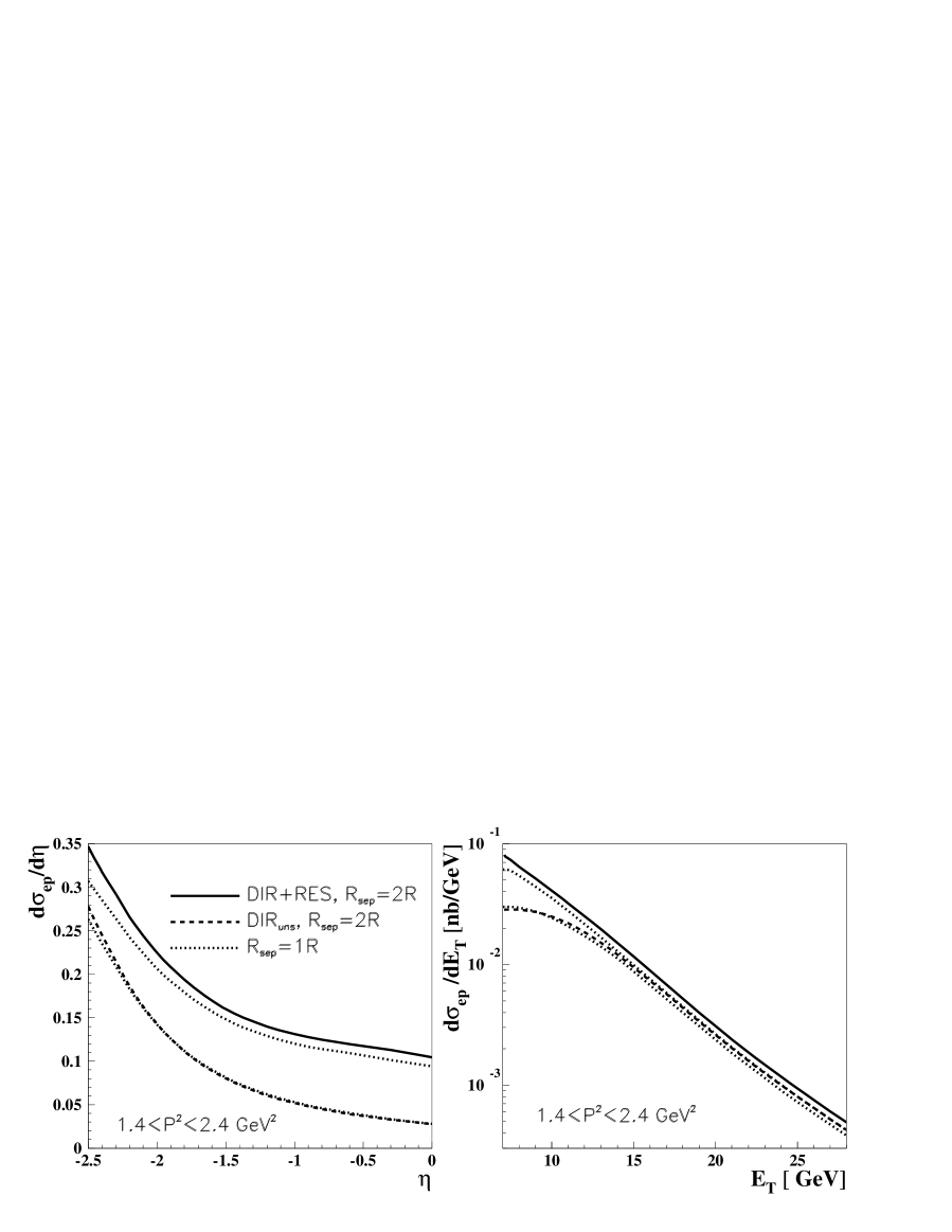
Figure 14: $R_{\mathrm{s}ep}$ dependence of ${\mathrm{d}}\sigma/{\mathrm{d}}\eta$ and ${\mathrm{d}}\sigma/{\mathrm{d}}E_{T}$ distributions. All curves correspond to $\mu=E_{T}$.

Figure 15: Comparison of DIR$+$RES, DIR_uns and DIR results for ${\mathrm{d}}\sigma/{\mathrm{d}}\eta$ (left plots) and individual contributions to ${\mathrm{d}}\sigma^{\mathrm{res}}/{\mathrm{d}}\eta$, described in the text (right plots). The thin solid curve corresponds to convolution of the splitting term (23) with $\sigma^{\mathrm{res}}_{q}(\alpha_{s}^{2})$ parton level cross–sections.

Figure 16: Fractional contributions to $\mathrm{d}\sigma^{\mathrm{res}}/\mathrm{d}\eta$. Upper and lower dotted (dashed–dotted) curves correspond to pointlike quarks (gluons) convoluted with $O(\alpha_{s}^{3})$ and $O(\alpha_{s}^{2})$ partonic cross–sections. The dashed curve in a) corresponds to the NLO VDM contribution. The solid curves denote the ratio DIR${}_{\mathrm{uns}}/$DIR$+$RES.

Figure 17: Nontriviality fractions $R_{3}$ and $R_{4}$ as functions of $\eta$ and $P^{2}$.

We start by plotting in Fig. 13 the distributions ${\mathrm{d}}\sigma/{\mathrm{d}}\eta$ and ${\mathrm{d}}\sigma/{\mathrm{d}}E_{T}$ in the first window $1.4\leq P^{2}\leq 2.4$ GeV². All curves correspond to $R_{\mathrm{s}ep}=2$. The difference between the solid and dashed curves is significant in the whole range of $\eta$, but becomes truly large close to the upper edge $\eta=0$, where the DIR$+$RES results exceed the DIR_uns ones by a factor of about 3! In ${\mathrm{d}}\sigma/{\mathrm{d}}E_{T}$ distributions this difference comes predominantly from the region of $E_{T}$ close to the lower cut–off $E_{T}^{c}+\Delta=7$ GeV. Fig. 13 also shows that the scale dependence is nonnegligible for both DIR_uns and DIR$+$RES results, but does not invalidate the main conclusion drawn from this comparison. Interestingly, the scale dependence is weaker for the DIR$+$RES results than for the DIR_uns ones. Fig. 14 documents that the above results depend only very weakly on $R_{\mathrm{s}ep}$.

To track down the origins of the observed large differences between DIR$+$RES and DIR_uns results we compare in Fig. 15 the DIR$+$RES and DIR_uns results to the subtracted direct ones (denoted DIR). The difference between the DIR$+$RES and DIR curves, giving the resolved photon contribution ${\mathrm{d}}\sigma^{\mathrm{r}es}/{\mathrm{d}}\eta$, is further split into the following contributions:

• VDM part of photonic PDF convoluted with complete NLO parton level cross–sections (denoted NLO VDM).

• Pointlike quarks and gluons convoluted with $\sigma^{\mathrm{res}}(\alpha_{s}^{2})$ and $\sigma^{\mathrm{res}}(\alpha_{s}^{3})$ parton level cross–sections

displayed separately in the upper right plot of Fig. 15. The full NLO resolved photon contribution is given as the sum

$$\mathrm{NLO~{}VDM}+\sigma_{q}^{\mathrm{res}}(\alpha_{s}^{2})\otimes q^{\mathrm{PL}}+\sigma_{G}^{\mathrm{res}}(\alpha_{s}^{2})\otimes G^{\mathrm{PL}}+\sigma_{q}^{\mathrm{res}}(\alpha_{s}^{3})\otimes q^{\mathrm{PL}}+\sigma_{G}^{\mathrm{res}}(\alpha_{s}^{3})\otimes G^{\mathrm{PL}}.$$ (48)

Fractional contributions of LO and NLO terms to $\sigma^{\mathrm{res}}$ coming separately from pointlike quarks and gluons are plotted in Fig. 16a as functions of $\eta$. Several conclusions can be drawn from Figs. 15–16:

• The contribution of the VDM part of photonic PDF is very small and perceptible only close to $\eta=0$. Integrally it amounts to about 3%. Using SaS2D parameterizations would roughly double this number.

• The inclusion of $\sigma_{i}^{\mathrm{res}}(\alpha_{s}^{3})$ parton level cross–sections in the resolved photon channel is numerically very important throughout the range $-2.5\leq\eta\leq 0$. Interestingly, the $\sigma_{i}^{\mathrm{res}}(\alpha_{s}^{3})$ results are close, particularly for the pointlike quarks, to the $\sigma_{i}^{\mathrm{res}}(\alpha_{s}^{2})$ ones.

• At both $\alpha_{s}^{2}$ and $\alpha_{s}^{3}$ orders pointlike quarks dominate ${\mathrm{d}}\sigma^{\mathrm{r}es}/{\mathrm{d}}\eta$ at large negative $\eta$, whereas as $\eta\rightarrow 0$ the fraction of ${\mathrm{d}}\sigma^{\mathrm{r}es}/{\mathrm{d}}\eta$ coming from pointlike gluons increases towards $40$% at $\eta=0$.

We emphasize that pointlike gluons carry nontrivial information already in convolutions with $\sigma^{\mathrm{res}}(\alpha_{s}^{2})$ partonic cross–sections because in unsubtracted direct calculations such contributions would appear first at the order $\alpha\alpha_{s}^{3}$ . The convolution of the dominant part of pointlike quarks with $\sigma^{\mathrm{res}}(\alpha_{s}^{3})$ partonic cross–sections would be included in direct unsubtracted calculations starting also at the order $\alpha\alpha_{s}^{3}$, whereas for pointlike gluons this would require evaluating the unsubtracted direct terms of even higher order $\alpha\alpha_{s}^{4}$! For instance, the contribution of diagram in Fig. 12g would be included in the contribution of diagram in Fig. 12f. Similarly, the results of diagram in Fig. 12h would come as part of the results of evaluating the diagram in Fig. 12m.

In JETVIP the nontrivial aspects of taking into account the $\sigma_{i}^{\mathrm{res}}(\alpha_{s}^{3})$ resolved photon contributions can be characterized by the “nontriviality fractions” $R_{3}$ and $R_{4}$

$$R_{3}\equiv\frac{q^{\mathrm{PL}}\otimes\sigma_{q}^{\mathrm{res}}(\alpha_{s}^{3})+G^{\mathrm{PL}}\otimes\sigma_{G}^{\mathrm{res}}(\alpha_{s}^{2})}{\sigma^{\mathrm{res}}},~{}~{}~{}R_{4}\equiv\frac{G^{\mathrm{PL}}\otimes\sigma_{G}^{\mathrm{res}}(\alpha_{s}^{3})}{\sigma^{\mathrm{res}}},$$ (49)

which quantify the fractions of $\sigma^{\mathrm{res}}$ that are not included in NLO unsubtracted direct calculations. These fractions are plotted as functions of $\eta$ and $P^{2}$ in Fig. 17. Note that at $\eta=0$ almost 70% of $\sigma^{\mathrm{res}}$ comes from these origins. This fraction rises even further in the region $\eta>0$, which, however, is experimentally difficult to access.

So far we have discussed the situation in the first window of photon virtuality, i.e. for $1.4\leq P^{2}\leq 2.4$ GeV². As $P^{2}$ increases the patterns of scale and $R_{\mathrm{sep}}$ dependencies change very little. On the other hand, the fractions plotted in Fig. 16 and 17 vary noticeably:

• The DIR_uns contributions represent an increasing fractions of the DIR$+$RES results.

• The relative contribution of pointlike gluons with respect to pointlike quarks decreases.

• The nontriviality factor $R_{4}$ (which comes entirely from pointlike gluons) decreases, whereas $R_{3}$, which is dominated by pointlike quarks and flat in $\eta$, is almost independent of $P^{2}$.

All these features of JETVIP results reflect the fundamental fact that as $P^{2}$ rises towards the factorizations scale $M^{2}\approx E_{T}^{2}$ the higher order effects incorporated in pointlike parts of photonic PDF vanish and consequently the unsubtracted direct results approach the DIR$+$RES ones. The crucial point is that for pointlike quarks and gluons this approach is governed by the ratio $P^{2}/M^{2}$ appearing in the multiplicative factor $(1-P^{2}/M^{2})$. The nontrivial effects included in PDF of the virtual photon will thus persist for arbitrarily large $P^{2}$, provided we stay in the region where $P^{2}\ll M^{2}$. Moreover, they are so large, that they should be visible already in existing HERA data. Provided the basic ideas behind the Schuler–Sjöstrand parameterizations of PDF of the virtual photon are correct, our analysis shows that the calculations that do not introduce the concept of virtual photon structure should significantly undershoot the available HERA data on dijet production in the kinematical region $1\lesssim P^{2}\ll E_{T}^{2},~{}E_{T}\geq 5$ GeV, $-2.5\leq\eta\leq 0$, in particular for $\eta\simeq 0$. Published as well preliminary data discussed in [29, 31] support this conjecture.

5 Summary and conclusions

We have analyzed the physical content of parton distribution functions of the virtual photon within the framework formulated by Schuler and Sjöstrand, which provides physically motivated separation of quark and gluon distribution functions into their hadronic (VDM) and pointlike parts. We have shown that the inherent ambiguity of this separation, numerically large for the real photon, becomes phenomenologically largely irrelevant for virtual photons with $P^{2}\gtrsim 2-3$ GeV². In this region quark and gluon distribution functions of the virtual photon are dominated by their (reasonably unique) pointlike parts, which have clear physical origins. We have analyzed the nontrivial aspects of these pointlike distribution functions and, in particular, pointed out the role of pointlike gluons in leading order calculations of jet cross–section at HERA.

The conclusions made within the framework of LO QCD have been confirmed, and in a sense even strengthened, in our analysis of NLO parton level calculations using JETVIP. We have found a significant difference between JETVIP results in approaches with and without the concept of virtual photon structure. While for the real photon analogous difference is in part ascribed to the VDM part of photonic PDF, for moderately virtual photons it comes almost entirely from the pointlike parts of quark and gluon distribution functions. Although their contributions are in principle contained in higher order calculations which do not use the concept of PDF, in practice this would require calculating at least $\sigma(\alpha\alpha_{s}^{3})$ and $\sigma(\alpha\alpha_{s}^{4})$ unsubtracted direct contributions. In the absence of such calculations the concept of PDF of the virtual photon is therefore very useful phenomenologically and, indeed, indispensable for satisfactory description of existing data.

Acknowledgment: We are grateful to J. Cvach, J. Field, Ch. Friberg, G. Kramer, B. Pötter, I. Schienbein and A. Valkárová for interesting discussions concerning the structure and interactions of virtual photons and to B. Pötter for help in running JETVIP. This work was supported in part by the Grant Agency of the Academy od Sciences of the Czech Republic under grant No. A1010821.

References

- [1] J. Chýla: hep-ph/9911413
- [2] W. Bardeen, A. Buras, D. Duke and T. Muta, Phys. Rev D18, 3998 (1978)
- [3] J. Chýla, Z. Phys. C43, 431 (1989)
- [4] G. Curci, W. Furmanski, R. Petronzio, Nucl. Phys. B175, 27 (1980)
-
[5]
P. Aurenche, R. Baier, A. Douiri, M. Fontannaz,
D. Schiff, Nucl. Phys. B286, 553 (1987)
P. Aurenche, R. Baier, M. Fontannaz, D. Schiff, Nucl. Phys. B296, 661 (1987) - [6] J. Chýla, M. Taševský, in Proceedings PHOTON ’99, Freiburg in Breisgau, May 1999, ed. S. Soeldner–Rembold, Nucl. Phys. Proc. Supp., in press, hep-ph/9906552
-
[7]
G. Schuler, T. Sjöstrand: Z. Phys. C68
(1995), 607
G. Schuler, T. Sjöstrand: Phys. Lett. B376 (1996),193 -
[8]
J.H. Field, F. Kapusta, L. Poggioli, Phys. Lett.
B181, 362 (1986)
J.H. Field, F. Kapusta, L. Poggioli, Z. Phys. C36, 121 (1987)
F. Kapusta, Z. Phys. C42, 225 (1989) - [9] E. Witten: Nucl. Phys. 120 (1977). 189
- [10] W. Bardeen, A. Buras, Phys. Rev. D20, 166 (1979)
- [11] J. Chýla: Phys. Lett. B320 (1994), 186
- [12] J. Chýla: hep–ph/9811455
- [13] A. Gorski, B.L. Ioffe, A. Yu. Khodjamirian, A. Oganesian, Z. Phys. C 44, 523 (1989)
-
[14]
M. Glück, E. Reya, M. Stratmann, Phys. Rev. D51
(1995), 3220
M. Glück, E. Reya, M. Stratmann, Phys. Rev. D54 (1996), 5515 - [15] M. Glück, E. Reya, I. Schienbein, Phys. Rev. D60 (1999), 054019
- [16] J. Chýla, M. Taševský, in preparation
- [17] J. Chýla, M. Taševský, in Proceedings of Workshop MC generators for HERA Physics, Hamburg 1999, p. 239, hep-ph/9905444
- [18] Ch. Berger et al. (PLUTO Collab.), Phys. Lett. B142 (1984), 119
- [19] F. Erné, in Proceedings PHOTON ’99, Freiburg in Breisgau, May 1999, ed. S. Soeldner–Rembold, Nucl. Phys. Proc. Supp., in press, L3 Note 2403, submitted to Europhysics Conference High Energy Physics, Tampere, August 1999
- [20] C. Adloff et al. (H1 Collab.), Phys. Lett. B415 (1997), 418
- [21] C. Adloff et al. (H1 Collab.), Eur. Phys. J. C, in press
- [22] S. Catani, M. Seymour, Nucl. Phys. B458 (1997), 291, Erratum-ibid. B510 (1997), 503
- [23] E. Mirkes, TTP-97-39, hep-ph/9711224
- [24] D. Graudenz, hep-ph/9710244
-
[25]
B. Pötter, Comp. Phys. Comm. 119 (1999),
45, hep–ph/9806437
G. Kramer, B. Pötter, Eur. Phys. J. C5 (1998), 665, hep–ph/9804352 - [26] C. Duprel, Th. Hadig, N. Knauer, M. Wobisch, in Proceedings of Workshop MC generators for HERA Physics, Hamburg 1999, p. 142, hep-ph/9910448
- [27] B. Pötter, hep-ph/9911221
- [28] M. Wobisch, in Proceedings of Workshop MC generators for HERA Physics, Hamburg 1999, p. 239, hep-ph/9905444
- [29] M. Taševský, PhD Thesis, unpublished
- [30] S.D.Ellis, Z. Kunszt, D.E. Soper, Phys. Rev. Lett. 69 (1992), 3615
- [31] J. Cvach, in Proceedings DIS99, Nucl. Phys. B (Proc. Suppl.) 79 (1999), 501