bla

Analysis of ${\cal O}(p^{2})$ Corrections to $\langle\pi\pi|{\cal Q}_{7,8}|K\rangle$

Vincenzo Cirigliano^a and Eugene Golowich^b

^a Dipartimento di Fisica dell’Università and I.N.F.N.

Via Buonarroti,2 56100 Pisa (Italy)

vincenzo@het2.physics.umass.edu

^b Department of Physics and Astronomy

University of Massachusetts

Amherst MA 01003 USA

gene@het2.physics.umass.edu

The one-loop corrections to $K\to\pi$ and $K\to 2\pi$ matrix elements of the electroweak penguin operator are calculated. General next-to-leading order relations between the $K\to\pi$ and $K\to 2\pi$ amplitudes are obtained. The fractional shift $\Delta_{2}=0.27\pm 0.27$ is found for the ${\cal O}(p^{2})$ corrections to a recent chiral determination of $\langle(\pi\pi)_{I=2}|{\cal Q}_{7,8}|K^{0}\rangle$. We explain why the sign for $\Delta_{2}$ is opposite to that expected from unitarization approaches based on the Omnès equation. We perform a background-field, heat-kernel determination of the divergent one-loop amplitudes for a general class of (V-A)$\times$(V+A) operators.

1 Introduction

In the Standard Model, $K\to\pi\pi$ amplitudes are conveniently expressed in terms of the effective nonleptonic $\Delta S=1$ hamiltonian,

$$\langle\pi\pi|{\cal H}_{\Delta S=1}|K\rangle={G_{F}\over\sqrt{2}}V_{ud}V_{us}^{*}\sum_{i=1}^{10}\ c_{i}(\mu)~{}\langle\pi\pi|{\cal Q}_{i}|K\rangle_{\mu}\ \ ,$$ (1)

where $\{{\cal Q}_{i}\}$ are local four-quark operators, $\{c_{i}(\mu)\}$ are constants, and $\mu$ is a renormalization scale. In order to determine the $K\to\pi\pi$ amplitudes, one must be able to calculate the matrix elements $\langle\pi\pi|{\cal Q}_{i}|K\rangle_{\mu}$. The study of such matrix elements has continued to be an active research area because of what it can teach us about the inner workings of low energy QCD. Interest has been recently heightened by the KTeV and NA48 announcements [1] that $\epsilon^{\prime}/\epsilon\simeq 20\cdot 10^{-4}$, to be compared to the approximate theoretical relation

$${\epsilon^{\prime}\over\epsilon}=10\times 10^{-4}\bigg{[}-3.1~{}{\rm GeV}^{-3}\cdot\langle(\pi\pi)_{I=0}|{\cal Q}_{6}|K^{0}\rangle$$

$$\phantom{xxxxxxx}-0.51~{}{\rm GeV}^{-3}\cdot\langle(\pi\pi)_{I=2}|{\cal Q}_{8}|K^{0}\rangle\bigg{]}\ \ ,$$ (2)

evaluated in the NDR scheme at scale $\mu=2$ GeV.

In the application of chiral symmetry to this problem, the $K\to\pi\pi$ matrix elements are expanded in powers of the external momenta and quark masses. It is especially attractive to consider matrix elements which do not vanish in the chiral limit, such as those of the electroweak penguin operators

$${\cal Q}_{7}\ =\ {3\over 2}\left({\bar{s}}_{i}~{}d_{i}\right)_{\rm V-A}\sum_{q=u,d,s}~{}Q_{q}\left({\bar{q}}_{j}~{}q_{j}\right)_{\rm V+A}\ \ ,$$

$${\cal Q}_{8}\ =\ {3\over 2}\left({\bar{s}}_{i}~{}d_{j}\right)_{\rm V-A}\sum_{q=u,d,s}~{}Q_{q}\left({\bar{q}}_{j}~{}q_{i}\right)_{\rm V+A}\ \ ,$$ (3)

where $Q_{q}$ is the electric charge of quark $q$ and $i,j$ are color labels. Working in the chiral limit, Donoghue and Golowich [2] recently evaluated the leading chiral component to $\langle(\pi\pi)_{I=2}|{\cal Q}_{8}|K^{0}\rangle$ and also $\langle(\pi\pi)_{I=2}|{\cal Q}_{7}|K^{0}\rangle$. In this paper, we use chiral perturbation theory (ChPT) to extend this by calculating the ${\cal O}(p^{2})$ chiral corrections to matrix elements of ${\cal Q}_{7}$ and ${\cal Q}_{8}$.

Given the flavor and chiral structure of ${\cal Q}_{7,8}$, there exists a unique operator at ${\cal O}(p^{0})$ that represents them in an effective chiral description,

$${\cal O}_{\rm ewp}=g\,\mbox{Tr}\,\left[\lambda_{6}UQU^{\dagger}\right]\ \ .$$ (4)

The operator ${\cal O}_{\rm ewp}$ in turn belongs to a family of chiral operators ${\cal O}_{ab}$ which transform as members of ${\bf 8}_{L}\times{\bf 8}_{R}$ under chiral rotations,

$${\cal O}_{ab}=\mbox{Tr}\,\left[\lambda_{a}U\lambda_{b}U^{\dagger}\right]\ \ .$$ (5)

In Eqs. (4),(5), $\lambda_{a}$ is a Gell Mann matrix, $Q=~{}diag~{}(2/3,-1/3,-1/3)$ is the quark charge matrix and $U$ is the matrix of light pseudoscalar fields,

$$U\equiv\exp(i\lambda_{k}\Phi_{k}/F)\ \ (k=1,\dots,8)\ \ ,$$ (6)

where $F$ is the pseudoscalar meson decay constant in lowest order. The coupling constant $g$ in Eq. (4) will depend on the ‘parent’ operator (${\cal Q}_{7,8}$ in our case) and can be obtained by comparison with an evaluation of the matrix elements performed in the chiral limit (analytically as in Ref. [2] or QCD lattice-theoretic as in Ref. [3]).

The standard first step in a ChPT analysis is to work in the chiral world of zero momentum and vanishing light quark mass. This leading chiral component, if nonzero, often provides the largest contribution to the matrix element. In the chiral limit, moreover, simple linear relations exist among amplitudes with differing numbers of Goldstone modes. In particular, knowledge of the $K\rightarrow\pi$ matrix elements is sufficient to extract the physical $K\rightarrow\pi\pi$ matrix elements.

Experience has shown, however, the necessity for calculating chiral corrections. This is especially true for amplitudes involving kaons, as the possibility of sizeable chiral corrections (of order $25\%$ or more) cannot be excluded when passing from $m_{K}=0$ to $m_{K}=0.495$ GeV. [4] This calls for an ${\cal O}(p^{2})$ analysis in the chiral representation of weak operators. At this order the chiral determination of $K\rightarrow n\pi$ matrix elements of ${\cal Q}_{7,8}$ includes two basic ingredients:

1. One-loop diagrams with insertion of vertices from ${\cal O}_{\rm ewp}$ (cf Eq. (4)). We calculate in dimensional regularization, using a scale parameter $\mu_{\chi}$.

2. Tree-level diagrams with insertion of the ${\cal O}(p^{2})$ counterterm operators (to be described in Sect. 2).

In the $K\to\pi$ sector, for example, the ${\cal O}(p^{2})$ amplitudes arise from the contributions depicted in Figure 1. In Fig. 1(a), a loop begins and ends at the electroweak vertex, whereas in Fig. 1(b) the electroweak vertex is an insertion in the loop which is produced by a strong interaction vertex.

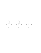
Figure 1: $K\to\pi$ contributions: (a) weak vertex, (b) strong and weak vertices, (c) counterterm.

An important component of our calculation will be a leading-log estimate of the ${\cal O}(p^{2})$ corrections (cf Eq. (41)). This provides only a partial estimate of the full ${\cal O}(p^{2})$ effect because it leaves out the contribution from the finite counterterms. Recall that divergences encountered in the loop diagrams are cancelled by divergences in the counterterm coefficents, leaving just the finite loop and counterterm amplitudes. Each of these is dependent on the scale $\mu_{\chi}$, but the total amplitude is scale-independent. Unfortunately, the finite counterterm coefficients are unknown at this time. Therefore we base our estimation of ${\cal O}(p^{2})$ corrections on the finite part of the loop amplitude and determine the accompanying uncertainty by numerically studying its dependence on $\mu_{\chi}$.

In practice, first-principle calculations tend to reliably handle only the relatively simple $K\rightarrow\pi$ matrix elements. It is not clear that this information is sufficient to recover matrix elements for multipion final states. Indeed, reconstruction of the physical $K\rightarrow\pi\pi$ matrix elements is known to be nontrivial at next-to-leading order. An advantage of the ChPT approach is that it provides independent calculations of the $K\to\pi$ and $K\to\pi\pi$ transitions. A significant aspect of our investigation will be to check whether the the ${\cal O}(p^{2})$ $K\rightarrow\pi$ matrix elements are sufficient to fully determine the the ${\cal O}(p^{2})$ $K\rightarrow\pi\pi$ matrix elements.

Our presentation is arranged as follows. In Section 2 we list the ${\cal O}(p^{2})$ chiral operators representing ${\cal Q}_{7,8}$ and then perform the one-loop renormalizaztion of the generating functional with insertions of the generic operator ${\cal O}_{ab}$ (see Eq. (5)). In Section 3 we present the ${\cal O}(p^{2})$ analysis for $\langle\pi|{\cal Q}_{7,8}|K\rangle$ and $\langle\pi\pi|{\cal Q}_{7,8}|K\rangle$, including loop and counterterm contributions. Then, in Section 4 we perform a first numerical evaluation (based on chiral loops only) of the corrections to the leading chiral component of $\langle\pi\pi|{\cal O}_{7,8}|K\rangle$. The main results of this work are summarized and future studies are outlined in Section 5. Finally, we note that throughout the paper $K\to n\pi$ matrix elements of a local operator ${\cal O}$ are expressed as

$${\cal M}_{K\to\pi}=\langle\pi(p_{\pi})|{\cal O}|K(p_{k})\rangle\quad{\rm and}\quad{\cal M}_{K\to\pi_{1}\pi_{2}}=\langle\pi(p_{1})\pi(p_{2})|{\cal O}|K(p_{k})\rangle\ \ .$$ (7)

2 Counterterm Lagrangians

In the following we first display the list of ${\cal O}(p^{2})$ counterterms which share the chiral properties of the ${\cal O}(p^{0})$ operator ${\cal O}_{\rm ewp}$. Presentation of the various $K\to\pi$ and $K\to\pi\pi$ counterterm matrix elements is deferred to later in the paper.

With each counterterm operator will be associated a coefficient which is a priori arbitrary. Some of these counterterm coefficients need to be singular in order to cancel divergences which appear in the one-loop amplitudes. In the second part of this section, we employ background field and heat kernel methods to determine the set of singular ${\cal O}(p^{2})$ coefficients.

2.1 The Set of Counterterm Lagrangians

There are seven effective operators at chiral order $p^{2}$ associated with the operator ${\cal O}_{ab}$ of Eq. (5),

$${\cal L}^{ab}_{\rm ct}=\sum_{k=1}^{7}\ c_{k}{\cal O}_{k}^{(ab)}\ \ ,$$ (8)

with

$${\cal O}_{1}^{(ab)} = \,{\rm Tr}\,\left[\lambda_{a}D_{\mu}U\lambda_{b}D^{\mu}U^{\dagger}\right]\ \ ,$$

$${\cal O}_{2}^{(ab)} = \,{\rm Tr}\,\left[\lambda_{a}UD_{\mu}U^{\dagger}\right]\cdot\,{\rm Tr}\,\left[\lambda_{b}U^{\dagger}D^{\mu}U\right]\ \ ,$$

$${\cal O}_{3}^{(ab)} = \,{\rm Tr}\,\left[\lambda_{a}U\lambda_{b}D_{\mu}U^{\dagger}D^{\mu}U~{}U^{\dagger}+\lambda_{a}UD_{\mu}U^{\dagger}D^{\mu}U~{}\lambda_{b}U^{\dagger}\right]\ \ ,$$

$${\cal O}_{4}^{(ab)} = \,{\rm Tr}\,\left[\lambda_{a}U\lambda_{b}SU^{\dagger}+\lambda_{a}US\lambda_{b}U^{\dagger}\right]\ \ ,$$

$${\cal O}_{5}^{(ab)} = i\,{\rm Tr}\,\left[\lambda_{a}U[P,\lambda_{b}]U^{\dagger}\right]\ \ ,$$

$${\cal O}_{6}^{(ab)} = \,{\rm Tr}\,\left[\lambda_{a}U\lambda_{b}U^{\dagger}\right]\cdot\,{\rm Tr}\,\left[\chi U^{\dagger}+\chi^{\dagger}U\right]\ \ ,$$

$${\cal O}_{7}^{(ab)} = \,{\rm Tr}\,\left[\lambda_{a}U\lambda_{b}U^{\dagger}\right]\cdot\,{\rm Tr}\,\left[D_{\mu}UD^{\mu}U^{\dagger}\right]\ \ ,$$ (9)

where the quantities $S$ and $P$ occurring respectively in ${\cal O}_{4}^{(ab)}$ and ${\cal O}_{5}^{(ab)}$ are defined as

$$S\equiv U^{\dagger}\chi+\chi^{\dagger}U\qquad{\rm and}\qquad P\equiv i\left(U^{\dagger}\chi-\chi^{\dagger}U\right)\ .$$ (10)

The possible two-derivative dependence $D_{\mu}D^{\mu}U$ has been eliminated by using the equations of motion,

$$D^{\mu}\left(U^{\dagger}D_{\mu}U\right)+{1\over 2}\left(\chi^{\dagger}U-U^{\dagger}\chi\right)=0\ \ .$$ (11)

The case of interest for this paper (involving the operator ${\cal O}_{\rm ewp}$ of Eq. (4)) is recovered with the replacements $\lambda_{a}\to\lambda_{6}$ and $\lambda_{b}\to Q$. Calculation of the set of counterterm amplitudes is straightforward and is summarized in Sect. 3.2.

2.2 Divergences in the One-loop Effective Action

The effective chiral lagrangian on which the one-loop analysis is based is

$${\cal L}\ =\ {\cal L}^{(2)}_{\rm str}+{\cal O}_{\rm ewp}\ \ ,$$ (12)

where ${\cal O}_{\rm ewp}$ is defined in Eq. (4) and ${\cal L}^{(2)}_{\rm str}$ is the familiar $\Delta S=0$ lagrangian,

$${\cal L}^{(2)}_{\rm str}={F^{2}_{0}\over 4}\,{\rm Tr}\,\left(D_{\mu}UD^{\mu}U^{\dagger}\right)+{F^{2}_{0}\over 4}\,{\rm Tr}\,\left(\chi U^{\dagger}+U\chi^{\dagger}\right)\ \ .$$ (13)

We shall calculate quantum corrections about a solution ${\overline{U}}$ of the classical theory. To accomplish this, we employ background field and heat kernel methods. Thus we write

$$U\ =\ {\overline{U}}~{}e^{i\Delta}\ \ ,$$ (14)

where $\Delta=\lambda^{a}\Delta^{a}$ represents the quantum fluctuations. We begin by expressing the generating functional at one-loop order as

$$e^{i{\cal Z}}=e^{i\int d^{4}x\left[{\cal L}({\overline{U}})+{\cal L}_{\rm ct}({\overline{U}})\right]}\cdot\int[dU]~{}e^{i\int d^{4}x~{}\left[{\cal L}(U)-{\cal L}({\overline{U}})\right]}\ \ ,$$ (15)

where ${\cal L}$ is given in Eq. (12) and ${\cal L}_{\rm ct}$ is the counterterm lagrangian of Eq. (8) with $\lambda_{a}\to\lambda_{6}$ and $\lambda_{b}\to Q$. Keeping just the part quadratic in $\Delta$, we have

$${\cal L}(U)-{\cal L}({\overline{U}})=-{F^{2}\over 2}\Delta_{a}\left(d_{\mu}d^{\mu}+\sigma+w\right)^{ab}\Delta_{b}+\dots\ \ ,$$ (16)

where

$$d_{\mu}^{ab}=\delta^{ab}\partial_{\mu}+\Gamma_{\mu}^{ab}\ ,$$

$$\Gamma_{\mu}^{ab}=-{1\over 4}\,{\rm Tr}\,\left[[\lambda^{a},\lambda^{b}]\left({\overline{U}}^{\dagger}\partial_{\mu}{\overline{U}}+i{\overline{U}}^{\dagger}\ell_{\mu}{\overline{U}}+ir_{\mu}\right)\right]\ ,$$

$$\sigma^{ab}={1\over 8}\,{\rm Tr}\,\bigg{[}[\lambda^{a},\lambda^{b}]_{+}\left(\chi U^{\dagger}+U\chi^{\dagger}\right)+[\lambda^{a},{\overline{U}}^{\dagger}\partial_{\mu}{\overline{U}}]~{}[\lambda^{a},{\overline{U}}^{\dagger}\partial^{\mu}{\overline{U}}]\bigg{]}\ ,$$

$$w^{ab}=-{g\over F^{2}}\,{\rm Tr}\,\bigg{[}\lambda_{6}{\overline{U}}\left(\lambda^{a}Q\lambda^{b}+\lambda^{b}Q\lambda^{a}-{1\over 2}[[\lambda^{a},\lambda^{b}]_{+},Q]_{+}\right){\overline{U}}^{\dagger}\bigg{]}\ \ .$$

(17)

In the above $\ell_{\mu}$ and $r_{\mu}$ are source functions coupled to chiral currents. The integrand occurring in Eq. (15) is gaussian and thus allows for direct evaluation of the path integral,

$${\cal Z}_{\rm 1-loop}=\int d^{4}x\ \left[{\cal L}({\overline{U}})+{\cal L}_{\rm ct}({\overline{U}})\right]+{i\over 2}\,{\rm tr}\,\log\left(d_{\mu}d^{\mu}+\sigma+w\right)\ \ ,$$ (18)

where ‘$tr$’ indicates a sum over spacetime coordinates as well as flavor labels.

By using the heat kernel expansion, we identify the divergences in ${\cal Z}_{\rm 1-loop}$ as

$${\cal Z}_{\rm 1-loop}^{\rm(div)}={1\over 2(4\pi)^{d/2}}\int d^{4}x\ \Gamma\left({\epsilon\over 2}\right)~{}\,{\rm Tr}\,\left[{1\over 12}\Gamma_{\mu\nu}\Gamma^{\mu\nu}+{1\over 2}\left(\sigma+w\right)^{2}\right]\ \ ,$$ (19)

where $\epsilon\equiv 4-d$ and $\Gamma_{\mu\nu}^{ab}=[d_{\mu},d_{\nu}]^{ab}$. There is a great deal of content in Eq. (19), including the one-loop divergent contributions to the Gasser-Leutwyler ${\cal O}(p^{4})$ strong lagrangian. [9, 10] However, we require only the new piece which arises from the interference between the quantities $\sigma$ and $w$ in Eq. (19),

$${\cal Z}_{\rm 1-loop}^{\rm(div)}={1\over 2(4\pi)^{d/2}}\int d^{4}x~{}\ \Gamma\left({\epsilon\over 2}\right)\,{\rm Tr}\,\left[\sigma~{}w\right]=-{{\overline{\lambda}}\over F^{2}}\int d^{4}x~{}\,{\rm Tr}\,\left[\sigma~{}w\right]\ \ ,$$ (20)

where ${\overline{\lambda}}$ is the singular quantity

$${\overline{\lambda}}\equiv{1\over 16\pi^{2}}\left[{1\over d-4}-{1\over 2}\left(\log{4\pi}-\gamma+1\right)\right]\ \ .$$ (21)

Expressing our result in the operator basis (for the case $\lambda_{a}\to\lambda_{6}$ and $\lambda_{b}\to Q$) of Eq. (9), we find for the general case of $N_{f}$ flavors,

$${\cal Z}_{\rm 1-loop}^{\rm(div)}=-{{\overline{\lambda}}g\over F^{2}}\int d^{4}x~{}\left[2{\cal O}_{2}+{N_{f}\over 2}\left({\cal O}_{3}+{\cal O}_{4}\right)+{\cal O}_{6}+{\cal O}_{7}\right]\ \ .$$ (22)

For three flavors ($N_{f}=3$) as in this paper, we conclude that the one-loop generating functional will be finite provided we use

$$c_{i}=c_{i}^{\rm(r)}+{{\overline{\lambda}}g\over F^{2}}d_{i}\qquad(i=1,\dots,7)\ \ ,$$ (23)

with

$$\begin{array}[]{l}d_{1}=d_{5}=0\ ,\\ d_{2}=2\ ,\end{array}\qquad\begin{array}[]{l}d_{3}=d_{4}=3/2\ ,\\ d_{6}=d_{7}=1\ \ .\end{array}$$ (24)

3 $K\rightarrow\pi$ and $K\rightarrow 2\pi$ Amplitudes at ${\cal O}(p^{2})$

When evaluated in the chiral limit, ${\cal O}_{\rm ewp}$ has the (tree-level) $K\to\pi$ matrix elements

$${\cal M}_{K^{+}\to\pi^{+}}^{(0)}={2g\over F^{2}}\ ,\qquad{\cal M}_{K^{0}\to\pi^{0}}^{(0)}=0$$ (25)

and the $K\to 2\pi$ matrix elements

$$-i{\cal M}_{K^{0}\to\pi^{+}\pi^{-}}^{(0)}=-{\sqrt{2}g\over F^{3}}\ ,\qquad-i{\cal M}_{K^{0}\to\pi^{0}\pi^{0}}^{(0)}=0\ \ .$$ (26)

These amplitudes have a very simple form, and it is not surprising that, as stated in Sect. 1, knowledge of the $K\to\pi$ amplitudes is sufficient to yield the $K\to 2\pi$ amplitudes. We state again that the numerical value of the coupling constant $g$ can be deduced by referring to the work in Refs. [2, 3]. However, this information is not needed in the present analysis.

The amplitudes at order $p^{2}$ will contain both loop and counterterm contributions,

$${\cal M}_{i}^{(2)}\ =\ {\cal M}_{i}^{\rm(loop)}\ +\ {\cal M}_{i}^{\rm(ct)}\ \ ,$$ (27)

which are discussed separately in the subsections to follow.

3.1 The One-loop Amplitudes

Before proceeding to a discussion of the one-loop amplitudes, we consider the following technical matter. In the $K\to\pi$ sector, unless the weak operator is allowed to carry off nonzero four-momentum, the condition of energy-momentum conservation would be valid for physical states only in the SU(3) world of degenerate pseudoscalar meson masses ($p_{\pi}^{2}=p_{K}^{2}\equiv{\bar{m}}^{2}$). Therefore we shall allow the weak operator to transfer a four-momentum $q$. For the $K\to\pi\pi$ matrix elements we can set $q=0$, but we must keep a nonzero value of $q$ for the $K\to\pi$ amplitudes. In particular, four-momentum conservation implies $q=p_{K}-p_{\pi}$, where $p_{K,\pi}$ are four-momenta of the external kaon and pion.

We now turn to the $K$-to-$\pi$ matrix elements, for which we provide complete analytic expressions. This allows us to keep track of the $q^{2}$ (or equivalently the $p_{K}\cdot p_{\pi}$) dependence, [11] and we obtain

$${\cal M}_{K^{0}\to\pi^{0}}^{\rm(loop)}=g\bigg{[}\frac{1}{\sqrt{2}F^{4}}\,\left[-{\bar{A}}(m_{K}^{2})+I_{K^{0}\pi^{0}}(q^{2})\right]+{\cal D}_{K^{0}\to\pi^{0}}\bigg{]}\ ,$$

$${\cal M}_{K^{+}\to\pi^{+}}^{\rm(loop)}=g\bigg{[}\frac{2}{F_{K}F_{\pi}}\,\frac{1}{12F^{2}}\left[\,34\,{\bar{A}}(m_{K}^{2})+31\,{\bar{A}}(m_{\pi}^{2})+9\,{\bar{A}}(m_{\eta}^{2})\right.$$

$$\left.\phantom{xxxxxxxxxxxx}+\,2\,I_{K^{+}\pi^{+}}(q^{2})\right]+{\cal D}_{K^{+}\to\pi^{+}}\bigg{]}\ \ ,$$ (28)

where $g$ is the coupling constant of Eq. (4). In the above expressions, the functions $I_{ab}$ are given by

$$I_{K^{0}\pi^{0}}(q^{2})=(3p_{K}\cdot p_{\pi}-m_{K}^{2}){\bar{B}}(q^{2})+{\bar{A}}(m_{K}^{2})-\frac{p_{K}\cdot q}{q^{2}}\,R(q^{2})\ ,$$

$$I_{K^{+}\pi^{+}}(q^{2})=(2m_{K}^{2}+m_{\pi}^{2}-3p_{K}\cdot p_{\pi})\,{\bar{B}}(q^{2})+{\bar{A}}(m_{K}^{2})$$

$$\phantom{xxxxxxxxxxxxx}+\,\frac{q^{2}+3(m_{K}^{2}-m_{\pi}^{2})}{q^{2}}\,R(q^{2})\ ,$$ (29)

where

$$R(q^{2})\equiv(m_{\pi}^{2}-m_{K}^{2})\,{\bar{B}}(q^{2})+{\bar{A}}(m_{K}^{2})-{\bar{A}}(m_{\pi}^{2})\ \ ,$$ (30)

and ${\bar{A}}(m^{2})$, ${\bar{B}}(q^{2})$ are the regularized one-loop integrals

$$i{\bar{A}}(m^{2})=\lim_{d=4}\left[2im^{2}{\overline{\lambda}}+\mu^{4-d}_{\chi}\int{d^{d}l\over(2\pi)^{d}}\,\frac{1}{l^{2}-m^{2}}\right]\ ,$$

$$i{\bar{B}}(q^{2})=\lim_{d=4}\left[2i{\overline{\lambda}}+\mu^{4-d}_{\chi}\int{d^{d}l\over(2\pi)^{d}}\,\frac{1}{(l+q)^{2}-m_{K}^{2}}\,\frac{1}{l^{2}-m_{\pi}^{2}}\right]\ \ .$$ (31)

The corresponding divergent contributions for the $K\rightarrow\pi$ amplitudes, as expressed in terms of ${\overline{\lambda}}$ are

$${\cal D}_{K^{0}\to\pi^{0}} = \frac{\bar{\lambda}}{\sqrt{2}F^{4}}\,\left(-6\,p_{K}\cdot p_{\pi}\,+\,2\,m_{K}^{2}\right)$$

$${\cal D}_{K^{+}\to\pi^{+}} = \frac{\bar{\lambda}}{F^{4}}\,\left(2\,p_{K}\cdot p_{\pi}\,-\,16\,m_{K}^{2}\,-\,10\,m_{\pi}^{2}\right)\ \ .$$ (32)

We consider next the two-pion matrix elements. Since one is ultimately interested in the physical on-shell result, we set $q=0$. This allows us to replace cumbersome analytic expressions by their numerical values. At one-loop level the physical matrix elements will have both real and imaginary parts (as dictated by unitarity). Starting with the real parts, we have

$${\cal R}e\,\left[-i{\cal M}_{i}^{\rm(loop)}\right]=g\left[\frac{\sqrt{2}}{F_{K}F_{\pi}^{2}}\,\left(a_{i}+b_{i}\,\log\frac{\mu_{\chi}}{1~{}{\rm GeV}}\right)+{\cal D}_{i}\right]\ \ ,$$ (33)

where the ${\cal D}_{i}$ are given for the $K\rightarrow\pi\pi$ amplitudes by

$${\cal D}_{K^{0}\to\pi^{+}\pi^{-}} = \frac{\bar{\lambda}\sqrt{2}}{F^{5}}\,\left(\frac{13}{2}\,m_{K}^{2}\,+\,7\,m_{\pi}^{2}\right)\ ,$$

$${\cal D}_{K^{0}\to\pi^{0}\pi^{0}} = \frac{\bar{\lambda}\sqrt{2}}{F^{5}}\,3\,\left(m_{K}^{2}-m_{\pi}^{2}\right)\ \ .$$ (34)

The dimensionless coefficients $a_{i},b_{i}$ are collected in Table 1.

Table 1

Mode	$a_{i}$	$b_{i}$
$~{}K^{0}\to\pi^{+}\pi^{-}$	$-1.195$	$-1.300$
$K^{0}\to\pi^{0}\pi^{0}$	$-0.654$	$-0.512$

Finally, the imaginary parts are found to be

$${\cal I}m\,\left[-i{\cal M}_{K^{0}\to\pi^{+}\pi^{-}}^{\rm(loop)}\right]=-\frac{\sqrt{2}g}{F_{K}F_{\pi}^{2}}\frac{1}{F^{2}}\frac{\beta}{16\pi}\frac{m_{K}^{2}}{2}\ ,$$

$${\cal I}m\,\left[-i{\cal M}_{K^{0}\to\pi^{0}\pi^{0}}^{\rm(loop)}\right]=-\frac{\sqrt{2}g}{F_{K}F_{\pi}^{2}}\frac{1}{F^{2}}\frac{\beta}{16\pi}(m_{K}^{2}-m_{\pi}^{2})\ ,$$

(35)

where $\beta=(1-4m_{\pi}^{2}/m_{K}^{2})^{1/2}$.

3.2 The Counterterm Amplitudes

Consider first the $K\to\pi$ transitions, for which we find

$${\cal M}_{K^{+}\to\pi^{+}}^{\rm(ct)} = {4\over F^{2}}\bigg{[}{1\over 3}\left(c_{1}-c_{3}\right)p_{\pi}\cdot p_{K}+\left({4\over 3}c_{4}+c_{5}+2c_{6}\right)m_{K}^{2}$$

$$\phantom{xxxxx}+\left(c_{4}+c_{5}+c_{6}\right)m_{\pi}^{2}\bigg{]}\ ,$$

$${\cal M}_{K^{0}\to\pi^{0}}^{\rm(ct)} = {\sqrt{2}\over F^{2}}\bigg{[}\left({1\over 3}c_{1}+c_{2}+{2\over 3}c_{3}\right)p_{\pi}\cdot p_{K}-{2\over 3}c_{4}m_{K}^{2}\bigg{]}\ \ ,$$ (36)

and next the $K\to\pi\pi$ counterterm amplitudes,

$$-i{\cal M}_{K^{0}\to\pi^{+}\pi^{-}}^{\rm(ct)} = {\sqrt{2}\over F^{3}}\bigg{[}\left(-{1\over 3}(c_{1}-c_{3})-2c_{4}-2c_{5}-4c_{6}\right)m_{K}^{2}$$

$$\phantom{xxx}+\left(-{2\over 3}(c_{1}-c_{3})-4c_{4}-4c_{5}-2c_{6}\right)m_{\pi}^{2}\bigg{]}\ ,$$

$$-i{\cal M}_{K^{0}\to\pi^{0}\pi^{0}}^{\rm(ct)} = {\sqrt{2}\over F^{3}}\left(m_{K}^{2}-m_{\pi}^{2}\right)\bigg{[}-{1\over 3}c_{1}-c_{2}-{2\over 3}c_{3}\bigg{]}\ \ .$$ (37)

Upon adopting the prescription given in Eqs. (23),(24), the order $p^{2}$ amplitudes ${\cal M}_{i}^{(2)}$ are rendered ultraviolet finite.

3.3 Construction of $K\to\pi\pi$ from $K\to\pi$ at ${\cal O}(p^{2})$

Let us consider now the finite parts of the counterterm amplitudes. We shall use the above results to show that knowledge of the $K\to\pi$ counterterm amplitudes implies knowledge of the $K\to\pi\pi$ counterterm amplitudes. As a result, each $K\to\pi\pi$ matrix element becomes expressible in terms of the $K\to\pi\pi$ loop amplitude and contributions obtined from the $K\to\pi$ sector.

Recall from Eq. (23) that we denote the finite parts of the counterterm coefficients collectively as $\{c_{i}^{(r)}\}$. As a first example, we show how to fix the finite counterterm $c_{4}^{(r)}$ which appears as a contribution to ${\cal M}_{K^{0}\to\pi^{+}\pi^{-}}^{\rm(ct)}$ in Eq. (37). From Eq. (36), we can in principle obtain $c_{4}^{(r)}$ by taking a partial derivative with respect to the kaon squared-mass of the counterterm amplitude ${\cal M}^{\rm(ct)}_{K^{0}\to\pi^{0}}$. However, one works operationally with the full ${\cal O}(p^{2})$ amplitude ${\cal M}^{(2)}_{K^{0}\to\pi^{0}}$ and the loop amplitude ${\cal M}^{\rm(loop)}_{K^{0}\to\pi^{0}}$. Thus we have

$$c_{4}^{(r)}=-{3F^{2}\over 2\sqrt{2}}{\partial\over\partial m_{K}^{2}}{\cal M}^{\rm(ct)}_{K^{0}\to\pi^{0}}=-{3F^{2}\over 2\sqrt{2}}{\partial\over\partial m_{K}^{2}}\left({\cal M}^{(2)}_{K^{0}\to\pi^{0}}-{\cal M}^{\rm(loop)}_{K^{0}\to\pi^{0}}\right)\ .$$ (38)

The entire finite counterterm dependence of ${\cal M}_{K^{0}\to\pi^{0}\pi^{0}}^{\rm(ct)}$ is obtained in like manner,

$$c_{1}^{(r)}+3c_{2}^{(r)}+2c_{3}^{(r)}={3F^{2}\over\sqrt{2}}{\partial\over\partial(p_{\pi}\cdot p_{K})}\left({\cal M}^{(2)}_{K^{0}\to\pi^{0}}-{\cal M}^{\rm(loop)}_{K^{0}\to\pi^{0}}\right)\ \ .$$ (39)

This leaves the set of remaining contributions to ${\cal M}_{K^{0}\to\pi^{+}\pi^{-}}^{\rm(ct)}$, for which we find

$$c_{1}^{(r)}-c_{3}^{(r)}={3F^{2}\over 4}{\partial\over\partial(p_{\pi}\cdot p_{K})}\left({\cal M}^{(2)}_{K^{+}\to\pi^{+}}-{\cal M}^{\rm(loop)}_{K^{+}\to\pi^{+}}\right)\ ,$$

$$c_{5}^{(r)}={F^{2}\over 4}\left[2{\partial\over\partial m_{\pi}^{2}}-{\partial\over\partial m_{K}^{2}}\right]\left({\cal M}^{(2)}_{K^{+}\to\pi^{+}}-{\cal M}^{\rm(loop)}_{K^{+}\to\pi^{+}}\right)$$

$$\phantom{xxxxxxxxx}+{F^{2}\over\sqrt{2}}{\partial\over\partial m_{K}^{2}}\left({\cal M}^{(2)}_{K^{0}\to\pi^{0}}-{\cal M}^{\rm(loop)}_{K^{0}\to\pi^{0}}\right)\ ,$$

$$c_{6}^{(r)}={F^{2}\over 4}\left[{\partial\over\partial m_{K}^{2}}-{\partial\over\partial m_{\pi}^{2}}\right]\left({\cal M}^{(2)}_{K^{+}\to\pi^{+}}-{\cal M}^{\rm(loop)}_{K^{+}\to\pi^{+}}\right)$$

$$\phantom{xxxxxxxxx}+{F^{2}\over 2\sqrt{2}}{\partial\over\partial m_{K}^{2}}\left({\cal M}^{(2)}_{K^{0}\to\pi^{0}}-{\cal M}^{\rm(loop)}_{K^{0}\to\pi^{0}}\right)\ .$$ (40)

The collection of finite counterterms in Eqs. (38)-(40) is seen to recover the entire content of the $K\to\pi\pi$ counterterm amplitudes. The appearance of partial derivatives in these equations suggests plotting the dependence of the $K\to\pi$ amplitudes for each of the kinematic variables $m_{K}^{2}$, $m_{\pi}^{2}$, $p_{\pi}\cdot p_{K}$ and numerically extracting the slopes.

4 A First Estimate of the ${\cal O}(p^{2})$ Chiral Corrections

At this point we have sufficient information to perform a first estimate of corrections to the physical matrix elements away from the chiral limit. Our estimate will involve only the chiral logarithms and, as discussed earlier, is therefore by no means complete. In particular, the answer in this approximation depends upon the dimensional regularization scale $\mu_{\chi}$. An additional limitation is given by the fact that the chiral-log approximation does not distinguish between ${\cal Q}_{7}$ and ${\cal Q}_{8}$. In both cases it gives the same fractional correction to the results obtained in the chiral limit. We turn now to the calculation of the fractional corrections and then compare our findings with those expected from an Omnès type unitarization approach.

4.1 The Fractional Shifts $\Delta_{0}$ and $\Delta_{2}$

In order to recover the quantities commonly used in the literature, we must take matrix elements between $K$ and a final two-pion state of definite isospin. Denoting ${\cal M}_{I}=\langle(\pi\pi)_{I}|{\cal Q}_{7,8}|K\rangle$, we can write each isospin amplitude, including chiral loops, as

$${\cal M}_{I}={\cal M}_{I}^{(0)}\cdot\left(1+\Delta_{I}\right)\ ,$$

where ${\cal M}_{I}^{(0)}$ is evaluated in the chiral world. We determine the central value of the ${\cal O}(p^{2})$ correction $\Delta_{I}$ by averaging the finite one-loop amplitude over the range $\mu_{\chi}:0.5\rightarrow 1$ GeV. The error bars in this determination are estimated from the range of values observed while varying the chiral scale $\mu_{\chi}$ as indicated above. This uncertainty reflects our present ignorance of the low energy constants. Our procedure results in the ${\cal O}(p^{2})$ corrections,

$$\Delta_{0}=0.98\pm 0.55\ ,\qquad\qquad\Delta_{2}=0.27\pm 0.27\ \ .$$ (41)

These values omit possible contributions, of unknown magnitude, from the finite counterterms. It is clear the counterterm contribution cannot be very much smaller than that of the loop, else its scale dependence would not undergo the necessary cancelation against the loop component. In principle it could be much larger, in which case corrections exceeding the above ranges would occur. Even from our leading-log estimate, however, we see that sizeable deviations from the chiral limit predictions cannot be excluded and that a more detailed calculation of such corrections is called for.

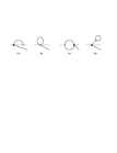
Figure 2: $K\to\pi\pi$ one-loop contributions.

4.2 Comparison with Unitarization Procedures

The possible impact of final-state interactions (FSI) on weak transition amplitudes has recently drawn attention in the literature. [12, 13] Using the work of Ref. [12] as an example, the $K\to(\pi\pi)_{I}$ amplitude induced by the usual nonleptonic weak interaction is written in the form

$${\cal A}_{I}(s)={\cal A}_{I}^{(0)}(s-m_{\pi}^{2})e^{i\delta_{0}^{I}(s)}{\cal R}_{I}(s)\ \ ,$$ (42)

where ${\cal A}_{I}^{(0)}$ is the derivative of ${\cal A}_{I}$ at the point $s=m_{\pi}^{2}$ and ${\cal R}_{I}(s)$ is a dispersive corection factor. The above form is an Omnès-type solution which includes the effect of final-state rescattering. In the approximation of including just the two-pion final states, Ref. [12] obtains for the $I=0,2$ rescattering corrections

$${\cal R}_{0}(m_{K}^{2})=1.41\pm 0.06\ ,\qquad{\cal R}_{2}(m_{K}^{2})=0.92\pm 0.02\ \ .$$ (43)

This means that, within errors, the effect of final state interactions enhances the $I=0$ amplitude by $41\%$ and suppresses the $I=2$ amplitude by $8\%$. It is revealing to compare these FSI effects with our ${\cal O}(p^{2})$ fractional corrections $\Delta_{0}$ and $\Delta_{2}$ given in Eq. (41). Our finding that $\Delta_{0}$ is large and positive is in qualitative accord with the above value for ${\cal R}_{0}(m_{K}^{2})$, but our positive value for $\Delta_{2}$ conflicts with the suppression implied by ${\cal R}_{2}(m_{K}^{2})$.

The resolution of this apparent paradox lies in a more careful comparison of the two approaches. In Fig. 2(a)-(d), we display the four distinct one-loop contributions to our $K\to\pi\pi$ electroweak penguin matrix elements. The contribution of Fig. 2(c) (the ‘back-facing swordfish’) is the only one with a two-pion intermediate state and is the only contribution whose iteration would occur in an Omnès-type resummation. A calculation of the fractional shift induced by Fig. 2(c) yields

$$\Delta_{0}^{2(c)}=0.36\pm 0.12\ ,\qquad\qquad\Delta_{2}^{2(c)}=-0.15\pm 0.05\ \ .$$ (44)

Both these values are in reasonable agreement with those implied by Eq. (43). It is the other contributions in Fig. 2 (which we emphasize are demanded by the stringent requirements of chiral symmetry) which are dominant and which determine the overall sign of $\Delta_{2}$.

5 Conclusion

The calculation of matrix elements of local operators which enter the $\Delta S=1$ weak effective hamiltonian is a crucial step in the phenomenology of nonleptonic kaon decays. In this paper we have focussed on some general aspects of the ${\cal O}(p^{2})$ corrections to the electroweak penguin operators ${\cal Q}_{7,8}$. Our results can be summarized as follows:

1. Direct calculational methods (such as lattice-QCD, chiral sum rules, large-$N_{c}$ QCD) usually deal with the simpler $K\rightarrow\pi$ transitions and rely on chiral symmetry relations to infer the physical $K\rightarrow\pi\pi$ matrix elements. Although trivial in leading order (which is ${\cal O}(p^{0})$ in this case), these relations become more involved at next-to-leading order in the chiral expansion. We have systematically worked out the form of the $K\rightarrow\pi$ and $K\rightarrow\pi\pi$ matrix elements at ${\cal O}(p^{2})$ in the framework of ChPT, including one-loop diagrams and local counterterms (as required by power counting). We find that knowledge of the $K\rightarrow\pi$ matrix elements is generally enough to fully determine the low energy constants entering in the $K\rightarrow\pi\pi$ matrix elements. Thus all chiral studies of this system, analytic or lattice-QCD, can safely use the $K\to\pi$ mode to infer properties of the $K\to\pi\pi$ system.

2. We have used background-field and heat-kernel techniques to perform the renormalization of the one-loop effective action in the presence of an insertion of the generic ${\bf 8}_{L}\times{\bf 8}_{R}$ operators ${\cal O}_{ab}$ of Eq. (5). Although the results given in Eqs. (22),(24) pertain specifically to the electroweak penguin operator of Eq. (4), the procedure is easily generalized to applications involving other left-right operators. The divergent counterterm coefficients predicted by the general heat-kernel approach are in complete agreement with the divergences explicitly found in our one-loop calculation and thus provide a check on the calculation.

3. Another important aspect of our work is the ‘chiral-loop’ estimate of the ${\cal O}(p^{2})$ correction to $\langle(\pi\pi)_{I}|{\cal Q}_{7,8}|K\rangle$ (cf Eq. (41)). On a qualitative level, we have answered the question of whether the corrections might be anomalously small (${\cal O}(m_{\pi}^{2})$) due to the absence of ${\cal O}(m_{K}^{2})$ contributions. For example, recall that electromagnetic corrections to the $K^{+}\rightarrow\pi^{+}\pi^{0}$ matrix element of the octet weak lagrangian contains only small ${\cal O}(\alpha m_{\pi}^{2})$ corrections even though the larger ${\cal O}(\alpha m_{K}^{2})$ terms are allowed by power counting and symmetry arguments. We have found here that ${\cal O}(m_{K}^{2})$ effects are not absent. This is why the leading-log result exhibits a strong dependence on the chiral scale $\mu_{\chi}$. Our analysis cannot, therefore, exclude the possibility of important corrections to the chiral determination.

   More quantitatively, we obtain the large ${\cal O}(p^{2})$ correction $\Delta_{0}=0.98\pm 0.55$ in the isospin-zero two-pion channel. It is not surprising that this agrees with Omnès-type resummation procedures [12, 13] because strong rescattering effects are expected to play an important role for the $I=0$ channel. Of greater interest is the $I=2$ two-pion channel, since it bears on attempts to predict $\epsilon^{\prime}/\epsilon$. Here, the situation is more subtle. The fractional correction $\Delta_{2}=0.27\pm 0.27$ is moderate in magnitude and positive in sign. The sign of $\Delta_{2}$ is opposite to that obtained in an Omnès-type resummation approach. As explained in Sect. 4.2 this is attributable to ${\cal O}(p^{2})$ contributions not included in the unitarized amplitudes. The underlying lesson is that unitarization of a part of the full amplitude can lead to valid results when rescattering is strong but can be misleading when rescattering is weak.

This work represents a preliminary but necessary step towards a fully predictive analysis of the matrix elements $\langle\pi\pi|{\cal Q}_{7,8}|K\rangle$ beyond the chiral limit. Work is underway to extend the dispersive analysis carried out in Ref. [2] to the general case of $m_{\rm quark}\neq 0$.

The research described here was supported in part by the National Science Foundation. One of us (V.C.) acknowledges support from M.U.R.S.T. We thank John Donoghue for useful comments on this work.

References

- [1] A. Alari-Harati et. al (KTeV collaboration), Phys. Rev. Lett. 83 (1999) 22; G. Barr, Plenary talk at XIX Intl. Symp. on Lepton-Photon Interactions at High Energies, Stanford University, 8/7/99-8/14/99.
- [2] J.F. Donoghue and E. Golowich, ‘Dispersive calculation of and in the chiral limit’, Univ. of Massachusetts preprint, hep-ph/9911309; see also M.Knecht, S.Peris, E.de Rafael, Phys.Lett.B457 (1999), 227.
- [3] A. Donini, V. Gimenez, L. Giusti and G. Martinelli, Delta(S) = 2 and Delta(I) = 3/2 four-fermion operators without quark masses,” hep-lat/9910017.
- [4] J.Bijnens, H.Sonoda, M.B.Wise, Phys.Rev.Lett. 53 (1984), 2367.
- [5] C.Bernard, T.Draper, A.Soni, H.D.Politzer, M.B.Wise, Phys.Rev.D32 (1985), 2343
- [6] J.Bijnens, Phys.Lett.B152 (1985), 226.
- [7] J.Bijnens, E.Pallante, J.Prades, Nucl.Phys.B521 (1998),305.
- [8] J.F. Donoghue, E. Golowich and B.R. Holstein, Dynamics of the Standard Model, (Cambridge University Press, Cambridge, England 1992).
- [9] J. Gasser and H. Leutwyler, Ann. Phys. 158 (1984) 142.
- [10] J. Gasser and H. Leutwyler, Nucl. Phys. B250 (1985) 465.
- [11] R.J. Crewther, Nucl. Phys. B264 (1986) 277.
- [12] Strong enhancement of through final state interactions, E. Pallante and A. Pich, Univ. de Barcelona preprint, hep-ph/9911233 v2.
- [13] Rescattering effects for , E. Paschos, Univ. Dortmund preprint, hep-ph/9912230 v2.
- [14] Electromagnetic Corrections to I – Chiral Perturbation Theory, V. Cirigliano, J.F. Donoghue and E. Golowich, Phys. Rev. D (to be published), hep-ph/9907341.