Spinodal Decomposition and Inflation: Dynamics and Metric Perturbations

Abstract

We analyse the dynamics of spinodal decomposition in inflationary cosmology using the closed time path formalism of out of equilibrium quantum field theory combined with the non-perturbative Hartree approximation. In addition to a general analysis, we compute the detailed evolution of two inflationary models of particular importance: $\lambda\Phi^{4}$ new inflation and natural inflation. We compute the metric fluctuations resulting from inflationary phase transitions in the slow roll approximation, showing that there exists a regime for which quantum fluctuations of the inflaton field result in a significant deviation in the predictions of the spectrum of primordial density perturbations from standard results. We provide case examples for which a blue tilt to the power spectrum (i.e. $n_{s}>1$) results from the evolution of a single inflaton field, and demonstrate that field fluctuations may result in a scalar amplitude of fluctuations significantly below standard predictions, resulting in a slight alleviation of the inflationary fine tuning problem. We show explicitly that the metric perturbation spectrum resulting from inflation depends upon the state at the outset of the inflationary phase.

I Introduction

In recent years, there has been a strong interest in the dynamics of quantum fields in the early universe. This interest has led to a better understanding of a number of processes including the formation of topological defects during early phase transitions[1], the reheating of the universe after inflation[2], and the dynamics of inflation itself[3]. In the particular case of inflationary reheating, our improved understanding has been revolutionary and has significantly reshaped the subject[4].

The lessons provided by these studies are varied. One crucial aspect is the importance of using time-dependent techniques to study processes of the early universe. It has been repeatedly shown that classical and one-loop effective potentials are poorly defined and of little use in dynamical systems; they should only be used to determine static quantities such as the ground state of the system[5]. Another common theme is the importance of non-linear corrections to the linear dynamics. These corrections have been found to be quite dramatic in studies of phase transitions and reheating.

Despite these important advances in studies of quantum fields in the early universe, it is still widely believed that these techniques have little to add to our understanding of the inflationary phase itself. The belief that the inflaton follows a classical trajectory determined from the classical effective potential with only perturbatively small quantum corrections[6] is still widely held. While the techniques of stochastic inflation[7] allow these corrections to add up, they do so in an incoherent fashion through a repeated summation of one-loop effects without self-consistent inclusion of higher order corrections[8].

Much work has been done to verify that the dynamics of the inflaton field is predominantly classical. The existence of a particle horizon and the natural squeezing of states due to the near exponential redshifting of field modes justifies a quasi-classical description of the inflaton field up to a perturbatively small component of field fluctuations with wavelengths inside the de Sitter horizon[9]. However, it is important to emphasize that the validity of a classical evolution of the inflaton field alone does not justify the use of the classical effective potential for a non-linear dynamical system. As has been shown quite clearly by the classical field theory simulations of the early stages of reheating, the full non-linear dynamics of even a purely classical system depends strongly on coherent effects of backreaction due to the field’s fluctuations[10]. It is then not unreasonable to expect that non-linear field fluctuations during inflation could result in a departure from the dynamics derived directly from the classical effective potential.

In this report we address these issues using the techniques of out-of-equilibrium quantum field theory. We examine a class of models in which strongly quenched inflaton evolves under the influence of a negative mass squared in the potential, a process which, following the terminology of such phase transitions in condensed matter physics, we refer to as spinodal decomposition[11]. This class of inflation models includes new[12] and natural inflation[13], as well as many models of hybrid inflation[14]. Such inflation models are of particular interest in the present study because the evolution from the initial to the final state of the system is necessarily a non-linear process.

The particular case in which the inflaton field is treated as a component of an $O(N)$ vector in the large $N$ limit has already been detailed for the case of new inflation, where it was found that the full non-perturbative quantum dynamics does in fact reproduce an effectively classical trajectory for the evolution of the inflaton. The growth of quantum fluctuations results in a dynamical flattening of the potential[15], an analogue of the Maxwell construction commonly used in studies of the equilibrium properties of phase transitions. In this earlier work, it was found that the effectively classical trajectory of the inflaton field, a result of the phenomenon known as zero mode reconstruction, is a consequence of Goldstone’s theorem[16].

However, the case of a single, real inflaton field is quite different. Here, the long wavelength quantum fluctuations of the field also reassemble themselves into a semi-classical field, but in this case the assembled field does not obey the classical equations of motion of the original potential. Rather, the inflaton may be broken up into two components. The first is the mean field $\phi$ and obeys the classical equation of motion expected from the original potential except that it is coupled to a second field. This second field $\sigma$, constructed through the assembly of quantum fluctuations, obeys a modified equation of motion. The result is an effectively classical theory of two coupled fields, refered to as spinodal inflation[17].

The observational consequences are dramatic. As there are effectively two fields, the evolution becomes quite complicated and depends on the initial conditions. There are two regimes. In the first, the mean inflaton field, defined as the expectation value of the quantum field, has an initial value greater than the expansion rate $\phi(t_{0})>H_{0}/2\pi$ and the semi-classical field $\sigma$ never becomes dynamically relevant. The evolution reproduces all of the standard results for that particular model of inflation and we can think of this as the classical regime. In the second, quantum, regime for which $\phi(t_{0})<H_{0}/2\pi$, the influence of the $\sigma$ field is quite important. In this case, observational quantities such as the amplitude and spectrum of primordial density fluctuations depend not only on the parameters of the model, but also on the particular value of the initial mean field $\phi(t_{0})$.

A simple single field model can therefore produce a range of observational results for any given choice of parameters. In fact, due to the effective two field dynamics, it is possible to produce observational features not possible in the simple classical, single field version of the same theory, such as the generation of a blue primordial power spectrum; this can occur much in the same way as it does in hybrid inflation.

We begin with a short introduction to spinodal models of inflation and the need for a fully out-of-equilibrium and non-perturbative description of the dynamics. We write down the self-consistent Hartree equations of motion for a general spinodal potential, followed by an explanation of the assembly of quantum fluctuations and how this results in an effectively classical two field model. Next, we move on to a detailed analysis of the two most important spinodal models of inflation, $\lambda\Phi^{4}$ new inflation and natural inflation.

Having determined the evolution of the field, we wish to examine the observational consequences of spinodal inflation. Beginning with the gauge invariant formulation of gravitational perturbations of Mukhanov, Feldman, and Brandenberger[18], we note that while the effective dynamics is that of two fields, returning to the full quantum theory we see that only one set of field fluctuations couples to gravity perturbations.

We then provide a complete and detailed numerical analysis of the dynamics of spinodal inflation in single field models, including computations of the primordial spectrum of scalar and tensor perturbations which result. The consequent $C_{l}$ spectra[19] for a particularly interesting example is shown to allow for the direct relation of spinodal effects to observation. Here we see explicitly the exciting features possible through the dynamics of spinodal inflation.

II Spinodal models of inflation

We envision the evolution of a scalar field near the top of a potential of the form sketched in Fig. 1. The potential may be expanded in the form

$$V(\Phi)=K-\frac{1}{2}\mu^{2}\Phi^{2}+\frac{\lambda}{4!}\Phi^{4}+\cdots\;,$$ (1)

where the cosmological constant contribution $K$ is chosen such that the potential is zero in the true vacuum, and $\mu^{2}$ is positive.

Initially, the field will “roll” slowly toward one of the minima of the potential. This is the regime in which inflation will take place. To a first approximation, we ignore the quartic term and see that the initial evolution follows that of a free field in an inverted harmonic potential. This evolution has been studied in great detail in the context of inflationary cosmology[20]. For early times, the field grows exponentially. Eventually the higher order terms in the potential become important, with the result that any perturbative analysis of the dynamics will break down and must be augmented by some non-perturbative technique.

Our choice of approximation is further restricted by the fact that the system we wish to study is not in thermal equilibrium, thus leading us to real-time methods. We emphasize that equilibrium constructs, such as the effective potential, are completely inadequate tools for this problem.

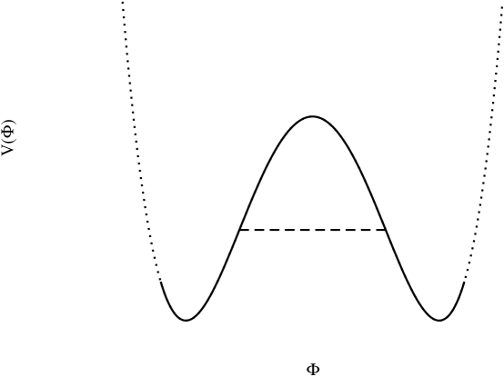
FIG. 1.: A typical potential with a region of negative curvature. The dashed line is the spinodal line, separating the unphysical spinodal region (above the line) from the physical region (at and below the line). The exact shape of the dotted portion of the curves depends upon the higher order terms in Eq. (1).

The simplest approximation satisfying the requirements is the Gaussian variational approximation, in which the quantum density matrix is restricted to take on a Gaussian form. Also known as the Time Dependent Hartree-Fock approximation, such mean field techniques have been utilized in quantum mechanics dating back to Dirac[21]. It is a standard technique in chemistry, condensed matter physics, and nuclear physics and has led to a better understanding of the structure of a number of phase transitions.

A Real Scalar Field: Hartree Dynamics

In what follows, we assume a spatially flat Robertson-Walker metric:

$$ds^{2}=dt^{2}-a^{2}(t)d\vec{x}^{2}\;.$$ (2)

We now derive the equations of motion for a real scalar field with Lagrangian

$$L=\frac{1}{2}\nabla^{\mu}\Phi(x)\nabla_{\mu}\Phi(x)-V\left[\Phi(x);t\right]\;,$$ (3)

within the self-consistent Hartree approximation[22]. We break up the field $\Phi$ into its expectation value plus a fluctuation about this value:

$$\Phi(\vec{x},t) = \phi(t)+\psi(\vec{x},t)\;,$$ (4)

$$\phi(t) \equiv \langle\Phi(\vec{x},t)\rangle\;.$$ (5)

Here, $\phi$ depends only on time due to space translation invariance as is consistent with the metric (2). By definition $\langle\psi(\vec{x},t)\rangle=0$.

The Hartree approximation consists of replacing $\psi^{2n}$ by $c_{1}\langle\psi^{2}\rangle^{n-1}\psi^{2}+c_{2}\langle\psi^{2}\rangle^{n}$ and $\psi^{2n+1}$ by $c_{3}\langle\psi^{2}\rangle^{n}\psi$, where the $c_{i}$ are constant factors whose values are determined by Wick’s Theorem. This Hartree factorization may be summarized as follows:

$$\psi^{2n} \to \frac{(2n)!}{2^{n}(n-1)!}\langle\psi^{2}\rangle^{n-1}\psi^{2}-\frac{(2n)!(n-1)}{2^{n}n!}\langle\psi^{2}\rangle^{n}\;,$$ (6)

$$\psi^{2n+1} \to \frac{(2n+1)!}{2^{n}n!}\langle\psi^{2}\rangle^{n}\psi\;.$$ (7)

Given this factorization, any function $F(\Phi)$ becomes

$$F(\phi+\psi)=\sum_{n=0}^{\infty}\frac{1}{n!}\left(\frac{\langle\psi^{2}\rangle}{2}\right)^{n}\left\{F^{(2n)}(\phi)+\psi F^{(2n+1)}(\phi)+\frac{1}{2}\left[\psi^{2}-\langle\psi^{2}\rangle\right]F^{(2n+2)}(\phi)\right\},$$ (8)

where we use the notation

$$F^{(n)}(\phi)\equiv\frac{\delta^{n}}{\delta\phi^{n}}F(\phi)\;.$$ (9)

Note that the latter two terms on the right hand side of Eq. (8) have zero expectation value. We therefore find that the expectation value of a function factorizes as

$$\langle F(\phi+\psi)\rangle=\sum_{n=0}^{\infty}\frac{1}{n!}\left(\frac{\langle\psi^{2}\rangle}{2}\right)^{n}F^{(2n)}(\phi)\;.$$ (10)

The equations of motion for the mean field $\phi$ are given by the tadpole condition $\langle\psi\rangle=0$ [23]:

$$\ddot{\phi}(t)+3\frac{\dot{a}(t)}{a(t)}+\sum_{n=0}^{\infty}\frac{1}{n!}\left(\frac{\langle\psi^{2}\rangle}{2}\right)^{n}V^{(2n+1)}(\phi)=0\;,$$ (11)

where we have used the metric (2) and have factorized the expectation value $\langle V^{{}^{\prime}}(\Phi)\rangle$ according to Eq. (10). We define the Fourier transform of the Wightman function by the expression

$$G(\vec{x},t;\vec{x}^{{}^{\prime}},t^{{}^{\prime}})=\int\frac{d^{3}k}{(2\pi)^{3}}e^{i\vec{k}\cdot(\vec{x}-\vec{x}^{{}^{\prime}})}G_{k}(t,t^{{}^{\prime}})\;,$$

where we have used the property of space translation invariance. The quantity $\langle\psi^{2}(t)\rangle\equiv-iG(x,x)$ is constructed from the mode functions obeying the equation

$$[G_{k}(t,t)]^{-1}f_{k}(t)=0\;,$$ (12)

together with the appropriate Closed Time Path boundary conditions[24]. The operator $[G_{k}]^{-1}$ is given by the quadratic form appearing in the generating functional. Explicitly, the $f_{k}(t)$ obey

$$\left[\frac{d^{2}}{dt^{2}}+3\frac{\dot{a}(t)}{a(t)}\frac{d}{dt}+\frac{k^{2}}{a^{2}(t)}+\sum_{n=0}^{\infty}\frac{1}{n!}\left(\frac{\langle\psi^{2}\rangle}{2}\right)^{n}V^{(2n+2)}(\phi)\right]f_{k}(t)=0\;,$$ (13)

where we have again used the factorization (10) to express the potential term $\langle V^{{}^{\prime\prime}}(\Phi)\rangle$.

As mentioned above, the quantity $\langle\psi^{2}\rangle$ is determined from the mode functions $f_{k}$ combined with Closed Time Path boundary conditions appropriate to the chosen initial state. For an initial state in thermal equilibrium at an initial temperature $T$, we have

$$\langle\psi^{2}(t)\rangle=\int\frac{d^{3}k}{(2\pi)^{3}}|f_{k}(t)|^{2}\coth\left(\frac{\omega_{k}}{2T}\right)\;,$$ (14)

Note that in the zero temperature vacuum state given by the $T\to 0$ limit, the hyperbolic cotangent has the value $1$. The frequency $\omega_{k}$ appearing here is given by

$$\omega_{k}^{2}=k^{2}+a^{2}(t_{0})\sum_{n=0}^{\infty}\frac{1}{n!}\left(\frac{\langle\psi^{2}(t_{0})\rangle}{2}\right)^{n}V^{(2n+2)}(\phi(t_{0}))\;.$$ (15)

For the case of the $\lambda\Phi^{4}$ theory, there is an additional term proportional to the Ricci scalar $-a^{2}(t_{0})R(t_{0})/6$ which appears on the right hand side of this expression for $\omega_{k}$. This term arises when one considers initial conditions corresponding to the adiabatic vacuum state in conformal time[25, 26], which is necessary if we wish our initial vacuum state to match the Minkowski vacuum in the limit $a(t)\to 1$. However, this term is not necessary if the scalar field is taken to be part of a low energy effective theory, such as is the case with the natural inflation case we analyze below.

Using the vacuum state for the mode functions defined by the initial frequency spectrum of Eq. (15) leads to the following initial conditions on the $f_{k}(t)$:

$$f_{k}(t_{0}) = \frac{1}{\sqrt{2\omega_{k}}}\;,$$ (16)

$$\dot{f}_{k}(t_{0}) = \left(-\frac{\dot{a}(t_{0})}{a(t_{0})}-i\omega_{k}\right)f_{k}(t_{0})\;.$$ (17)

A final note is that the initial frequencies $\omega_{k}$ given by Eq. (15) may be imaginary for low $k$ modes. In this case the initial conditions (17) need to be modified for low $k$. This may be done in a variety of ways with little effect on results[16]. Here, we choose a smooth interpolation between low $k$ modes with modified frequencies and the high $k$ modes which remain in the conformal vacuum state with frequencies $\omega_{k}$ (15):

$$\omega_{k}^{2}\equiv k^{2}+{\cal{M}}^{2}\tanh\left(\frac{k^{2}+{\cal{M}}^{2}}{|{\cal{M}}^{2}|}\right)\;,$$ (18)

where

$${\cal M}^{2}\equiv a^{2}(t_{0})\sum_{n=0}^{\infty}\frac{1}{n!}\left(\frac{\langle\psi^{2}(t_{0})\rangle}{2}\right)^{n}V^{(2n+2)}(\phi(t_{0}))\;.$$ (19)

This completes our set of equations of motion of the matter fields within the Hartree approximation.

B Gravitational Dynamics

We will treat gravity in the semi-classical approximation, in which the expectation value of the full quantum energy-momentum tensor acts as a classical source to the Einstein gravitational tensor. The semi-classical Einstein’s equation reads

$$\frac{G^{\mu}_{\nu}}{8\pi G_{N}}+\frac{\Lambda}{8\pi G_{N}}+\left({\rm higherderivatives}\right)=-\langle T^{\mu}_{\nu}\rangle\;,$$ (20)

where $G_{N}=1/M_{Pl}^{2}$ is (bare) Newton’s constant, $\Lambda$ is the (bare) cosmological constant and the components of the Einstein curvature tensor using the metric (2) are:

$$G^{0}_{0} = -3\frac{\dot{a}^{2}}{a^{2}}\;,$$ (21)

$$G^{\mu}_{\mu} = -R=-6\left(\frac{\ddot{a}}{a}+\frac{\dot{a}^{2}}{a^{2}}\right)\;.$$ (22)

The higher derivative terms included in Eq.(20) are needed for renormalization purposes; Newton’s constant and the cosmological constant will also be renormalized (see below).

Once again, we use the factorization (10) to determine the right hand side of (20). Defining the additional integrals

$$\langle\dot{\psi}^{2}(t)\rangle = \int\frac{d^{3}k}{(2\pi)^{3}}|\dot{f}_{k}(t)|^{2}\coth\left(\frac{\omega_{k}}{2T}\right)\;,$$ (23)

$$\langle(\vec{\nabla}\psi(t))^{2}\rangle = \int\frac{d^{3}k}{(2\pi)^{3}}k^{2}|f_{k}(t)|^{2}\coth\left(\frac{\omega_{k}}{2T}\right)\;,$$ (24)

we find for the energy density $\varepsilon$ and the trace ${\cal T}$ of the energy momentum tensor:

$$\varepsilon = \langle T^{0}_{0}\rangle=\frac{1}{2}\dot{\phi}^{2}+\frac{1}{2}\langle\dot{\psi}^{2}\rangle+\frac{1}{2a^{2}}\left\langle(\vec{\nabla}\psi)^{2}\right\rangle+\sum_{n=0}^{\infty}\frac{1}{n!}\left(\frac{\langle\psi^{2}\rangle}{2}\right)^{n}V^{(2n)}(\phi)\;,$$ (25)

$${\cal T} = \langle T^{\mu}_{\mu}\rangle=-\dot{\phi}^{2}-\langle\dot{\psi}^{2}\rangle+\frac{1}{a^{2}}\left\langle(\vec{\nabla}\psi)^{2}\right\rangle+4\sum_{n=0}^{\infty}\frac{1}{n!}\left(\frac{\langle\psi^{2}\rangle}{2}\right)^{n}V^{(2n)}(\phi)\;.$$ (26)

The pressure $p$ is arrived at from these expressions through the relation $p=(\varepsilon-{\cal T})/3$. The equation of state of the system is characterized by the quantity $w=p/\varepsilon$.

C Regularization and Renormalization

The mode integrals appearing in Eq. (14), (23), and (24) are formally divergent and must be regularized in order to perform any practical computation.

In the special case of a renormalizable potential $V(\Phi)$, for example in the $\lambda\Phi^{4}$ model, we would like to fully renormalize the theory. Our choice of renormalization procedures is somewhat limited by the requirement that the dynamics be amenable to numerical analysis. However, a number of groups have recently addressed this problem either by means of adiabatic regularization with a simple cutoff at large momentum[27, 25, 28], as was first developed by Paul Anderson[29], or by using a scheme based on dimensional regularization[30].

In practice, we use the simple scheme developed by the Pittsburgh-Paris collaboration. This scheme has the advantage of being very easy to implement and it has the attractive feature that all subtractions are absorbed into counterterms renormalizing the bare couplings in the equation of motion and the Friedmann equation (the latter must be extended to include a cosmological constant and a higher order curvature term). However, we mention that it does not include the finite subtractions which would be necessary to give the correct conformal anomaly. These terms, the finite subtractions detailed in [27] and [28], are formally important, but in the present context, as the inflaton self-coupling is typically required to be of order $10^{-12}$ or smaller, such terms will have absolutely no influence on numerical simulations as their contributions are much smaller than the numerical accuracy of the computations. In fact, although we do not do so here, it is normally safe to drop the logarithmically divergent terms from the simulations as well without influencing the results. The simulations are checked after the fact to verify that they satisfy the covariant conservation of the energy-momentum to within their numerical accuracy, and to ensure that the results are independent of the value of the momentum cutoff.

For models with non-renormalizable potentials, such as natural inflation, we have to satisfy ourselves with the treatment of the model as a low energy effective theory with a well defined cutoff. Again, we implement the regularization by means of a large momentum cutoff.

III Early Time Dynamics and Reassembly

As mentioned above, the initial linear dynamics in spinodal models of inflation is well understood. This period is characterized by exponential growth of both the mean field $\phi$ and those mode functions $f_{k}$ with physical wavelength greater than the Hubble distance, that is, $k/a(t)\ll H(t)\equiv\dot{a}(t)/a(t)$. Since $H(t)$ is approximately constant during inflation while $a(t)$ is growing exponentially, clearly more and more modes satisfy this condition at each subsequent time. However, the very long wavelength modes which crossed the horizon very early on in the evolution will tend to dominate the quantity $\langle\psi^{2}\rangle$ of Eq. (14) simply because they have experienced the spinodal instability for the longest time. This is a very important characteristic of spinodal inflation which sets it apart from other models: the dynamics is driven by a super-horizon scale quasi-particle condensate. On scales smaller than the horizon, it is not possible to distinguish such a condensate from a purely homogeneous background field. Any possible measurement will determine only the combined properties of the condensate and the mean field.

Given the assumption of initial conditions near the local maximum of the potential, and provided with a finite renormalized or regularized two-point function along with very small values for the higher order couplings in the Lagrangian, the early dynamics is well approximated by a linear analysis. The equation for the mean field for any potential of the form (1) is simply

$$\ddot{\phi}(t)+3H(t)\dot{\phi}(t)-\mu^{2}\phi(t)=0\;.$$ (27)

To this order, we may take the Hubble parameter to be constant, $H(t)=H_{0}$, in which case the solutions to this equation are simple exponentials. Only the growing term is relevant, so that we have the early time solution

$$\phi(t)\approx\phi_{0}\exp\left[\left(\nu-\frac{3}{2}\right)H_{0}t\right]\quad\quad\nu=\sqrt{\frac{9}{4}+\frac{\mu^{2}}{H_{0}^{2}}}\;.$$ (28)

The value of $\phi_{0}$ depends on the precise initial conditions for $\phi$ and $\dot{\phi}$.

The mode functions obey the similar equation

$$\ddot{f}_{k}(t)+3H(t)\dot{f}_{k}(t)+\left(\frac{k^{2}}{a^{2}(t)}-\mu^{2}\right)f_{k}(t)=0\;,$$ (29)

which for constant $H(t)=H_{0}$ and corresponding exponential $a(t)=\exp(H_{0}t)$ has the solutions

$$f_{k}(t)\approx\exp\left(-\frac{3}{2}H_{0}t\right)\left[A_{k}J_{\nu}\left(\frac{k}{H_{0}}e^{-H_{0}t}\right)+B_{k}J_{-\nu}\left(\frac{k}{H_{0}}e^{-H_{0}t}\right)\right]\;.$$ (30)

The constants $A_{k}$ and $B_{k}$ are determined by the initial conditions on the mode functions. These solutions oscillate with an envelope proportional to $1/a$ for sub-horizon modes (with $k/a>H_{0}$), but the solutions are growing and decaying exponentials in the opposite limit $k/a\ll H_{0}$, leading to the statement that super-horizon modes have an exponential instability. In this limit, we may again discard the exponentially decaying term. We then have for super-horizon modes

$$f_{k\ll aH}(t)\approx\frac{C_{k}}{k^{\nu-3/2}}\exp\left[\left(\nu-\frac{3}{2}\right)H_{0}t\right]\;.$$ (31)

Here, $C_{k}$ is roughly equal to the value of the mode $f_{k}$ evaluated at the time $t(k)$ that the mode crosses the horizon as determined by the condition $k=\exp[H_{0}t(k)]H_{0}$. For modes initially far within the horizon the general dependence of $C_{k}$ on $k$ may be estimated from the initial behavior of the mode functions $f_{k}\sim k^{-1/2}$ and the decay of the envelope of the Bessel solutions which provides the standard result that $C_{k}\propto k^{-3/2}$. We note that while the exponential form (31) is only an asymptotic solution for small arguments of the Bessel functions of Eq. (30), due to the exponential behavior of this argument it very accurately describes the evolution any mode function within a Hubble time of horizon crossing.

We are now in position to compute an expression for the condensate $\langle\psi^{2}\rangle$. By separating the momentum space integral over super- and sub-horizon modes respectively, we can take advantage of the expression (31) to find for early times

$$\langle\psi^{2}\rangle=\exp\left[\left(\nu-\frac{3}{2}\right)H_{0}t\right]\int_{0}^{aH}\frac{d^{3}k}{2(2\pi)^{3}}\frac{|C_{k}|^{2}}{k^{2\nu-3}}+\langle\psi^{2}\rangle_{k>aH}\;.$$ (32)

The latter, sub-horizon term contains all subtractions due to renormalization. After a few Hubble times, it is safe to neglect this term compared to the exponentially growing super-horizon contribution. To determine which modes are most important to the evolution, it is convenient to examine the contribution of each squared mode per logarithmic momentum interval, $dk/k$. Using the $k^{-3/2}$ behavior of $C_{k}$, we find for modes which are originally far inside the horizon, but which have since crossed outside, that this contribution is proportional to $k^{-(2\nu-3)}$. Since $2\nu>3$, the integral is dominated by those modes which crossed the horizon the earliest. This is important for any numerical analysis as it allows one in practice to set a cutoff in the calculation of $\langle\psi^{2}\rangle$ with well controlled errors, avoiding the problem of including a number of mode functions which grows exponentially with the scale factor.

As a consequence of the formation of the condensate, it becomes possible to form an accurate and simple model of the complete system, in which the full two-point fluctuation $\langle\psi^{2}\rangle$ is replaced by a nearly homogeneous, and effectively classical field. This produces a model in which two effectively homogeneous classical fields, the mean field coupled to a fluctuation field, accurately describe the dynamics. The condensate field is defined as

$$\sigma(t)\equiv\sqrt{\langle\psi^{2}(t)\rangle_{k<aH}}\;.$$ (33)

For early times, it is given by the first term on the right hand side of Eq. (32). The square root of the value of the first integral of (32) a few Hubble times after the beginning of inflation provides an effective initial condition on $\sigma$. For a zero temperature initial state, which for simplicity we take to be the case in what follows, this is found numerically to be of order $H/2\pi$[16]. The effect of a finite temperature initial state is to increase this value by a factor of $\sqrt{T/\mu}$ without modifying any of the qualitative features described in this study. The dynamics modelled by this classical field will be accurate up to perturbatively small corrections to the dynamics due to the sub-horizon modes contained in the final term of Eq. (32).

This system of effective homogeneous fields is referred to as a reassembled system. We will refer to the $\phi$ field, the expectation value of the full quantum field, as the mean field, while we refer to the semi-classical $\sigma$ field as the fluctuation or condensate field.

While this condensate forms during the linear regime, eventually the dynamics becomes non-linear. It is this non-linear evolution which we wish to study. We will be particularly interested in examining how the interaction of the condensate with the mean field can influence the dynamics.

We consider primarily the dynamics of single field models (the large $N$ case was studied previously[16]). Here, the interactions of the condensate and the mean field will be seen to lead to a complicated evolution in which initial conditions play a primary role.

IV Non-linear Dynamics

We begin with an analysis of the stationary solutions for the mean field, which obeys the equation of motion (11). There are two primary late time solutions. The first is the trivial solution with $\phi(t)=0$, which will be the solution for a system without symmetry breaking. The other solution, relevant for spinodal inflation, is given by the condition

$$\left\langle V^{\prime}\left(\phi(t)+\psi(\vec{x},t)\right)\right\rangle_{a}=\sum_{n=0}^{\infty}\frac{1}{n!}\left(\frac{\langle\psi^{2}\rangle_{a}}{2}\right)^{n}V^{(2n+1)}(\phi_{a})=0\;,$$ (34)

where the subscript $a$ indicates the asymptotic solution. Unlike the sum rule in the large $N$ limit[16], this condition does not correspond to massless field modes[31]. Rather, for a bounded potential of the form (1) with a definite minimum at finite values for $\Phi$, the effective mass of particle modes appearing in (13) will be positive. Asymptotically, we therefore expect the field modes to be redshifted away due to expansion of the universe such that the quantity $\langle\psi^{2}\rangle$ becomes small and may be neglected in (34). In this case, the expression for the stationary solution becomes simply

$$V^{\prime}(\phi_{a})=0\;,$$ (35)

and the effective mass of the field modes is

$$M^{2}_{eff}=V^{\prime\prime}(\phi_{a})\;.$$ (36)

These, of course, are just the classical vacuum solutions in the symmetry broken phase.

The task is to connect the early time solutions of Eqs. (28) and (30) and the late time solutions provided by Eqs. (35) and (36). It is convenient to introduce the effective condensate field defined as in (33). Doing so, and neglecting the exponentially suppressed gradient term in the expression for the energy density (25), leads to the following equations of motion for the mean field $\phi$, the condensate field $\sigma$, and the scale factor $a$:

$$\ddot{\phi}+3\frac{\dot{a}}{a}\dot{\phi}+\sum_{n=0}^{\infty}\frac{1}{2^{n}n!}\sigma^{2n}V^{(2n+1)}(\phi) = 0\;,$$ (37)

$$\ddot{\sigma}+3\frac{\dot{a}}{a}\dot{\sigma}+\sum_{n=0}^{\infty}\frac{1}{2^{n}n!}\sigma^{2n+1}V^{(2n+2)}(\phi) = 0\;,$$ (38)

$$\frac{\dot{a}^{2}}{a^{2}}=\frac{8\pi G_{N}}{3}\left[\frac{1}{2}\dot{\phi}^{2}+\frac{1}{2}\dot{\sigma}^{2}+\sum_{n=0}^{\infty}\frac{\sigma^{2n}}{2^{n}n!}V^{(2n)}(\phi)\right]\;.$$ (39)

Remarkably, these equations are just those one would derive from a classical system of two homogeneous fields with the potential

$$V(\phi,\sigma)=\sum_{n=0}^{\infty}\frac{1}{2^{n}n!}\sigma^{2n}V^{(2n)}(\phi)\;.$$ (40)

An important property of this potential is that, for interacting fields, it does not depend symmetrically upon $\phi$ and $\sigma$. This means that, in contrast to the large $N$ case[16], it is not possible to combine the mean and condensate fields into a single effective classical inflaton. The fields $\phi$ and $\sigma$ have different dynamics and properties.

The initial condition $\sigma(t_{0})\simeq H_{0}/2\pi$ results in two distinct regimes. In the classical regime, characterized by $\phi(t_{0})\gg H_{0}/2\pi$ the dynamics is dominated by the evolution of $\phi$ and is effectively independent of $\sigma$. This follows from the fact that $\sigma$ never grows to be particularly large before $\phi$ reaches its classical minimum. However, in the fluctuation dominated regime where $\phi(t_{0})\ll H_{0}/2\pi$, $\sigma$ has a significant effect on the evolution of $\phi$ and dramatically modifies the overall inflationary dynamics from naive expectations.

Before moving on to specific examples, let us examine some general features of the fluctuation dominated regime. At intermediate times the dynamics of the reassembled fields will be primarily dictated by the equation of motion of $\sigma$, due to the fact that $\sigma\gg\phi$ and that both fields contribute to the equations of motion in a similar way. The dynamics will therefore approach a quasi-equilibrium regime for which the third term in Eq. (38) becomes small:

$$V_{,\sigma}(\phi,\sigma)\to 0\;,$$ (41)

where the comma represents the partial derivative. Returning to the equation of motion for the mode functions (13), we discover that this condition corresponds to effectively massless quanta. What we are seeing is the rapid departure of the inflaton field from the unstable regime for which its field quanta have a negative mass squared into a physical regime of massless quanta. This flattening of the unphysical regime into a form for which particles become well defined is reminiscent of the famous Maxwell Construction describing the convexity of the thermodynamical equilibrium free energy of a system. The behavior described here is the out of equilibrium analog of such a construction[15].

We note, however, that this condition (41) does not correspond to the late time classical solutions (34) we expect; it is only a quasi-equilibrium for which the mean field $\phi$ continues to evolve toward the true minimum, as is clear from Eq. (37).

To understand the implications of this behavior better, it is useful to work with definite models. We now turn to concrete examples which will allow us to follow the dynamics in detail.

A New Inflation

The simplest spinodal model of inflation is new inflation for which the scalar potential (1) is truncated at quartic order with the cosmological constant contribution $K=3\mu^{4}/2\lambda$:

$$V(\Phi)=\frac{3\mu^{4}}{2\lambda}-\frac{1}{2}\mu^{2}\Phi^{2}+\frac{\lambda}{24}\Phi^{4}\;.$$ (42)

This model is of particular importance due to its renormalizability.

The reassembled equations of motion are

$$\ddot{\phi}+3\frac{\dot{a}}{a}\dot{\phi}-\mu^{2}\phi+\frac{\lambda}{6}\phi^{3}+\frac{\lambda}{2}\sigma^{2}\phi = 0\;,$$ (43)

$$\ddot{\sigma}+3\frac{\dot{a}}{a}\dot{\sigma}-\mu^{2}\sigma+\frac{\lambda}{2}\sigma^{3}+\frac{\lambda}{2}\phi^{2}\sigma = 0\;,$$ (44)

$$\frac{\dot{a}^{2}}{a^{2}}=\frac{8\pi G_{N}}{3}\left[\frac{1}{2}\dot{\phi}^{2}+\frac{1}{2}\dot{\sigma}^{2}+\frac{3\mu^{4}}{2\lambda}-\frac{1}{2}\mu^{2}\left(\phi^{2}+\sigma^{2}\right)+\frac{\lambda}{24}\left(\phi^{4}+3\sigma^{4}+6\phi^{2}\sigma^{2}\right)\right]\;.$$ (45)

The reassembled two field potential for this model is therefore

$$V(\phi,\sigma)=\frac{3\mu^{4}}{2\lambda}-\frac{1}{2}\mu^{2}\left(\phi^{2}+\sigma^{2}\right)+\frac{\lambda}{24}\left(\phi^{4}+3\sigma^{4}+6\phi^{2}\sigma^{2}\right)\;.$$ (46)

A plot of this two dimensional potential is shown in Fig. 2. It is characterized by a local maximum at $\phi=0$, $\sigma=0$, a saddle point at $\phi=0$, $\sigma=\mu\sqrt{2/\lambda}$, and minima at $\phi=\pm\mu\sqrt{6/\lambda}$, $\sigma=0$.

As we discussed above, there are two dynamical regimes determined by the initial value of $\phi$. In the classical regime, $\sigma$ never plays a significant role and the field $\phi$ acts as an ordinary classical field in a $\lambda\phi^{4}$ potential (42). However, in the fluctuation dominated regime, the evolution proceeds first through an inflationary phase with energy density contribution given by the tree level potential, but then enters a second regime for which the condition (41) is satisfied.

For this potential, we have in the quasi-equilibrium regime the sum rule

$$-\mu^{2}+\frac{\lambda}{2}\sigma^{2}+\frac{\lambda}{2}\phi^{2}=0\;,$$ (47)

which we recognize as the condition for massless quanta. This expression may then be substituted back into the equation of motion for the $\phi$ field (37), where we find

$$\ddot{\phi}+3\frac{\dot{a}}{a}\dot{\phi}-\frac{\lambda}{3}\phi^{3}=0\;.$$ (48)

Here we see that the potential energy contribution to the equation of motion for $\phi$ appears at the cubic order. The field $\phi$ therefore evolves as a field with an effective squared mass given by $-\lambda\phi^{2}/3$. As this is typically much smaller (in absolute value) than $\mu^{2}$, what we observe is that the potential becomes flattened as a consequence of the non-perturbative growth of fluctuations.

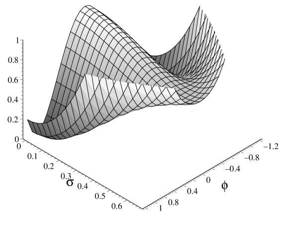
FIG. 2.: The two dimensional potential which may be used to describe the full non-linear field dynamics in a $\lambda\Phi^{4}$ new inflation phase transition in terms of effectively classical fields $\phi$ and $\sigma$. Axes are scaled such that the true minima of the potential occur at $\phi=\pm 1$.

We can also use the condition (47) to determine the value of the potential energy (46) during this phase. We find simply

$$V(\phi,\sigma)\to\frac{\mu^{4}}{\lambda}-\frac{\lambda}{12}\phi^{4}\;,$$ (49)

as is consistent with the effective mass for $\phi$. We see that the growth of fluctuations has produced an effective dynamics corresponding to a very flat potential for $\phi$ with a cosmological constant contribution to the energy density $\mu^{4}/\lambda$ which is $2/3$ of the value appearing in the original potential. We therefore arrive at a second stage of inflation with an expansion rate related to the original stage by a factor of $\sqrt{2/3}$.

We note, however, that there is a continued instability in $\phi$ with the consequence that eventually the condition

$$\phi^{2}\geq\phi_{s}^{2}=2\mu^{2}/\lambda\;,$$ (50)

is met and it becomes impossible to satisfy the sum rule (47). At this point, the second inflationary stage ends, the fluctuation field $\sigma$ decays away and the field $\phi$ evolves to its classical minimum.

B Natural Inflation

The natural inflation potential is derived from the vacuum manifold of a complex scalar field spontaneously broken at the Planck scale and with explicit symmetry breaking at the Grand Unified scale. It may be written in the form

$$V(\Phi)=\Lambda^{4}\left[1+\cos(\Phi/f)\right]\;,$$ (51)

where $\Lambda\sim M_{GUT}$ and $f\sim M_{Pl}$ are constants. Expansion of the cosine reveals that this potential is of the form (1) with $\mu^{2}\equiv\Lambda^{2}/f$ and $\lambda\equiv\Lambda^{4}/f^{4}$.

The reassembled equations of motion become:

$$\ddot{\phi}+3H\dot{\phi}-\frac{\Lambda^{4}}{f}\sin\left(\frac{\phi}{f}\right)\exp\left(-\frac{\sigma^{2}}{2f^{2}}\right) = 0\;,$$ (52)

$$\ddot{\sigma}+3H\dot{\sigma}-\frac{\Lambda^{4}}{f^{2}}\cos\left(\frac{\phi}{f}\right)\exp\left(-\frac{\sigma^{2}}{2f^{2}}\right)\sigma = 0\;,$$ (53)

$$\frac{\dot{a}^{2}}{a^{2}}=\frac{8\pi G_{N}}{3}\left[\frac{1}{2}\dot{\phi}^{2}+\frac{1}{2}\dot{\sigma}^{2}+\Lambda^{4}\left[1+\cos\left(\frac{\phi}{f}\right)\exp\left(-\frac{\phi^{2}}{2f^{2}}\right)\right]\right]\;.$$ (54)

We recognize these equations as those of a two homogeneous classical scalar fields with potential

$$V(\phi,\sigma)=\Lambda^{4}\left[1+\cos\left(\frac{\phi}{f}\right)\exp\left(-\frac{\sigma^{2}}{2f^{2}}\right)\right]\;.$$ (55)

We provide a plot of this two field potential in Fig. 3. As expected, for any integer $j$, we have degenerate maxima at $\phi=2j\pi f$, $\sigma=0$ and degenerate minima at $\phi=(2j+1)\pi f$, $\sigma=0$. The feature to notice, however, is that the potential quickly becomes very flat as $\sigma/f$ becomes greater than $1$.

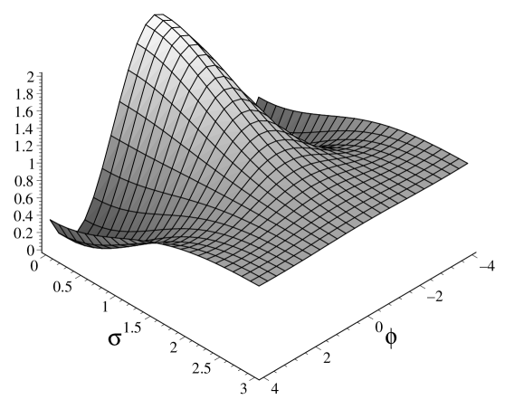
FIG. 3.: The two field classical potential for natural inflation. Axes are scaled such that the true minima of the potential occur at $\phi=(2j+1)\pi$.

Again, we concern ourselves with the fluctuation dominated regime. We find that the sum rule (41) results in the condition

$$\frac{\Lambda^{4}}{f^{2}}\cos\left(\frac{\phi}{f}\right)\exp\left(-\frac{\sigma^{2}}{2f^{2}}\right)\to 0\;,$$ (56)

which for $\phi<\pi f$ becomes satisfied as $\sigma$ grows large. The effective mass term for $\phi$ in (52) becomes exponentially suppressed as well, again indicating that the growth of fluctuations of the field results in a flattening of the potential. The potential itself clearly goes to the value $\Lambda^{4}$ which is precisely half of the value of the original cosmological constant contribution. This state of affairs will continue until $\phi\geq\phi_{s}=\pi f$, at which point the fluctuations represented by $\sigma$ become massive and begin to decay away.

As in the $\lambda\Phi^{4}$ model, we expect two stages of inflation, this time with the expansion rate of the second stage reduced from that of the first by the factor $\sqrt{2}$.

V Metric Perturbations

The possible link between inflationary expansion of the universe at Grand Unified energy scales and the observation of fluctuations in the Cosmic Microwave Background (CMB) temperature of order $10^{-5}$ is remarkable[32]. The fact that we are now in the process of observing the details of this temperature spectrum through a number of ground-, air-, and space-based experiments, presents an amazing opportunity for probing details of what the universe was like at times inaccessible through any other means[33].

In order to take full advantage of this opportunity, however, it is important that we are careful in connecting the observations to the theoretical models of the dynamical processes of the Early Universe which may have led to the CMB anisotropies. We have already presented a detailed analysis of the cosmological dynamics of scalar fields undergoing inflationary phase transitions. Here, we provide computations of the primordial spectra of density perturbations which arise from such phase transitions.

By computing the spectrum of scalar perturbations, we explicitly show that coherent effects due to large wavelength fluctuations of the inflaton field could have significant impact on observational features of the temperature spectrum of CMB anisotropies. Particular features of interest include scales on which there is deviation from a flat Harrison-Zel’dovich primordial power spectrum with power increasing as one moves to smaller scales. Such a spectrum, referred to as having a blue tilt (corresponding to a scalar tilt parameter $n_{s}>1$), was previously thought only to be possible in more complicated, multi-field models of inflation. Here, we find that it is indeed possible to produce such a spectrum on the length scales relevant to CMB anisotropy observations from the simplest of single field models.

Another significant feature of the spectra produced in phase transitions is the possible decrease in the amplitude of the primordial perturbations on the scales of interest relative to the predictions of an analysis assuming a classical evolution for the inflationary field. This may somewhat alleviate the fine tuning problem, although we find in practice that this effect is relatively minor, allowing perhaps a dimensionless quartic coupling for the field one or two orders of magnitude larger than previously thought. Since this coupling is typically thought to be restricted to be less than $10^{-14}$, we still require the inflationary models to be highly fine tuned.

A final feature of the spectra is their dependence on the precise initial state of the inflationary field in the region corresponding to today’s observational universe. It is found that a universe which began the inflationary phase in a strongly classical state will show none of the exotic features described here. This strongly contrasts with the case of initial states in which quantum fluctuations of the field are of the same order as the classical field value. In this latter case, the primordial spectrum may depend quite strongly on precisely how ‘quantum’ the particular initial state is.

We begin with a computation of the amplitude of scalar and tensor metric perturbations resulting from spinodal inflation. For the specific models discussed above, we provide details of the resulting power spectrum as a function of scale. We also include plots of the amplitude and tilt in the power spectrum as a function of the initial state of the scalar field for a choice of scale consistent with those observed by the Cosmic Background Explorer[32]. Finally, we provide examples of the $C_{l}$ temperature anisotropy spectra[19] that result from particularly interesting examples of spinodal inflationary effects to allow comparison with other theoretical plots of the $C_{l}$ spectrum and with the observed spectrum.

Note that in what follows, we use the normalizations of the scalar and tensor amplitudes of Ref. [18].

VI The Primordial Spectrum

Our starting point for the computation of primordial density perturbations is the expression for the average energy density (25). To compute the average fluctuation we define

$$\delta\varepsilon\equiv\left\langle\left(\delta T_{0}^{0}\right)^{2}\right\rangle^{1/2}\;,$$

where the variation of the energy density yields the expression

$$\left(\delta T_{0}^{0}\right)=\left(\dot{\phi}+\dot{\psi}\right)\dot{\psi}+\frac{1}{a^{2}}\left(\vec{\nabla}\psi\vec{\nabla}\right)\psi+\frac{\delta V(\phi+\psi)}{\delta\psi}\psi\;.$$ (57)

It is convenient to introduce the Fourier variable

$$\psi_{k}=\frac{k^{3/2}}{\sqrt{2}\pi}f_{k}\;,$$

defined such that

$$\langle\psi^{2}\rangle=\int\frac{dk}{k}|\psi_{k}|^{2}\;.$$

In Fourier space, we find the following expression for the average energy density fluctuation on a scale corresponding to a wavenumber $k$:

$$\left\langle\left(\delta T_{0}^{0}\right)\left(\delta T_{0}^{0}\right)\right\rangle_{k} = |\dot{\psi}_{k}|^{2}\left(\dot{\phi}^{2}+\langle\dot{\psi}^{2}\rangle\right)+\left(\psi_{k}\dot{\psi}_{k}^{*}+\dot{\psi}_{k}\psi_{k}^{*}\right)\left\langle\left((\dot{\phi}+\dot{\psi}\right)\frac{\delta V(\phi+\psi)}{\delta\psi}\right\rangle$$ (58)

$$+ |\psi_{k}|^{2}\left\langle\left(\frac{\delta V(\phi+\psi)}{\delta\psi}\right)^{2}\right\rangle\;,$$ (59)

where terms proportional to $1/a^{2}$ have been neglected. Normally during inflation, the third term on the right hand side of (59) dominates, which is equivalent to the statement that the usual slow roll conditions are satisfied during the evolution.

Using the above expression, the density contrast at first horizon crossing is

$$|\delta_{k=aH}|^{2}=\frac{1}{\rho^{2}}\left\langle\left(\delta T_{0}^{0}\right)\left(\delta T_{0}^{0}\right)\right\rangle\;.$$ (60)

Here, we note that we have used the important relation between the gauge invariant Bardeen variable representing the scalar metric perturbation and the energy density fluctuation at horizon crossing to allow us to write down this apparently simple expression. As the density perturbations are adiabatic (recall that there is only one scalar field with one set of fluctuations), the super-horizon evolution of the metric perturbation up to the second horizon crossing is specified by the conservation of a single parameter $\xi$ as defined in Ref. [18]. Following the procedure of Ref. [18], we arrive at the expression for the density contrast at mode re-entry in terms of the scaled mode functions $\psi_{k}$:

$$|\delta_{h}(k)|^{2}=\frac{\left[\left(\dot{\phi}^{2}+\langle\dot{\psi}^{2}\rangle\right)|\dot{\psi}_{k}|^{2}+\left\langle(\dot{\phi}+\dot{\psi})\frac{\delta V(\phi+\psi)}{\delta\psi}\right\rangle(\psi_{k}\dot{\psi}_{k}^{*}+\dot{\psi}_{k}\psi_{k}^{*})+\left\langle\left(\frac{\delta V(\phi+\psi)}{\delta\psi}\right)^{2}\right\rangle|\psi_{k}|^{2}\right]}{25\left(\dot{\phi}^{2}+\langle\dot{\psi}^{2}\rangle\right)^{2}}\;,$$ (61)

where each quantity is evaluated at the time when the corresponding mode first crosses the horizon, i.e. when $k=aH$.

In what follows, we will assume that the third term in (59) dominates over the first two terms, as this is an excellent approximation in the models in which we are interested. Eq. (61) becomes simply:

$$|\delta_{h}(k)|^{2}\simeq\frac{|\psi_{k}|^{2}\left\langle\left(\frac{\delta V(\phi+\psi)}{\delta\psi}\right)^{2}\right\rangle}{25\left(\dot{\phi}^{2}+\langle\dot{\psi}^{2}\rangle\right)^{2}}\;.$$ (62)

This can be simplified further by recognizing that at first horizon crossing the quantity $|\psi_{k}|^{2}$ is given approximately by $(H/2\pi)^{2}$[34]. This may be seen directly from the asymptotic solutions of the mode functions for large momenta. As the expansion is rapid, these asymptotic solutions remain approximately valid all the way to $k\sim aH$. Combining this with the (semi-classical) Friedmann equation and using the inflationary condition $\langle V\rangle\gg\dot{\phi}^{2}+\langle\dot{\psi}^{2}\rangle$, we reach the result

$$|\delta_{h}(k)|^{2}\simeq\frac{2}{75\pi}\frac{\langle V\rangle\langle V_{,\psi}^{2}\rangle}{M_{Pl}^{2}(\dot{\phi}^{2}+\langle\dot{\psi}^{2}\rangle)^{2}}\;.$$ (63)

If we were to make the further assumption that the fluctuations are always small with $\psi\ll\phi$ and $\dot{\psi}\ll\dot{\phi}$, then we would arrive at the standard slow roll expression for the density contrast:

$$|\delta_{h}(k)|=\sqrt{6\pi}\frac{8}{5}\frac{V^{3/2}}{|V^{\prime}|M_{Pl}^{3}}\;.$$ (64)

We will continue, however, with the more general form (63).

The computation of the tilt parameter $n_{s}-1$ is straightforward, given (63). We define

$$n_{s}-1\equiv\left.\frac{d(\ln|\delta_{h}(k)|)}{d\ln(k)}\right|_{k=aH}\;.$$ (65)

As is common practice, we could rewrite this expression in terms of partial derivatives of the field variables. However, since we have dependence both upon $\phi$ and the fluctuations $\psi$, such a procedure results in a complicated expression which is not particularly instructive. We will therefore satisfy ourselves with (65), which is used directly to compute the tilt parameter in the numerical examples.

A $\lambda\Phi^{4}$ Spinodal Inflation

Using (63), we now compute the expression for the primordial spectrum of scalar metric perturbations specific to the $\lambda\Phi^{4}$ model of spinodal inflation. In terms of the reassembled variables $\phi$ and $\sigma$, the result is:

$$|\delta_{h}(k)| = \sqrt{\frac{2}{75\pi}}\frac{1}{M_{Pl}\left(\dot{\phi}^{2}+\dot{\sigma}^{2}\right)}\left[\frac{3\mu^{4}}{2\lambda}-\frac{1}{2}\mu^{2}\left(\phi^{2}+\sigma^{2}\right)+\frac{\lambda}{24}\left(\phi^{4}+6\phi^{2}\sigma^{2}+3\sigma^{4}\right)\right]^{1/2}$$ (66)

$$\times \left[\mu^{4}\left(\phi^{2}+\sigma^{2}\right)-\frac{\lambda\mu^{2}}{3}\left(\phi^{4}+6\phi^{2}\sigma^{2}+3\sigma^{4}\right)\right.$$ (68)

$$\left.+\frac{\lambda^{2}}{36}\left(\phi^{6}+15\phi^{4}\sigma^{2}+45\phi^{2}\sigma^{4}+15\sigma^{6}\right)\right]^{1/2}\;.$$

Again, we point out that all expressions are to be evaluated when the given scale $k$ crosses the horizon.

B Natural Inflation

For natural inflation, the relevant expression is:

$$|\delta_{h}(k)|=\frac{\Lambda^{6}}{\sqrt{75\pi}M_{Pl}f\left(\dot{\phi}^{2}+\dot{\sigma}^{2}\right)}\left(1-\cos\left(2\phi/f\right)e^{-2\sigma^{2}/f^{2}}\right)^{1/2}\left(1+\cos\left(\phi/f\right)e^{-\sigma^{2}/2f^{2}}\right)^{1/2}\;.$$ (69)

C Gravitational Wave Perturbations

It is also of interest to examine the spectrum of gravitational wave perturbations resulting from spinodal inflation. As such perturbations do not directly interact with the inflaton field, they may be related directly to the expansion rate during any inflationary stages. During such regimes, the amplitude of gravitational waves is simply[18]:

$$|\delta_{g}(k)|=\frac{2}{\sqrt{3\pi}}\frac{H_{k}}{M_{Pl}}\;,$$ (70)

where $H_{k}$ is the value of the expansion rate when the scale $k$ first crosses the horizon, $k=aH_{k}$.

As we have discussed, spinodal inflation may involve two distinct inflationary stages. The relevant amplitude of the gravitational waves is therefore typically determined by which stage is in effect 60–50 $e$-folds before the end of inflation, when the relevant length scales exit the horizon. However, the transition period between inflationary stages may also be relevant.

The spectrum in the transition period depends upon the details of the transition, but clearly must smoothly interpolate between the two major regimes. The important factor is whether the characteristic accelerated expansion continues to hold throughout the transition or if the transition includes a short period of deceleration. In the former case, the transition is smooth and straightforward, following Eq.(70) throughout, while in the latter case, the amplitude of the modes crossing the horizon during the transition has an oscillatory nature[18].

As we will see, the former, smooth transition without any oscillation of the gravitational wave amplitude is typical of spinodal inflation, with the result that the spectrum may have at most a single feature indicative of the transition from the initial inflationary phase to the spinodal phase.

D Notes on metric perturbations

It is worth taking a moment to examine the significance of the expressions for the amplitudes of the metric perturbations in some detail. The first feature to notice is that the scalar amplitude depends directly upon both the average field value $\phi$ and the typical fluctuation represented by $\sigma$. As we have seen, the end of inflation depends upon the evolution of $\phi$, occurring when $\phi$ reaches the spinodal value $\phi_{s}$. When the influence of the field fluctuations are neglected, the value of $\phi$ $60$ $e$-folds before the end of inflation, $\phi_{60}$, which we will take to be the largest scale measured by COBE, is a well defined quantity and corresponds to a well defined scalar amplitude $|\delta_{60}|$ independent of the initial conditions.

However, we see here that the dynamics of the field fluctuations $\sigma$ may influence the evolution of $\phi$. The net result is that the precise values of $\phi_{60}$, $\sigma_{60}$, and therefore $|\delta_{60}|$ occuring when the relevant mode crosses the horizon does generally depend upon the initial conditions for the inflaton.

This leads to an extremely important result: The spectrum of primordial metric perturbations resulting from a given model of inflation depends upon the initial state of the inflaton field.

A second significant feature coming as a result of these more general expressions for the perturbation amplitude is that $|\delta_{h}(k)|$ is not necessarily a monotonically increasing function of length scale. In contrast to the case in which the influence of the field fluctuations are neglected, there may be periods of time during which $|\delta_{h}(k)|$ increases as ever shorter length scales cross the horizon.

This leads to a result previously thought to be impossible in such simple, single field inflationary models: Inflation may result in a blue spectral tilt in the primordial spectrum of scalar perturbations.

E The $C_{l}$ Spectrum

As a final note in this section, we recall that none of the parameters of the primordial spectrum written down to this point are directly observable. Rather, this primordial spectrum becomes processed by the evolution of the late time universe, after corresponding length scales have re-entered the particle horizon. The most important set of observable parameters is the $C_{l}$ spectrum of the Cosmic Microwave Background map of temperature variations.

Standard techniques of computing the $C_{l}$’s from the primordial parameters assume a scale independent tilt $n_{s}$, which does not generally apply here. It is, of course, possible to compute the $C_{l}$ spectrum for a more general primordial spectrum, but to do so is far beyond the scope of the present work. We therefore use a standard approximation which relates the tilted spectrum $C_{l}^{(tilt)}$ to the tilted scalar perturbation amplitude $|\delta_{h}(k)^{tilt}|$ evaluated on the scale $k=lH_{*}/2$ where $H_{*}$ is the inverse Hubble radius today relative to the respective quantities where a flat spectrum ($n_{s}=1$) is assumed[35]:

$$C_{l}^{(tilt)}=C_{l}^{(flat)}\frac{|\delta_{h}(k=lH_{*}/2)^{tilt}|^{2}}{|\delta_{h}(k=lH_{*}/2)^{flat}|^{2}}\;.$$ (71)

Assuming the spectrum $C_{l}^{(flat)}$ used here is properly COBE normalized, we require that the flat and tilted primordial amplitude match for the low $l$ scales corresponding to COBE.

This will allow us to present an approximate plot of the $C_{l}$ spectrum resulting from spinodal effects which may be compared to standard $C_{l}$ spectra.

VII Concrete examples and results

We now put all the pieces of the previous sections together in numerical simulations of the full dynamical equations of motion of the spinodal system. A note is in order regarding these simulations. In certain cases it was impractical to run numerical simulations using the full field theory equations of motion. These include plots showing quantities as a function of the initial condition for $\phi$ as well as the plot of the scalar tilt as a function of the initial Hubble parameter. In these cases, we turned to the classical 2-field models described above, using the approximate initial condition $\sigma(t_{0})=H_{0}/2\pi$. All such figures specify in the caption that they result from the classical models. All other figures were produced from full field theory simulations.

A New Inflation

We begin with the $\lambda\Phi^{4}$ system, which we first examined in this context in Ref. [17]. We show the dynamics of the mean field $\phi$, the fluctuation $\langle\psi^{2}\rangle^{1/2}$, each of which is scaled by the factor $f\equiv\mu\sqrt{6/\lambda}$, and the expansion rate $H$ for each of three examples, corresponding to (a) $\phi(t_{0})\gg H_{0}/2\pi$, (b) $\phi(t_{0})\simeq H_{0}/2\pi$, and (c) $\phi(t_{0})\ll H_{0}/2\pi$.

In the first of these, (a), shown in Fig. 4, the evolution proceeds exactly as would be expected from a purely classical analysis of the dynamics. The two-point fluctuation $\langle\psi^{2}\rangle$ remains small and does not have a noticeable effect on the evolution of $\phi$, which in turn simply follows the contour of the tree-level effective potential $V(\phi)$. As $\langle\psi^{2}\rangle$ remains small, the expressions for the amplitude of primordial metric perturbations (61) reduces to the usual slow roll expression (64) and we arrive at the standard results for $|\delta_{h}(k)|$, $n_{s}-1$, and $|\delta_{g}|$. These quantities are depicted in Fig. 5 as a function of $N$, the number of $e$-folds before the end of inflation at which the corresponding length scale crosses the horizon.

FIG. 4.: The mean field $\phi(t)/f$, the fluctuation $<\psi^{2}(t)>^{1/2}/f$, and the Hubble parameter $H(t)/\mu$ vs. $t$ for the $\lambda\Phi^{4}$ model with $\phi(t_{0})=5.0H_{0}/2\pi$, $\dot{\phi}(t_{0})=0$, $H_{0}=2\mu$, $\lambda/8\pi^{2}=10^{-16}$, and $f\equiv\mu\sqrt{6/\lambda}$.

FIG. 5.: The scalar amplitude $\delta_{h}$, the scalar tilt $n_{s}-1$, and the tensor amplitude $\delta_{g}$ vs. $N$ corresponding to the evolution of Fig. 4.

Example (b), Fig. 6, is an intermediate example for which the fluctuation becomes large for a short time, inducing a spinodal phase during the period of evolution for which the length scales of relevance to CMB observations cross the horizon. This example is of further importance because it depicts the case in which the initial classical value of the inflaton field is of the same order as its initial vacuum fluctuations. As is clearly shown, the growth of the two-point fluctuation has a significant influence on the evolution of the mean field $\phi$, resulting as well in a modified behavior for the expansion.

FIG. 6.: The mean field $\phi(t)/f$, the fluctuation $<\psi^{2}(t)>^{1/2}/f$, and the Hubble parameter $H(t)/\mu$ vs. $t$ for the $\lambda\Phi^{4}$ model with $\phi(t_{0})=0.4H_{0}/2\pi$, $\dot{\phi}(t_{0})=0$, $H_{0}=2\mu$, $\lambda/8\pi^{2}=10^{-16}$, and $f\equiv\mu\sqrt{6/\lambda}$.

The result for the metric perturbations are provided in Fig. 7, where we see some remarkable features. First, we notice that the amplitude of $|\delta_{h}(k)|$ is reduced and that its shape is significantly changed by the spinodal dynamics. The significance of the shape is further emphasized by the scalar tilt $n_{s}-1$. Here, we see that for some scales of observational relevance between $60$ and $50$ $e$-folds before the end of inflation, the scalar tilt parameter $n_{s}-1$ is positive. This corresponds to a blue tilt in the power spectrum and was, until now, considered to be unattainable in inflation models consisting of only a single scalar field. Finally, the tensor amplitude clearly follows the behavior of the expansion rate $H$ as expected.

FIG. 7.: The scalar amplitude $\delta_{h}$, the scalar tilt $n_{s}-1$, and the tensor amplitude $\delta_{g}$ vs. $N$ corresponding to the evolution of Fig. 6.

To show why this is the case, we plot in Fig. 8 the equation of state $w\equiv p/\rho$ as a function of time. We see that in the transition region between the initial and spinodal phases of inflation, there is little departure from the de Sitter equation of state $p=-\rho$ and that, in particular, $p<-\rho/3$ through to the end of the second inflationary stage. This means that the condition for accelerated expansion $\ddot{a}>0$ is satisfied the whole time, resulting in the simple behavior of the tensor amplitude.

FIG. 8.: The equation of state $w(t)\equiv p(t)/\varepsilon(t)$ vs. $t$ for the parameters corresponding to the evolution of Fig. 6. The expanded region shows the transition between the initial and spinodal phases of inflation.

Case (c), Fig. 9 shows the other extreme case when the initial classical value of the field is significantly smaller than the effective quantum fluctuation. Here, $\langle\psi^{2}\rangle$ reaches the spinodal while $\phi$ remains small, resulting in a very long spinodal phase in which the mean field $\phi$ evolves slowly along the spinodal line. The results for the metric parameters are provided in Fig. 10.

FIG. 9.: The mean field $\phi(t)/f$, the fluctuation $<\psi^{2}(t)>^{1/2}/f$, and the Hubble parameter $H(t)/\mu$ vs. $t$ for the $\lambda\Phi^{4}$ model with $\phi(t_{0})=0.05H_{0}/2\pi$, $\dot{\phi}(t_{0})=0$, $H_{0}=2\mu$, $\lambda/8\pi^{2}=10^{-16}$, and $f\equiv\mu\sqrt{6/\lambda}$.

FIG. 10.: The scalar amplitude $\delta_{h}$, the scalar tilt $n_{s}-1$, and the tensor amplitude $\delta_{g}$ vs. $N$ corresponding to the evolution of Fig. 9.

To add completeness to this picture, it is useful to plot the scalar amplitude and tilt as a function of the log of the initial value $\phi(t_{0})$ over the range of the differing regimes. This is done for the particular scale crossing the horizon $60$ $e$-folds before the end of inflation (Fig. 11). This figure provides a nice summary of our primary results.

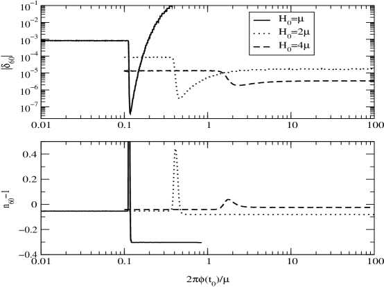
FIG. 11.: The scalar amplitude $\delta_{60}$ and the scalar tilt $n_{60}-1$ corresponding to the scale crossing the horizon $60$ $e$-folds before the end of inflation vs. $2\pi\phi(t_{0})/\mu$ for $\lambda\Phi^{4}$ new inflation using the classical two field model with $\dot{\phi}(t_{0})=0$, $\lambda/8\pi^{2}=10^{-16}$ and several values of $H_{0}$.

In the classical regime $\phi(t_{0})\gg H_{0}/2\pi$, the results are independent of initial conditions, but as $\phi(t_{0})$ becomes of order $H_{0}/2\pi$ there is a distinct transition regime in which the amplitude drops by up to a couple of orders of magnitude (possibly alleviating the fine tuning problem of inflation to a minor degree), while there is a spike for which the tilt becomes positive. While this region appears rather restricted in the parameter space of initial values for $\phi$, we remind the reader that we plot here on a log scale the ratio of $\phi(t_{0})$ to $\mu/2\pi$ so that the region in question effectively covers the entire range for which $\phi(t_{0})$ and $H_{0}/2\pi$ are of the same order of magnitude.

Finally, we see distinct regions for which there is a long spinodal phase. In this case, $\langle\psi^{2}\rangle$ has a significant effect long before the relevant scales cross the horizon. The mean field evolves slowly along the spinodal line to the spinodal point. As the sum rule (41) is in place during this phase, the evolution of $\phi$ in the latter stages is always the same, and we therefore expect that $|\delta_{60}|$ and $n_{60}-1$ become constant throughout this regime, as is indeed the case.

It is worth mentioning how these results depend upon the other parameters of the model, such as the magnitude of the quartic coupling $\lambda$ and the ratio of the initial expansion rate to the mass scale $H_{0}/\mu$.

Increasing the value of $\lambda$ while keeping $H_{0}/\mu$ fixed only acts to modify the value of the vacuum expectation value and the spinodal point to be smaller as both of these quantities are proportional to $1/\sqrt{\lambda}$. This simply reduces the amount of time the fields evolve, but does not change any of the features described above, with the exception that the scalar amplitude $|\delta_{h}(k)|$ scales, as usual, as $\sqrt{\lambda}$.

Modification of the ratio $H_{0}/\mu$ (keeping $\lambda$ fixed), on the other hand has a more complex influence on the behavior. The results for the scalar amplitude and tilt as a function of initial conditions for three values of $H_{0}/\mu$ are shown in Figs. 11. Here, we see that increasing the parameter has the effect of reducing the amplitudes of the features in the transition region.

Note that in the case of $H_{0}/\mu=1$ the approximations we have used to compute the metric perturbation spectrum break down in the transition region, where we see that the scalar tilt spikes to a very large value, and therefore this computation is unreliable for that small range of initial conditions. However, as long as the transition period does not occur within the last $60$ $e$-folds of inflation, and in particular for the spinodal region for $\phi(t_{0})\ll H_{0}/2\pi$, the slow roll conditions are satisfied throughout the relevant period of evolution such that the portions of this plot away from the transition region are reliable.

Finally, we mention a somewhat unexpected feature of the results for the spinodal regime with small initial $\phi(t_{0})$. In Fig. 12, we plot the scalar tilt parameter $n_{s}-1$ as a function of the value of the initial Hubble parameter $H_{0}/\mu$ and compare it to the result in the classical regime for which $n_{s}-1=\mu^{2}/3H_{0}^{2}$. The result is remarkable. Over a large range of initial expansion rates, there is very little change in the value of the scalar tilt. It seems that the tilt due to a long spinodal phase of inflation is relatively independent of the parameters of the model, with an empirical prediction over the range of tested parameters of $0.94<n_{s}<0.98$. While extension to even larger values of $H_{0}/\mu$ may bring the upper limit toward $1.0$, it seems likely that the lower limit will remain solid. The consequence is that a future measurement which restricts the tilt to $n_{s}<0.94$ would seem to rule out a spinodal phase of inflation.

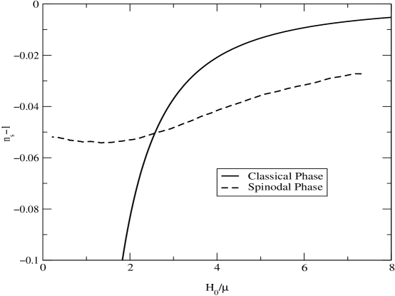
FIG. 12.: The scalar tilt $n_{60}-1$ corresponding to the scale crossing the horizon $60$ $e$-folds before the end of inflation vs. $H_{0}/\mu$ for $\lambda\Phi^{4}$ new inflation using the classical two field model and spinodal initial conditions, ${\phi}(t_{0})\ll H_{0}/2\pi$.

B natural inflation

Due to its popularity, we examine one other spinodal inflation model in detail: natural inflation. The qualitative behavior is in many ways quite similar to that of the $\lambda\Phi^{4}$ model described above, so we will focus on the distinguishing features. The primary difference occurs during the spinodal phase. In the $\lambda\Phi^{4}$ model, the spinodal condition of Eq. (41) simply results in the lowest order contribution to the effective mass squared of the true zero mode $\phi$ being of order $-\lambda\phi^{2}$, thus slowing the evolution of $\phi$. In natural inflation, however, the spinodal condition for natural inflation yields an effective mass which is exponentially suppressed by the growth of the fluctuations. Hence, the evolution of the zero mode can come to practically a standstill. The net result is that the spinodal phase in natural inflation models is significantly longer than a corresponding $\lambda\Phi^{4}$ model.

We provide results for two examples corresponding to the intermediate case with $\phi(t_{0})\simeq H_{0}/2\pi$ shown in Figs. 13 and 14 and the fully fluctuation dominated case of $\phi(t_{0})\ll H_{0}/2\pi$ as depicted in Figs. 15 and 16. We see the same features that appeared in the previous model, with the obvious difference that the spinodal phase of Fig. 15 is extremely long even for $\phi(t_{0})$ not much smaller than $H_{0}/2\pi$.

FIG. 13.: The mean field $\phi(t)/f$, the fluctuation $<\psi^{2}(t)>^{1/2}/f$, and the Hubble parameter $H(t)/\mu$ vs. $t$ for the natural inflation model with $\phi(t_{0})=H_{0}/2\pi$, $\dot{\phi}(t_{0})=0$, $H_{0}=2\mu$, and $\Lambda^{4}/4\pi^{2}f^{4}=10^{-16}$.

FIG. 14.: The scalar amplitude $\delta_{h}$, the scalar tilt $n_{s}-1$, and the tensor amplitude $\delta_{g}$ vs. $N$ corresponding to the evolution of Fig. 13.

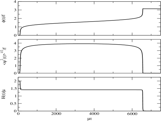
FIG. 15.: The mean field $\phi(t)/f$, the fluctuation $<\psi^{2}(t)>^{1/2}/f$, and the Hubble parameter $H(t)/\mu$ vs. $t$ for the natural inflation model with $\phi(t_{0})=0.5H_{0}/2\pi$, $\dot{\phi}(t_{0})=0$, $H_{0}=2\mu$, and $\Lambda^{4}/4\pi^{2}f^{4}=10^{-16}$.

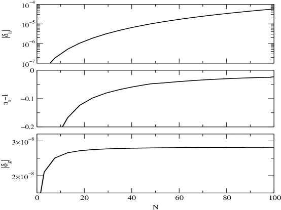
FIG. 16.: The scalar amplitude $\delta_{h}$, the scalar tilt $n_{s}-1$, and the tensor amplitude $\delta_{g}$ vs. $N$ corresponding to the evolution of Fig. 15.

It is worth examining this point further by plotting the number of $e$-folds of inflation as a function of the initial condition on $\phi$. This is shown in Fig.17 where we see a dramatic dependence which contrasts very sharply with the logarithmic dependence of the same quantity on initial conditions in the classical regime.

FIG. 17.: The total number of $e$-folds of inflation $N$ vs. $2\pi\phi(t_{0})/H_{0}$ for natural inflation using the classical two field model with $\dot{\phi}(t_{0})=0$, $\Lambda^{4}/4\pi^{2}f^{4}=10^{-16}$ and $H_{0}=2\Lambda^{2}/f$.

Once again, it is enlightening to examine the dependence of the quantities $|\delta_{60}|$ and $n_{60}-1$ as a function of the initial state. These are depicted in Figs. 18 where we see again the clear transition regime around $\phi(t_{0})\sim H_{0}/2\pi$ separating the classical and fluctuation dominated regimes.

FIG. 18.: The scalar amplitude $\delta_{60}$ and the scalar tilt $n_{60}-1$ vs. $2\pi\phi(t_{0})/H_{0}$ for natural inflation using the classical two field model with $\dot{\phi}(t_{0})=0$, $\Lambda^{4}/4\pi^{2}f^{4}=10^{-16}$ and $H_{0}=2\Lambda^{2}/f$.

C Example $C_{l}$ Spectrum

Finally, we present an example $C_{l}$ spectrum resulting from spinodal inflation, shown in Fig. 19. We plot the tilted $C_{l}$ spectrum corresponding to the natural inflation case of Fig. 13 as well as a standard flat $C_{l}$ spectrum for comparison. The ‘flat’ spectrum was produced using the program CMBFAST version 2.4.1[36] using the defaults of a standard Cold Dark Matter cosmology with a tiltless adiabatic power spectrum $n_{s}=1$, while the ‘curved’ spectrum was reproduced from the flat one using the approximate relation (71).

The primary feature of interest is that while the spinodal inflation spectrum is shifted downward for the modes $100<l<1000$, the spectrum approaches its flat counterpart for high $l$. This is indicative of the shift of the spectrum from red to blue over the range of observable scales.

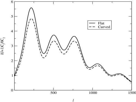
FIG. 19.: The standard CDM $C_{l}$ spectrum of temperature anisotropies vs. $l$ for a flat $n_{s}=1$ spectrum and the curved spectrum corresponding to the evolution of Fig. 13.

VIII Conclusions

Whether one studies QCD, ferromagnetism, or ordinary gases, non-linear, long wavelength effects are seen to have a dramatic impact on the properties of the physical system. Without close contact between the observation and theory of these systems, there is good reason to doubt whether the respective phenomena of confinement, ferromagnetism, or the liquid-gas phase transition would be as well understood as they are today. But that is precisely the challenge before us if we wish to understand the dynamics of phase transitions in the very early stages of the universe.

If we expect to be able to proceed, then it will be necessary to return to those systems that we believe we understand, say in condensed matter physics, and examine the techniques, approximations, and concepts which have led to consistent and accurate theoretical descriptions. Looking in any statistical physics text we immediately notice that there are a few general concepts and techniques which have been found to be particularly rewarding for a variety of different systems.

One of these is mean field theory, where complex details of a system are replaced by simple averages. It is in many ways a very naive approach and often provides quantitative results which are only roughly correct. But the real power of mean field theory lies not only in its quantitative predictions, rather in the qualitative pictures it paints, allowing us, for example, to explain the liquid-gas phase transition in terms of a system as simple as that given by the van der Waals equation of state.

Another powerful concept is the convexity of the thermodynamical free energy function for any equilibrium system and the simple rules for writing down such a function provided by the Maxwell construction. The story being told by these concepts is that theoretical energy curves with concave portions describe ‘unphysical’ states, and that the dynamics of the corresponding system will act to transform any such state into a physical state described by a purely convex energy function.

This report is an attempt to understand the system of an inflationary phase transition in the context of these powerful concepts. The initial state is unphysical, described by a concave effective potential, the analog of the equilibrium free energy, with quanta corresponding to imaginary mass states. Such a system must decay into physical states, which we see from the exponential growth of long wavelength fluctuations. This decay continues until a non-perturbative state is reached for which the corresponding quanta are physical with a strictly real or zero mass.

There are two possible ways to reach such a state. The first is simply to provide a significant bias to the state such that the mean value of the field (i.e. the order parameter) reaches its true vacuum value where the field quanta are well defined.

The second way, appropriate for systems with small order parameter, is to allow the system to phase separate into domains for which the field has either positive or negative value. Rather than the order parameter moving along the potential energy diagram (see Fig. 1), the field drops down into the center of the diagram to the spinodal line. At the spinodal line, the field quanta are massless and physical, and this state of affairs may be relatively long lasting, ending only when one phase becomes so much more prevalent than the other that the system may relax into a definite vacuum state throughout the system.

We therefore have arrived at a consistent physical picture of inflationary phase transitions based upon mean field theory. Already, at this naive level, we have seen new phenomena which impact not only the evolution of the inflaton field but also have important implications for the interpretation of recent and soon to come observational data.

As a final note, we emphasize that the techniques used here are really only a first – or, rather, a second – approximation to a very complicated system of interaction between an unstable scalar field and gravity at very high energies. There are a number of possible avenues which might be taken to improve upon these results for the dynamics and, in particular, for the predictions of observational quantities.

One direction is to move beyond mean field theory. Gravitationally, this means doing something more sophisticated than semi-classical gravity. There has been recent work in this regard within the context of perturbation theory up to two loop order[37], and interest in this area has grown somewhat due to the possibility of new phenomena in the context of preheating[38]. However, the non-perturbative dynamics of the scalar field studied here corresponds to non-perturbative departures of the gravitational dynamics from that of a purely classical background field so that techniques based upon perturbative expansions are of little help.

In terms of the scalar field dynamics, one possible avenue that has received attention is the $1/N$ expansion of the $O(N)$ vector model, which includes contributions beyond mean field theory at next to leading order (this approximation is also promising as it might be consistently implemented for gravity as well)[39]. Another alternative approach is to use variational methods to compute the dynamics of the system[40], a technique which might also be combined with the $1/N$ expansion. However, significant hurdles remain before either of these techniques will be implementable for interesting field theory problems.

The primary alternative to these semi-analytic approaches is to look to lattice simulations. As the interesting phenomena occur out of equilibrium, fully quantum simulations are ruled out and our only alternative is to examine real time simulations of a classical scalar coupled to classical gravity. This approach has led, in particular, to improvements in our understanding of preheating dynamics[10, 41]. However, extending these methods to interesting problems in inflationary dynamics will be a challenge requiring a fully general relativistic lattice coupled to the inflaton field, a way to properly deal with an exponentially changing scale, and a method of introducing classical fluctuations consistent with the classicalization of quantum, sub-horizon field modes as they cross the horizon.

The challenges are great, but we should be encouraged both by the improved physical picture presented here and by the incredible fact that inflationary theory is on the verge of becoming an observational science.

- [1] For reviews on topological defects in early universe cosmology, see: A. Vilenkin and E. P.S. Shellard, Cosmic Strings and other Topological Defects, Cambridge University Press, (1994); M. B. Hindmarsh and T. W. B. Kibble, Rep. Prog. Phys. 58, 477 (1995).
- [2] A. D. Dolgov and A. D. Linde, Phys. Lett. B116, 329 (1982); L. F. Abbott, E. Farhi and M. Wise, Phys. Lett. B117, 29 (1982); D. Boyanovsky, H. J. de Vega, R. Holman, D.-S. Lee and A. Singh, Phys. Rev. D51, 4419 (1995).
- [3] A. H. Guth, Phys. Rev. D23, 347 (1981).
- [4] J. Traschen and R. Brandenberger, Phys Rev D42, 2491 (1990); Y. Shtanov, J. Traschen and R. Brandenberger, Phys. Rev. D51, 5438 (1995); L. Kofman, A. Linde and A. Starobinsky, Phys. Rev. Lett. 73, 3195 (1994) and 76, 1011 (1996).
- [5] L. Dolan and R. Jackiw, Phys. Rev. D9, 3320 (1974); G. F. Mazenko, W. G. Unruh and R. M. Wald, Phys. Rev. D31, 273 (1985); G. F. Mazenko, Phys. Rev. Lett. 54, 2163 (1985); D. Boyanovsky and H. J.. de Vega, Phys. Rev. D47, 2343 (1993).
- [6] A. Linde, Particle Physics and Inflationary Cosmology, (Harwood Academic Publishers, Switzerland, 1990); E. W. Kolb and M. S. Turner, The Early Universe, Addison Wesley, Redwood City, (1990).
- [7] A. A. Starobinsky, in Fundamental Interactions (MGPI Press, Moscow, 1983); in Current Topics in Field Theory, Quantum Gravity, and Strings edited by H. J. de Vega and N. Sanchez (Springer, New York, 1986).
- [8] S. Habib, Phys. Rev. D46, 2408 (1992); A. Matacz, Phys. Rev. 55, 1860 (1997).
- [9] D. Polarski and A. A. Starobinsky, Class. Quant. Grav. 13, 377 (1996); J. Lesgourgues, D. Polarski and A. A. Starobinsky, Nucl. Phys. B497, 479 (1997) and references therein.
- [10] S. Yu. Khlebnikov and I.I. Tkachev, Phys. Rev. Lett. 77, 219 (1996); S. Yu. Khlebnikov and I.I. Tkachev, Phys. Lett. B390, 80 (1997).
- [11] J. W. Cahn, Trans. Metall. Soc. AIME 242, 166 (1968); J. E. Hilliard, in Phase Transformations, edited by H. I. Aronson (American Society for Metals, Metals Park, Ohio, 1970).
- [12] A. D. Linde, Phys. Lett. B108, 389 (1982); A. Albrecht and P .J. Steinhardt, Phys. Rev. Lett. 48, 1220 (1982); A. Vilenkin, Nucl. Phys. B226, 527 (1983); P. J. Steinhardt and M. S. Turner, Phys. Rev. D29 2162 (1984).
- [13] K. Freese, J. A. Frieman and A. V. Olinto, Phys. Rev. Lett. 65, 3233 (1990).
- [14] A. D. Linde, Phys. Lett. B259, 38 (1991); E. J. Copeland, E. W. Kolb, A. R. Liddle and J. E. Lidsey, Phys. Rev. D48, 2529 (1993).
- [15] D. Booyanovsky, H. J. De Vega, R. Holman, “Non-Equilibrium Phase Transitions in Condensed Matter and Cosmology: Spinodal Decomposition, Condensates and Defects”, Los Alamos Preprint Archive hep-ph/9903534 (1999).
- [16] D. Boyanovsky, D. Cormier, H. J. de Vega, R. Holman and P. Kumar Phys. Rev. D57, 2166 (1998).
- [17] D. Cormier and R. Holman, Phys. Rev. D60, 41301 (1999).
- [18] V. F. Mukhanov, H. A. Feldman and R. H. Brandenberger, Phys. Rep. 215, 205 (1992).
- [19] P. J. E. Peebles, Astrophys. J. Lett. 263, L1 (1982).
- [20] A. Guth and S-Y. Pi, Phys. Rev. D32, 1899 (1985).
- [21] P. A. M. Dirac, Proc. Cambridge Philos. Soc. 26, 376 (1930).
- [22] See, for example, A. L. Fetter and J. D. Walecka, Quantum Theory of Many-Particle Systems, McGraw-Hill, New York (1971); T. Kinoshita and Y. Nambu, Phys. Rev. 94, 598 (1954); S. J. Chang, Phys. Rev. D12, 1071 (1975).
- [23] S. Weinberg, Phys. Rev. D9, 3357 (1974).
- [24] J. Schwinger, J. Math. Phys. 2, 407 (1961); P. M. Bakshi and K. T. Mahanthappa, J. Math. Phys. 4, 1 (1963); ibid, 12; L. V. Keldysh, Sov. Phys. JETP 20, 1018 (1965); A. Niemi and G. Semenoff, Ann. of Phys. (N.Y.) 152, 105 (1984); Nucl. Phys. B [FS10], 181 (1984); E. Calzetta, Ann. of Phys. (N.Y.) 190, 32 (1989); R. D. Jordan, Phys. Rev. D33, 444 (1986); N. P. Landsman and C. G. van Weert, Phys. Rep. 145, 141 (1987); R. L. Kobes and K. L. Kowalski, Phys. Rev. D34, 513 (1986); R. L. Kobes, G. W. Semenoff and N. Weiss, Z. Phys. C29, 371 (1985).
- [25] D. Boyanovsky, D. Cormier, H. J. de Vega, R. Holman, A. Singh, M. Srednicki, Phys. Rev. D56, 1939 (1997);
- [26] J. Baacke, K. Heitmann and C. Pätzold, Phys. Rev. D57, 6398 (1998).
- [27] S. A. Ramsey and B. L. Hu, Phys. Rev. D56, 661 (1997).
- [28] C. Molina-Paris, P. R. Anderson and S. A. Ramsey, “One-loop Theory in Robertson-Walker Spacetimes: Adiabatic Regularization and Analytic Approximation”, Los Alamos Preprint Archive gr-qc/9908037 (1999).
- [29] P. R. Anderson, Phys. Rev. D32, 1302 (1985).
- [30] J. Baacke, K. Heitmann and C. Pätzold, Phys. Rev. D55, 2320 (1997); Phys. Rev. D56, 6556 (1997).
- [31] C. Destri and E. Manfredini, “Out-of-Equilibrium Dynamics of QFT in Finite Volume”, Los Alamos Preprint Archive hep-ph/9906554 (1999).
- [32] C. L. Bennett et al., Astrophys. J. 464, L1 (1996).
- [33] M. Kamionkowski and A. Kosowsky, “The Cosmic Microwave Background and Particle Physics”, Los Alamos Preprint Archive astro-ph/9904108, to appear in Annual Reviews of Nuclear and Particle Science (1999).
- [34] A. Vilenkin and L. H. Ford, Phys. Rev. D25, 1231 (1982); A. D. Linde, Phys. Lett. B116, 335 (1982); A. A. Starobinsky, Phys. Lett. B117, 175 (1982).
- [35] A. R. Liddle and D. H. Lyth, Phys. Rep. 231, 1 (1993).
- [36] U. Seljak and M. Zaldarriaga, Astrophysical J. 469, 437 (1996).
- [37] L. R. Abramo, R. H. Brandenberger and V. M. Mukhanov, Phys. Rev. D56, 3248 (1997).
- [38] B. A. Bassett, D. I. Kaiser and R. Maartens, Phys. Lett. B455, 84 (1999); M. Parry and R. Easther, Phys. Rev. D59, 61301 (1999).
- [39] F. Cooper, S. Habib, Y. Kluger, E. Mottola, J. P. Paz and P. R. Anderson, Phys. Rev. D50, 2848 (1994); B. Mihaila, J. F. Dawson, F. Cooper, M. Brewster and S. Habib, “The Quantum Roll in -dimensions and the Large- Expansion”, Los Alamos Preprint Archive hep-ph/9808234 (1998).
- [40] G. J. Cheetham and E. J. Copeland, Phys. Rev. D53, 4125 (1996).
- [41] F. Finelli and R. Brandenberger, Phys. Rev. Lett. 82, 1362 (1999).