OHSTPY-HEP-T-99-017

NUHEP-TH-99-77

CERN-TH/2000-03

December 1999

Abstract

In a previous paper we analyzed fermion masses (focusing on neutrino masses and mixing angles) in an SO(10) SUSY GUT with U(2)$\times$U(1)ⁿ family symmetry. The model is “natural” containing all operators in the Lagrangian consistent with the states and their charges. With minimal family symmetry breaking vevs the model is also predictive giving a unique solution to atmospheric (with maximal $\nu_{\mu}\rightarrow\nu_{\tau}$ mixing) and solar (with SMA MSW $\nu_{e}\rightarrow\nu_{s}$ mixing) neutrino oscillations. In this paper we analyze the case of general family breaking vevs. We now find several new solutions for three, four and five neutrinos. For three neutrinos we now obtain SMA MSW, LMA MSW or vacuum oscillation solutions for solar neutrinos. In all three cases the atmospheric data is described by maximal $\nu_{\mu}\rightarrow\nu_{\tau}$ mixing. In the four and five neutrino cases, in addition to fitting atmospheric and solar data as before, we are now able to fit LSND data. All this is obtained with the additional parameters coming from the family symmetry breaking vevs; providing only minor changes in the charged fermion fits.

^‡ On leave of absence from Faculty of Mathematics and Physics, Comenius Univ., Bratislava, Slovakia

1 Introduction

Neutrino oscillations provide a window onto new physics beyond the standard model and several experiments now provide evidence for neutrino oscillations. This includes data on solar neutrinos  [1], atmospheric neutrinos  [2] and the accelerator-based experiment, liquid scintillator neutrino detector [LSND] [3]. These positive indications are constrained by null experiments such as Chooz [4] and Karmen [5]. The data strongly suggests that neutrinos have small masses and non-vanishing mixing angles  [6]. In the near future, many more experiments will test the hypothesis of neutrino masses [5], [7] - [13]. Thus there is great excitement and anticipation in this field.

In a recent paper I [14] we analyzed an $SO_{10}$ supersymmetric [SUSY] grand unified theory [GUT] with family symmetry $U_{2}\times U_{1}^{n}$. The theory was ”natural,” i.e. the Lagrangian was the most general consistent with the states and symmetries. In addition, with minimal family symmetry breaking vacuum expectation values [vevs], the number of arbitrary parameters in the effective low energy theory, below the GUT scale, was less than the number of observables. Hence the theory was ”predictive” and testable. We analyzed the predictions for charged fermion masses and mixing angles using a global $\chi^{2}$ analysis [15, 14] finding excellent agreement with the data. In the neutrino sector we obtained a unique solution to both atmospheric [2] and solar [1] neutrino oscillation data. This solution has three active and one sterile neutrino. It has maximal $\nu_{\mu}\rightarrow\nu_{\tau}$ oscillations fitting atmospheric data and small mixing angle [SMA] Mikheyev, Smirnov, Wolfenstein [MSW] [16] $\nu_{e}\rightarrow\nu_{s}$ (where $s$ denotes $sterile$) oscillations for solar data, without fine-tuning. We were however unable to simultaneously fit LSND [3], even with four neutrinos. In addition, we were unable to find a three neutrino solution to both atmospheric and solar neutrino data. It is imperative to understand if these results are robust. In particular, without a theory of family symmetry breaking we may consider more general family symmetry breaking vevs. In this paper we allow for the most general family symmetry breaking vevs; introducing two new complex parameters $\kappa_{(1,2)}$. There are now more parameters for charged fermion masses and mixing angles than there are observables. The new parameters have minor consequences for charged fermions (fits to $m_{e}$, $m_{\mu}$, and $V_{us}$, which are all known to excellent accuracy, require them to remain small), but significant consequences for neutrinos. In fact, with the additional parameters we are now able to obtain three possible three-neutrino solutions to atmospheric [2] and solar [1] neutrino data. With one or two sterile neutrinos we can also obtain solutions to atmospheric [2], solar [1] and LSND [3] data.

In section 2, we discuss the model and family symmetry breaking. The model is an SO(10) [SUSY GUT] $\times$U(2)$\times$U(1)ⁿ [family symmetry] model. It is a small variation of the theory introduced by Barbieri et al. [BHRR] [17] where the non-abelian family symmetry was introduced to provide a natural solution to flavor violation in SUSY theories [18, 19, 20]. In section 3, we present the general framework for neutrino masses and mixing angles. In section 4, we describe the three neutrino solutions and in sections 5 and 6 we present the four and five neutrino solutions, respectively. Our conclusions are in section 7.

2 An SO(10)$\times$U(2)$\times$U(1)$\times\cdots$ model

The three families of fermions are contained in $16_{a},\,a=1,2;$ and $16_{3}$ where $a$ is a U(2) flavor index. [Note U(2) = SU(2) $\times$ U(1)^′ where the U(1)^′ charge is +1 ($-1$) for each upper (lower) SU(2) index.] At tree level, the third family of fermions couples to a $10$ of Higgs with coupling $\lambda\;16_{3}\;10\;16_{3}$ in the superspace potential. The Higgs and $16_{3}$ have zero charge under the first two U(1)s, while $16_{a}$ has charge $-1$ and thus does not couple to the Higgs at tree level. 

Three superfields ($\phi^{a},\;S^{a\,b}=S^{b\,a},\;A^{a\,b}=-A^{b\,a}$) are introduced to spontaneously break U(2)$\times$U(1) and to generate Yukawa terms giving mass to the first and second generations. The fields ($\phi^{a},\;S^{a\,b},\;A^{a\,b}$) are SO(10) singlets with U(1) charges {0, 1, 2}, respectively. The most general vacuum expectation values are given by

$$\langle\phi^{2}\rangle\>\neq 0,$$

$$\langle S^{22}\rangle\neq 0, \langle S^{11}\rangle=\kappa_{1}\,\langle S^{22}\rangle,\;\;\langle S^{12}\rangle=\kappa_{2}\,\langle S^{22}\rangle,$$ (1)

$$\langle A^{12}\rangle\neq 0,$$

where the constants $\kappa_{1},\;\kappa_{2}$ are arbitrary. The vevs ($\langle\phi^{2}\rangle\sim\langle S^{22}\rangle\sim\epsilon M_{0}^{2}/\langle 45\rangle$) break U(2)$\times$U(1) to $\tilde{U}(1)$ and ($A^{12}\sim\epsilon^{\prime}M_{0}$) completely. In this model, second generation masses are of order $\epsilon$, while first generation masses are of order $\epsilon^{\prime 2}/\epsilon$. In paper I [14] we analyzed this theory with minimal family breaking vevs ($\kappa_{1}=\;\kappa_{2}=0$). In this paper we show the effects of non-vanishing $\kappa_{(1.2)}$.

The superspace potential for the charged fermion sector of this theory, including the heavy Froggatt-Nielsen states  [21], is given by

$$W\supset 16_{3}\;10\;16_{3}\;\;+\;\;16_{a}\;10\;\chi^{a}$$

$$+\;\;\bar{\chi}_{a}\;(M\;\chi^{a}\;+\;\phi^{a}\;\chi\;+\;S^{a\;b}\;\chi_{b}\;+\;A^{a\;b}\;16_{b})$$

$$+\;\;\bar{\chi}^{a}\;(M^{\prime}\;\chi_{a}\;\;+\;\;45\;16_{a})$$

$$+\;\;\bar{\chi}\;(M^{\prime\prime}\;\chi\;\;+\;\;45\;16_{3})$$

where

$$M=M_{0}(1\;\;+\;\;\alpha_{0}\;X\;\;+\;\;\beta_{0}\;Y).$$ (3)

$X,\;Y$ are SO(10) breaking vevs in the adjoint representation with $X$ corresponding to the U(1) in SO(10) which preserves SU(5), $Y$ is standard weak hypercharge and $\alpha_{0},\;\beta_{0}$ are arbitrary parameters. The field $45$ is assumed to obtain a vev in the $B-L$ direction. Note, this theory differs from [BHRR] [17] only in that the fields $\phi^{a}$ and $S^{a\,b}$ are now SO(10) singlets (rather than SO(10) adjoints) and the SO(10) adjoint quantum numbers of these fields, necessary for acceptable masses and mixing angles, has been made explicit in the field $45$ with U(1) charge 1. This theory thus requires much fewer SO(10) adjoints. Moreover our neutrino mass solution depends heavily on this change.

The effective mass parameters $M_{0},\;M^{\prime},\;M^{\prime\prime}$ are SO(10) invariants. The scales are assumed to satisfy $M_{0}\sim M^{\prime}\sim M^{\prime\prime}\gg\langle\phi^{2}\rangle\sim\langle S^{2\,2}\rangle\gg\langle A^{1\,2}\rangle$ where $M_{0}$ may be of order the GUT scale. In the effective theory below $M_{0}$, the Froggatt-Nielsen states {$\chi,\,\bar{\chi},\ \chi^{a},\,\bar{\chi}_{a},\ \chi_{a},\,\bar{\chi}^{a}$} may be integrated out, resulting in the effective Yukawa matrices for up quarks, down quarks, charged leptons and the Dirac neutrino Yukawa matrix given by (see fig. 1) 

$$Y_{u}= \left(\begin{array}[]{ccc}\kappa_{1}\,\epsilon\,\rho&(\epsilon^{\prime}+\kappa_{2}\,\epsilon)\rho&0\\ -(\epsilon^{\prime}-\kappa_{2}\,\epsilon)\rho&\epsilon\rho&\epsilon rT_{\bar{u}}\\ 0&\epsilon rT_{Q}&1\end{array}\right)\;\lambda$$ (7)

$$Y_{d}= \left(\begin{array}[]{ccc}\kappa_{1}\,\epsilon&\epsilon^{\prime}+\kappa_{2}\,\epsilon&0\\ -(\epsilon^{\prime}-\kappa_{2}\,\epsilon)&\epsilon&\epsilon r\sigma T_{\bar{d}}\\ 0&\epsilon rT_{Q}&1\end{array}\right)\;\lambda$$ (11)

$$Y_{e}= \left(\begin{array}[]{ccc}3\,\kappa_{1}\,\epsilon&-(\epsilon^{\prime}-3\,\kappa_{2}\,\epsilon)&0\\ \epsilon^{\prime}+3\,\kappa_{2}\,\epsilon&3\epsilon&\epsilon rT_{\bar{e}}\\ 0&\epsilon r\sigma T_{L}&1\end{array}\right)\;\lambda$$ (15)

$$Y_{\nu}= \left(\begin{array}[]{ccc}3\,\kappa_{1}\,\epsilon\,\omega&-(\epsilon^{\prime}-3\,\kappa_{2}\,\epsilon)\,\omega&0\\ (\epsilon^{\prime}+3\,\kappa_{2}\,\epsilon)\,\omega&3\epsilon\omega&{1\over 2}\epsilon r\omega T_{\bar{\nu}}\\ 0&\epsilon r\sigma T_{L}&1\end{array}\right)\;\lambda$$ (19)

with

$$\omega={2\,\sigma\over 2\,\sigma-1}$$ (20)

and

$$T_{f}= (\rm Baryon\#-Lepton\#)$$ (21)

$$\rm for f=\{Q,\bar{u},\bar{d},L,\bar{e},\bar{\nu}\}.$$

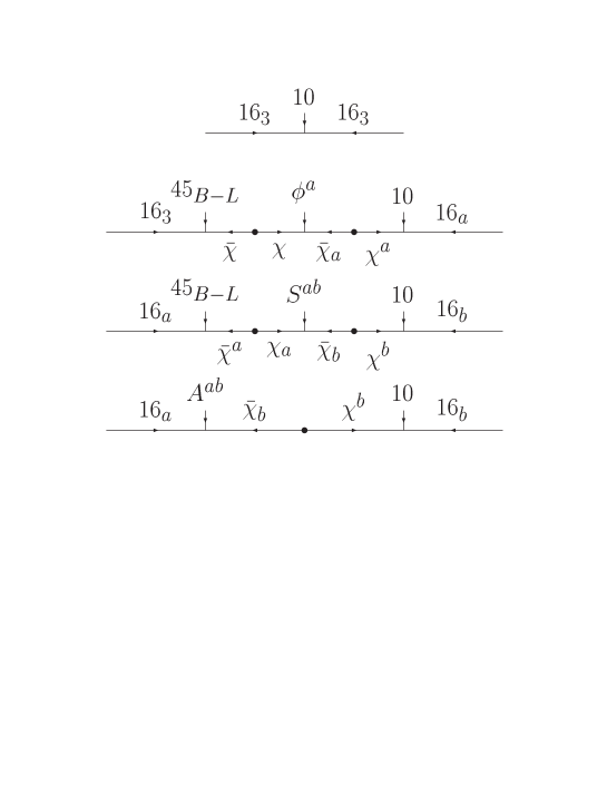
Figure 1: Diagrams generating the Yukawa matrices

In our notation, fermion doublets are on the left and singlets are on the right. Note, we have assumed that the Higgs doublets of the minimal supersymmetric standard model[MSSM] are contained in a single $10$ dimensional SO(10) multiplet. Hence all the fits have large values of $\tan\beta$. 

2.1 Results for Charged Fermion Masses and Mixing Angles

Table 1: Charged fermion masses and mixing angles
Initial parameters: $\kappa_{1}=\kappa_{2}=0$      (1/$\alpha_{G},\,M_{G},\,\epsilon_{3}$) = ($24.52,\,3.03\cdot 10^{16}$ GeV,$\,-4.06$%),
($\lambda,\,$r$,\,\sigma,\,\epsilon,\,\rho,\,\epsilon^{\prime}$) = ($0.79,\,12.4,\,0.84,\,0.011,\,0.043,\,0.0031$),
($\Phi_{\sigma},\,\Phi_{\epsilon},\,\Phi_{\rho}$) = ($0.73,\,-1.21,\,3.72$)rad,
($m_{0},\,M_{1/2},\,A_{0},\,\mu(M_{Z})$) = ($1000,\,300,\,-1431,\,110$) GeV,
($(m_{H_{d}}/m_{0})^{2},\,(m_{H_{u}}/m_{0})^{2},\,$tan$\beta$) = ($2.23,\,1.66,\,53.7$)

$$\begin{array}[]{|l|c|l|}\hline\cr{\rm Observable}&{\rm Data}(\sigma)&Theory\\ \mbox{ }&{\rm(masses}&{\rm in\ \ GeV)}\\ \hline\cr\;\;\;M_{Z}&91.187\ (0.091)&91.17\\ \;\;\;M_{W}&80.388\ (0.080)&80.39\\ \;\;\;G_{\mu}\cdot 10^{5}&1.1664\ (0.0012)&1.166\\ \;\;\;\alpha_{EM}^{-1}&137.04\ (0.14)&137.0\\ \;\;\;\alpha_{s}(M_{Z})&0.1190\ (0.003)&0.1174\\ \;\;\;\rho_{new}\cdot 10^{3}&-0.20\ (1.1)&+0.314\\ \hline\cr\;\;\;M_{t}&173.8\ (5.0)&174.9\\ \;\;\;m_{b}(M_{b})&4.260\ (0.11)&4.331\\ \;\;\;M_{b}-M_{c}&3.400\ (0.2)&3.426\\ \;\;\;m_{s}&0.180\ (0.050)&0.147\\ \;\;\;m_{d}/m_{s}&0.050\ (0.015)&0.0589\\ \;\;\;Q^{-2}&0.00203\ (0.00020)&0.00201\\ \;\;\;M_{\tau}&1.777\ (0.0018)&1.777\\ \;\;\;M_{\mu}&0.10566\ (0.00011)&.1057\\ \;\;\;M_{e}\cdot 10^{3}&0.5110\ (0.00051)&0.5110\\ \;\;\;V_{us}&0.2205\ (0.0026)&0.2205\\ \;\;\;V_{cb}&0.03920\ (0.0030)&0.0403\\ \;\;\;V_{ub}/V_{cb}&0.0800\ (0.02)&0.0691\\ \;\;\;\hat{B}_{K}&0.860\ (0.08)&0.870\\ \hline\cr{B(b\!\rightarrow\!s\gamma)\!\cdot\!10^{4}}&3.000\ (0.47)&2.992\\ \hline\cr\vrule\lx@intercol{\rm TOTAL}\;\;\;\;\chi^{2}\hfil\lx@intercol 2.26&\\ \hline\cr\end{array}$$

We have performed a global $\chi^{2}$ analysis, incorporating two (one) loop renormalization group[RG] running of dimensionless (dimensionful) parameters from $M_{G}$ to $M_{Z}$ in the MSSM, one loop radiative threshold corrections at $M_{Z}$, and 3 loop QCD (1 loop QED) RG running below $M_{Z}$. Electroweak symmetry breaking is obtained self-consistently from the effective potential at one loop, with all one loop threshold corrections included. This analysis is performed using the code of Blazek et.al. [15].  In this paper, we just present the results for one set of soft SUSY breaking parameters $m_{0},\;M_{1/2}$ with all other parameters varied to obtain the best fit solution. In the first two columns of table  1 we give the 20 observables which enter the $\chi^{2}$ function, their experimental values and the uncertainty $\sigma$ (in parentheses). In most cases $\sigma$ is determined by the 1 standard deviation experimental uncertainty, however in some cases the theoretical uncertainty ($\sim$ 0.1%) inherent in our renormalization group running and one loop threshold corrections dominates. Lastly, in contrast to paper I we include a 1999 updated value  [22] of $\rho_{new}$, the measure of SU(2) violation beyond the standard model. This change substantially improves our global charged fermion fits.

There are 8 real Yukawa parameters and 5 complex phases. We take the complex phases to be $\Phi_{\rho},\;\Phi_{\epsilon},\;\Phi_{\sigma},\;\Phi_{\kappa_{1}}$ and $\Phi_{\kappa_{2}}$. With 13 fermion mass observables (charged fermion masses and mixing angles [$\hat{B}_{K}$ replacing $\epsilon_{K}$ as a “measure of CP violation”  ]) we have enough parameters to fit the data. In table  1 we also show the fits obtained with $\kappa_{1}=\kappa_{2}=0$ as a benchmark for the cases with non-zero $\kappa_{1,2}$ which follow. From table  1 it is clear that this theory fits the low energy data quite well. 

Finally, the squark, slepton, Higgs and gaugino spectrum of our theory is consistent with all available data. The lightest chargino and neutralino are higgsino-like with the masses close to their respective experimental limits. As an example of the additional predictions of this theory consider the CP violating mixing angles which may soon be observed at B factories. For the selected fit with $\kappa_{1}=\kappa_{2}=0$ we find

$$(\sin 2\alpha,\,\sin 2\beta,\,\sin\gamma)= (0.74,\,0.54,\,0.99)$$ (22)

or equivalently the Wolfenstein parameters

$$(\rho,\,\eta)= (-0.04,\,0.31)$$ . (23)

As an aside, we have also computed the SUSY contribution to the muon anomalous magnetic moment. Our prediction for the selected SUSY point  gives values for $a_{\mu}^{SUSY}\approx 40\cdot 10^{-10}$, in good agreement with the latest preliminary data from the ongoing BNL experiment  [25].

In tables  2 - 5 we give results for non-zero $\kappa_{1},\;\kappa_{2}$. These results have been obtained with a slightly different procedure than previously. We have followed a multi step iterative procedure for finding “good” fits to both charged fermion and neutrino data. This is in lieu of combining the neutrino and charged fermion sectors into a single $\chi^{2}$ function and minimizing the total $\chi^{2}$ with respect to variations of all the parameters. Let us now describe this procedure in more detail.

In each case we select a pair of non-zero values for $\kappa_{1}$ and $\kappa_{2}$ and keep these two parameters fixed while we repeat the charged fermion analysis. If we obtain a good fit, we use these as initial values for the analysis of the neutrino sector (discussed in the next section). Then in the neutrino analysis we only vary those parameters not already included in the charged fermion analysis. If the resulting neutrino fit is not acceptable, we make a step in the ($\kappa_{1},\;\kappa_{2}$) parameter space and start again with the charged fermion analysis. We also found that we can improve the neutrino fit for fixed $\kappa_{1}$ and $\kappa_{2}$ if we return to the charged fermion analysis and carefully move one or more parameters entering the Yukawa matrices slightly away from their best fit value (watching so as not to incur large changes in the charged fermion contributions to $\chi^{2}$). Thus our tables  2 - 5 do not show the absolute “best” fits for fixed $\kappa_{1}$ and $\kappa_{2}$. Following this procedure we focus independently on different neutrino solutions as indicated in the table captions. Thus although the data in tables  2 - 5 do not seem much different, they do however represent significant changes in the neutrino sector; discussed in the next section.

Table 2: Charged fermion masses and mixing angles: 3 neutrino SMA MSW
Initial parameters: $\kappa_{1}=\kappa_{2}^{2}$, $|\kappa_{2}|=0.028$      (1/$\alpha_{G},\,M_{G},\,\epsilon_{3}$) = ($24.52,\,3.05\cdot 10^{16}$ GeV,$\,-4.07$%),
($\lambda,\,$r$,\,\sigma,\,\epsilon,\,\rho,\,\epsilon^{\prime}$) = ($0.79,\,12.3,\,-0.96,\,0.010,\,0.042,\,0.0031$),
($\Phi_{\sigma},\,\Phi_{\epsilon},\,\Phi_{\rho},\,\Phi_{\kappa_{1}},\,\Phi_{\kappa_{2}}$) = ($3.84,\,0.0032,\,5.02,\,-1.70,\,-0.85$)rad,
($m_{0},\,M_{1/2},\,A_{0},\,\mu(M_{Z})$) = ($1000,\,300,\,-1438,\,110$) GeV,
($(m_{H_{d}}/m_{0})^{2},\,(m_{H_{u}}/m_{0})^{2},\,$tan$\beta$) = ($2.22,\,1.66,\,53.7$)

$$\begin{array}[]{|l|c|l|}\hline\cr{\rm Observable}&{\rm Data}(\sigma)&Theory\\ \mbox{ }&{\rm(masses}&{\rm in\ \ GeV)}\\ \hline\cr\;\;\;M_{Z}&91.187\ (0.091)&91.18\\ \;\;\;M_{W}&80.388\ (0.080)&80.40\\ \;\;\;G_{\mu}\cdot 10^{5}&1.1664\ (0.0012)&1.166\\ \;\;\;\alpha_{EM}^{-1}&137.04\ (0.14)&137.0\\ \;\;\;\alpha_{s}(M_{Z})&0.1190\ (0.003)&0.1174\\ \;\;\;\rho_{new}\cdot 10^{3}&-0.20\ (1.1)&+0.322\\ \hline\cr\;\;\;M_{t}&173.8\ (5.0)&175.0\\ \;\;\;m_{b}(M_{b})&4.260\ (0.11)&4.326\\ \;\;\;M_{b}-M_{c}&3.400\ (0.2)&3.432\\ \;\;\;m_{s}&0.180\ (0.050)&0.146\\ \;\;\;m_{d}/m_{s}&0.050\ (0.015)&0.0585\\ \;\;\;Q^{-2}&0.00203\ (0.00020)&0.00201\\ \;\;\;M_{\tau}&1.777\ (0.0018)&1.776\\ \;\;\;M_{\mu}&0.10566\ (0.00011)&.1057\\ \;\;\;M_{e}\cdot 10^{3}&0.5110\ (0.00051)&0.5110\\ \;\;\;V_{us}&0.2205\ (0.0026)&0.2206\\ \;\;\;V_{cb}&0.03920\ (0.0030)&0.0402\\ \;\;\;V_{ub}/V_{cb}&0.0800\ (0.02)&0.0702\\ \;\;\;\hat{B}_{K}&0.860\ (0.08)&0.8691\\ \hline\cr{B(b\!\rightarrow\!s\gamma)\!\cdot\!10^{4}}&3.000\ (0.47)&2.958\\ \hline\cr\vrule\lx@intercol{\rm TOTAL}\;\;\;\;\chi^{2}\hfil\lx@intercol 2.48&\\ \hline\cr\end{array}$$

Table 3: Charged fermion masses and mixing angles: 3 neutrino LMA MSW
Initial parameters: $|\kappa_{1}|=0.055$, $|\kappa_{2}|=0.31$      (1/$\alpha_{G},\,M_{G},\,\epsilon_{3}$) = ($24.52,\,3.05\cdot 10^{16}$ GeV,$\,-4.08$%),
($\lambda,\,$r$,\,\sigma,\,\epsilon,\,\rho,\,\epsilon^{\prime}$) = ($0.79,\,14.3,\,-1.13,\,0.009,\,0.045,\,0.0028$),
($\Phi_{\sigma},\,\Phi_{\epsilon},\,\Phi_{\rho},\,\Phi_{\kappa_{1}},\,\Phi_{\kappa_{2}}$) = ($3.82,\,-0.69,\,4.83,\,4.07,\,-1.14$)rad,
($m_{0},\,M_{1/2},\,A_{0},\,\mu(M_{Z})$) = ($1000,\,300,\,-1444,\,110$) GeV,
($(m_{H_{d}}/m_{0})^{2},\,(m_{H_{u}}/m_{0})^{2},\,$tan$\beta$) = ($2.22,\,1.66,\,53.7$)

$$\begin{array}[]{|l|c|l|}\hline\cr{\rm Observable}&{\rm Data}(\sigma)&Theory\\ \mbox{ }&{\rm(masses}&{\rm in\ \ GeV)}\\ \hline\cr\;\;\;M_{Z}&91.187\ (0.091)&91.18\\ \;\;\;M_{W}&80.388\ (0.080)&80.40\\ \;\;\;G_{\mu}\cdot 10^{5}&1.1664\ (0.0012)&1.166\\ \;\;\;\alpha_{EM}^{-1}&137.04\ (0.14)&137.0\\ \;\;\;\alpha_{s}(M_{Z})&0.1190\ (0.003)&0.1174\\ \;\;\;\rho_{new}\cdot 10^{3}&-0.20\ (1.1)&+0.322\\ \hline\cr\;\;\;M_{t}&173.8\ (5.0)&174.9\\ \;\;\;m_{b}(M_{b})&4.260\ (0.11)&4.323\\ \;\;\;M_{b}-M_{c}&3.400\ (0.2)&3.433\\ \;\;\;m_{s}&0.180\ (0.050)&0.138\\ \;\;\;m_{d}/m_{s}&0.050\ (0.015)&0.0664\\ \;\;\;Q^{-2}&0.00203\ (0.00020)&0.00202\\ \;\;\;M_{\tau}&1.777\ (0.0018)&1.776\\ \;\;\;M_{\mu}&0.10566\ (0.00011)&.1057\\ \;\;\;M_{e}\cdot 10^{3}&0.5110\ (0.00051)&0.5110\\ \;\;\;V_{us}&0.2205\ (0.0026)&0.2204\\ \;\;\;V_{cb}&0.03920\ (0.0030)&0.0409\\ \;\;\;V_{ub}/V_{cb}&0.0800\ (0.02)&0.0782\\ \;\;\;\hat{B}_{K}&0.860\ (0.08)&0.8682\\ \hline\cr{B(b\!\rightarrow\!s\gamma)\!\cdot\!10^{4}}&3.000\ (0.47)&2.999\\ \hline\cr\vrule\lx@intercol{\rm TOTAL}\;\;\;\;\chi^{2}\hfil\lx@intercol 3.99&\\ \hline\cr\end{array}$$

Table 4: Charged fermion masses and mixing angles: 3 neutrino Vacuum
Initial parameters: $|\kappa_{1}|=0.004$, $|\kappa_{2}|=0.025$     (1/$\alpha_{G},\,M_{G},\,\epsilon_{3}$) = ($24.52,\,3.05\cdot 10^{16}$ GeV,$\,-4.16$%),
($\lambda,\,$r$,\,\sigma,\,\epsilon,\,\rho,\,\epsilon^{\prime}$) = ($0.80,\,15.6,\,-0.35,\,0.013,\,0.041,\,0.0035$),
($\Phi_{\sigma},\,\Phi_{\epsilon},\,\Phi_{\rho},\,\Phi_{\kappa_{1}},\,\Phi_{\kappa_{2}}$) = ($3.00,\,-0.65,\,4.41,\,3.74,\,-0.052$)rad,
($m_{0},\,M_{1/2},\,A_{0},\,\mu(M_{Z})$) = ($1000,\,300,\,-1433,\,110$) GeV,
($(m_{H_{d}}/m_{0})^{2},\,(m_{H_{u}}/m_{0})^{2},\,$tan$\beta$) = ($2.22,\,1.66,\,53.7$)

$$\begin{array}[]{|l|c|l|}\hline\cr{\rm Observable}&{\rm Data}(\sigma)&Theory\\ \mbox{ }&{\rm(masses}&{\rm in\ \ GeV)}\\ \hline\cr\;\;\;M_{Z}&91.187\ (0.091)&91.18\\ \;\;\;M_{W}&80.388\ (0.080)&80.40\\ \;\;\;G_{\mu}\cdot 10^{5}&1.1664\ (0.0012)&1.166\\ \;\;\;\alpha_{EM}^{-1}&137.04\ (0.14)&137.0\\ \;\;\;\alpha_{s}(M_{Z})&0.1190\ (0.003)&0.1171\\ \;\;\;\rho_{new}\cdot 10^{3}&-0.20\ (1.1)&+0.322\\ \hline\cr\;\;\;M_{t}&173.8\ (5.0)&175.0\\ \;\;\;m_{b}(M_{b})&4.260\ (0.11)&4.324\\ \;\;\;M_{b}-M_{c}&3.400\ (0.2)&3.405\\ \;\;\;m_{s}&0.180\ (0.050)&0.170\\ \;\;\;m_{d}/m_{s}&0.050\ (0.015)&0.0548\\ \;\;\;Q^{-2}&0.00203\ (0.00020)&0.00202\\ \;\;\;M_{\tau}&1.777\ (0.0018)&1.776\\ \;\;\;M_{\mu}&0.10566\ (0.00011)&.1057\\ \;\;\;M_{e}\cdot 10^{3}&0.5110\ (0.00051)&0.5110\\ \;\;\;V_{us}&0.2205\ (0.0026)&0.2205\\ \;\;\;V_{cb}&0.03920\ (0.0030)&0.0392\\ \;\;\;V_{ub}/V_{cb}&0.0800\ (0.02)&0.0758\\ \;\;\;\hat{B}_{K}&0.860\ (0.08)&0.8604\\ \hline\cr{B(b\!\rightarrow\!s\gamma)\!\cdot\!10^{4}}&3.000\ (0.47)&2.938\\ \hline\cr\vrule\lx@intercol{\rm TOTAL}\;\;\;\;\chi^{2}\hfil\lx@intercol 1.47&\\ \hline\cr\end{array}$$

Table 5: Charged fermion masses and mixing angles: 4 neutrino SMA MSW + LSND
Initial parameters: $|\kappa_{1}|=0.0001$, $|\kappa_{2}|=0.002$      (1/$\alpha_{G},\,M_{G},\,\epsilon_{3}$) = ($24.50,\,3.07\cdot 10^{16}$ GeV,$\,-4.14$%),
($\lambda,\,$r$,\,\sigma,\,\epsilon,\,\rho,\,\epsilon^{\prime}$) = ($0.75,\,12.4,\,-0.76,\,0.011,\,0.044,\,0.0032$),
($\Phi_{\sigma},\,\Phi_{\epsilon},\,\Phi_{\rho},\,\Phi_{\kappa_{1}},\,\Phi_{\kappa_{2}}$) = ($3.87,\,-0.95,\,3.97,\,4.81,\,1.13$)rad,
($m_{0},\,M_{1/2},\,A_{0},\,\mu(M_{Z})$) = ($1000,\,300,\,-1459,\,110$) GeV,
($(m_{H_{d}}/m_{0})^{2},\,(m_{H_{u}}/m_{0})^{2},\,$tan$\beta$) = ($2.19,\,1.65,\,53.0$)

$$\begin{array}[]{|l|c|l|}\hline\cr{\rm Observable}&{\rm Data}(\sigma)&Theory\\ \mbox{ }&{\rm(masses}&{\rm in\ \ GeV)}\\ \hline\cr\;\;\;M_{Z}&91.187\ (0.091)&91.18\\ \;\;\;M_{W}&80.388\ (0.080)&80.40\\ \;\;\;G_{\mu}\cdot 10^{5}&1.1664\ (0.0012)&1.166\\ \;\;\;\alpha_{EM}^{-1}&137.04\ (0.14)&137.0\\ \;\;\;\alpha_{s}(M_{Z})&0.1190\ (0.003)&0.1173\\ \;\;\;\rho_{new}\cdot 10^{3}&-0.20\ (1.1)&+0.318\\ \hline\cr\;\;\;M_{t}&173.8\ (5.0)&173.5\\ \;\;\;m_{b}(M_{b})&4.260\ (0.11)&4.341\\ \;\;\;M_{b}-M_{c}&3.400\ (0.2)&3.422\\ \;\;\;m_{s}&0.180\ (0.050)&0.148\\ \;\;\;m_{d}/m_{s}&0.050\ (0.015)&0.0591\\ \;\;\;Q^{-2}&0.00203\ (0.00020)&0.00201\\ \;\;\;M_{\tau}&1.777\ (0.0018)&1.776\\ \;\;\;M_{\mu}&0.10566\ (0.00011)&.1057\\ \;\;\;M_{e}\cdot 10^{3}&0.5110\ (0.00051)&0.5110\\ \;\;\;V_{us}&0.2205\ (0.0026)&0.2205\\ \;\;\;V_{cb}&0.03920\ (0.0030)&0.0402\\ \;\;\;V_{ub}/V_{cb}&0.0800\ (0.02)&0.0699\\ \;\;\;\hat{B}_{K}&0.860\ (0.08)&0.8696\\ \hline\cr{B(b\!\rightarrow\!s\gamma)\!\cdot\!10^{4}}&3.000\ (0.47)&3.007\\ \hline\cr\vrule\lx@intercol{\rm TOTAL}\;\;\;\;\chi^{2}\hfil\lx@intercol 2.94&\\ \hline\cr\end{array}$$

Table 6: Charged fermion masses and mixing angles: 5 neutrino SMA MSW + LSND
Initial parameters: $|\kappa_{1}|=|\kappa_{2}|^{2}$, $|\kappa_{2}|=0.032$      (1/$\alpha_{G},\,M_{G},\,\epsilon_{3}$) = ($24.52,\,3.06\cdot 10^{16}$ GeV,$\,-4.09$%),
($\lambda,\,$r$,\,\sigma,\,\epsilon,\,\rho,\,\epsilon^{\prime}$) = ($0.79,\,12.2,\,-0.94,\,0.011,\,0.042,\,0.0031$),
($\Phi_{\sigma},\,\Phi_{\epsilon},\,\Phi_{\rho},\,\Phi_{\kappa_{1}},\,\Phi_{\kappa_{2}}$) = ($3.84,\,0.07,\,5.03,\,-2.49,\,-1.19$)rad,
($m_{0},\,M_{1/2},\,A_{0},\,\mu(M_{Z})$) = ($1000,\,300,\,-1438,\,110$) GeV,
($(m_{H_{d}}/m_{0})^{2},\,(m_{H_{u}}/m_{0})^{2},\,$tan$\beta$) = ($2.22,\,1.66,\,53.7$)

$$\begin{array}[]{|l|c|l|}\hline\cr{\rm Observable}&{\rm Data}(\sigma)&Theory\\ \mbox{ }&{\rm(masses}&{\rm in\ \ GeV)}\\ \hline\cr\;\;\;M_{Z}&91.187\ (0.091)&91.17\\ \;\;\;M_{W}&80.388\ (0.080)&80.40\\ \;\;\;G_{\mu}\cdot 10^{5}&1.1664\ (0.0012)&1.166\\ \;\;\;\alpha_{EM}^{-1}&137.04\ (0.14)&137.0\\ \;\;\;\alpha_{s}(M_{Z})&0.1190\ (0.003)&0.1174\\ \;\;\;\rho_{new}\cdot 10^{3}&-0.20\ (1.1)&+0.322\\ \hline\cr\;\;\;M_{t}&173.8\ (5.0)&175.0\\ \;\;\;m_{b}(M_{b})&4.260\ (0.11)&4.328\\ \;\;\;M_{b}-M_{c}&3.400\ (0.2)&3.426\\ \;\;\;m_{s}&0.180\ (0.050)&0.148\\ \;\;\;m_{d}/m_{s}&0.050\ (0.015)&0.0588\\ \;\;\;Q^{-2}&0.00203\ (0.00020)&0.00201\\ \;\;\;M_{\tau}&1.777\ (0.0018)&1.777\\ \;\;\;M_{\mu}&0.10566\ (0.00011)&.1057\\ \;\;\;M_{e}\cdot 10^{3}&0.5110\ (0.00051)&0.5110\\ \;\;\;V_{us}&0.2205\ (0.0026)&0.2205\\ \;\;\;V_{cb}&0.03920\ (0.0030)&0.0401\\ \;\;\;V_{ub}/V_{cb}&0.0800\ (0.02)&0.0701\\ \;\;\;\hat{B}_{K}&0.860\ (0.08)&0.8686\\ \hline\cr{B(b\!\rightarrow\!s\gamma)\!\cdot\!10^{4}}&3.000\ (0.47)&2.983\\ \hline\cr\vrule\lx@intercol{\rm TOTAL}\;\;\;\;\chi^{2}\hfil\lx@intercol 2.12&\\ \hline\cr\end{array}$$

Before we conclude this section, let us consider one test (in the charged fermion sector) which may be able to distinguish among these different neutrino cases. The unitarity angles $(\sin 2\alpha,\,\sin 2\beta,\,\sin\gamma)$ or equivalently the Wolfenstein parameters $(\rho,\;\eta)$ in some cases have significant corrections depending on the neutrino solution (see table  7). In particular, for larger values of $\kappa_{1},\;\kappa_{2}$ we obtain significantly larger negative values of $\rho$; in particular consider $\rho=-0.24$ for the 3 $\nu$ LMA MSW solution. This may be severely constrained by $B-\bar{B}$ mixing data. However in order to determine whether this is consistent with present data we must first extend our numerical analysis to include this process. We will look at this in a future paper [24].

Table 7: Unitarity triangle angles and Wolfenstein parameters for the different neutrino fits with non zero $\kappa_{1},\;\kappa_{2}$.

$$\begin{array}[]{|l|l|l|l|}\hline\cr{\rm Neutrino\;\;fit}&{\rm Values\;\;of}\;\kappa_{1},\;\kappa_{2}&(\sin 2\alpha,\;\sin 2\beta,\;\sin\gamma)&(\rho,\;\eta)\\ \hline\cr 3\nu\;\;\;{\rm SMA\,MSW}&\kappa_{1}=\kappa_{2}^{2},\;|\kappa_{2}|=0.028&(0.92,\;0.50,\;0.95)&(-0.10,\;0.30)\\ \hline\cr 3\nu\;\;\;{\rm LMA\,MSW}&|\kappa_{1}|=0.055,\;|\kappa_{2}|=0.31&(0.94,\;0.39,\;0.73)&(-0.24,\;0.26)\\ \hline\cr 3\nu\;\;\;{\rm Vacuum}&|\kappa_{1}|=0.004,\;|\kappa_{2}|=0.025&(0.86,\;0.56,\;0.97)&(-0.08,\;0.33)\\ \hline\cr 4\nu{\rm SMA\,MSW+LSND}&|\kappa_{1}|=0.0001,\;|\kappa_{2}|=0.002&(0.75,\;0.54,\;0.99)&(-0.04,\;0.31)\\ \hline\cr 5\nu{\rm SMA\,MSW+LSND}&|\kappa_{1}|=|\kappa_{2}|^{2},\;|\kappa_{2}|=0.032&(0.88,\;0.51,\;0.96)&(-0.09,\;0.31)\\ \hline\cr\end{array}$$

3 Neutrino Masses and Mixing Angles

The parameters in the Dirac Yukawa matrix for neutrinos (eqn.  11) mixing $\nu-\bar{\nu}$ are now fixed. Of course, neutrino masses are much too large and we need to invoke the GRSY [26] see-saw mechanism.

Since the 16 of SO(10) contains the “right-handed” neutrinos $\bar{\nu}$, one possibility is to obtain $\bar{\nu}-\bar{\nu}$ Majorana masses via higher dimension operators of the form 

$${1\over M}\ \overline{16}\ 16_{3}\ \overline{16}\ 16_{3},{1\over M^{2}}\ \overline{16}\ 16_{3}\ \overline{16}\ 16_{a}\ \phi^{a},{1\over M^{2}}\ \overline{16}\ 16_{a}\ \overline{16}\ 16_{b}\ S^{a\,b}.$$ (24)

The second possibility, which we follow, is to introduce SO(10) singlet fields $N$ and obtain effective mass terms $\bar{\nu}-N$ and $N-N$ using only dimension four operators in the superspace potential. To do this, we add three new SO(10) singlets {$N_{a},\;a=1,2;\;\;N_{3}$} with U(1) charges { $-1/2$,  +1/2 }. These then contribute to the superspace potential

$$W\supset\overline{16}\;(N_{a}\;\chi^{a}\;\;+\;\;N_{3}\;16_{3})+{1\over 2}\ N_{a}\;N_{b}\;S^{a\;b}\;\;+\;\;N_{a}\;N_{3}\;\phi^{a}$$ (25)

where the field $\overline{16}$ with U(1) charge $-1/2$ is assumed to get a vev in the “right-handed” neutrino direction. Note, this vev is also needed to break the rank of SO(10).

Finally we allow for the possibility of adding a U(2) doublet of SO(10) singlets $\bar{N}^{a}$ or a U(2) singlet $\bar{N}^{3}$. They enter the superspace potential as follows –

$$W\supset \mu^{\prime}\;N_{a}\;\bar{N}^{a}\;\;+\;\;\mu_{3}\;N_{3}\bar{N}^{3}$$ (26)

The dimensionful parameters $\mu^{\prime},\;\mu_{3}$ are assumed to be of order the weak scale. The notation is suggestive of the similarity between these terms and the $\mu$ term in the Higgs sector. In both cases, we are adding supersymmetric mass terms and in both cases, we need some mechanism to keep these dimensionful parameters small compared to the Planck scale.

We define the 3 $\times$ 3 matrix

$$\tilde{\mu}= \left(\begin{array}[]{ccc}\mu^{\prime}&0&0\\ 0&\mu^{\prime}&0\\ 0&0&\mu_{3}\end{array}\right)$$ (30)

The matrix $\tilde{\mu}$ determines the number of coupled sterile neutrinos, i.e. there are 4 cases labeled by the number of neutrinos ($N_{\nu}=3,4,5,6$):

• ($N_{\nu}=3$)   3 active     ($\mu^{\prime}=\mu_{3}=0$);

• ($N_{\nu}=4$)   3 active + 1 sterile

  ($\mu^{\prime}=0;\;\mu_{3}\neq 0$);

• ($N_{\nu}=5$)   3 active + 2 sterile

  ($\mu^{\prime}\neq 0;\;\mu_{3}=0$);

• ($N_{\nu}=6$)   3 active + 3 sterile

  ($\mu^{\prime}\neq 0;\;\mu_{3}\neq 0$);

In this paper we consider the cases $N_{\nu}=3$, 4 and 5.

The generalized neutrino mass matrix is then given by 

$$(\begin{array}[]{cccc}\;\nu&\;\;\bar{N}&\;\;\bar{\nu}&\;\;N\end{array})$$ (32)

$$\left(\begin{array}[]{cccc}0&0&m&0\\ 0&0&0&\tilde{\mu}^{T}\\ m^{T}&0&0&V\\ 0&\tilde{\mu}&V^{T}&M_{N}\end{array}\right)$$ (37)

where

$$m= Y_{\nu}\;\langle H_{u}^{0}\rangle =\;Y_{\nu}\;{v\over\sqrt{2}}\;\sin\beta$$ (38)

and

$$V= \left(\begin{array}[]{ccc}3\,\kappa_{1}\,\epsilon\,V_{16}&(\epsilon^{\prime}+3\,\kappa_{2}\,\epsilon)\,V_{16}&0\\ -(\epsilon^{\prime}-3\,\kappa_{2}\,\epsilon)\,V_{16}&3\epsilon V_{16}&0\\ 0&r\,\epsilon\,(1-\sigma)\,T_{\bar{\nu}}V_{16}&V^{\prime}_{16}\end{array}\right)$$ (42)

$$M_{N}= \left(\begin{array}[]{ccc}\kappa_{1}\,S&\kappa_{2}\,S&0\\ \kappa_{2}\,S&S&\phi\\ 0&\phi&0\end{array}\right)$$ (46)

$V_{16},\;V^{\prime}_{16}$ are proportional to the vev of $\overline{16}$ (with different implicit Yukawa couplings) and $S,\;\phi$ are up to couplings the vevs of $S^{22},\;\phi^{2}$, respectively.

Since both $V$ and $M_{N}$ are of order the GUT scale, the states $\bar{\nu},\;N$ may be integrated out of the effective low energy theory. In this case, the effective neutrino mass matrix is given (at $M_{G}$) by  (the matrix is written in the ($\nu,\ \bar{N}$) flavor basis where charged lepton masses are diagonal)

$$m_{\nu}=\tilde{U}_{e}^{T}\;\left(\begin{array}[]{cc}m\;(V^{T})^{-1}\;M_{N}\;V^{-1}\;m^{T}&-m\;(V^{T})^{-1}\;\tilde{\mu}\\ -{\tilde{\mu}}^{T}\;V^{-1}\;m^{T}&0\end{array}\right)\;\tilde{U}_{e}$$ (47)

with

$$\tilde{U}_{e}= \left(\begin{array}[]{cc}U_{e}&0\\ 0&1\end{array}\right)$$ (50)

$$e_{0}=U_{e}\;e\;\;; \nu_{0}=U_{e}\;\nu$$

$U_{e}$ is the $3\times 3$ unitary matrix for left-handed leptons needed to diagonalize $Y_{e}$ (eqn. 11) and $e_{0},\;\nu_{0}\;(e,\;\nu)$ represent the three families of left-handed leptons in the charged-weak ( -mass) eigenstate basis.

The neutrino mass matrix is diagonalized by a unitary matrix $U=U_{\alpha\,i}$;

$$m^{diag}_{\nu}= U^{T}\;m_{\nu}\;U$$ (51)

where $\alpha=\{\nu_{e},\;\nu_{\mu},\;\nu_{\tau},\;\nu_{s_{1}},\;\nu_{s_{2}},\;\nu_{s_{3}}\}$ is the flavor index and $i=\{1,\cdots,6\}$ is the neutrino mass eigenstate index. $U_{\alpha\,i}$ is observable in neutrino oscillation experiments. In particular, the probability for the flavor state $\nu_{\alpha}$ with energy $E$ to oscillate into $\nu_{\beta}$ after travelling a distance $L$ is given by

$$P(\nu_{\alpha}\rightarrow\nu_{\beta})=\delta_{\alpha\beta}-4\sum_{k\;<\,j}U_{\alpha\,k}\ U^{*}_{\beta\,k}\ U^{*}_{\alpha\,j}\ U_{\beta\,j}\ \sin^{2}\Delta_{j\,k}$$ (52)

where $\Delta_{j\,k}={\delta m^{2}_{jk}\ L\over 4E}$ and $\delta m^{2}_{jk}=m^{2}_{j}-m^{2}_{k}$.

For N${}_{\nu}\leq 4$ we have

$$m_{\nu}=m^{\prime}\;\tilde{U}_{e}^{T}\;\left(\begin{array}[]{cccc}\kappa_{1}\,\omega\,\zeta&\kappa_{2}\,\omega\,\zeta&\frac{\kappa_{1}\,\epsilon\,\epsilon^{\prime}\,r\,\sigma}{\bar{\epsilon}^{2}}\,\zeta&0\\ \kappa_{2}\,\omega\,\zeta&b&C_{23}&-u\,c\\ \frac{\kappa_{1}\,\epsilon\,\epsilon^{\prime}\,r\,\sigma}{\bar{\epsilon}^{2}}\,\zeta&C_{23}&C_{33}&-f\,c\\ 0&-u\,c&-f\,c&0\end{array}\right)\;\tilde{U}_{e}$$ (53)

where

$$\zeta= ({S\ V^{\prime}_{16}\over\phi\ V_{16}})$$ (54)

$$b= \omega\ \zeta+2\ \sigma\ r\ \epsilon$$

$$\bar{\epsilon}^{2}= (\epsilon^{\prime})^{2}+9\,(\kappa_{1}-\kappa_{2}^{2})\,\epsilon^{2}$$

$$C_{23}= \left(1+\frac{3}{2}\,\frac{\kappa_{1}\,\epsilon^{3}\,r^{2}\,\sigma\,(3-4\sigma)}{\bar{\epsilon}^{2}}\right)-\frac{3\,(\kappa_{1}-\kappa_{2}^{2})\,\epsilon^{2}-\kappa_{2}\,\epsilon\,\epsilon^{\prime}}{\bar{\epsilon}^{2}}\,r\,\sigma\,\zeta$$

$$C_{33}= -\frac{6\,\kappa_{1}\,\epsilon^{2}\,r\,\sigma}{\bar{\epsilon}^{2}\,\omega}\,\left(1+\frac{3\,\kappa_{1}\,\epsilon^{3}\,r^{2}\,\sigma\,(1-\sigma)}{\bar{\epsilon}^{2}}\right)+\frac{\kappa_{1}\,\epsilon^{2}\,r^{2}\,\sigma^{2}}{\bar{\epsilon}^{2}\,\omega}\,\zeta$$

$$u= r\,\sigma\,\epsilon$$

$$c= \frac{\mu_{3}\,V_{16}}{\omega\,m_{t}\,\phi}$$

$$f= 1+\frac{3\epsilon^{3}\kappa_{1}r^{2}\sigma(1-\sigma)}{\bar{\epsilon}^{2}}$$

and

$$m^{\prime} = \frac{\lambda^{2}v^{2}\sin^{2}\beta~{}\omega\phi}{2V_{16}V^{\prime}_{16}}\approx{m_{t}^{2}\ \omega\ \phi\over V_{16}\ V^{\prime}_{16}}$$ (55)

where in the approximation for $m^{\prime}$ we use

$$m_{t}(\equiv m_{top})\approx\lambda\ {v\over\sqrt{2}}\ \sin\beta,$$ (56)

valid at the weak scale.

In addition, for $N_{\nu}=5$ the off-diagonal piece of the mass matrix in eq.(47) reads

$$-{\tilde{\mu}}^{T}\,V^{-1}\>m^{T}=-m^{\prime}\;d\;\left(\begin{array}[]{ccc}1&0&(u-r\epsilon/2)\,g\\ 0&1&(u-r\epsilon/2)\,h\end{array}\right),$$ (57)

with

$$d = \frac{\mu^{\prime}\;V_{16}^{\prime}}{m_{t}\;\phi}$$ (58)

$$g = (3\epsilon\kappa_{2}+\epsilon^{\prime})/\bar{\epsilon}^{2}$$ (59)

$$h = -3\epsilon\kappa_{1}/\bar{\epsilon}^{2}.$$ (60)

3.1 Three Neutrinos

Before we discuss the case with non-zero $\kappa_{(1,2)}$, let’s recall the problem when $\kappa_{(1,2)}=0$. For three active neutrinos with minimal family breaking vevs, $\langle\phi^{2}\rangle,\;\langle S^{22}\rangle,\;\langle A^{12}\rangle\neq 0$ and $\kappa_{1}=\kappa_{2}=0$, we find (at $M_{G}$) in the ($\nu_{e},\;\nu_{\mu},\;\nu_{\tau}$) basis

$$m_{\nu}=m^{\prime}\;U_{e}^{T}\;\left(\begin{array}[]{ccc}0&0&0\\ 0&b&1\\ 0&1&0\end{array}\right)\;U_{e}$$ (64)

$m_{\nu}$ is given in terms of two independent parameters { $m^{\prime},\;b$ } (see equations  54,  55). Note, this theory in principle solves two problems associated with neutrino masses. It naturally has small mixing between $\nu_{e}-\nu_{\mu}$ since the mixing angle comes purely from diagonalizing the charged lepton mass matrix which, like quarks, has small mixing angles. While, for $b\leq 1$, $\nu_{\mu}-\nu_{\tau}$ mixing is large without fine tuning. Also note, in this theory one neutrino (predominantly $\nu_{e}$) is massless.

We have checked that in this theory it is possible to simultaneously fit both atmospheric and LSND data. We however cannot simultaneously fit both solar and atmospheric neutrino data. As discussed in paper I [14] this problem can be solved at the expense of adding a new family symmetry breaking vev 

$$\langle\phi^{1}\rangle=\kappa\langle\phi^{2}\rangle.$$ (65)

In this paper we consider the most general family symmetry breaking vevs, given in equation  1, introducing two new complex parameters $\kappa_{1},\;\kappa_{2}$. This allows us to obtain a small mass difference between the first and second mass eigenvalues which was unattainable before in the large mixing limit for $\nu_{\mu}-\nu_{\tau}$. Hence good fits to both solar and atmospheric neutrino data can now be found. In addition, in the previous section we showed that small values of $\kappa_{1,2}$ are consistent with good fits for charged fermion masses and mixing angles. In the next section we discuss these new solutions.

4 Neutrino oscillations [ 3 active only ]

In this section we consider the solutions to atmospheric and solar neutrino oscillations with three neutrinos. The mass matrix is given in equation  53 with the parameter $c=0$. There are three possible solutions to the solar neutrino data defined as small mixing angle [SMA] MSW, large mixing angle [LMA] MSW or “Just so” vacuum oscillations [6]. In all three cases atmospheric neutrino data are predominantly described by $\nu_{\mu}\rightarrow\nu_{\tau}$ oscillations.

Instead of fitting the data directly, we compare our models with existing 2 neutrino oscillation fits to the data [6]. We use the latest two neutrino fits to the most recent Super-Kamiokande data for atmospheric neutrino oscillations and the best fits to solar neutrino data including the possibility of “just so” vacuum oscillations or both large and small angle MSW oscillations [2, 1, 6].

For atmospheric neutrino oscillations we have evaluated the probabilities ($P(\nu_{\mu}\rightarrow\nu_{\mu})$, $P(\nu_{\mu}\rightarrow\nu_{x})\ {\rm with}\ x=\{e,\ \tau,\ s\}$) as a function of ${\rm x}\equiv\rm{Log}[(L/km)/(E/GeV)]$. In order to smooth out the oscillations we have averaged the result over a bin size, $\Delta$x = 0.5. In figures 2a and 4a we see that our results are in good agreement with the values of $\delta m^{2}_{atm}$ and $\sin^{2}2\theta_{atm}$ as given.

For solar neutrinos we plot, in figures 3(a,b) and 5(a,b), the probabilities ($P(\nu_{e}\rightarrow\nu_{e})$, $P(\nu_{e}\rightarrow\nu_{x})\ {\rm with}\ x=\{\mu,\ \tau,\ s\}$) for neutrinos produced at the center of the sun to propagate to the surface (and then without change to earth), as a function of the neutrino energy E_ν (MeV).  We then compare our model to a 2 neutrino oscillation model with the given parameters.

4.1 3 $\nu$ SMA MSW solution

In tables  8 and  9 we give the parameters for the fit corresponding to figures 2(a,b) and 3(a,b). This model is indistinguishable from the results of the given parameters for 2 neutrino oscillations $\nu_{\mu}-\nu_{\tau}$ for atmospheric data and $\nu_{e}-\nu_{active}$ for solar data.

In order to obtain a SMA MSW solution we need to choose $\kappa_{1}=\kappa_{2}^{2}$ to high accuracy. Note this value of $\kappa_{(1,2)}$ corresponds to the only solution obtained previously (in I) with non zero $\kappa$ defined by $\langle\phi^{1}\rangle=\kappa\,\langle\phi^{2}\rangle$. In fact, an SU(2) rotation of this case to zero $\langle\phi^{1}\rangle$ gives non zero $\langle S^{11}\rangle,\;\langle S^{12}\rangle$ satisfying the relation $\kappa_{1}=\kappa_{2}^{2}$.

The parameter $m^{\prime}$ is determined by the high see-saw scale. Given $m^{\prime}$(eqn.  55 and table  8) we find $V_{16}V^{\prime}_{16}/\phi=1.33\cdot 10^{16}$ GeV which is consistent with the GUT scale. The large value of $b$ (eqn.  54) results from $S\sim 10\;\phi$ which is needed in order to have one large and two small eigenvalues.

Table 8: Fit to atmospheric and solar neutrino oscillations [3 $\nu$ SMA MSW]
Initial parameters: ( $\kappa_{1}=\kappa_{2}^{2}$, $|\kappa_{2}|=0.028$ )     $m^{\prime}$ = 3.35 $\cdot$10^-3 eV ,   $b$ = 15.0,   $\Phi_{b}$ = 3.30rad

$$\begin{array}[]{|c|c|}\hline\cr{\rm Observable}&{\rm Computed\;\;value}\\ \hline\cr\delta m^{2}_{atm}&3.5\cdot 10^{-3}\ \rm eV^{2}\\ \sin^{2}2\theta_{atm}&0.99\\ \delta m^{2}_{sol}&6.3\cdot 10^{-6}\ \rm eV^{2}\\ \sin^{2}2\theta_{sol}&5.2\cdot 10^{-3}\\ \hline\cr\end{array}$$

Table 9: Neutrino Masses and Mixings   [3 $\nu$ SMA MSW] Mass eigenvalues [eV]:    0.000001,  0.0025,  0.059          
Magnitude of neutrino mixing matrix U${}_{\alpha\ i}$
$i=1,\cdots,3$ – labels mass eigenstates. $\alpha=\{e,\ \mu,\ \tau\}$ labels flavor eigenstates.

$$\left[\begin{array}[]{ccc}0.997&0.0360&0.0599\\ 0.0677&0.672&0.738\\ 0.0172&0.740&0.673\\ \end{array}\right]$$

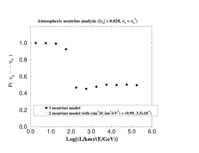
Figure 2 a: Probability $P(\nu_{\mu}\longrightarrow\nu_{\mu})$ for atmospheric neutrinos [3 $\nu$ SMA MSW]. For this analysis, we neglect the matter effects.

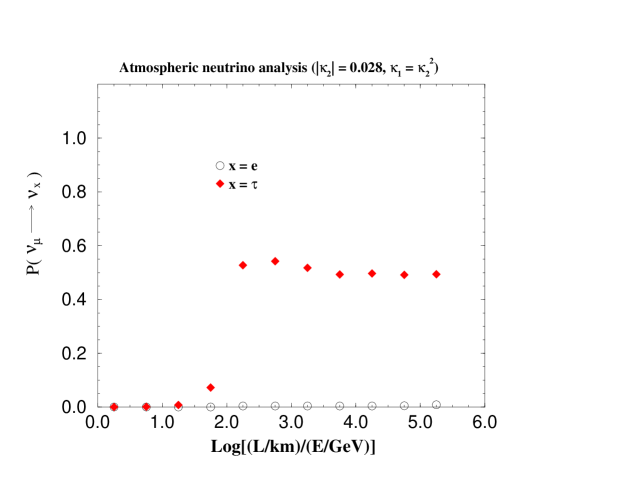
Figure 2 b: Probabilities $P(\nu_{\mu}\longrightarrow\nu_{x})$ ($x=e$, $\tau$ and $s$) for atmospheric neutrinos [3 $\nu$ SMA MSW].

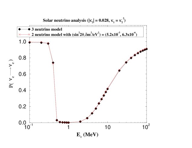
Figure 3 a: Probability $P(\nu_{e}\longrightarrow\nu_{e})$ for solar neutrinos [3 $\nu$ SMA MSW].

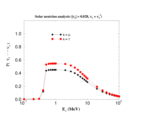
Figure 3 b: Probabilities $P(\nu_{e}\longrightarrow\nu_{x})$ ($x=\mu$, $\tau$ and $s$) for solar neutrinos [3 $\nu$ SMA MSW].

4.2 3 $\nu$ LMA MSW solution

In figures 4(a,b) and 5(a,b) we present the comparison to a two neutrino oscillation model for atmospheric and solar neutrino data (see also tables  10 and  11). For atmospheric data the fit is good for values of
$Log((L/km)/(E/GeV))\leq 4$ (see figures 4(a,b)) where the oscillations are predominantly given by $\nu_{\mu}-\nu_{\tau}$. For larger $x\geq 4$ the probability $P(\nu_{\mu}\rightarrow\nu_{\mu})$ is significantly smaller ($\sim$ 30 %) in our model than in a two neutrino model. This is due to the onset of significant $\nu_{\mu}\rightarrow\nu_{e}$ oscillations. These larger values of $x$ may be accessible in atmospheric oscillations. The maximum distance $L$ for neutrinos of order 13,000 km, for upward going neutrinos, and the minimum detectable energy of order 0.1 GeV, corresponds to a value of $x_{MAX}\sim 5$. On the other hand, it would require a much more detailed analysis to determine whether our model is consistent with the data for fully contained events in the sub GeV ( $<$ 1.33 GeV ) regime. We also note that this effect has been considered, in a recent analysis by Peres and Smirnov [29], as a possible tool to distinguish the LMA MSW solution from the other solutions to the solar neutrino problem.

Table 10: Fit to atmospheric and solar neutrino oscillations [3 $\nu$ LMA MSW]
Initial parameters: ( $|\kappa_{1}|=0.055$, $|\kappa_{2}|=0.31$ )     $m^{\prime}$ = 4.93 $\cdot$10^-2 eV ,   $b$ = 0.84,   $\Phi_{b}$ = -0.41 rad

$$\begin{array}[]{|c|c|}\hline\cr{\rm Observable}&{\rm Computed\;\;value}\\ \hline\cr\delta m^{2}_{atm}&3.7\cdot 10^{-3}\ \rm eV^{2}\\ \sin^{2}2\theta_{atm}&0.99\\ \delta m^{2}_{sol}&2.3\cdot 10^{-5}\ \rm eV^{2}\\ \sin^{2}2\theta_{sol}&0.77\\ \hline\cr\end{array}$$

Table 11: Neutrino Masses and Mixings   [3 $\nu$ LMA MSW] Mass eigenvalues [eV]:    0.002,  0.005,  0.061          
Magnitude of neutrino mixing matrix U${}_{\alpha\ i}$
$i=1,\cdots,3$ – labels mass eigenstates. $\alpha=\{e,\ \mu,\ \tau\}$ labels flavor eigenstates.

$$\left[\begin{array}[]{ccc}0.857&0.513&0.049\\ 0.368&0.563&0.740\\ 0.362&0.648&0.671\\ \end{array}\right]$$

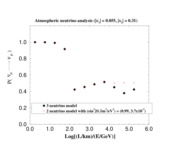
Figure 4 a: Probability $P(\nu_{\mu}\longrightarrow\nu_{\mu})$ for atmospheric neutrinos [3 $\nu$ LMA MSW]. For this analysis, we neglect the matter effects.

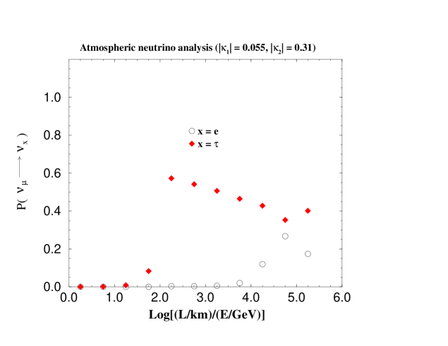
Figure 4 b: Probabilities $P(\nu_{\mu}\longrightarrow\nu_{x})$ ($x=e$, $\tau$ and $s$) for atmospheric neutrinos [3 $\nu$ LMA MSW].

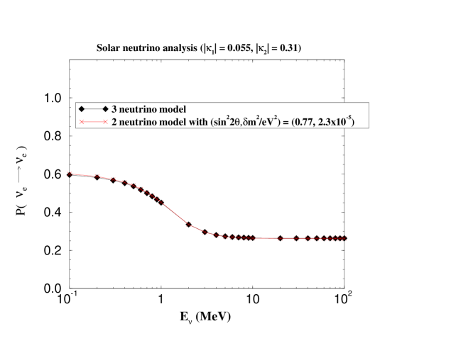
Figure 5 a: Probability $P(\nu_{e}\longrightarrow\nu_{e})$ for solar neutrinos [3 $\nu$ LMA MSW].

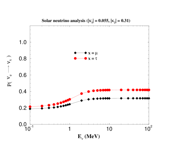
Figure 5 b: Probabilities $P(\nu_{e}\longrightarrow\nu_{x})$ ($x=\mu$, $\tau$ and $s$) for solar neutrinos [3 $\nu$ LMA MSW].

A large mixing angle oscillation solution is obtained by tuning the lightest two neutrinos to be approximately degenerate with a near bi-maximal mixing matrix (see tables  10 and  11), where the bi-maximal mixing matrix is given by [30]

$$|U_{\alpha\ i}|= \left[\begin{array}[]{ccc}0.71&0.71&0.0\\ 0.5&0.5&0.71\\ 0.5&0.5&0.71\\ \end{array}\right]$$ (69)

Note, a major difference in our case is the non-zero value for $U_{\nu_{e}3}\sim.049$. However the constraint $U_{\nu_{e}3}=0$ chosen to satisfy CHOOZ [4] is much too strong. It is easy to see that our model is consistent with the null results of CHOOZ, i.e.

$$P(\nu_{e}\rightarrow\nu_{e})= 1-4|U_{\nu_{e}3}|^{2}(1-|U_{\nu_{e}3}|^{2})sin^{2}(\frac{1.27\delta m_{atm}^{2}(eV^{2})L(km)}{E_{\nu}(GeV)}) >0.98$$

for values of $|U_{\nu_{e}3}|\leq 0.16$ [31]. Finally the parameter $b\sim 1$ requires no fine tuning and given $m^{\prime}$ we find the high see-saw scale $V_{16}V^{\prime}_{16}/\phi=8.78\cdot 10^{14}$ GeV.

4.3 3 $\nu$ “Just So” Vacuum solution

A vacuum solution is obtained by tuning the lightest two neutrinos to be even more degenerate than in the previous LMA MSW case. Our results are given in tables  12 and  13. We have not given any figures since the results are standard vacuum oscillations. Once again we obtain a near bi-maximal mixing matrix [30] with however $U_{\nu_{e}3}\sim.049$. Nevertheless this model is consistent with CHOOZ data  [4] (see the discussion of this in the LMA MSW case). Finally given the overall scale $m^{\prime}$ we determine the high energy scale to be $V_{16}V^{\prime}_{16}/\phi=2.27\cdot 10^{15}$ GeV and $b\sim 1$.

Table 12: Fit to atmospheric and solar neutrino oscillations [3 $\nu$ Vacuum]
Initial parameters: ( $|\kappa_{1}|=0.004$, $|\kappa_{2}|=0.025$ )     $m^{\prime}$ = 2.92 $\cdot$10^-2 eV ,   $b$ = 1.73,   $\Phi_{b}$ = -0.33 rad

$$\begin{array}[]{|c|c|}\hline\cr{\rm Observable}&{\rm Computed\;\;value}\\ \hline\cr\delta m^{2}_{atm}&3.5\cdot 10^{-3}\ \rm eV^{2}\\ \sin^{2}2\theta_{atm}&0.99\\ \delta m^{2}_{sol}&7.9\cdot 10^{-11}\ \rm eV^{2}\\ \sin^{2}2\theta_{sol}&0.97\\ \hline\cr\end{array}$$

Table 13: Neutrino Masses and Mixings   [3 $\nu$ Vacuum] Mass eigenvalues [eV]:    0.00106037,    0.00106041 ,  0.059          
Magnitude of neutrino mixing matrix U${}_{\alpha\ i}$
$i=1,\cdots,3$ – labels mass eigenstates. $\alpha=\{e,\ \mu,\ \tau\}$ labels flavor eigenstates.

$$\left[\begin{array}[]{ccc}0.759&0.649&0.049\\ 0.429&0.513&0.744\\ 0.489&0.563&0.667\\ \end{array}\right]$$

In the next section we discuss a four neutrino solution to atmospheric, solar and LSND neutrino data in the theory with $\kappa_{(1,2)}\neq 0$.

5 Neutrino oscillations [3 active + 1 sterile]

In the four neutrino case the mass matrix (at $M_{G}$) is given by equation  53 with $c\neq 0$.

As in the previous case of three neutrinos, we compare our model with two-neutrino oscillation models which have already been fit to the data  [1, 2, 6]. The results for our best fit are found in tables  14 and  15 and figures 6(a,b), 7(a,b) and 8.

In fig. 6a we evaluate $P(\nu_{\mu}\rightarrow\nu_{\mu})$ where we also include a multiplicative fudge factor $\alpha$. This is justified by the theoretical uncertainty in the normalization of the incident $\nu_{\mu}$ flux. Recall the observed number of muon neutrinos is given by

$$N(\nu_{\mu})= N_{0}(\nu_{\mu})\;P(\nu_{\mu}\rightarrow\nu_{\mu})$$ (71)

where $N_{0}(\nu_{\mu})$ is the theoretically expected incident neutrino flux which has an uncertainty of order 20%. We let $N_{0}(\nu_{\mu})=N_{fit}\cdot\alpha$ where $N_{fit}$ is the value used for the neutrino flux when fitting the data.

We see that our result is in good agreement with the values of $\delta m^{2}_{atm}=3.5\cdot 10^{-3}$eV² and $\sin^{2}2\theta_{atm}=1.0$ with $\alpha=1.04$.

In fig. 6b we see that the atmospheric neutrino deficit is predominantly due to the maximal mixing between $\nu_{\mu}-\nu_{\tau}$, as in the case with $\kappa_{1}=\kappa_{2}=0$. However, in the case with $\kappa_{1}=\kappa_{2}=0$ there is also a significant ($\sim$ 10% effect) oscillation of $\nu_{\mu}-\nu_{s}$. In this case, that effect has vanished. This also means that sterile neutrinos will not come into thermal equilibrium in the early universe, due to the small mixing angle. Hence, at the nucleosynthesis epoch this model has only three neutrino species in thermal equilibrium.

Table 14: Fit to atmospheric, solar and LSND neutrino oscillations [4 neutrinos   SMA MSW + LSND]
 Initial parameters: $|\kappa_{1}|=0.0001,\;|\kappa_{2}|=0.002$                            $m^{\prime}=0.979$ eV ,  $b$ = -0.054,  $c$ = 0.101, $\Phi_{b}$ = 5.59rad

$$\begin{array}[]{|c|c|}\hline\cr{\rm Observable}&{\rm Computed\;\;value}\\ \hline\cr\delta m^{2}_{atm}&3.5\cdot 10^{-3}\ \rm eV^{2}\\ \sin^{2}2\theta_{atm}&1.0\\ \delta m^{2}_{sol}&5.0\cdot 10^{-6}\ \rm eV^{2}\\ \sin^{2}2\theta_{sol}&3.0\cdot 10^{-3}\\ \delta m^{2}_{LSND}&0.53\\ \sin^{2}2\theta_{LSND}&0.018\\ \hline\cr\end{array}$$

Table 15: Neutrino Masses and Mixings [4 neutrinos   SMA MSW + LSND]
Mass eigenvalues [eV]:    0.00002,  0.0022,  0.7248,  0.7272          
Magnitude of neutrino mixing matrix U_αi                
$i=1,\cdots,4$ – labels mass eigenstates.              
$\alpha=\{e,\ \mu,\ \tau,\ s\}$ labels flavor eigenstates.

$$\left[\begin{array}[]{cccc}0.997&0.0254&0.0480&0.0482\\ 0.0703&0.1079&0.7022&0.7003\\ 0.273\cdot 10^{-3}&0.0292&0.7053&0.7083\\ 0.0181&0.9934&0.0852&0.0745\\ \end{array}\right]$$

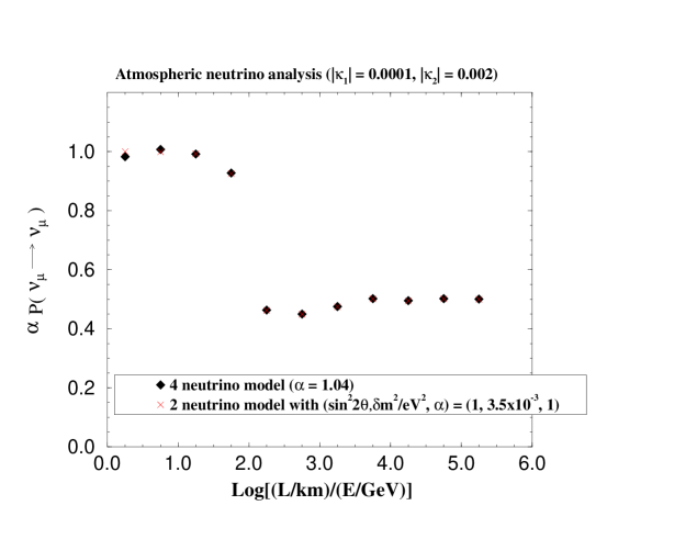
Figure 6 a: Probability $P(\nu_{\mu}\longrightarrow\nu_{\mu})$ for atmospheric neutrinos multiplied by $\alpha$, a fudge factor introduced to account for the uncertainty in the normalization of the incident $\nu_{\mu}$ flux. For this analysis, we neglect matter effects.

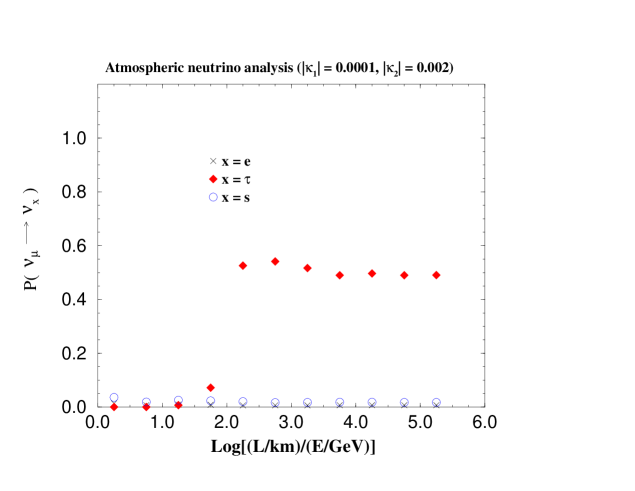
Figure 6 b: Probabilities $P(\nu_{\mu}\longrightarrow\nu_{x})$ ($x=e$, $\tau$ and $s$) for atmospheric neutrinos

For solar neutrinos we see in fig. 7a that our model reproduces the neutrino results for $\delta m^{2}_{sol}=\delta m^{2}_{12}=5\times 10^{-6}$ eV² and a 2 neutrino mixing angle $\sin^{2}2\theta_{sol}=3\times 10^{-3}$. The solar neutrino deficit is predominantly due to the small mixing angle MSW solution for $\nu_{e}-\nu_{s}$ oscillations. The results are summarized in tables  14 and  15.

A naive definition of the effective solar mixing angle is given by

$$\sin^{2}2\theta_{12}\equiv 4\ \|U_{e1}\|^{2}\ \|U_{e2}\|^{2}.$$ (72)

We note that the naive definition of $\sin^{2}2\theta_{12}$ underestimates the value of the effective 2 neutrino mixing angle. The fit value corresponds to $\sin^{2}2\theta_{12}=2.6\times 10^{-3}$.

In fig 7b we see that oscillations into any active neutrino is substantially suppressed. This is unlike the case with $\kappa_{1}=\kappa_{2}=0$ where there is also a significant ($\sim$ 8%) probability for $\nu_{e}\rightarrow\nu_{\mu}$.

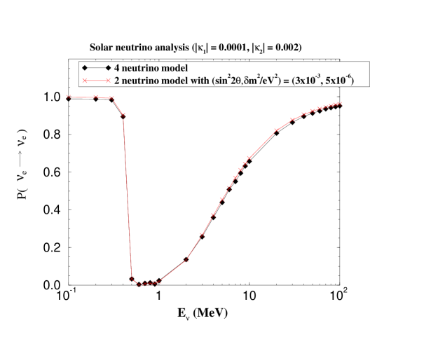
Figure 7 a: Probability $P(\nu_{e}\longrightarrow\nu_{e})$ for solar neutrinos

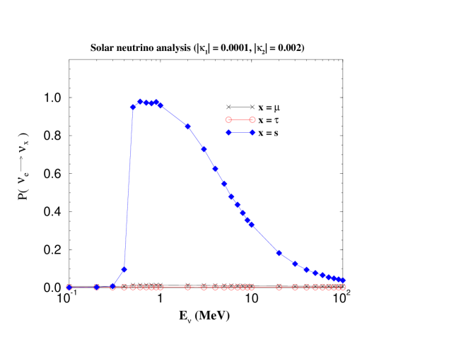
Figure 7 b: Probabilities $P(\nu_{e}\longrightarrow\nu_{x})$ ($x=\mu$, $\tau$ and $s$) for solar neutrinos

Finally with non vanishing $\kappa_{1,2}$ we are now able to simultaneously fit atmospheric, solar and LSND data. This result is shown in figure 8 where we plot the probability $P(\nu_{\mu}\longrightarrow\nu_{e})$ as a function of neutrino energy relevant for LSND for our model compared to a two neutrino model with $sin^{2}2\theta=0.018$ and $\delta m^{2}=0.53$ eV² in the LSND allowed region [3].  This is in contrast to the case $\kappa_{1,2}=0$ (paper I) where this was not possible.

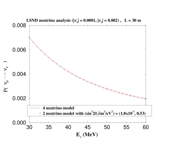
Figure 8: Probability $P(\nu_{\mu}\longrightarrow\nu_{e})$ for LSND energies.

We now consider whether the parameters necessary for the fit make sense. We have three arbitrary parameters. We have taken $b$ and $c$ complex, while any phase for $m^{\prime}$ is unobservable. A large mixing angle for $\nu_{\mu}-\nu_{\tau}$ oscillations is obtained with $|b|\sim 0.05$ [table  14]. This does not require any fine tuning; it is consistent with ${S\ V^{\prime}_{16}\over\phi\ V_{16}}\sim 0.17$ which, taking into account Yukawa couplings, is perfectly natural (see eqn.  54). The parameter $c$ [eqn.  53 and table  14] $\approx 0.10\approx{\mu_{3}\,V_{16}\over\omega\,m_{t}\ \phi}$ implies $\mu_{3}\sim 26(\frac{\phi}{V_{16}})$ GeV. Considering that the standard $\mu$ parameter (see the parameter list in the captions to table 5) with value $\mu=110$ GeV and $\mu_{3}$ [eqn.  26] may have similar origins, both generated once SUSY is spontaneously broken, we feel that it is natural to have a light sterile neutrino. Lastly consider the overall scale of symmetry breaking, i.e. the see-saw scale. We have $m^{\prime}=0.979$ eV [table  14] $\approx{m_{t}^{2}\ \omega\ \phi\over V_{16}\ V^{\prime}_{16}}$. Thus we find ${V_{16}\ V^{\prime}_{16}\over\phi}\sim{m_{t}^{2}\ \omega\over m^{\prime}}\sim 4.66\times 10^{13}$ GeV. This is admittedly somewhat small but perfectly reasonable for $\langle\overline{16}\rangle\sim\langle\phi^{2}\rangle\sim M_{G}$ once the implicit Yukawa couplings are taken into account.

6 Neutrino oscillations [3 active + 2 sterile]

In this case we have $\mu^{\prime}\neq 0,\;\mu_{3}=0$ (see eqn.  30) where $\mu^{\prime}$ sets the scale for the terms $(m_{\nu})_{4\alpha},\;(m_{\nu})_{5\alpha}$ for $\alpha=\{e,\,\mu,\,\tau\}$ (eqn.  57). We are able to find a good solution to atmospheric neutrino oscillations with maximal $\nu_{\mu}\rightarrow\nu_{\tau}$ mixing, a solution to solar neutrino oscillations in the SMA MSW region and a fit to LSND. The fit is presented in tables  16 and  17 and in figures 9(a,b), 10(a,b) and 11.

Note, the parameter $d$ (table  16 and eqn. 57) $=\;\frac{\mu^{\prime}\,V^{\prime}_{16}}{m_{t}\,\phi}$. Thus $\mu^{\prime}=m_{t}\,d\,\frac{\phi}{V^{\prime}_{16}}=0.28\,\frac{\phi}{V^{\prime}_{16}}$ GeV. In addition, we have $m^{\prime}=0.838$ eV [table  16] $\approx{m_{t}^{2}\ \omega\ \phi\over V_{16}\ V^{\prime}_{16}}$. Thus we find $V_{16}\sim{m_{t}^{2}\ \omega\over m^{\prime}}\frac{\phi}{V^{\prime}_{16}}\sim 5.3\times 10^{13}\,\frac{\phi}{V^{\prime}_{16}}$ GeV. In order to obtain this solution without fine tuning we must assume that the ratio $\frac{\phi}{V^{\prime}_{16}}\sim 100$. As in the previous four neutrino case, this may be attributable to ratios of Yukawa couplings.

Table 16: Fit to atmospheric, solar and LSND neutrino oscillations [5 neutrinos   SMA MSW + LSND]
 Initial parameters: $|\kappa_{1}|=|\kappa_{2}|^{2},\;|\kappa_{2}|=0.032$                           $m^{\prime}=0.8380$ eV ,  $b$ = 0.9015,  $d$ = 0.0016,  $\Phi_{b}$ = -3.18rad,  $\Phi_{d}$ = -4.83rad

$$\begin{array}[]{|c|c|}\hline\cr{\rm Observable}&{\rm Computed\;\;value}\\ \hline\cr\delta m^{2}_{atm}&3.7\cdot 10^{-3}\ \rm eV^{2}\\ \sin^{2}2\theta_{atm}&0.99\\ \delta m^{2}_{sol}&5.7\cdot 10^{-6}\ \rm eV^{2}\\ \sin^{2}2\theta_{sol}&4.0\cdot 10^{-3}\\ \delta m^{2}_{LSND}&0.36\\ \sin^{2}2\theta_{LSND}&0.026\\ \hline\cr\end{array}$$

Table 17: Neutrino Masses and Mixings [5 neutrinos   SMA MSW + LSND]
Mass eigenvalues [eV]:    $0.88\cdot 10^{-7}$,  0.0007,  0.0025,  0.6013,   0.6043          
Magnitude of neutrino mixing matrix U_αi                
$i=1,\cdots,5$ – labels mass eigenstates.              
$\alpha=\{e,\ \mu,\ \tau,\ s_{1},\ s_{2}\}$ labels flavor eigenstates.

$$\left[\begin{array}[]{ccccc}0.0586&0.9940&0.0297&0.0763&0.0430\\ 0.0033&0.0802&0.0182&0.6998&0.7096\\ 0.0018&0.0356&0.0617&0.7091&0.7015\\ 0.0036&0.0291&0.9975&0.0401&0.0507\\ 0.9983&0.0585&0.0053&0.0014&0.0015\\ \end{array}\right]$$

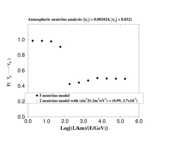
Figure 9 a: Probability $P(\nu_{\mu}\longrightarrow\nu_{\mu})$ for atmospheric neutrinos. For this analysis, we neglect matter effects.

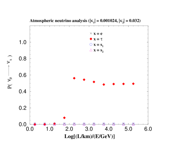
Figure 9 b: Probabilities $P(\nu_{\mu}\longrightarrow\nu_{x})$ ($x=e$, $\tau$, $s_{1}$ and $s_{2}$) for atmospheric neutrinos.

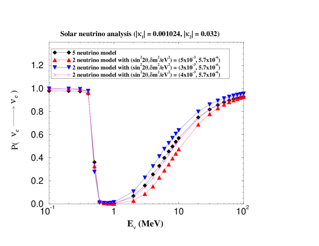
Figure 10 a: Probability $P(\nu_{e}\longrightarrow\nu_{e})$ for solar neutrinos.

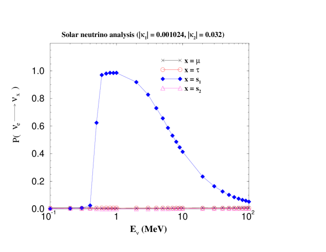
Figure 10 b: Probabilities $P(\nu_{e}\longrightarrow\nu_{x})$ ($x=\mu$, $\tau$, $s_{1}$ and $s_{2}$) for solar neutrinos.

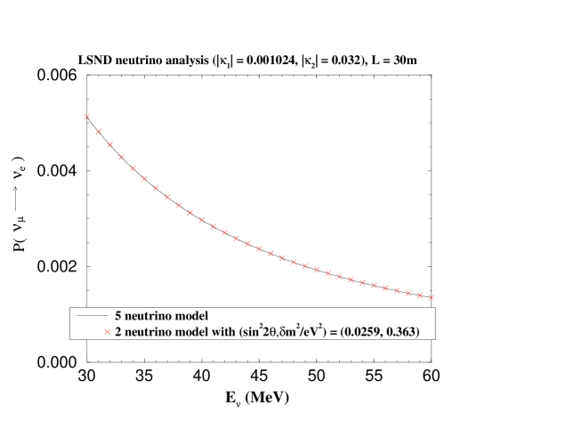
Figure 11: Probability $P(\nu_{\mu}\longrightarrow\nu_{e})$ for LSND energies.

7 Discussion

In this paper we analyze the predictions for both charged fermion and neutrino masses and mixing angles in an SO(10) SUSY GUT with U(2)$\times$U(1)ⁿ family symmetry. We find that, if we allow for the most general family symmetry breaking vevs, the model can accommodate three different three-neutrino oscillation solutions to atmospheric and solar neutrino data, one four and one five neutrino solution to atmospheric, solar and LSND data. We also find a three neutrino solution to atmospheric and LSND data alone. In spite of all this freedom in the neutrino sector, the fits for charged fermion masses and mixing angles are relatively unaffected.

In all cases we find atmospheric neutrino data described by maximal $\nu_{\mu}\rightarrow\nu_{\tau}$ mixing. Super-Kamiokande is able to distinguish $\nu_{\mu}\rightarrow\nu_{x}$ for $\nu_{x}=\nu_{\tau}$ or $\nu_{s}$ (see talks by K. Scholberg and W.A. Mann [2]). There are two proposed methods. The first uses the measured zenith angle dependence, since there is an MSW effect in the earth for $\nu_{s}$ but not for $\nu_{\tau}$. This effect suppresses $\nu_{\mu}\rightarrow\nu_{s}$ oscillations for high energy neutrinos coming from below. Recent data does not show such an effect; thus favoring $\nu_{x}=\nu_{\tau}$. The second method uses the ratio of neutral current [NC] to charged current [CC] processes which can distinguish between the two. Here there is preliminary data favoring $\nu_{x}=\nu_{\tau}$. This ratio satisfies

$$R_{(NC/CC)} <1 \;\;\rm for\;\nu_{x}=\nu_{s}$$

$$=1 \;\;\rm for\;\nu_{x}=\nu_{\tau}.$$

Using SuperK data for $\pi^{0}$ events produced by neutral current neutrino scattering in the detector one measures

$$R_{(NC/CC)} \equiv\frac{(\pi^{0}/e)_{Data}}{(\pi^{0}/e)_{MonteCarlo}}$$

$$=1.11\pm 0.06({\rm data\;stat.})\pm 0.02({\rm MC\;stat.})\pm 0.26({\rm sys.})$$

The oscillations $\nu_{\mu}\rightarrow\nu_{\tau}$ may also be visible at long baseline neutrino experiments. Both K2K  [10] and MINOS  [11] are designed to test for $\nu_{\mu}$ disappearance. For example at K2K [10], the mean neutrino energy $E=1.4$GeV and distance $L=250$ km corresponds to a value of x = 2.3 (see figures 2a, 4a, 6a and 9a) and hence $P(\nu_{\mu}\rightarrow\nu_{\mu})\sim.45$.

Results on solar neutrino oscillations or LSND will, on the other hand, be able to narrow down the acceptable regions of parameter space, but cannot test this class of models.

Finally, the plethora of solutions presented in this paper is in stark contrast to the unique solution obtained assuming the minimal family symmetry breaking vevs studied previously in paper I  [14]. In the latter case we cannot find any three family solutions to both atmospheric and solar data and we find a unique four neutrino solution to atmospheric and solar data but NOT LSND. Thus it is clear that the neutrino sector is in general much less constrained than charged fermions. Nevertheless, it is pleasing to find a simple SUSY GUT which can accommodate all of this low energy data.

Acknowledgements This work is partially supported by DOE grant DOE/ER/01545-767.

8 Appendix

Solar neutrino analysis

In this appendix we describe in detail the approximation which we used in the numerical analysis of solar neutrino oscillations. The Schrödinger equation for solar neutrinos is given by

$$i\frac{d}{dt}\Psi_{\nu}^{\alpha}(t) = H_{\alpha\beta}\Psi_{\nu}^{\beta}(t),$$ (75)

$$H_{\alpha\beta} = \frac{(m_{\nu}^{\dagger}m_{\nu})_{\alpha\beta}}{2E}+V_{\alpha}(t)\delta_{\alpha\beta}.$$ (76)

Here $\Psi_{\nu}^{\alpha}$ is a state vector for neutrinos with flavor $\alpha$ ($\alpha=e$, $\mu$, $\tau$, and $s$ for four neutrino model ), $H$ is the Hamiltonian for solar neutrinos, and $E$ is the neutrino energy. The mass matrix $m_{\nu}$ in the flavor basis is given by (see equation  51)

$$m_{\nu}^{diag}= U^{T}m_{\nu}U$$ , (77)

where $U$ is the mixing matrix for neutrinos ($\nu^{\rm flavor}_{\alpha}=U_{\alpha i}\;\nu^{\rm mass}_{i}$ where $i=1-4$ for four neutrino model) and $m_{\nu}^{diag}$ is the diagonal mass matrix in the mass eigenstate basis. $V_{\alpha}$(t) is a time-dependent potential for neutrinos with flavor $\alpha$ as follows:

$$V_{e}(t) = \sqrt{2}G_{F}\{n_{e}(t)-\frac{1}{2}n_{n}(t)\},$$

$$V_{\mu}(t) = V_{\tau}(t)=-\sqrt{2}G_{F}\frac{1}{2}n_{n}(t),$$

$$V_{s}(t) = 0,$$ (78)

where $G_{F}$ is the Fermi coupling constant. Here we assume that electron ($n_{e}$) and neutron ($n_{n}$) number densities at a distance $r=ct$ from the center of the sun are given by

$$n_{e} = 4.6\times 10^{11}\exp\left(-10.5\frac{r}{R}\right)~{}{\rm eV}^{3},$$ (79)

$$n_{n} = 2.2\times 10^{11}\exp\left(-10.5\frac{r}{R}\right)~{}{\rm eV}^{3},$$ (80)

where $R$ is a solar radius.

Mass scales for the atmospheric and LSND neutrino problems ($\delta m^{2}_{\rm atm.}\simeq 10^{-3}$ eV², $\delta m^{2}_{\rm LSND}\simeq 1$ eV²) are much larger that for the solar neutrino problem ($\delta m^{2}_{\rm solar}\leq 10^{-5}$ eV²). When we include the mass scales for atmospheric and/or LSND neutrinos and solve the Schrödinger equation for the solar neutrino problem, it is almost impossible to solve it numerically because of these larger mass scales and the rapid fluctuations they produce. Thus, in order to solve the Schrödinger equation numerically, we use the following approximation.

We divide the mass term $m_{\nu}^{\dagger}m_{\nu}$ into two parts:

$$m_{\nu}^{\dagger}m_{\nu} = U\;(m_{\nu}^{diag})^{\dagger}m_{\nu}^{diag}\;U^{\dagger},$$ (81)

$$= U\;m_{L}^{2}\;U^{\dagger}+U\;m_{H}^{2}\;U^{\dagger},$$

where $m_{L}^{2}$ ($m_{H}^{2}$) is a “Light” (“Heavy”) part,

$$m^{2}_{L} = \left(\begin{array}[]{cccc}m_{1}^{2}&&&\\ &m_{2}^{2}&&\\ &&0&\\ &&&0\\ \end{array}\right),$$ (86)

$$m_{H}^{2} = \left(\begin{array}[]{cccc}0&&&\\ &0&&\\ &&m_{3}^{2}&\\ &&&m_{4}^{2}\\ \end{array}\right),$$ (91)

and we assume that $\delta m^{2}_{21}=m^{2}_{2}-m^{2}_{1}$ is the scale for solar neutrino problem and $m_{1}^{2}<m_{2}^{2}\ll m_{3}^{2}<m_{4}^{2}$. Then the Hamiltonian $H$ is given as

$$H = H_{H}+H_{L},$$

$$H_{H} = U\frac{m_{H}^{2}}{2E}U^{\dagger},$$ (92)

$$H_{L} = U\frac{m_{L}^{2}}{2E}U^{\dagger}+V_{\alpha}(t)\delta_{\alpha\beta}.$$ (93)

The state vector is also divided into two parts as follows:

$$\Psi_{\nu}^{\alpha}(t)=A_{\alpha\beta}(t)\;\Phi_{\nu}^{\beta}(t),$$ (94)

where we define $A$ to satisfy the following equation:

$$i\frac{d}{dt}A(t) = H_{H}A(t),$$

$$A(t=0) = I$$ (95)

where $I$ is a unit matrix. We can easily solve the equation ( 95) and the solution is given by

$$A(t) = \exp(-iH_{H}t),$$ (96)

$$= U\exp\left(-i\frac{m_{H}^{2}}{2E}t\right)U^{\dagger}.$$

Then $\Phi_{\nu}$ satisfies

$$i\frac{d}{dt}\Phi_{\nu}(t)=U\left[\frac{m_{L}^{2}}{2E}+\exp\left(i\frac{m_{H}^{2}}{2E}t\right)U^{\dagger}V(t)U\exp\left(-i\frac{m_{H}^{2}}{2E}t\right)\right]U^{\dagger}\Phi_{\nu}(t).$$ (97)

Since the mass scales $m_{3,4}$ included in the matrix $m_{H}^{2}$ are too large for MSW effects, the exponential terms $\exp\left(\pm i\frac{m_{3,4}^{2}}{2E}t\right)$ oscillate rapidly. Therefore we replace them by their time-averaged values:

$$\exp\left(\pm i\frac{m_{3,4}^{2}}{2E}t\right) \rightarrow 0$$ (98)

Then equation 97 has the following approximate form

$$i\frac{d}{dt}\Phi_{\nu}^{\alpha}(t) \simeq \left[U_{\alpha i}\left(\frac{m^{2}_{Li}}{2E}\delta_{ij}+U^{\dagger}_{i\gamma}V_{\gamma}(t)U_{\gamma j}\right)U^{\dagger}_{j\beta}\right.$$ (99)

$$\left.+U_{\alpha~{}i+2}U^{\dagger}_{i+2~{}\gamma}V_{\gamma}(t)U_{\gamma~{}i+2}U^{\dagger}_{i+2~{}\beta}\right]\Phi_{\nu}^{\beta}(t),$$

where the indices $\alpha,~{}\beta,~{}\gamma$ run from 1 to 4, on the other hand, the indices $i,~{}j$ from 1 to 2. We then solve equation  99 with the initial condition

$$\Phi_{\nu}(t=0)=(1,0,0,0)~{}~{}~{}{\rm or}~{}~{}~{}\Psi_{\nu}(t=0)=(1,0,0,0).$$ (100)

Finally, the oscillation probability $P(\nu_{e}\rightarrow\nu_{\alpha})$ ($\alpha=e,\mu,\tau$ or $s$) at time $t$ is given by

$$P(\nu_{e}\rightarrow\nu_{\alpha}) = \left|\Psi_{\nu}^{\alpha}(t)\right|^{2}$$ (101)

$$= \left|A_{\alpha\beta}(t)\;\Phi_{\nu}^{\beta}(t)\right|^{2}$$

$$\simeq \left|\sum_{i=1,2,\beta=1-4}U_{\alpha i}\ U^{\dagger}_{i\beta}\ \Phi_{\nu}^{\beta}\right|^{2}+\sum_{i=3,4}\left|\sum_{\beta=1-4}U_{\alpha i}\ U^{\dagger}_{i\beta}\ \Phi_{\nu}^{\beta}\right|^{2}.$$

where the $\simeq$ in the last line (equation 101) refers to the fact that the time average of $\exp(\pm i\frac{m_{3,4}^{2}}{2E}t)$ was used.

References

[1] For results from the Homestake experiment, see B.T. Cleveland et al., Astrophys. J.496, 505 (1998), B.T. Cleveland et al., Nucl. Phys.B38(Proc. Supp.), 47 (1995); from SAGE, see V. Gavrin et al., in Neutrino 96, Proceedings of the XVII International Conference on Neutrino Physics and Astrophysics, Helsinki, edited by K. Huitu, K. Enquist and J. Maalampi (World Publishing, Singapore, 1997), p. 14; from GALLEX, see GALLEX Collaboration, P. Anselmann et al., Phys. Lett.B342, 440 (1995). For results from Kamiokande, see KAMIOKANDE Collaboration, Y. Fukuda et al., Phys. Rev. Lett.77, 1683 (1996); and from Super-Kamiokande, see Y. Fukuda et al., Phys. Rev. Lett. (1998), hep-ex/9805021. For recent results from Super-Kamiokande, see talk by M. Smy,
DPF99, UCLA, hep-ex/9903034.
[2] The Super-Kamiokande Collaboration, Phys. Rev. Lett.81 1562 (1998). For a more recent analysis, see K. Scholberg, Talk presented at 8th International Workshop on Neutrino Telescopes, Venice, February 23-26 1999, hep-ex/9905016 and W.A. Mann, Talk presented at the XIX International Symposium on Lepton and Photon Interactions at High Energies,
Stanford University, August 9-14, 1999, hep-ex/9912007.
[3] LSND Collaboration, C. Athanassopoulos et al., Phys. Rev.
Lett.81 1774 (1998); ibid., Phys. Rev.C58 2489 (1998).
[4] CHOOZ Collaboration, M. Apollonio et al., Phys.Lett.B420 397 (1998).
[5] B. Bodmann et al., Phys. Lett.B267, 321 (1991);
B. Bodmann et al., Phys. Lett.B280, 198 (1992); B. Zeitnitz et al., Prog. Part. Nucl. Phys.32, 351 (1994); K. Eitel, hep-ex/9706023.
[6] J.N. Bahcall, P.I. Krastev and A. Yu.
Smirnov, Phys. Rev.D58 096016 (1998) and references therein;
V. Barger, S. Pakvasa, T. J. Weiler, K. Whisnant, Phys. Rev.D58, 093016 (1998); V. Barger, S. Pakvasa, T.J. Weiler, K. Whisnant, Phys. Lett.B437, 107-116 (1998); G. Altarelli and F. Feruglio, Jour. of HEP9811 021 (1998); R. Barbieri, L.J.
Hall, D. Smith, A. Strumia and N. Weiner, hep-ph/9807235; R.N. Mohapatra and
S. Nussinov, hep-ph/9808301 ; V. Barger,hep-ph/9808353; V. Barger and K.
Whisnant, hep-ph/9812273; S.L. Glashow, P.J. Kernan and L.M. Krauss, Phys. Lett.B445 412 (1999); G.L. Fogli, E. Lisi, A. Marrone, G. Scioscia, Phys. Rev.D59, 033001 (1999); G.L. Fogli, E. Lisi, D. Montanino, Phys. Lett.B434, 333-339 (1998); S.M. Bilenky, C. Giunti, W. Grimus, hep-ph/9812360, to be published in Progress in Particle and Nuclear Physics, Volume 43. For recent analyses, see J.N. Bahcall, P.I. Krastev and A. Yu.
Smirnov, hep-ph/9905220 and M.C. Gonzalez-Garcia, P.C. de Hollanda, C. Pena-Garay and J.W.F. Valle, hep-ph/9906469.
[7] See http://www.sno.phy.queens_u.ca/
[8] See http://almime.mi.infn.it/
[9] See http://www.neutrino.lanl.gov/BooNE/; E. Chruch et al., FERMILAB-P-0898 (1997).
[10] Y. Oyama, hep-ex/9803014 (1998).
[11] See http://www.hep.anl.gov/NDK/ HyperText/minos.tdr.html. P875, A Long Baseline Neutrino Oscillation Experiment at Fermilab, February (1995); Dave Ayres for the MINOS collaboration, A Summary of the MINOS proposal, A Long Baseline Neutrino Oscillation Experiment at Fermilab, March (1995); NuMI note: NuMI-L-71, see http://www.hep.anl.gov/NDK/ HyperText/numi_notes.html.
[12] See http://www.aquila.infn.it/icarus.; C. Rubbia et al., LNGS-94/99 Vol. I & II (1994); C. Rubbia, Nucl. Phys. Proc. Suppl.48 172 (1996).
[13] Y.F. Wang, STANFORD-HEP-98-04 (1998); P. Alivisatos et al., STANFORD-HEP-98-03 (1998).
[14] T. Blazek, S. Raby and K. Tobe, Phys. Rev.D60 113001 (1999).
[15] T. Blazek, M. Carena, S. Raby and C. Wagner,
Phys. Rev.D56 6919 (1997).
[16] L. Wolfenstein, Phys. Rev.D17, 2369 (1978); S.P. Mikheyev and A. Yu. Smirnov, [Yad. Fiz.42, 1441 (1985) [Sov. J. Nucl. Phys.42, 913 (1985), Nuovo Cim.C9, 17 (1986).
[17] R. Barbieri, L.J. Hall, S. Raby and A. Romanino, Nucl. Phys.B493 3 (1997); R. Barbieri, L.J. Hall and A. Romanino, Phys. Lett.B401 47 (1997).
[18] L.J. Hall and L. Randall, Phys. Rev.
Lett.65 2939 (1990); M. Dine, R. Leigh and A. Kagan, Phys. Rev.D48 4269 (1993); Y. Nir and N. Seiberg, Phys. Lett.B309 337 (1993); P. Pouliot and N. Seiberg, Phys. Lett.B318 169 (1993); M. Leurer, Y. Nir and N. Seiberg, Nucl. Phys.B398 319 (1993); M. Leurer, Y. Nir and N. Seiberg, Nucl. Phys.B420 468 (1994); D. Kaplan and M. Schmaltz, Phys. Rev.D49 3741 (1994); A. Pomarol and D. Tommasini, Nucl.Phys.B466 3 (1996); L.J. Hall and H. Murayama, Phys. Rev. Lett.75 3985 (1995); P. Frampton and O. Kong, Phys. Rev. Lett.75 781 (1995) and ibid., Phys.Rev.D53 2293 (1996); E. Dudas, S. Pokorski and C.A. Savoy, Phys. Lett.B356 45 (1995) and ibid.,
Phys. Lett.B369 255 (1996); C. Carone, L.J. Hall and H. Murayama, Phys. Rev.D53 6282 (1996); P. Binetruy, S. Lavignac and P. Ramond,
Nucl. Phys.B477 353 (1996); V. Lucas and S. Raby,
Phys. Rev.D54 2261 (1996); Z. Berezhiani, Phys.Lett.B417 287 (1998).
[19] M. Dine, R. Leigh and A. Kagan, Phys. Rev.D48 4269 (1993); A. Pomarol and D. Tommasini, Nucl.Phys.B466 3 (1996); R. Barbieri, G. Dvali and L.J. Hall, Phys. Lett.B377 76 (1996); R. Barbieri and L.J. Hall, Nuovo Cim.110A 1 (1997).
[20] S. Dimopoulos and H. Georgi, Nucl. Phys.B193 150 (1981); L.J. Hall, V.A. Kostelecky and S. Raby, Nucl.
Phys.B267 415 (1986); H. Georgi, Phys.Lett.169B 231
(1986); F. Borzumati and A. Masiero, Phys. Rev. Lett.57 961 (1986);
R. Barbieri and L.J. Hall, Phys. Lett.B338 212 (1994); R. Barbieri, L.J. Hall and A. Strumia, Nucl. Phys.B445 219 (1995); J. Hisano, T. Moroi, K. Tobe, M. Yamaguchi and T. Yanagida, Phys. Lett.B357 579 (1995); F. Gabbiani, E. Gabrielli, A. Masiero and L. Silvestrini, Nucl.
Phys.B477 321 (1996); S. Dimopoulos and A. Pomarol, Phys.
Lett.B353 222 (1995); J. Hisano, T. Moroi, K. Tobe and M. Yamaguchi, Phys. Rev.D53 2442 (1996); ibid., Phys. Lett.B391 341
(1997); K. Tobe, Nucl. Phys. (Proc. Suppl.) B59, 223
(1997); J. Hisano, D. Nomura, T. Yanagida, Phys. Lett.B437 351
(1998); J. Hisano, D. Nomura, Y. Okada, Y. Shimizu, M. Tanaka, Phys. Rev.D58 116010 (1998); J. Hisano and D. Nomura, hep-ph/9810479.
[21] C. Froggatt and H.B. Nielsen, Nucl. Phys.B147 277
(1979).
[22] P. Langacker, talk presented at the 17th International Workshop on Weak Interactions and Neutrinos, Cape Town, January 24 - 30, 1999,
hep-ph/9905428; and talk presented at the Greater Chicagoland Seminar, Chicago, October 18, 1999 (unpublished).
[23] R. Gupta, D. Daniel, G.W. Kilcup, A. Patel and S.R. Sharpe,
Phys. Rev.D47, 5113 (1993); G. Kilcup, Phys. Rev. Lett.71, 1677 (1993); S. Sharpe, Nucl. Phys. B (Proc. Suppl.) 34, 403 (1994).
The same mean value and standard deviation for were given in a recent
review article: U.Nierste,”Phenomenology of in the Top Era”,
invited talk at the workshop on K physics, Orsay, France, May 30 - June 4, 1996
(LANL hep-ph/9609310).
[24] T. Blazek, R. Dermisek, A. Mafi, S. Raby and K. Tobe, in progress.
[25] David Hertzog, Precision Measurement of the Muon’s Anomalous Magnetic Moment and the Standard Model, colloquium talk at Northwestern Univ., November 10, 1999. Hertzog quoted with the current world average with the preliminary BNL result included.
[26] M. Gell-Mann, P. Ramond and R. Slansky, in Supergravity, ed.
P. van Nieuwenhuizen and D.Z. Freedman, North-Holland, Amsterdam, 1979, p. 315
; T. Yanagida, in Proceedings of the Workshop on the unified theory and the
baryon number of the universe, ed. O. Sawada and A. Sugamoto, KEK report No.
79-18, Tsukuba, Japan, 1979.
[27] C.D. Carone and L.J. Hall, Phys.Rev.D56 4198
(1997); L.J. Hall and N. Weiner, hep-ph/9811299.
[28] R.N. Mohapatra and J.W.F. Valle, Phys. Rev.D34
1634 (1986).
[29] O.L.G. Peres and A. Yu. Smirnov, “Testing the Solar Neutrino Conversion with Atmospheric Neutrinos,” hep-ph/9902312 (1999).
[30] V. Barger, S. Pakvasa, T.J. Weiler, K. Whisnant, Phys. Lett.B437, 107 (1998).
[31] see also, V. Barger and K. Whisnant, Phys. Rev.D59 093007 (1999) (hep-ph/9812273).