Sensitivity plots for WIMP direct detection using the annual modulation signature

Abstract

Annual modulation due to the Earth’s motion around the Sun is a well known signature of the expected WIMP signal induced in a solid state underground detector. In the present letter we discuss the prospects of this technique on statistical grounds, introducing annual-modulation sensitivity plots for the WIMP–nucleon scalar cross section for different materials and experimental conditions. The highest sensitivity to modulation is found in the WIMP mass interval $10\;{\rm GeV}\mathrel{\mathop{\kern 0.0pt\hbox to0.0pt{\raise 0.86108pt\hbox{$<$}\hss}}\lower 3.87495pt\hbox{\kern-1.90002pt$\sim$}}m_{W}\mathrel{\mathop{\kern 0.0pt\hbox to0.0pt{\raise 0.86108pt\hbox{$<$}\hss}}\lower 3.87495pt\hbox{\kern-1.90002pt$\sim$}}130\;{\rm GeV}$, the actual upper limit depending from the choice of the astrophysical parameters, while the lowest values of the explorable WIMP–nucleon elastic cross-sections fall in most cases within one order of magnitude of the sensitivities of present direct detection WIMP searches.

I Introduction

Non barionic Cold Dark Matter is a basic component in cosmological models of structure formation. Taking into account the result of microlensing surveys, it can be stated that dark baryons can account for at most only about one-third of the estimated density of our dark halo. The best candidates to provide the rest are Weakly Interacting Massive Particles (WIMP), among which the neutralino, provided by the Supersymmetric extension of the Standard Model, is one of the favourites.

It is well known that all WIMP direct searches, which look for the WIMP elastic scattering off the nuclei of a suitable detector, are essentially constrained by the fact that the predicted differential rate of the signal has a dependence with decreasing energy which is hardly distinguishable from the background recorded in the detector. While this fact does not prevent us in extracting upper bounds of the WIMP–nucleus interaction cross–section for each WIMP mass, a distinctive signature is needed to claim a positive identification of the WIMP. In any case, the non appearance of the genuine signature looked for could provide a background–rejection method useful to improve the experimental sensitivity.

The only identification signatures of the WIMP explored up to now are provided by the features of the Earth’s motion with respect to the Dark Matter halo. In particular the annual modulation effect[1] is provided by the combination of the motion of the solar system in the Galactic rest frame and the rotation of the earth around the Sun. Due to this effect the incoming WIMP’s velocities in the detector rest frame change continuously during the year, having a maximum in summer and a minimum in winter.

Several experiments have already searched for this effect[2, 3, 4] one of which[5] reports a possible positive signal. The present situation is no doubt exciting, since experimental sensitivities of underground detectors are entering for the first time the supersymmetric parameter space, and a host of new experiments will soon start to probe it with even higher sensitivity. In the present paper we discuss on purely statistical grounds the perspectives of modulation searches taking into account the features of present and future experiments. Sensitivity plots will be introduced in order to convey in a compact way all the necessary information.

II Extracting the modulation signal

The procedure to extract a modulated signal with a given period and phase from a set of measured count rates has been discussed by several authors[6, 7, 8, 5].

Due to the Earth’s rotation around the Sun, the expected count rate of WIMP’s scatterings off the target’s nucleus changes periodically in time. The dependence may be approximated by a cosine function with period T=1 year and phase $t_{0}=2^{nd}$ june:

$$S=S_{0}+S_{m}\cos\omega(t_{i}-t_{0})$$ (1)

where $S_{0}$ and $S_{m}$ are the constant and the modulated amplitude of the signal respectively. The oscillating frequency is $\omega=2\pi/T$ and the $i$ index indicates the day. The theoretical inputs introduced in the evaluation of the WIMP-nucleus elastic scattering (cross sections, nuclear form factors, scalar, vectorial or spin–dependent nature of the coupling) and all the parameters entering in the halo velocity distribution (r.m.s. and escape WIMP velocity, local dark matter density) make the evaluation of the functions $S_{0}$ and $S_{m}$ rather model dependent [9]. As is costumary, the amplitudes $S_{0}$ and $S_{m}$ are expressed in terms of the WIMP mass $m_{W}$ and of the point–like WIMP–nucleus cross section $\sigma$.

Given a set of experimental count rates $N_{ik}$ representing the number of events collected in the i-th day and k-th energy bin (the formalism can be easily generalized to the case of a multiple-crystal set-up), the mean value of $N_{ik}$ is:

$$<N_{ik}>\equiv\mu_{ik}=\left[b_{k}+S_{0,k}+S_{m,k}\cos\omega(t_{i}-t_{0})\right]\cdot W_{ik}$$ (2)

where the $b_{k}$ and the $S_{ik}\equiv S_{0,k}+S_{m,k}\cos\omega(t_{i}-t_{0})$ represent the average background and the signal respectively, in number of counts per unit of detector mass, time and interval of collected energy $E$ (which is related to the recoil energy $E_{R}$ by the relation $E=QE_{R}$ where $Q$ is the quenching factor of the detector). $W_{ik}=M\Delta T_{i}\Delta E_{k}\epsilon_{k}$ are the corresponding exposures, where $M$ is the mass of the detector, $\Delta E_{k}$ is the amplitude of the k-th energy–bin, while $\Delta T_{i}$ represents the i-th time bin (in the following we will assume all $\Delta T_{i}$= 1 day). The $\epsilon_{k}$ are efficiencies that have to be taken into account whenever some subtraction method is used with the data. In the following they will be neglected. For simplicity also $t_{0}$ will be omitted in the following equations.

A general procedure to compare theory with experiment is to use the maximum-likelihood method. The combined-probability function of all the collected $N_{ik}$, assuming that they have a poissonian distribution with mean values $\mu_{ik}$, is given by:

$$L=\prod_{ik}e^{-\mu_{ik}}\frac{\mu_{ik}^{N_{ik}}}{N_{ik}!}.$$ (3)

Assuming that the average background rates $b_{k}$ and the efficiencies $\epsilon_{k}$ are constant in time, a possible WIMP oscillating solution can be searched for in the data. This implies that the time–dependent fluctuations of background and efficiencies should stand well below the size of the searched modulation effect, if one wishes to disregard any other less exotic explanation of a modulation of the data. If this condition is verified, a WIMP analysis is justified, and the most probable values of $m_{W}$ and $\sigma$ maximize $L$ or, equivalently, minimize the function:

$$y(m_{W},\sigma) \equiv -2\log{L}-const$$ (4)

$$= 2\mu-2\sum_{ik}N_{ik}\log\left[b_{k}+S_{0,k}+S_{m,k}\cos\omega t_{i}\right]$$ (5)

where $\mu\equiv\sum_{ik}\mu_{ik}$ and all the parts not depending on $m_{W}$ and $\sigma$ may be absorbed in the constant because are irrelevant for the minimization.

The function $y$ is minimized in a two–step procedure, first with respect to the time–independent parts $f_{k}\equiv b_{k}+S_{0,k}$ and then with respect to $m_{W}$ and $\sigma$. In the first minimization the $b_{k}$ are free parameters with the only constraint to be positive. So the condition $S_{0,k}\leq f_{jk,min}$, or otherwise $S_{0,k}$=$f_{jk,min}$, is imposed.

Following a standard procedure[10], a region of n standard deviations around the minimum in the plane $(\sigma,m_{W})$ can be found by imposing the condition $y(\sigma,m_{W})-y_{min}\leq n^{2}$.

III Data reduction

Although the likelihood function $L$ depends on all the collected data $N_{ik}$, only suitable combinations of the $N_{ik}$ enter in the determination of the parameters $\sigma$ and $m_{W}$. By expanding $y$ in powers of $x_{k}\equiv S_{m,k}/f_{k}\mathrel{\mathop{\kern 0.0pt\hbox to0.0pt{\raise 0.86108pt\hbox{$<$}\hss}}\lower 3.87495pt\hbox{\kern-1.90002pt$\sim$}}$ few % up to terms of the order $x_{k}^{2}$ the following expression can be obtained (here and in the following $Var$ indicates the variance):

$$y(\sigma,m_{W}) = \sum_{k}\frac{(S_{m,k}(\sigma,m_{W})-X^{\prime}_{k})^{2}}{Var(X^{\prime}_{k})}+{\cal O}(x_{k}^{3})+F(N_{ik})$$ (6)

$$X^{\prime}_{k} \equiv \frac{\sum_{i}N_{ik}\cos{\omega t_{i}}-N_{k}\beta_{k}}{W_{k}(\hat{\alpha}_{k}-\hat{\beta}_{k}^{2})}\;\;\;\;Var(X_{k}^{\prime})\equiv\frac{N_{k}}{W_{k}^{2}(\hat{\alpha}_{k}-\hat{\beta}_{k}^{2})}$$ (7)

where $\beta_{k}\equiv\frac{\sum_{i}W_{ik}cos\omega t_{i}}{W_{k}}$, $\hat{\alpha}_{k}\equiv\frac{\sum_{i}N_{ik}cos^{2}\omega t_{i}}{N_{k}}$, $\hat{\beta}_{k}\equiv\frac{\sum_{i}N_{ik}cos\omega t_{i}}{N_{k}}$, $N_{k}\equiv\sum_{i}N_{ik}$, $W_{k}\equiv\sum_{i}W_{ik}$. The last term of Eq.(6) may be dropped, since it does not depend on the fitting parameters. This implies that the likelihood function has an approximate factorization $L\simeq F_{1}(N_{ik})\cdot F_{2}(X_{k}^{\prime},\sigma,m_{W})$ and the information to determine $\sigma$ and $m_{W}$ is only contained in the $X^{\prime}_{k}$ up to negligible corrections. As expected on general grounds, Eq.(6) reduces asymptotically to a $\chi^{2}$: this happens when the $X_{k}^{\prime}$’s have gaussian distributions (in the examples that will be discussed in the following we have checked that this is always verified).

The expressions (7) of the $X_{k}^{\prime}$ s are asymptotically equal to the cosine projections introduced in ref. [6] (generalized to the case of discontinuous data taking and unpaired days) to extract a modulated signal,

$$X_{k} \equiv \frac{\sum_{i}N_{ik}\cos{\omega t_{i}}-N_{k}\beta_{k}}{W_{k}(\alpha_{k}-\beta_{k}^{2})}\;\;;<X_{k}>=S_{m,k}$$ (8)

$$Var(X_{k}) \equiv \frac{\sum N_{ik}cos^{2}\omega t_{i}+\beta_{k}^{2}N_{k}-2\beta_{k}\sum N_{ik}\cos\omega t_{i}}{W_{k}^{2}(\alpha_{k}-\beta_{k}^{2})^{2}}$$ (9)

with $\alpha_{k}\equiv\frac{\sum_{i}W_{ik}cos^{2}\omega t_{i}}{W_{k}}$. (For the sake of comparison with Eq.(7) it is convenient to use the identity $N_{k}\equiv(\sum N_{ik}\cos^{2}\omega t_{i}+\hat{\beta}_{k}^{2}N_{k}-2\hat{\beta}_{k}\sum N_{ik}\cos\omega t_{i})/(\hat{\alpha}_{k}-\hat{\beta}_{k}^{2})$ in the expression of $Var(X^{\prime}_{k})$). This implies that the likelihood function $y$ has also the asymptotic behaviour:

$$y(\sigma,m_{W})=\chi^{2}(\sigma,m_{W})\;\;\;;\chi^{2}(\sigma,m_{W})\equiv\sum_{k}\frac{(S_{m,k}(\sigma,m_{W})-X_{k})^{2}}{Var(X_{k})}.$$ (11)

In the case of paired days ($\beta_{k}=0$) and if only time intervals close to the maximum and the minimum of the cosine function are considered ($\cos\omega t_{i}\simeq\pm 1$) the $X_{k}$’s reduce to the june–december differences in the collected count rates in each energy bin $E_{k}<E<E_{k}+\Delta E_{k}$.

IV Statistical significance of the signal

Once a minimum of the likelihood function is found, a positive result excludes absence of modulation at some confidence level probability. This can be checked by evaluating the quantity $\delta^{2}=y(\sigma=0)-y(\sigma,m_{W})_{min}$ to test the goodness of the null hypothesis. In order to study the distribution of $\delta^{2}$ we make use of the asymptotic behaviour (11). This implies:

$$\delta^{2}=y(\sigma=0)-y_{min}\simeq\chi^{2}(\sigma=0)-\chi^{2}_{min}.$$ (12)

In the case of absence of a modulation effect (i.e. time-independent Poisson-fluctuating data) numerical simulations show that the quantity $\delta^{2}$ belongs asymptotically to a $\chi^{2}$ distribution with two degrees of freedom. We explain this by the fact that once the cross section $\sigma$ is set to zero the likelihood function $L$ no longer depends on $m_{W}$ (all the $S_{0}$ and $S_{m}$ functions vanish) and this is equivalent to fixing both the parameters of the fit at the same time.

In presence of the signal the minimization procedure of $y$ described in the previous section may be carried out semi–analytically using Eq.(11). One finds for $\sigma$ the estimator $\sigma_{est}$ given by:

$$\sigma_{est} = \frac{\sum_{k}\frac{X_{k}\hat{S}_{m,k}(m_{W}^{0})}{Var(X_{k})}}{\sum_{k}\frac{\hat{S}_{m,k}(m_{W}^{0})^{2}}{Var(X_{k})}}$$ (13)

$$Var(\sigma_{est}) = \left(\sum_{k}\frac{\hat{S}_{m,k}(m_{W}^{0})^{2}}{Var(X_{k})}\right)^{-1}.$$ (14)

$\sigma_{\rm est}$ is a function of the data, such that $<\sigma_{\rm est}>=\sigma$ (where brackets indicate mean value). In Eqs.(13,14) $\hat{S}_{m,k}(m_{W})\equiv S_{m,k}(\sigma,m_{W})/\sigma$ and $m_{W}^{0}$ is the WIMP mass that maximizes the function $\delta(m_{W})$, which is given by:

$$\delta(m_{W})=\frac{\sum_{k}\frac{X_{k}\hat{S}_{m,k}(m_{W})}{Var(X_{k})}}{\sqrt{\sum_{k}\frac{\hat{S}_{m,k}(m_{W})^{2}}{Var(X_{k})}}}=\frac{\sigma_{est}}{\sqrt{Var(\sigma_{est})}}.$$ (15)

From equation (15) $\delta\equiv\delta(m_{W}^{0})$ may be interpreted, as expected, as the number of standard deviations of the signal, with:

$$Var(\delta) = 1;$$ (16)

$$<\delta>=<\frac{\sigma_{est}}{\sqrt{Var(\sigma_{est})}}> = \sqrt{<\delta^{2}>-1}$$ (17)

so in presence of modulation $\delta^{2}$ has the asymptotic distribution of a non central $\chi^{2}$ with one degree of freedom and non centrality parameter given by $(<\sigma_{\rm est}/\sqrt{Var(\sigma_{est})}>)^{2}=$$<\delta^{2}>-1$.

Using Eqs.(11,12) we obtain:

$$<\delta^{2}>=\frac{1}{2}\sum_{k}\frac{S_{m,k}(\sigma,m_{W})^{2}\Delta E_{k}}{b_{k}+S_{0,k}}MT\alpha+2.$$ (18)

where the same days of data taking have been assumed for all the energy bins, and in the expression of $Var(X_{k})$ the following approximations have been made:

$$<\sum_{i}N_{ik}\cos^{2}\omega t_{i}> \simeq <N_{ik}>\sum_{i}\cos^{2}\omega t_{i}$$ (19)

$$<N_{ik}> \simeq W_{k}(b_{k}+S_{0})$$ (20)

while we define the factor of merit $\alpha\equiv\frac{2}{T}\sum_{i}\cos^{2}\omega t_{i}$ ($\alpha$=1 in case of a full period of data taking) and the terms depending on the $\beta_{k}$ have been neglected.

Equation (18) allows to estimate the needed exposure MT$\alpha$ in order to obtain a given value of $<\delta^{2}>$. (It is worth noticing that the background $b_{k}$ indicates here the amount of counts expected from radioactive contamination and noise, for instance evaluated by making use of a Montecarlo simulation, and not the average counts, that contain also the signal). Whenever the distribution of $\delta^{2}$ for a given WIMP model is sufficiently far apart from that of the background, a given experimental result may be discriminated to belong to one population or the other. Once a required $<\delta^{2}>$ is chosen, a sensitivity plot may be obtained by showing the curves of constant MT$\alpha$ in the plane $m_{W}$–$\sigma$.

The statistical interpretation of the sensitivity plot is obtained from the degree of overlapping between the distributions of $\delta^{2}$ in the two cases of absence and presence of modulation. The situation is summarized in Table I, where $<\delta^{2}>$ is tabulated as a function of the fraction of experiments where absence of modulation can be excluded (rows), and the required Confidence Level (columns). For instance, if $<\delta^{2}>$=14.9, there is a 90% probability to measure a value of $\delta^{2}$ higher than 7: this range would exclude the absence of modulation at least at the 95 % C.L. In the same way a less demanding value of $<\delta^{2}>$=5.6 would give a 50% probability to see an effect at the 90% C.L. or more. In the following section, we will adopt these two representative values in order to discuss the prospects of modulation searches. This procedure allows to see in a compact way the masses and exposures needed to explore each different region of the WIMP $m_{W}$–$\sigma$ parameter space.

The expression of $<\delta^{2}>$ in Eq.(18) deserves a short comment. Some attention has been devoted in discussions on the perspectives of modulation searches[8, 7] to the fact that since the $S_{m,k}$ parameters can vanish or be negative, cancellations may arise in the calculation of the signal–to–noise ratio, so that an optimal choice should be found for the energy threshold or for the amplitude of the energy interval where the signal is integrated. According to Eq.(18), in order to exploit all the information available, the signal–to–noise ratio should be calculated over the whole energy spectrum, using the smallest bin width allowed by statistics and resolution, and then combined quadratically, i.e.:

$$({\rm signal/noise})^{2}_{{\rm combined}}=\sum_{i}({\rm signal/noise})^{2}_{i}$$ (21)

where $i$ indicates the energy bin. Of course in this procedure it is crucial that the count rates of different bins are not correlated.

V Sensitivity plots and quantitative discussion

In this section we give a quantitative discussion of the sensitivity plots by considering different target materials: $Ge$, $TeO_{2}$, $NaI$ with quenching factors, experimental thresholds and resolutions summarized in Table II (they have been chosen in order to be indicative of running or planned experiments[5, 11, 12, 13, 14]). For simplicity, in order to calculate the sensitivity plots, a flat background will be always assumed and in the following the index $k$ of $b_{k}$ will be dropped.

As far as the astrophysical parameters entering in the calculation are concerned, we assume as usual that the WIMP velocities in the halo follow a Maxwellian distribution. The WIMP r.m.s. velocity $v_{\rm rms}$ is related to the measured rotational velocity of the Local System at the Earth’s position $v_{\rm loc}$ by the relation $v_{\rm rms}^{2}=\frac{2}{3}\;v_{\rm loc}^{2}$, while the Sun’s velocity $v_{\rm sun}$ in the galactic rest frame is given by $v_{\rm sun}\simeq(v_{\rm loc}+12)$ km sec^-1 (here the motion of the solar system with respect to the Local System is taken into account) and the Earth velocity is:

$$v_{\rm earth}=v_{\rm sun}+v_{\rm orb}\sin\delta\cos\left[\omega(t-t_{0})\right]$$ (22)

where $v_{orb}\simeq$ 30 km sec^-1 and $\sin\delta\simeq$ 0.51[6] ($\delta$ is the angle between the Ecliptic and the Galactic plane).

As it has been pointed out in the literature[15] the present uncertainty on $v_{\rm loc}$ can affect the final result of WIMP direct detection calculations in a significant way. In the following we will vary $v_{\rm loc}$ in its physical range, $v_{\rm loc}=(220\pm 50)$ km sec^-1. Finally, we adopt an escape velocity $v_{\rm esc}$=650 km/sec and take for the local halo mass density the value $\rho$=0.3 GeV/cm³.

In order to compare the results for different target materials in the same plots, we show our results in the plane $m_{W}-\sigma^{(n)}$, where $\sigma^{(n)}$ is the WIMP cross section rescaled to the nucleon by adopting a scalar–type interaction (such as the one that would be dominant in the case of a neutralino). In the case of a monoatomic target this implies the transformation:

$$\sigma=\sigma^{(n)}A^{2}\frac{\mu^{2}_{W,N}}{\mu^{2}_{W,n}}$$ (23)

where $A$ is the target atomic number, $\mu_{W,N}$ is the WIMP–nucleus reduced mass and $\mu_{W,n}$ the WIMP–nucleon reduced mass. Generalization to a multi–target species is straightforward.

In Figures 1–5 we give an estimate of the minimal exposures needed to explore the WIMP parameter space by calculating the sensitivity plots for $<\delta^{2}>$=5.6 and $v_{\rm loc}$=220 km sec^-1. In all the figures the curves are obtained for values of MT$\alpha$ ranging from 10 kg$\cdot$ year to 100 kg$\cdot$ year in steps of 10 (from top to bottom). The closed contour and the cross indicate respectively the 2$\sigma$ C.L. region singled out by the DAMA modulation search experiment and the minimum of the likelihood function found by the same authors[5]. Note that by Eq.(18) each sensitivity plot corresponds to a fixed value of the quantity $(<\delta^{2}>-2)/{\rm MT}\alpha$, so the curves may be easily rescaled to different values of $<\delta^{2}>$ by a suitable change in the corresponding exposures. As expected, the sensitivity is roughly proportional to $({\rm MT})^{-1/2}$.

Figures 1–2 refer to Ge detectors with background b=0.01 cpd/kg/keV and energy thresholds E_th=2 and 12 keV respectively (thresholds already obtained in the COSME[16] and Heidelberg–Moscow[11] experiments, respectively, and a background not far from that obtained by Heidelberg–Moscow and CDMS[13]). In Figure 3 the intermediate situation of a germanium detector with b=0.1 cpd/kg/keV and E_th=4 keV is given (except from the assumption of flat background, the case depicted in Fig. 3 corresponds to the present performances of the IGEX experiment[12]). The example of a TeO₂ detector is shown in Figure 4 (with b=0.01 cpd/kg/keV and E_th=5 keV, which are the foreseen performances of CUORICINO[14]) while an NaI detector with b=0.1 cpd/kg/keV and E_th=2 keV (practically the DAMA[5] values) is depicted in Figure 5. We recall once more that the values of $b$ quoted for the aforementioned experiments are the levels of counts only due to the background, i.e. they do not include the possible signal.

In order to be sensitive to a possible halo WIMP, sensitivity plots need to lie below the current most stringent upper limits to the WIMP–nucleon scalar cross section $\sigma^{(n)}$. Figures 6–9 show the corresponding required minimal exposures as a function of the WIMP mass $m_{W}$ for the cases of Ge, TeO₂ and NaI and calculated for the exclusion plot of Ref.[17], obtained with data statistically discriminated by pulse shape analysis. In each plot, dotted, solid and dashed curves refer to $v_{\rm loc}$= 170, 220 and 270 km sec^-1 respectively, and in each case the different examples of b=0,0.01 and 0.1 cpd/kg/keV are given from bottom to top.

The effect of the uncertainty on $v_{\rm loc}$ is to displace horizontally the sensitivity plots to higher WIMP masses for lower values of $v_{\rm loc}$. This implies that for a given value of MT the upper limit on the explorable WIMP mass can significantly rise if $v_{\rm loc}$ is taken in its lowest range. On the other hand, the curves of Figs.6–9 do not depend on $\rho_{\rm loc}$, and are almost insensitive to $v_{\rm esc}$, unless for very low WIMP masses.

The results of the present discussion are summarized in tables III–V. In order to show the dependence of theoretical expectations on $v_{\rm loc}$, in the three tables the values $v_{\rm loc}$=220, 170 and 270 km sec^-1 are used respectively. In the tables we add examples with other values of the energy thresholds and the background b (the complete set is given in table II).

In the second column of tables III-V the minimal MT$\alpha$ values that are necessary to explore the regions of the $m_{W}$–$\sigma^{(n)}$ plane below the exclusion plot of Ref.[17] are given for $<\delta^{2}>=5.6$, followed, if necessary, by a corresponding interval for the WIMP mass. If no interval is shown, the given exposure allows to reach the exclusion plot over the whole considered range 10 GeV$<m_{W}<$1000 GeV.

In the last two columns of tables III-V we summarize the prospects of exploration of the DAMA region. The values of MT$\alpha$ given in the third column correspond to the lowest values that give a $<\delta^{2}>$=5.6 sensitivity plot encompassing all the 2$\sigma$ contour. Finally, in the last column the same values are given in the case of $<\delta^{2}>$=15.

VI Conclusions

In the present paper the prospects for direct searches of a WIMP modulation effect are discussed in the case of different target materials and as a function of the detector mass M and the time of exposure T.

Given its purely statistical nature, such a discussion has not taken into account the problems related to the systematics of a real experiment, exacerbated by the challenge of detecting a small signal depending on time. Consequently, although the exposure MT planned or reachable in a projected experiment can be an indication of its future chances, the real prospects of a given modulation search rely in no lesser extent in its realistic possibilities of keeping background stability under control for very long periods of time. For instance, in the examples previously discussed the signal typically amounts to a fraction between 1% and 5% of the average count rates, concentrated in the low–energy range of the spectrum. This implies that the corresponding WIMP models would be explorable only with a control of the stability of the background substantially below that range.

We also remark that in our calculation a given sensitivity is associated to a value of the product MT$\alpha$, irrespective to the actual number of the accumulated periods. This is due to the fact that the signal/noise ratio discussed in the text scales as $1/\sqrt{N}$ with $N$ the total amount of counts in case of Poissonian fluctuations (the contribution of data collected in the days near the maximum or the minimum of the signal is enhanced by the factor of merit $\alpha$). However in a real experiment the collection of several periods would be preferred in order to have a higher control of systematics effects.

An important feature of all the plots is that the sensitivity to modulation is generally a decreasing function of the WIMP mass, the highest sensitivities corresponding roughly to the interval $10\;{\rm GeV}\mathrel{\mathop{\kern 0.0pt\hbox to0.0pt{\raise 0.86108pt\hbox{$<$}\hss}}\lower 3.87495pt\hbox{\kern-1.90002pt$\sim$}}m_{W}\mathrel{\mathop{\kern 0.0pt\hbox to0.0pt{\raise 0.86108pt\hbox{$<$}\hss}}\lower 3.87495pt\hbox{\kern-1.90002pt$\sim$}}130\;{\rm GeV}$. However, the actual upper limit of the region of WIMP masses within the reach of a given experiment depends in a crucial way from the choice of the astrophysical parameters, something already discussed in the literature [15].

The optimal energy intervals where the signal should be looked for can be found for instance by requiring that the sensitivity plot does not change more than 5% over the whole range of $M_{W}$ when more energy bins are added. With such proviso we find $2\div 10$ keV$\mathrel{\mathop{\kern 0.0pt\hbox to0.0pt{\raise 0.86108pt\hbox{$<$}\hss}}\lower 3.87495pt\hbox{\kern-1.90002pt$\sim$}}E\mathrel{\mathop{\kern 0.0pt\hbox to0.0pt{\raise 0.86108pt\hbox{$<$}\hss}}\lower 3.87495pt\hbox{\kern-1.90002pt$\sim$}}35$ keV for Ge, $2\div 5$ keV$\mathrel{\mathop{\kern 0.0pt\hbox to0.0pt{\raise 0.86108pt\hbox{$<$}\hss}}\lower 3.87495pt\hbox{\kern-1.90002pt$\sim$}}E\mathrel{\mathop{\kern 0.0pt\hbox to0.0pt{\raise 0.86108pt\hbox{$<$}\hss}}\lower 3.87495pt\hbox{\kern-1.90002pt$\sim$}}30$ keV for TeO₂ and $2$ keV$\mathrel{\mathop{\kern 0.0pt\hbox to0.0pt{\raise 0.86108pt\hbox{$<$}\hss}}\lower 3.87495pt\hbox{\kern-1.90002pt$\sim$}}E\mathrel{\mathop{\kern 0.0pt\hbox to0.0pt{\raise 0.86108pt\hbox{$<$}\hss}}\lower 3.87495pt\hbox{\kern-1.90002pt$\sim$}}8$ keV for NaI, the lower bounds depending on the WIMP mass.

The region singled out by the DAMA experiment is within the reach of many realistic set-ups. This can be quantified by looking at the Figs.1–5 (for $v_{\rm loc}$=220 km sec^-1) and is shown in tables III–V (also for $v_{\rm loc}$=170 km sec^-1 and 270 km sec^-1). For instance, for $v_{\rm loc}$=220 km sec^-1, the typical needed exposure for a germanium detector turns up to be MT$\alpha\simeq$ 50 kg$\cdot$year in the two realistic examples of $E_{\rm th}$=2–4 keV, b=0.1 cpd/kg/keV and $E_{\rm th}$=12 keV, b=0.01 cpd/kg/keV, and lowers to about MT$\alpha\simeq$ 15 kg$\cdot$year in the more optimistic case of $E_{\rm th}$=2-4 keV and b=0.01 cpd/kg/keV.

However, as can be seen from Tables IV and V, for all the considered nuclear targets these estimations depend in a critical way on the value of $v_{\rm loc}$, detection chances being systematically better for lower values.

As far as TeO₂ is concerned, the achievable sensitivities seem promising over the whole considered WIMP mass interval 10 GeV$\mathrel{\mathop{\kern 0.0pt\hbox to0.0pt{\raise 0.86108pt\hbox{$<$}\hss}}\lower 3.87495pt\hbox{\kern-1.90002pt$\sim$}}m_{W}\mathrel{\mathop{\kern 0.0pt\hbox to0.0pt{\raise 0.86108pt\hbox{$<$}\hss}}\lower 3.87495pt\hbox{\kern-1.90002pt$\sim$}}$ 1000 GeV, and an exposure as low as $\simeq$ 25 kg$\cdot$year could be sufficient to start a modulation search exploration if b=0.01 and E_th=2 keV. However, when comparing these results with other kinds of detector, it is worth noticing that these sensitivities are very dependent on the background and threshold, and our assumptions are to be considered as future goals since high mass TeO₂ bolometers are still at the R&D stage of development.

Turning to NaI detectors, they are the first that have been used to search for modulation[2, 5], essentially due to the possibility to reach high masses. Their prospects for detection are a sensitive function of the obtainable threshold, since the most part of the signal is contained in the first energy bins, $E\mathrel{\mathop{\kern 0.0pt\hbox to0.0pt{\raise 0.86108pt\hbox{$<$}\hss}}\lower 3.87495pt\hbox{\kern-1.90002pt$\sim$}}5$ keV, because of the low quenching factor. As can be seen from Fig.9, their sensitivity is higher for relatively light WIMP’s, and the minimal required exposures turn out to be very steep functions of the WIMP mass, the heavier explorable values of $m_{W}$ depending critically on $v_{\rm loc}$ and reaching up to $m_{W}\simeq$ 130 GeV.

The experimental region singled out by Ref.[5] (30 GeV$\mathrel{\mathop{\kern 0.0pt\hbox to0.0pt{\raise 0.86108pt\hbox{$<$}\hss}}\lower 3.87495pt\hbox{\kern-1.90002pt$\sim$}}m_{W}\mathrel{\mathop{\kern 0.0pt\hbox to0.0pt{\raise 0.86108pt\hbox{$<$}\hss}}\lower 3.87495pt\hbox{\kern-1.90002pt$\sim$}}$ 130 GeV for $v_{\rm loc}$=220 km sec^-1) extends well beyond the upper limit for the detectable WIMP masses implied by the curves of Fig.9 ($m_{W}\mathrel{\mathop{\kern 0.0pt\hbox to0.0pt{\raise 0.86108pt\hbox{$<$}\hss}}\lower 3.87495pt\hbox{\kern-1.90002pt$\sim$}}70$ GeV for the same value of $v_{\rm loc}$). An explanation of this fact is that the experimental region encompasses configurations with much lower probabilities (corresponding to a 2–$\sigma$ Confidence Level) than the ones required in the sensitivity plots. For $m_{W}$ and $\sigma^{(n)}$ corresponding to the minimum of Ref.[5] and assuming MT$\alpha$=50 kg year, $b$=0.5 cpd/kg/keV and $E_{\rm th}=2$ keV, we find $<\delta^{2}>\simeq$ 7.2. The experimental result published by Ref.[5] is $\delta^{2}=8.23$.

The overall picture arising from the examination of Figs. 1–5 and the results tabulated in Tables III–V turns out to be dependent, as already mentioned, on the choice of the astrophysical parameter $v_{\rm loc}$. However a general trend can be drawn, in which prospects of modulation searches seem promising provided that the WIMP signal is not far below present sensitivities. The lowest values of explorable $\sigma^{(n)}$ fall in most cases in the typical range of few $\times 10^{-10}$ nbarn. This value can lower up to one order of magnitude in some extreme cases (for instance, for MT$\alpha$=1000 kg$\cdot$year, a low threshold of a few keV and setting b=0).

The impact that future improvements on exclusion plots would have on the prospects of modulation searches can be estimated in the following way. In Eq.(18), at fixed $<\delta^{2}>$, when in the denominators the inequality $b_{k}>S_{0,k}$ holds, MT$\alpha$ is (approximately) proportional to $\sigma^{2}$. On the other hand, when $b_{k}<S_{0,k}$, MT$\alpha$ is proportional to $\sigma$. This implies that an improvement of one order of magnitude of the exclusion plot would rise the curves of Figs. 6–9 between one and two orders of magnitude, depending on the background achieved by the modulation search.

As a last remark, we make a few comments about the case of a null result, when modulation can be used for background subtraction, improving so the exclusion plot one would obtain from time–integrated counts. Numerical results show that the effectiveness of this technique improves the exclusion plot only in case of relatively high count-rate levels. This is confirmed by numerical inspection of Eq.(18): in order for a modulation search experiment with background $b_{1}$ to extract a better exclusion plot than another experiment with background $b_{2}$, the following approximate condition must hold

$$\frac{\sqrt{b_{1}}}{b_{2}}\mathrel{\mathop{\kern 0.0pt\hbox to0.0pt{\raise 0.86108pt\hbox{$<$}\hss}}\lower 3.87495pt\hbox{\kern-1.90002pt$\sim$}}\sqrt{\frac{MT/{(\rm kg\;year)}}{2(\delta^{2}_{\rm lim}-2)}}F(m_{W})\;\;;\;\;F(m_{W})\equiv\frac{\sqrt{\sum_{k}S_{\rm m,k}^{2}\Delta E_{k}}}{S_{0,threshold}},$$ (24)

where $b_{1}$ and $b_{2}$ are in cpd/kg/keV, $\delta^{2}_{\rm lim}$ is the upper limit to $<\delta^{2}>$ provided by the null modulation search, the $S_{\rm m,k}$’s refer to experiment 1, and $S_{\rm 0,threshold}$ refers to experiment 2, assuming that its upper limit is driven by its background at threshold. Typically, at the 90% C.L., one can assume $\delta_{\rm lim}\simeq 10$, while a numerical check in experimental situations analogous to the ones analyzed in the previous sections gives $F(m_{W})\mathrel{\mathop{\kern 0.0pt\hbox to0.0pt{\raise 0.86108pt\hbox{$<$}\hss}}\lower 3.87495pt\hbox{\kern-1.90002pt$\sim$}}0.1$ and usually much lower. In this case Eq.(24) implies $b_{1}\mathrel{\mathop{\kern 0.0pt\hbox to0.0pt{\raise 0.86108pt\hbox{$<$}\hss}}\lower 3.87495pt\hbox{\kern-1.90002pt$\sim$}}b_{2}^{2}\times 0.1\times$ MT, that, for instance, for $b_{1}=b_{2}\equiv b$ and MT=100 kg year implies that a modulation analysis can improve the exclusion plot only if $b\mathrel{\mathop{\kern 0.0pt\hbox to0.0pt{\raise 0.86108pt\hbox{$>$}\hss}}\lower 3.87495pt\hbox{\kern-1.90002pt$\sim$}}0.1$ cpd/kg/keV.

VII Acknowledgements

This search has been partially supported by the Spanish Agency of Science and Technology (CICYT) under the grant AEN99–1033 and the European Commission (DGXII) under contract ERB-FMRX-CT-98-0167. One of us (S.S.) acknowledges the partial support of a fellowship of the INFN (Italy).

TABLE I.: Parameter $<\delta^{2}>$ as a function of the required Confidence Level (columns) and the fraction of successful experiments(rows).

	90%	95%	99%	99.5%	99.9%
50%	5.6	7.0	10.2	11.6	14.8
60%	6.8	8.3	11.8	13.3	16.8
70%	8.1	9.9	13.7	15.3	19.0
80%	9.9	11.8	16.0	17.8	21.8
90%	12.8	14.9	19.6	21.6	26.0
95%	15.4	17.8	22.9	25.0	29.8
99%	21.0	23.8	29.7	32.2	37.5

TABLE II.: Summary of the experimental parameters assumed in WIMP modulation searches for the different target materials discussed in the text. They are inspired to the running or projected experiments whose reference is shown in the last column.

		$E_{th}$ (keV)	FWHM(keV)	Quenching	Ref.
	Ge	2;4;12	1	0.25	[11, 12, 13]
	NaI	2	2	0.09	[5]
	TeO2	2;5	2	0.93	[14]

TABLE III.: Summary of minimal exposures, all in kg $\cdot$ year, for $v_{\rm loc}=220$ km sec^-1. E_th indicates the energy thresholds expressed in keV, b the background (assumed constant in energy) in cpd/kg/keV. Exposures are estimated for the WIMP mass range in parenthesis if shown, otherwise over the range 10$\mathrel{\mathop{\kern 0.0pt\hbox to0.0pt{\raise 0.86108pt\hbox{$<$}\hss}}\lower 3.87495pt\hbox{\kern-1.90002pt$\sim$}}m_{W}\mathrel{\mathop{\kern 0.0pt\hbox to0.0pt{\raise 0.86108pt\hbox{$<$}\hss}}\lower 3.87495pt\hbox{\kern-1.90002pt$\sim$}}$1000.

	Exploration of not	DAMA region:	DAMA region:
	excluded regions ($<\delta^{2}>=5.6)$	$<\delta^{2}>=5.6$	$<\delta^{2}>=15$
Ge
Eth=2, b=0.01	35	15	55
	20 (m${}_{W}\mathrel{\mathop{\kern 0.0pt\hbox to0.0pt{\raise 0.86108pt\hbox{$<$}\hss}}\lower 3.87495pt\hbox{\kern-1.90002pt$\sim$}}$110)
Eth=2, b=0.1	80	50	175
	55 (m${}_{W}\mathrel{\mathop{\kern 0.0pt\hbox to0.0pt{\raise 0.86108pt\hbox{$<$}\hss}}\lower 3.87495pt\hbox{\kern-1.90002pt$\sim$}}$110)
Eth=12, b=0.01	25 (40$\mathrel{\mathop{\kern 0.0pt\hbox to0.0pt{\raise 0.86108pt\hbox{$<$}\hss}}\lower 3.87495pt\hbox{\kern-1.90002pt$\sim$}}m_{W}\mathrel{\mathop{\kern 0.0pt\hbox to0.0pt{\raise 0.86108pt\hbox{$<$}\hss}}\lower 3.87495pt\hbox{\kern-1.90002pt$\sim$}}$110)	50	190
Eth=12, b=0.1	100 (45$\mathrel{\mathop{\kern 0.0pt\hbox to0.0pt{\raise 0.86108pt\hbox{$<$}\hss}}\lower 3.87495pt\hbox{\kern-1.90002pt$\sim$}}m_{W}\mathrel{\mathop{\kern 0.0pt\hbox to0.0pt{\raise 0.86108pt\hbox{$<$}\hss}}\lower 3.87495pt\hbox{\kern-1.90002pt$\sim$}}$110)	330	1190
Eth=4, b=0.1	155	50	190
	65 (m${}_{W}\mathrel{\mathop{\kern 0.0pt\hbox to0.0pt{\raise 0.86108pt\hbox{$<$}\hss}}\lower 3.87495pt\hbox{\kern-1.90002pt$\sim$}}$110)
TeO2
Eth=2, b=0.01	20	25	90
Eth=2, b=0.1	40	55	210
Eth=5, b=0.01	40	40	150
Eth=5, b=0.1	85	120	435
NaI
Eth=2, b=0.1	50(m${}_{W}\mathrel{\mathop{\kern 0.0pt\hbox to0.0pt{\raise 0.86108pt\hbox{$<$}\hss}}\lower 3.87495pt\hbox{\kern-1.90002pt$\sim$}}$70)	180	660

TABLE IV.: The same as in Table III for $v_{\rm loc}$=170 km sec^-1.

	Exploration of not	DAMA region:	DAMA region:
	excluded regions ($<\delta^{2}>=5.6)$	$<\delta^{2}>=5.6$	$<\delta^{2}>=15$
Ge
Eth=2, b=0.01	20	8	30
	6 (m${}_{W}\mathrel{\mathop{\kern 0.0pt\hbox to0.0pt{\raise 0.86108pt\hbox{$<$}\hss}}\lower 3.87495pt\hbox{\kern-1.90002pt$\sim$}}$110)
Eth=2, b=0.1	50	25	90
	20 (m${}_{W}\mathrel{\mathop{\kern 0.0pt\hbox to0.0pt{\raise 0.86108pt\hbox{$<$}\hss}}\lower 3.87495pt\hbox{\kern-1.90002pt$\sim$}}$110)
Eth=12, b=0.01	30 (m${}_{W}\mathrel{\mathop{\kern 0.0pt\hbox to0.0pt{\raise 0.86108pt\hbox{$>$}\hss}}\lower 3.87495pt\hbox{\kern-1.90002pt$\sim$}}$45)	25	95
Eth=12, b=0.1	135 (m${}_{W}\mathrel{\mathop{\kern 0.0pt\hbox to0.0pt{\raise 0.86108pt\hbox{$>$}\hss}}\lower 3.87495pt\hbox{\kern-1.90002pt$\sim$}}$35)	160	570
Eth=4, b=0.1	90	25	90
	20 (m${}_{W}\mathrel{\mathop{\kern 0.0pt\hbox to0.0pt{\raise 0.86108pt\hbox{$<$}\hss}}\lower 3.87495pt\hbox{\kern-1.90002pt$\sim$}}$110)
TeO2
Eth=2, b=0.01	15	15	50
Eth=2, b=0.1	25	30	110
Eth=5, b=0.01	25	20	80
Eth=5, b=0.1	50	65	230
NaI
Eth=2, b=0.1	50(m${}_{W}\mathrel{\mathop{\kern 0.0pt\hbox to0.0pt{\raise 0.86108pt\hbox{$<$}\hss}}\lower 3.87495pt\hbox{\kern-1.90002pt$\sim$}}$125)	100	355

TABLE V.: The same as in Table III for $v_{\rm loc}$=270 km sec^-1.

	Exploration of not	DAMA region:	DAMA region:
	excluded regions ($<\delta^{2}>=5.6)$	$<\delta^{2}>=5.6$	$<\delta^{2}>=15$
Ge
Eth=2, b=0.01	50	25	90
	40 ($m_{W}\mathrel{\mathop{\kern 0.0pt\hbox to0.0pt{\raise 0.86108pt\hbox{$<$}\hss}}\lower 3.87495pt\hbox{\kern-1.90002pt$\sim$}}$110)
Eth=2, b=0.1	105	80	285
Eth=12, b=0.01	70 (25$\mathrel{\mathop{\kern 0.0pt\hbox to0.0pt{\raise 0.86108pt\hbox{$<$}\hss}}\lower 3.87495pt\hbox{\kern-1.90002pt$\sim$}}m_{W}\mathrel{\mathop{\kern 0.0pt\hbox to0.0pt{\raise 0.86108pt\hbox{$<$}\hss}}\lower 3.87495pt\hbox{\kern-1.90002pt$\sim$}}$110)	70	260
Eth=12, b=0.1	300 (25$\mathrel{\mathop{\kern 0.0pt\hbox to0.0pt{\raise 0.86108pt\hbox{$<$}\hss}}\lower 3.87495pt\hbox{\kern-1.90002pt$\sim$}}m_{W}\mathrel{\mathop{\kern 0.0pt\hbox to0.0pt{\raise 0.86108pt\hbox{$<$}\hss}}\lower 3.87495pt\hbox{\kern-1.90002pt$\sim$}}$110)	480	1735
Eth=4, b=0.1	210	85	310
	180 ($m_{W}\mathrel{\mathop{\kern 0.0pt\hbox to0.0pt{\raise 0.86108pt\hbox{$<$}\hss}}\lower 3.87495pt\hbox{\kern-1.90002pt$\sim$}}$110)
TeO2
Eth=2, b=0.01	30	40	140
Eth=2, b=0.1	60	90	330
Eth=5, b=0.01	60	65	230
Eth=5, b=0.1	125	190	680
NaI
Eth=2, b=0.1	180(m${}_{W}\mathrel{\mathop{\kern 0.0pt\hbox to0.0pt{\raise 0.86108pt\hbox{$<$}\hss}}\lower 3.87495pt\hbox{\kern-1.90002pt$\sim$}}$60, m${}_{W}\mathrel{\mathop{\kern 0.0pt\hbox to0.0pt{\raise 0.86108pt\hbox{$>$}\hss}}\lower 3.87495pt\hbox{\kern-1.90002pt$\sim$}}$200)	305	1100

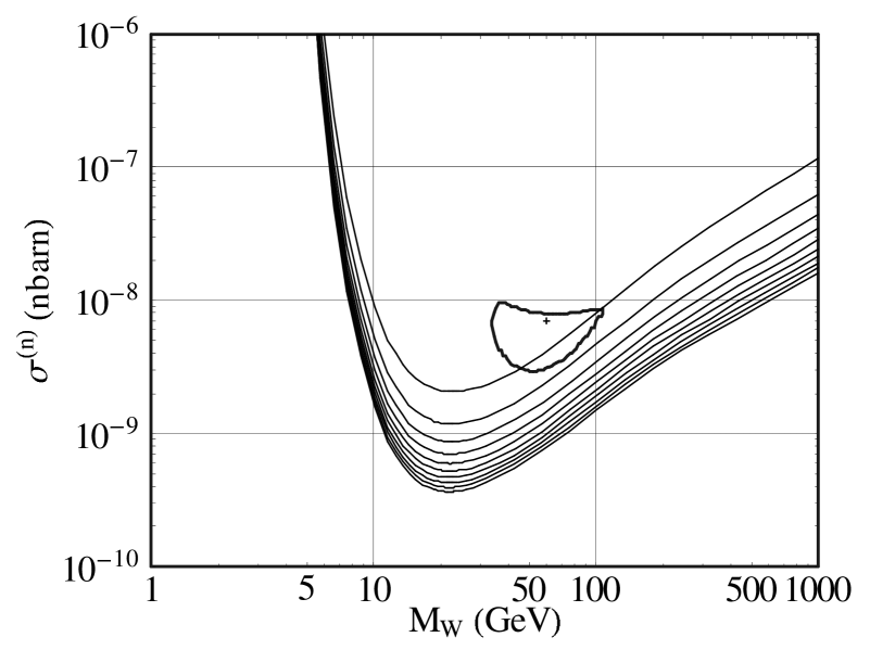
FIG. 1.: Sensitivity plots in the $\sigma^{(n)}$–$m_{W}$ plane for a germanium detector with threshold energy E_th=2 keV, flat background b=0.01 cpd/kg/keV and calculated for $<\delta^{2}>$=5.6. The set of curves correspond to different values of the exposure, MT$\alpha$=10 to 100 kg$\cdot$year in steps of 10 from top to bottom. The closed contour represents the 2$\sigma$ C.L. region singled out by the modulation analysis performed by the DAMA experiment[5] and the cross indicates the minimum of the likelihood found by the same authors.

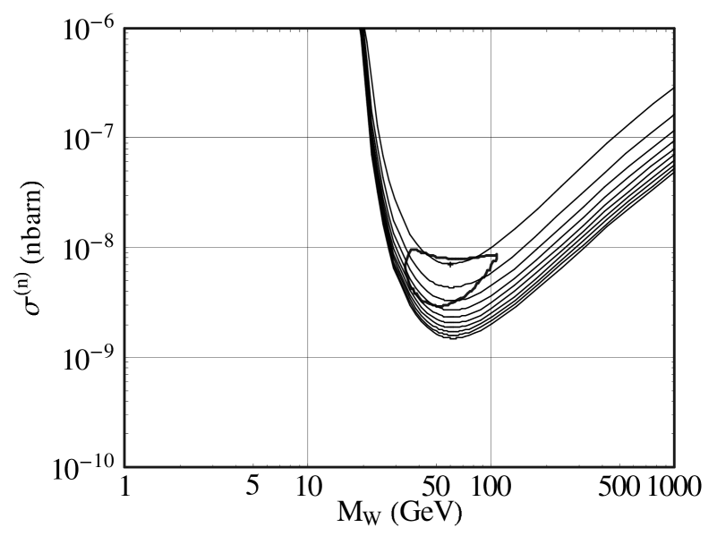
FIG. 2.: The same as in Figure 1 for a germanium detector with threshold energy E_th=12 keV.

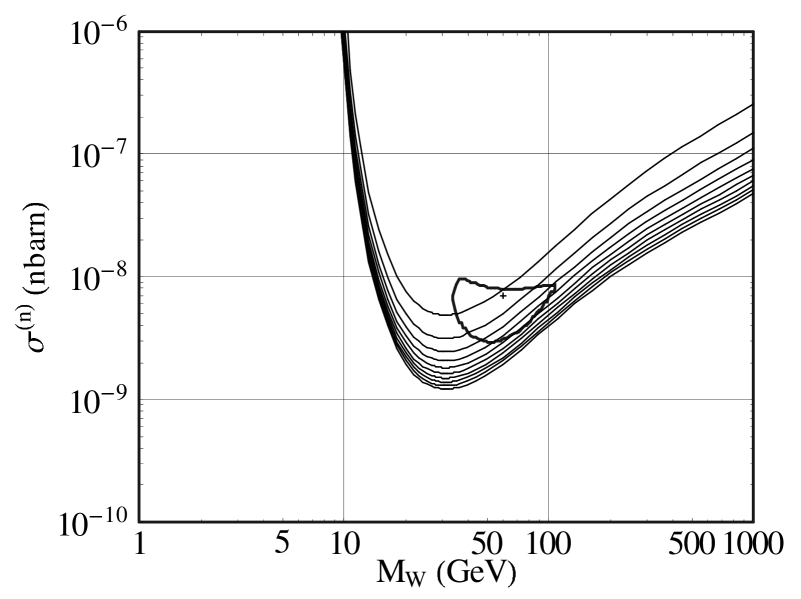
FIG. 3.: The same as in Figure 1 for a germanium detector with threshold energy E_th=4 keV and flat background b=0.1 cpd/kg/keV.

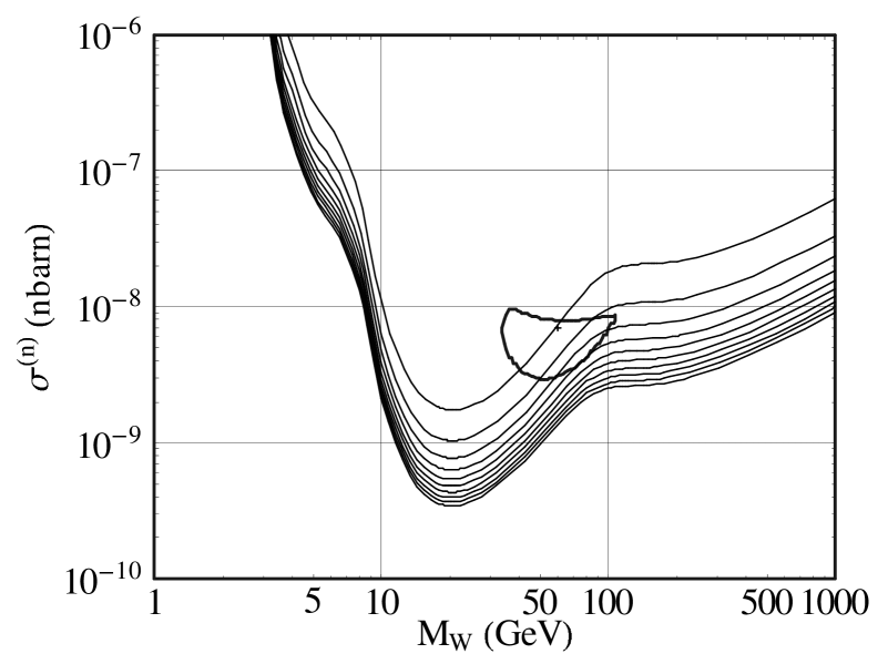
FIG. 4.: The same as in Figure 1 for a TeO₂ detector with threshold energy E_th=5 keV and flat background b=0.01 cpd/kg/keV.

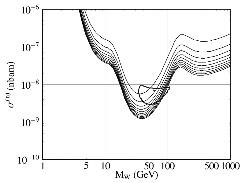
FIG. 5.: The same as in Figure 1 for an NaI detector with threshold energy E_th=2 keV and flat background b=0.1 cpd/kg/keV.

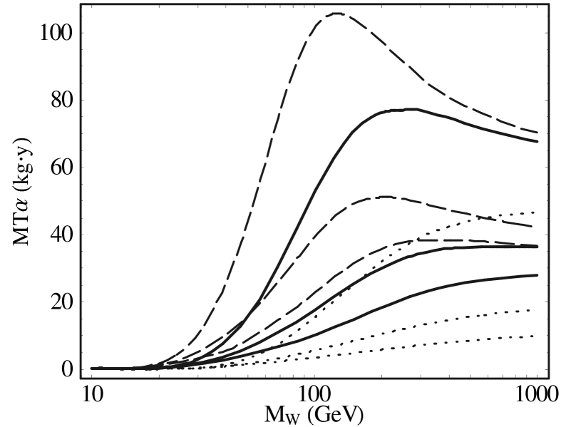
FIG. 6.: Minimal exposure MT$\alpha$ as a function of the WIMP mass $m_{W}$ required for the $<\delta^{2}>$=5.6 sensitivity plot to reach the exclusion plot of Ref.[5] to the WIMP–nucleon scalar cross section $\sigma^{(n)}$, and calculated for a germanium detector with threshold energy E_th=2 keV. Dotted, solid and dashed curves refer to $v_{\rm loc}$= 170, 220 and 270 km sec^-1 respectively. For each value of $v_{\rm loc}$ the curves calculated for a flat background b=0,0.01 and 0.1 cpd/kg/keV are given from bottom to top.

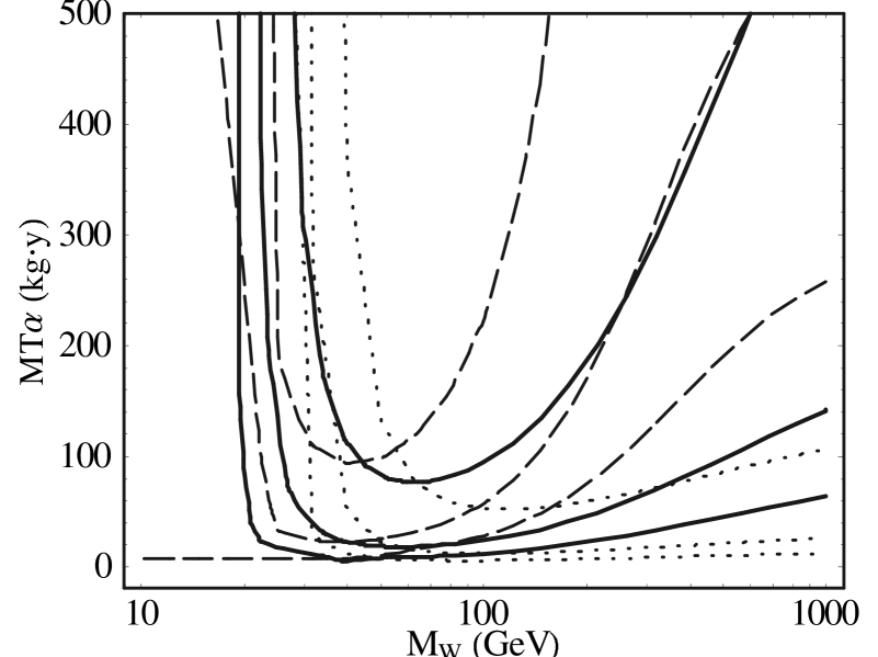
FIG. 7.: The same as in Figure 6 for a germanium detector with threshold energy E_th=12 keV.

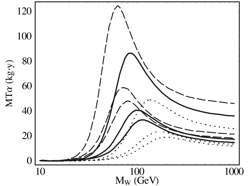
FIG. 8.: The same as in Figure 6 for a TeO₂ detector with threshold energy E_th=5 keV.

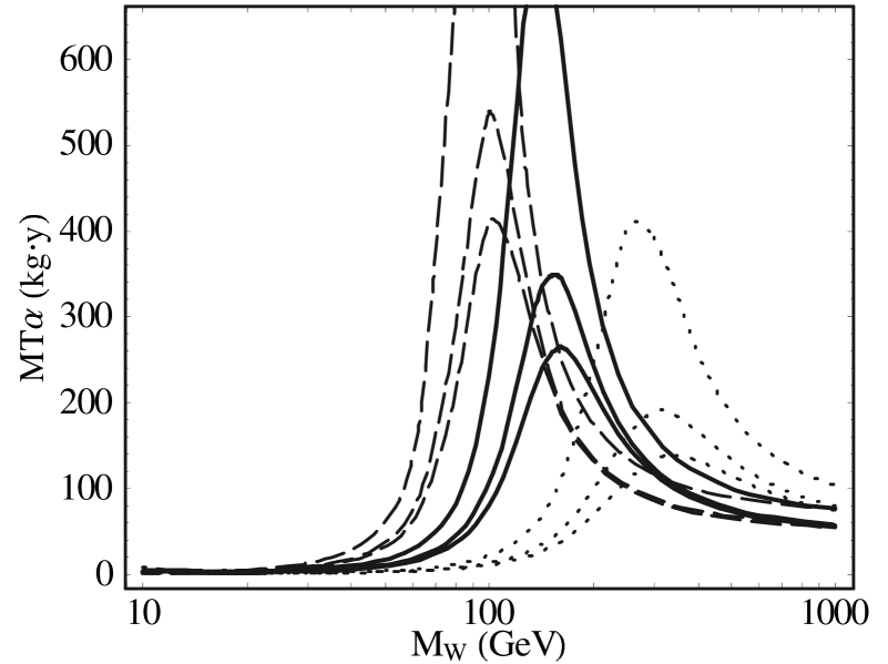
FIG. 9.: The same as in Figure 6 for an NaI detector with threshold energy E_th=2 keV.

REFERENCES

- [1] A. Drukier, K. Freese and D. Spergel, Phys. Rev. D33 (1986) 3495.
- [2] M.L. Sarsa, A. Morales, J. Morales, E. Garcia, A. Ortiz de Solorzano, J. Puimedon, C. Saenz, A. Salinas, J.A. Villar, Phys. Lett. B386 (1996) 458.
- [3] D. Abriola, F.T. Avignone, III, R.L. Brodzinski, J.I. Collar, D.E. Di Gregorio, H.A. Farach, E. Garcia, A.O. Gattone, C.K. Guerard, F. Hasenbalg, H. Huck, H.S. Miley, A. Morales, J. Morales, A. Ortiz de Solorzano, J. Puimedon, J.H. Reeves, A. Salinas, M.L. Sarsa, J.A. Villar, Astrop. Phys. 10 (1999) 133.
- [4] P. Belli, R. Bernabei, W. Di Nicolantonio, V. Landoni, F. Montecchia, A. Incicchitti, D. Prosperi, C. Bacci, O. Besida, C.J. Dai, Nuovo Cim. C19 (1996) 537.
- [5] R. Bernabei, P. Belli, F. Montecchia, W. Di Nicolantonio, A. Incicchitti, D. Prosperi, C. Bacci, C.J. Dai, L.K. Ding, H.H. Kuang and J.M. Ma, Phys. Lett. B424 (1998) 195; R. Bernabei, P. Belli, F. Montecchia, W. Di Nicolantonio, G. Ignesti, A. Incicchitti, D. Prosperi, C.J. Dai, L.K. Ding, H.H. Kuang and J.M. Ma, Phys. Lett. B450 (1999) 448.
- [6] K. Freese, J. Frieman and A. Gould, Phys. Rev. D37 (1988) 3388.
- [7] Y. Ramachers, M. Hirsch, H.V. Klapdor–Kleingrothaus, Eur. Phys. J. A3 (1998) 93.
- [8] F. Hasenbalg, Astrop. Phys. 9 (1998) 339.
- [9] See, for instance, G. Jungman, M. Kamionkowski and K. Griest, Phys. Rep. 267 (1996) 195, and references therein.
- [10] Review of particle properties, Particle Data Group, The European Physical Journal C3 (1998) 1.
- [11] L. Baudis, J. Hellmig, G. Heusser, H.V. Klapdor-Kleingrothaus, S. Kolb, B. Majorovits, H. Pas, Y. Ramachers, H. Strecker, V. Alexeev, A. Bakalyarov, A. Balysh, S.T. Belyaev, V.I. Lebedev, S. Zhukov, Phys. Rev. D59 (1999) 022001.
- [12] A. Morales, Direct Detection of WIMP Dark Matter, review talk given at the Sixth international workshop on Topics in Astroparticle and Underground Physics (TAUP99), Paris, 6–10 september 1999, to be published in Nucl. Phys. B(Proc. Suppl).
- [13] R. Gaitskell, Latest Results from the CDMS Collaboration, talk given at the Sixth international workshop on Topics in Astroparticle and Underground Physics (TAUP99), Paris, 6–10 september 1999, to be published in Nucl. Phys. B(Proc. Suppl).
- [14] M. Pavan, The first step toward CUORE: CUORICINO a 56 thermal detector array to search for rare events, talk given at the Sixth international workshop on Topics in Astroparticle and Underground Physics (TAUP99), Paris, 6–10 september 1999, to be published in Nucl. Phys. B(Proc. Suppl).
- [15] P.Belli, R. Bernabei, A. Bottino, F. Donato, N. Fornengo, D. Prosperi and S. Scopel, hep-ph/9903501; M. Brhlik and L. Roszkowski, Phys. Lett. B464 (1999) 303.
- [16] E. Garcia, A. Morales, J. Morales, M.L. Sarsa, A. Ortiz de Solorzano, E. Cerezo, R. Nunez-Lagos, J. Puimedon, C. Saenz, A. Salinas, J.A. Villar, J.I. Collar, F.T. Avignone, Phys. Rev. D51 (1995) 1458.
- [17] R. Bernabei, P. Belli, F. Montecchia, W. Di Nicolantonio, G. Ignesti, A. Incicchitti, D. Prosperi, C.J. Dai, L.K. Ding, H.H. Kuang and J.M. Ma, Phys. Lett. B450 (1999) 448.