Finite-volume analysis of
$N_{f}$-induced chiral phase transitions

Abstract

In the framework of Euclidean QCD on a torus, we study the spectrum of the Dirac operator through inverse moments of its eigenvalues, averaged over topological sets of gluonic configurations. The large-volume dependence of these sums is related to chiral order parameters. We sketch how these results may be applied to lattice simulations in order to investigate the chiral phase transitions occurring when $N_{f}$ increases. In particular, we demonstrate how Dirac inverse moments at different volumes could be compared to detect in a clean way the phase transition triggered by the suppression of the quark condensate and by the enhancement of the Zweig-rule violation in the vacuum channel.

Pacs numbers: 11.30.Rd, 12.39.Fe, 12.38.Gc, 02.70.Fj.

Contents

toc

I Introduction

Understanding the Spontaneous Breakdown of Chiral Symmetry (SB$\chi$S) remains one of the most challenging non-perturbative problems of QCD. Forthcoming experiments [1, 2, 3] should reveal some of its features, at least in the non-strange sector in which the effective number of light quark flavours is minimal ($N_{f}=2$). It is generally expected that if $N_{f}$ increases (keeping the number of colours $N_{c}$ fixed), the theory meets phase transitions and the chiral symmetry is eventually restored. The argument is originally based on properties of the QCD $\beta$-function in perturbation theory. The well-known statement of the “end of asymptotic freedom” for $N_{f}\geq 11N_{c}/2$ [4] has been further completed by the analysis of the so-called “conformal window” [5] suggesting a restoration of chiral symmetry for lower $N_{f}$, such as $N_{f}\sim 10$ (for $N_{c}=3$) [6]. Less perturbative and more model-dependent investigations, based on a gap equation [7] or on a “liquid instanton model” [8], also indicate that a chiral phase transition could occur for $N_{f}$ substantially below $11N_{c}/2$.

It is important to understand, at least qualitatively, the non-perturbative origin of the suppression of chiral order parameters for an increasing $N_{f}$. We have recently argued [9] that such a suppression might result from a paramagnetic effect of light (massless) quark loops [10], i.e. it could be due to “sea quarks” and, consequently, it could escape a detection in quenched lattice simulations, or in any other approach neglecting the fermion determinant. An appropriate framework to develop these ideas and to ask precise questions is the formulation of QCD in an Euclidean box $L\times L\times L\times L$, with periodic (antiperiodic) boundary conditions for gluon (fermion) fields, up to a gauge transformation. In this framework, the SB$\chi$S pattern is reflected by the dynamics of lowest eigenvalues of the Dirac operator:

$$H[G]=\gamma_{\mu}(\partial_{\mu}+iG_{\mu}).$$ (1)

This Hermitian operator has a symmetric spectrum with respect to zero: $\{H,\gamma_{5}\}=0$. Positive eigenvalues $\lambda_{n}$ are labeled in ascending order by a positive integer (one further denotes $\lambda_{-n}=-\lambda_{n}$ and $\phi_{-n}=\gamma_{5}\phi_{n}$ for the corresponding eigenvectors). SB$\chi$S is related to a particularly dense accumulation of eigenvalues around zero [11, 12, 13, 21]. Models of such an accumulation in terms of random matrices [14] or instantons [15] have been proposed. Some chiral order parameters are entirely dominated by the infrared extremity of the spectrum of the Dirac operator (1). This makes them particularly sensitive to the statistical weight given to smallest Dirac eigenvalues in the functional integral, which is suppressed in the massless limit by the $N_{f}$-th power of the fermion determinant. A good example is the quark condensate, defined by:

$$\Sigma(N_{f})=-\lim_{m_{1},m_{2},\ldots m_{N_{f}}\to 0}\langle 0|\bar{u}u|0\rangle,$$ (2)

where $m_{1}$…$m_{N_{f}}$ denote the $N_{f}$ lightest quark masses and $u$ represents the lightest quark field. $\Sigma(N_{f})$ receives exclusive contributions from the smallest Dirac eigenvalues that behave in average as $1/L^{4}$, and it is consequently expected to be the most sensitive order parameter to the variation of $N_{f}$ and to a phase transition. Other order parameters are less sensitive, like $F^{2}(N_{f})$, defined as the ${\rm SU}_{L}(N_{f})\times{\rm SU}_{R}(N_{f})$ limit of the coupling of the Goldstone bosons to the axial current:

$$F^{2}(N_{f})=\lim_{m_{1},m_{2},\ldots m_{N_{f}}\to 0}F^{2}_{\pi}.$$ (3)

$F^{2}(N_{f})$ may be non-zero due to Dirac eigenvalues accumulating as $1/L^{2}$ [13]. For this reason, $F^{2}(N_{f})$ should exhibit a weaker $N_{f}$-dependence than $\Sigma(N_{f})$. Finally, observables with no particular sensitivity to the infrared edge of the Dirac spectrum ($\rho$-mass, string tension, etc…) have no reason to be strongly affected by the fermion determinant and by the $N_{f}$-dependence.

Let us first consider the thermodynamical limit and denote by $n_{\rm crit}(N_{c})$ the critical value of $N_{f}$ at which the first chiral phase transition takes place. Just below $n_{\rm crit}(N_{c})$, the order parameter $\Sigma(N_{f})$ drops out, whereas its fluctuations may be expected to become important. We have shown [9] that the latter would manifest itself by an enhancement of the Zweig-rule violation just in the vacuum channel $J^{PC}=0^{++}$. An important Zweig-rule violation is precisely observed in the scalar channel [16], and nowhere else (with the exception of the pseudoscalar channel driven by the axial anomaly). Whilst the signature of a nearby phase transition is rather clear just below $n_{\rm crit}(N_{c})$, it is more speculative and ambiguous above the critical point. First, above $n_{\rm crit}(N_{c})$, colour might still be confined (confinement has no obvious relation to small Dirac eigenvalues). Second, despite $\Sigma(N_{f})=0$, the chiral symmetry need not be completely restored. The Goldstone bosons coupling to conserved axial currents with the strength $F(N_{f})$ might survive to the $N_{f}$-induced phase transition. This is reflected by the possibility that the $N_{f}$-sensitivity and suppression of the order parameter $F^{2}(N_{f})$ might be considerably weaker than in the case of the quark condensate [13]. Of course, this is a highly non-trivial possibility, which presumably depends on the existence of a non-perturbative fixed point in the renormalization group flow. Here, we take as a working hypothesis that above $n_{\rm crit}(N_{c})$, a partial SB$\chi$S still occurs, due to $F^{2}(N_{f})\neq 0$. The results of our paper allow, in particular, to test this hypothesis.

The central question remains how far is $n_{\rm crit}(N_{c})$ (for $N_{c}=3$) from the real world, in which the number of light quarks hardly exceeds $N_{f}=2-3$. Some recent investigations actually indicate that $n_{\rm crit}(3)$ could be rather small, and/or that the real world could already feel the influence of a nearby phase transition. First, some lattice simulations with dynamical fermions observe a strong $N_{f}$-dependence of SB$\chi$S signals for $N_{f}$ as low as 4-6 [18, 19]. Second, a method based on a well-convergent chiral sum rule has been proposed, which allows to study phenomenologically the variation of $\Sigma(N_{f})$ for small $N_{f}$ [20]. It has been found that existing experimental information on the Zweig-rule violation in the scalar channel leads to a large reduction of $\Sigma(N_{f})$ already between $N_{f}=2$ and $N_{f}=3$.

The purpose of this paper is to analyze in a model-independent way how $N_{f}$-induced chiral phase transitions manifest themselves in the finite-volume partition function. In particular, we shall investigate the volume dependence of the inverse spectral moments of the Dirac operator (1):

$$\sigma_{k}=\sum_{n>0}\frac{1}{(\lambda_{n}[G])^{k}},$$ (4)

averaged over topological sets of gluonic configurations. For $N_{f}\ll n_{\rm crit}(N_{c})$, the leading large-volume behaviour of such inverse moments has been worked out in details by Leutwyler and Smilga [21]. In order to investigate how this result is modified in the vicinity and above $n_{\rm crit}(N_{c})$, we rely on the basic observations and methods of Ref. [21]. For large sizes of the box ($\Lambda_{H}L\gg 1$ with $\Lambda_{H}\sim 1$ Gev), heavy excitations are exponentially suppressed in the partition function, which is then dominated by the lightest states, the pseudo-Goldstone bosons of SB$\chi$S. This leads to an effective description in terms of the Chiral Perturbation Theory ($\chi$PT) [22, 23], and it can be matched with QCD, yielding the desired information concerning the infrared properties of the Dirac spectrum. Moreover, the effective Lagrangian is identical to its infinite-volume counterpart, provided that periodic boundary conditions are used [24].

If $N_{f}$ lies far below $n_{\rm crit}(N_{c})$, the quark condensate is large and $\sigma_{k}$ behaves at large (but finite) volumes according to the asymptotic behaviour derived by Leutwyler and Smilga [21], using Standard $\chi$PT [22]. Above $n_{\rm crit}(N_{c})$, the quark condensate vanishes, and the previous analysis cannot be applied. However, if chiral symmetry is still partially broken, the matching with $\chi$PT remains possible and it leads to a clear-cut change in the large-volume behaviour of $\sigma_{k}$ : expressed through their inverse moments, the average behaviour of the lowest eigenvalues for $L\to\infty$ should turn from $1/L^{4}$ ($\langle\bar{q}q\rangle\neq 0$) into $1/L^{2}$ $(\langle\bar{q}q\rangle=0)$ [13]. When we approach the critical point with $N_{f}$ near but under $n_{\rm crit}(N_{c})$, significant discrepancies from the asymptotic limit $L\to\infty$ could be seen for large but finite boxes. The latter should then be analyzed using the framework of Generalized $\chi$PT [23, 35]. We have clearly in mind the possibility to use unquenched lattice simulations, varying $N_{f}$ and (finite) lattice size $L$ to eventually detect chiral phase transitions, through the volume dependence of inverse moments (4).

This article is organized as follows. In Sec. 2, we briefly review features of Euclidean QCD and of the effective theory on a torus. Sec. 3 explains how both theories are matched to derive the original form of Leutwyler-Smilga sum rules below $n_{\rm crit}(N_{c})$, before analyzing how they are modified in the phase where the quark condensate vanishes. In Sec. 4, we discuss the approach to the critical point, where a competition between a small quark condensate and higher order contributions leads to sizeable computable finite-volume effects. Sec. 5 is devoted to the computation of the next-to-leading-order corrections to the sum rules. We discuss in Sec. 6 how to obtain from the inverse moments an unambiguous signal indicating that $N_{f}$ approaches $n_{\rm crit}(N_{c})$, and we discuss the interest of lattice simulations in this framework. Sec. 7 summarizes the main results of this work.

II Small mass and large volume expansion of the partition function

A Euclidean QCD on a torus

The Euclidean QCD Lagrangian for $N_{f}$ light quarks reads:

$${{\cal L}}^{(N_{f})}=\frac{1}{4g^{2}}G^{a}_{\mu\nu}G^{a}_{\mu\nu}-i\theta\nu-i\bar{q}D\hbox to0.0pt{\hss/\,}q+\bar{q}\tilde{M}{q},$$ (5)

with the winding number density:

$$\nu(x)=\frac{1}{32\pi^{2}}G^{a}_{\mu\nu}(x)\tilde{G}^{a}_{\mu\nu}(x),$$ (6)

and the vacuum angle $\theta$ [25]. The quark mass matrix $\tilde{M}$ is of the form:

$$\tilde{M}=\frac{1}{2}(1-\gamma_{5})M+\frac{1}{2}(1+\gamma_{5})M^{\dagger},$$ (7)

where $M$ is a $N_{f}\times N_{f}$ complex matrix, diagonal in a suitable quark basis with positive real eigenvalues.

We consider the partition function of this Euclidean theory in a finite box $L\times L\times L\times L$, large enough to neglect safely the heavy quarks:

$$Z^{\theta}(N_{f})={{\cal C}}\int[dG]\int[d\bar{\psi}][d\psi]\exp\left(-\int_{V}d^{4}x\ {{\cal L}}^{(N_{f})}\right),$$ (8)

where ${\cal C}$ is a normalization constant, which may depend on the volume, but not on the mass matrix.

We impose boundary conditions on the fields, by viewing the box as a torus and identifying $x_{\mu}$ and $x_{\mu}+n_{\mu}L$ (with $n_{\mu}$ integers): the gluon fields have to be periodic and the quark fields antiperiodic in the four directions, up to a gauge transformation. The gauge fields are classified with respect to their winding number $\nu=\int_{V}dx\ \nu(x)$, which is a topologically invariant integer (related to the gauge transformation defining the periodicity of the fields on the torus). The index theorem asserts that $\nu$ is the difference between the number of left-handed and right-handed Dirac eigenvectors with a vanishing eigenvalue.

The Dirac eigenvalues satisfy a uniform bound [11]:

$$|\lambda_{n}[G]|<C\frac{n^{1/d}}{L}\equiv\omega_{n}.$$ (9)

This bound means essentially that an external gauge field lowers the eigenvalues of the free field theory [10]. It involves a coefficient $C$, depending only on the geometry of the space-time manifold, but neither on $G$, $n$ or $V=L^{d}$. The partition function $Z$ can be decomposed in Fourier modes over the winding number:

$$Z^{\theta}(N_{f})=\sum_{\nu=-\infty}^{\infty}e^{i\nu\theta}Z_{\nu}(N_{f}).$$ (10)

Each projection of positive winding number $\nu$ is:

$$Z_{\nu}(N_{f}) = {{\cal C}}\int_{\nu}[dG]e^{-S_{{\rm YM}}[G]}\det(-iD\hbox to0.0pt{\hss/\,}+\tilde{M})$$ (11)

$$= {{\cal C}}\int_{\nu}[dG]e^{-S_{{\rm YM}}[G]}({{\rm det}}_{f}M)^{\nu}{\prod_{n}}^{\prime}\left[\frac{{\det}_{f}(\lambda_{n}^{2}+MM^{\dagger})}{(\omega_{n}^{2}+\mu^{2})^{N_{f}}}\right],$$ (12)

$\int_{\nu}$ denotes the integration over the set of the gluonic configurations with a fixed winding number $\nu$, and $S_{{\rm YM}}$ is the pure gluonic action. $\det_{f}M$ is the determinant of the $N_{f}\times N_{f}$ quark mass matrix (it is replaced by $(\det_{f}M^{\dagger})^{-\nu}$ for $\nu\leq 0$). The primed product includes only the strictly positive eigenvalues: its denominator involves the Vafa-Witten bound $\omega_{n}$ of Eq. (9) and a reference mass scale $\mu$ larger than any light quark mass. It represents a convenient normalization of the determinant, such that each factor of the primed product is lower than 1 when the quark masses tend to zero. This normalization does not affect any observable. We check that the quark mass matrix and the vacuum angle arise in the partition function through the product $M\exp(i\theta/N_{f})$, consistently with the anomalous Ward identity for the singlet axial-vector current.

The partition function for a fixed positive winding number is:

$$Z_{\nu}(N_{f}) = {{\cal C}}\int_{\nu}[dG]e^{-S_{{\rm YM}}[G]}(\det_{f}M)^{\nu}$$ (14)

$$\qquad\times\left({\prod_{n}}^{\prime}\frac{\lambda_{n}^{2}}{\omega_{n}^{2}+\mu^{2}}\right)^{N_{f}}\exp\left[\left\langle{\sum_{n}}^{\prime}\log\left(1+\frac{MM^{\dagger}}{\lambda_{n}^{2}}\right)\right\rangle\right],$$

where $\langle\rangle$ denotes the trace over flavours. Provided that the partition function is regularized, we can expand the logarithm for small masses (compared to the size of the box):

$$Z_{\nu}(N_{f}) = {{\cal C}}\int_{\nu}[dG]e^{-S_{{\rm YM}}[G]}(\det_{f}M)^{\nu}\left({\prod_{n}}^{\prime}\frac{\lambda_{n}^{2}}{\omega_{n}^{2}+\mu^{2}}\right)^{N_{f}}$$ (16)

$$\qquad\times\exp\left[\langle M^{\dagger}M\rangle\sigma_{2}-\frac{1}{2}\langle(M^{\dagger}M)^{2}\rangle\sigma_{4}+O(M^{6})\right]$$

$$= {{\cal C}}^{\prime}_{\nu}(\det_{f}M)^{\nu}\left[1+\langle M^{\dagger}M\rangle\left\langle\!\left\langle\sigma_{2}\right\rangle\!\right\rangle_{\nu}^{(N_{f})}-\frac{1}{2}\langle(M^{\dagger}M)^{2}\rangle\left\langle\!\left\langle\sigma_{4}\right\rangle\!\right\rangle_{\nu}^{(N_{f})}\right.$$ (18)

$$\qquad\qquad\qquad\left.+\frac{1}{2}\langle M^{\dagger}M\rangle^{2}\left\langle\!\left\langle(\sigma_{2})^{2}\right\rangle\!\right\rangle_{\nu}^{(N_{f})}+O(M^{6})\right].$$

The inverse moments are defined for each gluonic configuration as: $\sigma_{k}={\sum_{n}}^{\prime}1/\lambda_{n}^{k}$. The normalization factor ${\cal C}^{\prime}_{\nu}$ is independent of the quark mass matrix:

$${{\cal C}}^{\prime}_{\nu}={{\cal C}}\int_{\nu}[dG]e^{-S_{{\rm YM}}[G]}\left({\prod}^{\prime}_{n}\frac{\lambda^{2}_{n}}{\omega_{n}^{2}+\mu^{2}}\right)^{N_{f}}.$$ (19)

The average over gluonic configurations with a given winding number is defined by

$$\left\langle\!\left\langle W\right\rangle\!\right\rangle_{\nu}^{(N_{f})}=\frac{\int_{\nu}[dG]e^{-S_{{\rm YM}}[G]}\left({\prod}^{\prime}_{n}\lambda^{2}_{n}\right)^{N_{f}}\ W}{\int_{\nu}[dG]e^{-S_{{\rm YM}}[G]}\left({\prod}^{\prime}_{n}\lambda^{2}_{n}\right)^{N_{f}}}.$$ (20)

where the denominator is a normalization factor, $\left\langle\!\left\langle 1\right\rangle\!\right\rangle_{\nu}=1$. In Eq. (18), this average is applied to inverse moments $\sigma_{k}$ that are particularly sensitive to the infrared tail of the Dirac spectrum. On the other hand, $\left\langle\!\left\langle\right\rangle\!\right\rangle_{\nu}^{(N_{f})}$ includes a product over eigenvalues, which should suppress the statistical weight of the lowest eigenvalues when the number $N_{f}$ of massless flavours increases. The averaged inverse moments in the exponential of Eq. (18) could therefore exhibit a strong dependence on $N_{f}$.

(16) contains several sources of divergences. Let us first consider the gluonic configuration as a fixed external field. In the fermion sector, sums over the Dirac spectrum may diverge because of its ultraviolet tail. For $\lambda\to\infty$, the number of eigenvalues in $[\lambda,\lambda+\Delta\lambda]$ is given by the free theory:

$$\Delta n=\frac{N_{C}}{4\pi^{2}}V|\lambda|^{3}\Delta\lambda.$$ (21)

The expected ultraviolet divergences of the inverse moments have therefore to be subtracted. We can write:

$$\sigma_{2}=\tilde{\sigma}_{2}+D_{2}^{(N_{f})},\qquad\sigma_{4}=\tilde{\sigma}_{4}+D_{4}^{(N_{f})},$$ (22)

where the divergent part is included in $D$, and $\tilde{\sigma}$ is finite. For instance, we can choose an ultraviolet cutoff $\Lambda$ and define the integer $K$ such that $\omega_{K}=\Lambda$. The regularized inverse moments then read:

$$\tilde{\sigma}_{k}=\sum_{n=1}^{K}\frac{1}{(\lambda_{n})^{k}},$$ (23)

and the divergent parts behave (at the leading order  of the volume) like:

$$D_{2}^{(N_{f})}\sim V\Lambda^{2},\qquad D_{4}^{(N_{f})}\sim V\ln\Lambda.$$ (24)

These short-distance contributions are the same for all winding-number sectors. If we perform this splitting in Eq. (16), we obtain the regularized partition function $\tilde{Z}_{\nu}$ involving the inverse moments $\tilde{\sigma}$, multiplied by an exponential factor with divergent counterterms which contribute only to the vacuum energy:

$$Z_{\nu}(N_{f})=\tilde{Z}_{\nu}(N_{f})\exp\left[D_{2}^{(N_{f})}\langle M^{\dagger}M\rangle-\frac{1}{2}D_{4}^{(N_{f})}\langle(M^{\dagger}M)^{2}\rangle\right].$$ (25)

Secondly, the product over the eigenvalues in the fermion determinant of Eq. (20) needs a regularization already for a fixed gluonic configuration. Nevertheless, for observables dominated by the lowest Dirac eigenvalues, we expect less sensitivity to the ultraviolet tail of the determinant. If we split the product over eigenvalues into ultraviolet and infrared parts [9, 32]:

$$\Delta=\Delta_{{\rm IR}}\Delta_{{\rm UV}},\qquad\Delta_{{\rm IR}}=\prod_{n=1}^{K}\left(\frac{\lambda^{2}_{n}}{\omega_{n}^{2}+\mu^{2}}\right)^{N_{f}},$$ (26)

we can expect the gluonic average of the inverse moments to depend essentially on $\Delta_{{\rm IR}}$, with a weak sensitivity on $\Lambda$.

Up to now, the gauge configuration was viewed as an external field, but the integration over the gluonic fields leads to a third series of divergences. Fortunately, their regularization is rather disconnected from the fermion sector [26] (for instance, the cut-off may be chosen independently of $\Lambda$). For the purpose of this paper, it is sufficient to stick to a multiplicative renormalization of the mass matrix and the Dirac eigenvalues,

$$M\to Z_{m}M,\qquad\lambda_{n}\to Z_{m}\lambda_{n},$$ (27)

inducing a multiplicative renormalization for $\left\langle\!\left\langle\sigma_{k}\right\rangle\!\right\rangle_{\nu}^{(N_{f})}$. We shall only consider homogeneous quantities, like ratios of inverse moments with the same degree of homogeneity in $\lambda$: the problem of the renormalization in the gluonic sector is therefore discarded in the rest of this article.

B Effective Lagrangian

For large volumes, the massive states are exponentially suppressed. The partition function is therefore dominated by the $N_{f}^{2}-1$ pseudo-Goldstone bosons resulting from the Spontaneous Breakdown of Chiral Symmetry and described at low energies by the Chiral Perturbation Theory ($\chi$PT). The effective Lagrangian for Goldstone bosons is written as a double expansion in powers of the momenta $p$ and of the quark masses $m$:

$${\cal L}_{\rm eff}=\sum_{k,l}{\cal L}_{(k,l)},$$ (28)

where ${\cal L}_{(k,l)}$ gathers all terms contributing like $p^{k}m^{l}$. In Euclidean QCD, it has been shown that, on a large torus, the low energy constants in ${\cal L}_{{\rm eff}}$ are not affected by finite-size effects [24].

If $U(x)\in{\rm SU}(N_{f})$ collects the Goldstone fields, the partition function is:

$$Z^{\theta}(N_{f})=\int[dU]\exp\left[-\int_{V}d^{4}x\ {\cal L}_{\rm eff}^{(N_{f})}(U,\partial U,Me^{i\theta/N_{f}})\right].$$ (29)

In this framework, the projection on a given winding number yields [21]:

$$Z_{\nu}(N_{f}) = \int\frac{d\theta}{2\pi}\ e^{-i\nu\theta}\int[dU]\exp\left[-\int_{V}d^{4}x\ {\cal L}_{\rm eff}^{(N_{f})}(U,Me^{i\theta/N_{f}})\right]$$ (30)

$$= \frac{1}{2\pi}\int[d\tilde{U}](\det\tilde{U})^{\nu}\exp\left[-\int_{V}d^{4}x\ {\cal L}_{\rm eff}^{(N_{f})}(\tilde{U},M)\right],$$ (31)

with $\tilde{U}(x)=U(x)\exp(-i\theta/N_{f})$. The path integral over ${\rm SU}(N_{f})$ for the partition function $Z^{\theta}$ ends up with an integral over ${\rm U}(N_{f})$ for $Z_{\nu}$. Because of the invariance properties of the measures $[dU]$ and $[d\tilde{U}]$, we have for any $V_{1},V_{2}\in{\rm U}(N_{f})$:

$$Z_{\nu}(N_{f}|V_{1}MV_{2})=(\det V_{1}V_{2})^{\nu}Z_{\nu}(N_{f}|M).$$ (32)

The low-energy constants in ${\cal L}_{\rm eff}$ are volume-independent and $N_{f}$-dependent order parameters. In particular, a partial restoration of chiral symmetry would make some of them vanish. Since the relative size of these order parameters vary with $N_{f}$, the organization of the double expansion (28) depends on the phase in which the theory is considered.

1. If the number of light flavours $N_{f}$ is fixed below $n_{\rm crit}(N_{c})$, the quark condensate $\Sigma(N_{f})$ is the order parameter that dominates the description of SB$\chi$S for sufficiently small quark masses (or sufficiently large volumes). The leading order  of the effective Lagrangian involves only a kinetic term and a term linear in the quark mass matrix:

$${\cal L}_{2}^{(N_{f})}=\frac{1}{4}F^{2}(N_{f})\langle\partial_{\mu}U^{\dagger}\partial_{\mu}U\rangle-\frac{1}{2}\Sigma(N_{f})\langle U^{\dagger}M+M^{\dagger}U\rangle.$$ (33)

$F$ is the decay constant of the Goldstone bosons and $\Sigma(N_{f})$ is the quark condensate, introduced in Sec. I in Eqs. (3) and (2). The expansion of the effective Lagrangian is organized in this case through the standard power counting [22]: $\partial\sim p$, $M\sim p^{2}$, so that the next-to-leading order  is $O(p^{4})$.

2. On the other hand, for $N_{f}>n_{\rm crit}(N_{c})$, the quark condensate vanishes and we cannot rely on the previous description anymore. In this case, the leading-order Lagrangian is the sum of the kinetic term, ${\cal L}_{(2,0)}$, and of a term quadratic in the quark masses, ${\cal L}_{(0,2)}$:

$${\cal L}_{(2,0)}^{(N_{f})} = \frac{F^{2}(N_{f})}{4}\langle\partial_{\mu}U^{\dagger}\partial_{\mu}U\rangle,$$ (34)

$${\cal L}_{(0,2)}^{(N_{f})} = -\frac{1}{4}\left[{\cal A}(N_{f})\langle(U^{\dagger}M)^{2}+(M^{\dagger}U)^{2}\rangle+{\cal Z}_{S}(N_{f})\langle U^{\dagger}M+M^{\dagger}U\rangle^{2}\right.$$ (36)

$$\qquad\qquad\left.+{\cal Z}_{P}(N_{f})\langle U^{\dagger}M-M^{\dagger}U\rangle^{2}+{\cal H}(N_{f})\langle M^{\dagger}M\rangle\right].$$

${\cal L}_{(0,2)}$ appears in the standard $O(p^{4})$ Lagrangian at the next-to-leading order, and the low-energy constants ${\cal Z}_{S}$, ${\cal Z}_{P}$, ${\cal A}$ and ${\cal H}$ correspond respectively to $L_{6}$, $L_{7}$, $L_{8}$ and $H_{2}$ of Ref. [22]. In this phase, the counting used to perform the expansion at higher orders is modified [23]: $\partial\sim M\sim p$.

In the generic case $N_{f}\geq 3$ (the case of two flavours is commented in App. B), ${\cal A}$, ${\cal Z}_{S}$ and ${\cal Z}_{P}$ are order parameters of SB$\chi$S. They are related to the low-energy behaviour of two-point correlators of the scalar and pseudoscalar densities $S_{a}(x)=\bar{\psi}(x)t_{a}\psi(x)$ and $P_{a}(x)=\bar{\psi}(x)t_{a}i\gamma_{5}\psi(x)$, where $\{t_{a}\}$ are flavour matrices. ${\cal A}$ stems from $\langle S_{a}S_{b}-P_{a}P_{b}\rangle$. ${\cal Z}_{S}$ is given by the correlator $\langle S_{0}S_{0}\delta_{ab}-S_{a}S_{b}\rangle$, and ${\cal Z}_{P}$ by $\langle P_{0}P_{0}\delta_{ab}-P_{a}P_{b}\rangle$: ${\cal Z}_{S}$ and ${\cal Z}_{P}$ violate the Zweig rule in the scalar and pseudoscalar channels respectively.

${\cal H}$ is a high-energy counterterm, which is not an order parameter and cannot be measured in low-energy processes. Other similar counterterms arise at higher orders: they involve only the quark mass matrix $M$, but not the Goldstone boson fields $U$. These counterterms are needed to subtract short-distance singularities in QCD correlation functions of quark currents. Their general structure is dictated by the chiral symmetry, and it is reproduced by the high-energy counterterms on the level of the effective Lagrangian.

3. For $N_{f}$ just below the critical point $n_{\rm crit}(N_{c})$, we expect a small (but non-vanishing) condensate and a large Zweig-rule violation in the scalar sector [9]. Linear and quadratic mass terms in the effective Lagrangian may be of comparable size. To take into account this possibility, we include both of them in the leading order  of the Lagrangian:

$$\tilde{{\cal L}}_{2}^{(N_{f})} = \frac{1}{4}\left[F^{2}(N_{f})\langle\partial_{\mu}U^{\dagger}\partial_{\mu}U\rangle-2\Sigma(N_{f})\langle U^{\dagger}M+M^{\dagger}U\rangle\right.$$ (39)

$$\quad-{\cal A}(N_{f})\langle(U^{\dagger}M)^{2}+(M^{\dagger}U)^{2}\rangle-{\cal Z}_{S}(N_{f})\langle U^{\dagger}M+M^{\dagger}U\rangle^{2}$$

$$\quad\left.-{\cal Z}_{P}(N_{f})\langle U^{\dagger}M-M^{\dagger}U\rangle^{2}-{\cal H}(N_{f})\langle M^{\dagger}M\rangle\right].$$

This Lagrangian can be actually viewed as the lowest order of another systematic expansion scheme, defined by the generalized chiral counting [23]: $\partial\sim M\sim B\sim O(p)$. In this case, the next-to-leading order  counts as $O(p^{3})$.

The standard and generalized counting rules are only two different ways of expanding the same effective Lagrangian:

$${\cal L}_{{\rm eff}}={\cal L}_{2}+{\cal L}_{4}+\ldots=\tilde{{\cal L}}_{2}+\tilde{{\cal L}}_{3}+\ldots$$ (40)

At a given order in $p$, Generalized $\chi$PT includes terms relegated by Standard $\chi$PT to higher orders. At the lowest order, Eq. (39) can be applied even if the quark condensate dominates. On the other hand, the Standard $\chi$PT becomes inaccurate in the vicinity of the critical point where $\Sigma\sim 0$, whereas Generalized $\chi$PT may be more appropriate to describe the transition.

III Leading large-volume behaviour of the inverse moments

A Matching QCD and the effective theory

If we analyze perturbatively the partition function (29), the only difference from the case of an infinite volume lies in the meson propagator, because of the periodic boundary conditions:

$$G(x)=\frac{1}{V}\sum_{p}\frac{e^{ipx}}{M_{\pi}^{2}+p^{2}},$$ (41)

where $p_{\mu}=2\pi n_{\mu}/L$, with $n_{\mu}$ integers. The contribution of the mode $p=0$ in this propagator blows up when pions become massless [27]. Graphs containing such zero modes will diverge in the chiral limit, whereas the non-zero modes are suppressed in the large-volume limit: the fluctuations of the zero modes are not Gaussian and cannot be treated perturbatively. To cope with them, we split the Goldstone boson fields in two unitary matrices: $U(x)=U_{0}U_{1}(x)$, where the constant factor $U_{0}$ describes the zero modes and $U_{1}(x)$ the remaining non-zero modes.

In a first approximation, the Gaussian fluctuations of $U_{1}$ can be neglected and the path integral in $Z$ reduces to a group integral over constant ${\rm SU}(N_{f})$ matrices:

$$Z(N_{f})={\cal D}\int_{{\rm SU}(N_{f})}[dU_{0}]\exp\left[-V{\cal L}^{(N_{f})}_{{\rm eff}}(U_{0},M\exp(i\theta/N_{f})\right].$$ (42)

where $[dU_{0}]$ is the Haar measure over the group, and ${\cal D}$ a normalization constant, independent of the mass. The projection on a topological sector (31) becomes:

$$Z_{\nu}(N_{f})=\frac{1}{2\pi}{\cal D}\int_{{\rm U}(N_{f})}[d\tilde{U}_{0}](\det\tilde{U}_{0})^{\nu}\exp\left[-V{\cal L}^{(N_{f})}_{{\rm eff}}(\tilde{U}_{0},M)\right].$$ (43)

To simplify the notations, we replace $\tilde{U}_{0}$ by $U$ in the calculations at the leading order  of $Z_{\nu}$. In addition, the $N_{f}$-dependence of the low-energy constants will not be explicitly denoted from now on, unless its presence is mandatory for understanding.

We want to expand $Z_{\nu}$ with respect to the size of the box and to the quark mass matrix. Actually, Eq. (42) tells us how to organize this from the expansion of ${\cal L}_{{\rm eff}}$. At the leading order, the partition function will depend on a simple scaling variable $X=ML^{\kappa}$. Below $n_{\rm crit}(N_{c})$, we have $\kappa=4$ (c.f. Eq. (33)), whereas the phase with a vanishing condensate yields $\kappa=2$ (c.f. Eq. (39)). For small $X$, the expansion of $Z_{\nu}$ reads:

$$Z_{\nu} = {\cal N}_{\nu}(\det X)^{\nu}[1+a_{\nu}\langle X^{\dagger}X\rangle$$ (45)

$$\qquad+b_{\nu}\langle X^{\dagger}X\rangle^{2}+c_{\nu}\langle(X^{\dagger}X)^{2}\rangle+O(X^{6})],$$

where the coefficients ${\cal N}_{\nu}$, $a_{\nu}$, $b_{\nu}$, $c_{\nu}$ do not depend on $M$. This expansion is valid for $\nu\geq 0$: for a negative $\nu$, $(\det X^{\dagger})^{|\nu|}$ arises instead of $(\det X)^{\nu}$. The calculations are very similar in both cases, and our future results can be translated for any winding number by writing $|\nu|$ instead of $\nu$.

The QCD partition function was expanded as a polynomial in the quark masses in Eq. (18), leading to:

$$Z_{\nu} = {\cal C}^{\prime}_{\nu}L^{-\kappa\nu N_{f}}({\rm det}_{f}X)^{\nu}$$ (48)

$$\qquad\left[1+\frac{1}{L^{2\kappa}}\langle X^{\dagger}X\rangle\left\langle\!\left\langle\sigma_{2}\right\rangle\!\right\rangle_{\nu}^{(N_{f})}-\frac{1}{2L^{4\kappa}}\langle(X^{\dagger}X)^{2}\rangle\left\langle\!\left\langle\sigma_{4}\right\rangle\!\right\rangle_{\nu}^{(N_{f})}\right.$$

$$\qquad\quad\left.+\frac{1}{2L^{4\kappa}}\langle X^{\dagger}X\rangle^{2}\left\langle\!\left\langle(\sigma_{2})^{2}\right\rangle\!\right\rangle_{\nu}^{(N_{f})}+O(X^{6})\right].$$

By identifying the same powers of $X$ in both expansions, we obtain relations between parameters of the effective Lagrangian and the leading large-volume behaviour of inverse moments.

When we compare Eqs. (45) and (48), we have to take into account the divergences of the inverse moments $\sigma_{k}$, as stressed in Eq. (25):

$$Z_{\nu}=\tilde{Z}_{\nu}\exp\left[D_{2}\langle M^{\dagger}M\rangle-\frac{1}{2}D_{4}\langle(M^{\dagger}M)^{2}\rangle\right]\sim Z_{\nu}^{{\rm\chi PT}}.$$ (49)

These counterterms, built from traces of the quark mass matrix, are also present in the $\chi$PT expression of the partition function. Therefore, the divergent behaviour of the inverse moments (e.g $D_{2}$ for $\sigma_{2}$) is tracked by counterterms in the $\chi$PT Lagrangian (in this case, ${\cal H}$). Divergence-free sum rules are found by considering linear combinations where the related $\chi$PT counterterms cancel.

B $N_{f}\ll n_{\rm crit}(N_{c})$: Leutwyler-Smilga sum rules

This case has already been treated with great details in Ref. [21]. We briefly review the main steps of the derivation of Leutwyler-Smilga sum rules for the reader’s convenience. Eq. (43) yields at the leading order:

$$Z_{\nu}(N_{f})=\frac{1}{2\pi}{\cal D}\int_{{\rm U}(N_{f})}[dU](\det\ U)^{\nu}\exp\left[\frac{\Sigma V}{2}\langle U^{\dagger}M+M^{\dagger}U\rangle\right].$$ (50)

$VM\Sigma$ is the only parameter of the group integral, and the scaling variable is $X=ML^{4}$ ($\kappa=4$). In the general case of an arbitrary matrix $M$, a formula for the integral (50) is discussed in Ref. [28]. For our present purpose, it is however sufficient to follow the original method described in Ref. [21] to expand Eq. (50) in powers of $M$. We obtain the expansion coefficients $a_{\nu}$, $b_{\nu}$, …through two derivative operators, applied on both expressions of $Z_{\nu}$: the group integral (50) and the $X$-expansion (45). The latter gives:

$$\sum_{a}\frac{\partial}{\partial X_{a}}\frac{\partial}{\partial X_{a}^{*}}Z_{\nu}={\cal N}_{\nu}(\det X)^{\nu}$$ (51)

$$\qquad\qquad\qquad\times\left\{\frac{N_{f}K}{2}a_{\nu}+\langle X^{\dagger}X\rangle\left[(N_{f}K+1)b_{\nu}+(N_{f}+K)c_{\nu}\right]+O(X^{4})\right\},$$ (52)

and

$$\sum_{abcd}\langle t_{a}t_{b}t_{c}t_{d}\rangle\frac{\partial}{\partial X_{a}}\frac{\partial}{\partial X_{b}^{*}}\frac{\partial}{\partial X_{c}}\frac{\partial}{\partial X_{d}^{*}}Z_{\nu}={\cal N}_{\nu}(\det X)^{\nu}$$ (53)

$$\qquad\qquad\qquad\times\frac{N_{f}K}{8}\left\{(N_{f}+K)b_{\nu}+(N_{f}K+1)c_{\nu}+O(X^{2})\right\},$$ (54)

where $K=N_{f}+\nu$, and $X_{a}$ are the coordinates of $X$ on $\{t_{a}\}$ ($a=0\ldots N_{f}^{2}-1$), which is a complete set of Hermitian matrices (see App. A).

The same derivative operators are applied on the group integral (50):

$$\sum_{a}\frac{\partial}{\partial X_{a}}\frac{\partial}{\partial X_{a}^{*}}Z_{\nu} = \frac{1}{8}N_{f}\Sigma^{2}Z_{\nu},$$ (55)

$$\sum_{abcd}\langle t_{a}t_{b}t_{c}t_{d}\rangle\frac{\partial}{\partial X_{a}}\frac{\partial}{\partial X_{b}^{*}}\frac{\partial}{\partial X_{c}}\frac{\partial}{\partial X_{d}^{*}}Z_{\nu} = \frac{1}{256}N_{f}\Sigma^{4}Z_{\nu}.$$ (56)

Once $Z_{\nu}$ is replaced by its $X$-expansion (45) on the right hand-side of Eqs. (55) and (56), these equations yield polynomials in $X$, which are identified with Eqs. (51) and (53) order by order in powers of $X$. We get thus $a_{\nu}$, and a linear system of two equations for $b_{\nu}$ and $c_{\nu}$.

Once $a_{\nu}$, $b_{\nu}$ and $c_{\nu}$ computed, the comparison of Eqs. (45) and (48) leads to the Leutwyler-Smilga sum rules:

$$\left\langle\!\left\langle\sigma_{2}\right\rangle\!\right\rangle_{\nu}^{(N_{f})} = a_{\nu}=\frac{[V\Sigma(N_{f})]^{2}}{4K},$$ (57)

$$\left\langle\!\left\langle(\sigma_{2})^{2}\right\rangle\!\right\rangle_{\nu}^{(N_{f})} = 2b_{\nu}=\frac{[V\Sigma(N_{f})]^{4}}{16(K^{2}-1)},$$ (58)

$$\left\langle\!\left\langle\sigma_{4}\right\rangle\!\right\rangle_{\nu}^{(N_{f})} = -2c\nu=\frac{[V\Sigma(N_{f})]^{4}}{16K(K^{2}-1)}.$$ (59)

Because of $K=N_{f}+|\nu|$, the sum rules (57)-(59) depend explicitly on the number of flavours, but there is another (implicit and unknown) dependence stemming from the quark condensate $\Sigma(N_{f})$. No divergent counterterm is explicitly present: these sum rules are derived from the leading order  Lagrangian in Standard $\chi$PT, and they show only an asymptotic behaviour, valid for $V\to\infty$. For instance, $\sigma_{2}$ and $(\sigma_{2})^{2}$ contain divergent subleading terms.

C $N_{f}>n_{\rm crit}(N_{c})$: the phase with a vanishing quark condensate

For $N_{f}>n_{\rm crit}(N_{c})$, the integral defining $Z_{\nu}$ in terms of the effective Lagrangian (43) involves quadratic mass terms at the leading order:

$$Z_{\nu}(N_{f}) = \frac{1}{2\pi}{\cal D}\int_{{\rm U}(N_{f})}[dU](\det U)^{\nu}$$ (62)

$$\quad\times\exp\Bigg{[}\frac{V}{4}\left\{{\cal A}\langle(U^{\dagger}M)^{2}+(M^{\dagger}U)^{2}\rangle+{\cal Z}_{S}\langle U^{\dagger}M+M^{\dagger}U\rangle^{2}\right.$$

$$\qquad\qquad\qquad\left.+{\cal Z}_{P}\langle U^{\dagger}M-M^{\dagger}U\rangle^{2}+{\cal H}\langle M^{\dagger}M\rangle\right\}\Bigg{]}.$$

The scaling variable is now $X=ML^{2}$ ($\kappa=2$). The counterterm ${\cal H}$ has the same structure as the divergent term $D_{2}$ due to $\sigma_{2}$ in Eq. (49). To eliminate this divergence, it is natural to introduce the $\nu$-dependent fluctuation $\bar{\sigma}_{2}=\sigma_{2}-\left\langle\!\left\langle\sigma_{2}\right\rangle\!\right\rangle_{\nu}^{(N_{f})}$. The subtraction of this quadratic divergence leads to the loss of a single sum rule, for instance $\left\langle\!\left\langle\sigma_{2}\right\rangle\!\right\rangle^{(N_{f})}_{0}$. For the other topological sectors, we can indeed write sum rules concerning $\left\langle\!\left\langle\sigma_{2}\right\rangle\!\right\rangle_{\nu}^{(N_{f})}-\left\langle\!\left\langle\sigma_{2}\right\rangle\!\right\rangle_{0}^{(N_{f})}$, since the (short-distance) divergence due to ${\cal H}$ is insensitive to the (topological) winding number.

Because of chirality, the integral (62) vanishes unless the same power of $U$ and $U^{\dagger}$ arises. The determinant $(\det U)^{\nu}$ counts as the $\nu N_{f}$-th power of $U$, whereas the exponential involves only the square of $U^{\dagger}$. Therefore, the phase of an odd $N_{f}>n_{\rm crit}(N_{c})$ discriminates between the topological sectors: the odd-$\nu$ sectors are suppressed in the large-volume limit compared to the even winding numbers (this discrimination does not occur for an even number of flavours). As a matter of fact, the symmetry $M\to-M$ is equivalent to $\theta\to\theta+\pi N_{f}$. From the Fourier decomposition (10), we can directly check that the odd topological sectors have a vanishing partition function at the leading order, provided that $N_{f}$ is odd. Of course, higher orders of the effective Lagrangian (for instance $\tilde{{\cal L}}_{3}$) contribute to the odd topological sectors, giving finally rise for $Z_{\nu}$ to a different volume dependence from the even winding numbers.

In the topologically trivial sector $\nu=0$, $(\det U)^{\nu}$ disappears from the group integral and the exponential in (62) can be directly expanded in powers of $X$ and integrated over ${\rm U}(N)$. Using App. A, the computation of the lowest powers in the $X$-expansion is straightforward, leading to the sum rules:

$$\langle\!\langle\left(\bar{\sigma}_{2}\right)^{2}\rangle\!\rangle_{0} = \frac{V^{2}}{16N_{f}^{2}(N_{f}^{2}-1)}$$ (64)

$$\quad\times[4(2N_{f}^{2}+1)({\cal Z}_{S}^{2}+{\cal Z}_{P}^{2})-8{\cal Z}_{S}{\cal Z}_{P}-8N_{f}{\cal A}({\cal Z}_{S}+{\cal Z}_{P})+4N_{f}^{2}{\cal A}^{2}],$$

$$\langle\!\langle\sigma_{4}\rangle\!\rangle_{0} = \frac{V^{2}}{16N_{f}(N_{f}^{2}-1)}$$ (66)

$$\quad\times[12({\cal Z}_{S}^{2}+{\cal Z}_{P}^{2})-8{\cal Z}_{S}{\cal Z}_{P}-8N_{f}{\cal A}({\cal Z}_{S}+{\cal Z}_{P})+4{\cal A}^{2}].$$

As emphasized in the previous section, these sum rules depend on the number of massless flavours in an explicit way, but also implicitly through the $N_{f}$-dependent order parameters ${\cal A}$, ${\cal Z}_{S}$ and ${\cal Z}_{P}$.

These sum rules predict a different large-volume behaviour from the Leutwyler-Smilga sum rules (57)-(59). This agrees with our general expectation concerning the large-volume dependence of the (suitably averaged) small Dirac eigenvalues [13]. The eigenvalues accumulating like $1/L^{4}$ contribute to SB$\chi$S and to the quark condensate. Correspondingly, for $N_{f}<n_{\rm crit}(N_{c})$, the asymptotic behaviour of the sum rules is:

$$\left\langle\!\!\left\langle{\sum_{n}}^{\prime}\frac{1}{\lambda_{n}^{2}}\right\rangle\!\!\right\rangle_{0}\sim V^{2},\qquad\left\langle\!\!\left\langle{\sum_{n}}^{\prime}\frac{1}{\lambda_{n}^{4}}\right\rangle\!\!\right\rangle_{0}\sim V^{4}.$$ (67)

On the other hand, the $1/L^{2}$-eigenvalues do not contribute to the quark condensate, but may still contribute to SB$\chi$S in the phase above $n_{\rm crit}(N_{c})$, through a non-vanishing value of $F^{2}(N_{f})$. Indeed, Eqs. (64) and (66) predict in this phase an infinite-volume limit of $V^{2}$ for $\langle\!\langle\left(\bar{\sigma}_{2}\right)^{2}\rangle\!\rangle_{0}$ and $\langle\!\langle\sigma_{4}\rangle\!\rangle_{0}$, as expected.

IV The approach to the critical point

A Leading large-volume behaviour

We want now to study the intermediate case, where the linear and the quadratic mass terms in the effective Lagrangian may compete for some range of volumes. To understand which results can be expected, it is instructive to consider first $\chi$PT in an infinite volume and to imagine that we let the quark masses vary. If the quark condensate is (even slightly) different from zero, we can always find sufficiently small quark masses for which the linear mass term is dominant. When the quarks become massive, the corrections due to the quadratic mass terms may become discernible and even preponderant, provided that the quark condensate is not too large to hide their effects.

In this paper, we work in a box with a fixed large volume, and $M_{\pi}^{2}$ is counted as $O(1/L^{4})$. The variation of the quark masses is therefore translated into a change of the volume. For $N_{f}<n_{\rm crit}(N_{c})$, the Leutwyler-Smilga sum rules derived in S$\chi$PT should correctly describe the volume-dependence of the inverse moments when $L$ tends to infinity. However, close to the critical point and for a given value of the volume, the quark condensate need not be large enough to make ${\cal L}_{2}$, Eq. (33), dominate. This could lead to significant deviations from the asymptotic limit even for large volumes.

Hence, the leading order  of the Lagrangian is $\tilde{{\cal L}}_{2}$, Eq. (39), and $Z_{\nu}$ reads:

$$Z_{\nu} = \frac{1}{2\pi}{\cal D}\int_{{\rm U}(N_{f})}[dU](\det U)^{\nu}$$ (70)

$$\quad\times\exp\Bigg{[}\frac{V}{4}\left\{2\Sigma\langle U^{\dagger}M+M^{\dagger}U\rangle+{\cal A}\langle(U^{\dagger}M)^{2}+(M^{\dagger}U)^{2}\rangle\right.$$

$$\qquad\qquad\qquad\left.+{\cal Z}_{S}\langle U^{\dagger}M+M^{\dagger}U\rangle^{2}+{\cal Z}_{P}\langle U^{\dagger}M-M^{\dagger}U\rangle^{2}+{\cal H}\langle M^{\dagger}M\rangle\right\}\Bigg{]}.$$

$X=ML^{2}$ remains the scaling parameter for the mass, and $\Sigma L^{2}$ is the expansion variable for the quark condensate. This organizes the expansion through the power counting $\Sigma\sim M\sim 1/L^{2}$, similar to G$\chi$PT. We shall therefore consider the theory for volumes and masses so that $X$ and $\Sigma L^{2}$ are of order 1.

In order to evaluate (70), it is convenient to define the group integral $I_{\nu}$ for arbitrary complex numbers $(b,\bar{b},z,\bar{z},y,a,\bar{a})$:

$$I_{\nu} = \int_{{\rm U}(N_{f})}\ [dU]\ (\det U)^{\nu}$$ (73)

$$\qquad\times\exp[b\langle XU^{\dagger}\rangle+\bar{b}\langle X^{\dagger}U\rangle+z\langle XU^{\dagger}\rangle^{2}+\bar{z}\langle X^{\dagger}U\rangle^{2}$$

$$\qquad\qquad\qquad+y\langle XU^{\dagger}\rangle\langle X^{\dagger}U\rangle+a\langle(XU^{\dagger})^{2}\rangle+\bar{a}\langle(X^{\dagger}U)^{2}\rangle],$$

The partition function at a fixed winding number reads:

$$Z_{\nu}=\frac{1}{2\pi}{\cal D}\exp[h^{0}\langle X^{\dagger}X\rangle]I_{\nu}(b^{0},\bar{b}^{0},z^{0},\bar{z}^{0},y^{0},a^{0},\bar{a}^{0};X),$$ (74)

where $I_{\nu}$ is calculated with the values:

$$b^{0}=\bar{b}^{0}=\frac{1}{2}L^{2}\Sigma,$$ (75)

$$z^{0}\ =\ \bar{z}^{0}\ =\ \frac{1}{4}({\cal Z}_{S}+{\cal Z}_{P}), y^{0}\ =\ \frac{1}{2}({\cal Z}_{S}-{\cal Z}_{P}),$$ (76)

$$a^{0}\ =\ \bar{a}^{0}\ =\ \frac{1}{4}{\cal A}, h^{0}\ =\ \frac{1}{4}{\cal H}.$$ (77)

$I_{\nu}$ is a polynomial in $(b,\bar{b},z,\bar{z},y,a,\bar{a})$, and its derivatives are not independent:

$$\frac{\partial^{2}I_{\nu}}{\partial b^{2}}=\frac{\partial I_{\nu}}{\partial z}\qquad\frac{\partial^{2}I_{\nu}}{\partial\bar{b}^{2}}=\frac{\partial I_{\nu}}{\partial\bar{z}}\qquad\frac{\partial^{2}I_{\nu}}{\partial b\partial\bar{b}}=\frac{\partial I_{\nu}}{\partial y}$$ (78)

We expand this integral in powers of $X$, with coefficients that are independent of the quark mass matrix:

$$I_{\nu} = (\det X)^{\nu}[\alpha_{\nu}+\beta_{\nu}\langle X^{\dagger}X\rangle+\gamma_{\nu}\langle X^{\dagger}X\rangle^{2}+\delta_{\nu}\langle(X^{\dagger}X)^{2}\rangle$$ (80)

$$\qquad\qquad+\epsilon_{\nu}\langle X^{\dagger}X\rangle^{3}+\eta_{\nu}\langle(X^{\dagger}X)^{2}\rangle\langle X^{\dagger}X\rangle+\kappa_{\nu}\langle(X^{\dagger}X)^{3}\rangle+O(X^{8})],$$

We identify the same powers of $X$ in the expression of $Z_{\nu}$ in terms of averaged inverse moments (48) and in its expression at the leading order of the effective Lagrangian, obtained from Eqs. (74) and (80). This leads to the sum rules:

$$\langle\!\langle\sigma_{2}\rangle\!\rangle_{\nu}^{(N_{f})} = V\left(\frac{\beta_{\nu}}{\alpha_{\nu}}+h\right)$$ (81)

$$\langle\!\langle\left(\sigma_{2}\right)^{2}\rangle\!\rangle_{\nu}^{(N_{f})} = 2V^{2}\left(\frac{\gamma_{\nu}}{\alpha_{\nu}}+h\frac{\beta_{\nu}}{\alpha_{\nu}}+\frac{h^{2}}{2}\right)$$ (82)

$$\langle\!\langle\sigma_{4}\rangle\!\rangle_{\nu}^{(N_{f})} = -2V^{2}\frac{\delta_{\nu}}{\alpha_{\nu}}$$ (83)

$$\langle\!\langle\left(\bar{\sigma}_{2}\right)^{2}\rangle\!\rangle_{\nu}^{(N_{f})} = V^{2}\left(2\frac{\gamma_{\nu}}{\alpha_{\nu}}-\left(\frac{\beta_{\nu}}{\alpha_{\nu}}\right)^{2}\right)$$ (84)

$$\langle\!\langle\left(\bar{\sigma}_{2}\right)^{3}\rangle\!\rangle_{\nu}^{(N_{f})} = V^{3}\left(6\frac{\epsilon_{\nu}}{\alpha_{\nu}}-6\frac{\beta_{\nu}}{\alpha_{\nu}}\frac{\gamma_{\nu}}{\alpha_{\nu}}+2\left(\frac{\beta_{\nu}}{\alpha_{\nu}}\right)^{3}\right)$$ (85)

$$\langle\!\langle\bar{\sigma}_{2}\sigma_{4}\rangle\!\rangle_{\nu}^{(N_{f})} = V^{3}\left(-2\frac{\eta_{\nu}}{\alpha_{\nu}}+2\frac{\beta_{\nu}}{\alpha_{\nu}}\frac{\delta_{\nu}}{\alpha_{\nu}}\right)$$ (86)

$$\langle\!\langle\sigma_{6}\rangle\!\rangle_{\nu}^{(N_{f})} = 3V^{3}\kappa_{\nu}$$ (87)

If we know $\alpha_{\nu}$, $\beta_{\nu}$,…in terms of the low-energy constants of $\tilde{{\cal L}}_{2}$, Eqs. (81)-(87) lead to the desired sum rules. The high-energy counterterm $h$, which reflects the ultraviolet divergence in $\sigma_{2}$, has to be eliminated. This can be obtained if we consider the fluctuation of $\sigma_{2}$ over a topological sector: $\bar{\sigma}_{2}=\sigma_{2}-\left\langle\!\left\langle\sigma_{2}\right\rangle\!\right\rangle_{\nu}^{(N_{f})}$, as defined in Sec. III C.

For the topologically trivial sector $\nu=0$, the computation is very simple, following the same line as for the phase $N_{f}>n_{\rm crit}(N_{c})$. This leads to the expansion coefficients (for $b=\bar{b}$, $z=\bar{z}$, $a=\bar{a}$):

$$\alpha_{0} = 1\qquad\beta_{0}\ =\ \frac{1}{N_{f}}(y+b^{2})$$ (88)

$$\gamma_{0} = \frac{1}{N_{f}(N_{f}^{2}-1)}$$ (90)

$$\times\left\{N_{f}[\frac{b^{4}}{2}+2b^{2}y+2b^{2}z+y^{2}+2z^{2}+2a^{2}]-2a[b^{2}+2z]\right\}$$

$$\delta_{0} = \frac{1}{N_{f}(N_{f}^{2}-1)}$$ (92)

$$\times\left\{-[\frac{b^{4}}{2}+2b^{2}z+2b^{2}y+y^{2}+2z^{2}+2a^{2}]+N_{f}\cdot 2a[b^{2}+2z]\right\}$$

$$\epsilon_{0} = \frac{1}{N_{f}(N_{f}^{2}-1)(N_{f}^{2}-4)}$$ (95)

$$\times\left\{6(N_{f}^{2}-2)\left[\frac{b^{6}}{36}+b^{4}\left(\frac{z}{3}+\frac{y}{4}\right)+b^{2}\left(z^{2}+\frac{y^{2}}{2}+yz\right)+\left(\frac{y^{3}}{6}+yz^{2}\right)\right]\right.$$

$$\qquad\left.+2(N_{f}^{2}+2)\left[b^{2}+y\right]a^{2}-12N_{f}\left[\frac{b^{4}}{6}+b^{2}\left(\frac{y}{2}+z\right)+yz\right]a\right\}$$

$$\eta_{0} = \frac{1}{N_{f}(N_{f}^{2}-1)(N_{f}^{2}-4)}$$ (98)

$$\times\left\{-18N_{f}\left[\frac{b^{6}}{36}+b^{4}\left(\frac{z}{3}+\frac{y}{4}\right)+b^{2}\left(z^{2}+\frac{y^{2}}{2}+yz\right)+\left(\frac{y^{3}}{6}+yz^{2}\right)\right]\right.$$

$$\qquad\left.-18N_{f}\left[b^{2}+y\right]a^{2}+12(N_{f}^{2}+2)\left[\frac{b^{4}}{6}+b^{2}\left(\frac{y}{2}+z\right)+yz\right]a\right\}$$

$$\kappa_{0} = \frac{1}{N_{f}(N_{f}^{2}-1)(N_{f}^{2}-4)}$$ (101)

$$\left\{24\left[\frac{b^{6}}{36}+b^{4}\left(\frac{z}{3}+\frac{y}{4}\right)+b^{2}\left(z^{2}+\frac{y^{2}}{2}+yz\right)+\left(\frac{y^{3}}{6}+yz^{2}\right)\right]\right.$$

$$\qquad\left.+4(N_{f}^{2}+2)\left[b^{2}+y\right]a^{2}-24N_{f}\left[\frac{b^{4}}{6}+b^{2}\left(\frac{y}{2}+z\right)+yz\right]a\right\}$$

Before focusing on the resulting sum rules for the topologically trivial sector $\nu=0$, we sketch the general derivation of the expansion coefficients for an arbitrary winding number.

B Topologically non-trivial sectors: $\nu\neq 0$

Let us begin with the leading coefficient $\alpha_{\nu}$. Independent of $X$, it can be computed for $X=x\cdot 1$, where $x$ is a complex number. $\alpha_{\nu}$ is then given by the leading order  of $I_{\nu}$ in $x$ (without any power of $x^{*}$), and it depends only on $(b,z,a)$. As a matter of fact, $\alpha_{\nu}(b,z,a)$ can be deduced from $\alpha_{\nu}(b,0,a)$ because of the relations between the derivatives (78). The problem reduces to obtaining the leading order  in $x$ of the group integral:

$$I^{\alpha}_{\nu}=I_{\nu}(b,a;x\cdot 1)=\int_{{\rm U}(N_{f})}\ [dU](\det U)^{\nu}\exp[bx\langle U^{\dagger}\rangle+ax^{2}\langle{U^{\dagger}}^{2}\rangle].$$ (103)

The Appendix C 1 describes how $\alpha_{\nu}(b,0,a)$ is extracted from this integral, leading to the polynomial:

$$\alpha_{\nu}(b,z=0,a)=\sum_{m=0\ldots\nu N_{f}/2}b^{\nu N_{f}-2m}a^{m}c_{m},$$ (104)

where $\{c_{m}\}$ are purely combinatorial coefficients. Using $\partial^{2}\alpha_{\nu}/\partial b^{2}=\partial\alpha_{\nu}/\partial z$, we obtain the general expression of $\alpha_{\nu}$:

$$\alpha_{\nu}(b,z,a)=\sum_{l+2m+2p=\nu N_{f}}b^{l}a^{m}z^{p}\frac{(l+2p)!}{l!p!}c_{m}.$$ (105)

In the limit case of a vanishing quark condensate ($b=0$), we check that $\alpha_{\nu}$ (and therefore $I_{\nu}$) vanishes if $\nu N_{f}$ is odd, in agreement with the parity discrimination discussed in Sec. III C.

We obtain the next coefficients by applying the derivative operators of Eqs. (51) and (53) on both representations of $I_{\nu}$: the group integral (73) and the $X$-expansion (80). We already know the result of the latter from the phase $N_{f}\ll n_{\rm crit}(N_{c})$, studied in Sec III B:

$$\sum_{a}\frac{\partial}{\partial X_{a}}\frac{\partial}{\partial X_{a}^{*}}I_{\nu}$$ (106)

$$\qquad=(\det X)^{\nu}\left\{\frac{N_{f}K}{2}\beta_{\nu}+\langle X^{\dagger}X\rangle\left[(N_{f}K+1)\gamma_{\nu}+(N_{f}+K)\delta_{\nu}\right]+O(X^{4})\right\},$$ (107)

$$\sum_{abcd}\langle t_{a}t_{b}t_{c}t_{d}\rangle\frac{\partial}{\partial X_{a}}\frac{\partial}{\partial X_{b}^{*}}\frac{\partial}{\partial X_{c}}\frac{\partial}{\partial X_{d}^{*}}I_{\nu}$$ (108)

$$\qquad\qquad=(\det X)^{\nu}\frac{N_{f}K}{8}\left\{(N_{f}+K)\gamma_{\nu}+(N_{f}K+1)\delta_{\nu}+O(X^{2})\right\}.$$ (109)

The two-derivative operator, applied on the group integral (73) that defines $I_{\nu}$, leads to:

$$\sum_{a}\frac{\partial}{\partial X_{a}}\frac{\partial}{\partial X_{a}^{*}}I_{\nu} = \left[\frac{N_{f}}{2}(y+b\bar{b})+2a\bar{a}\langle X^{\dagger}X\rangle\right.$$ (113)

$$+(N_{f}z\bar{b}+a\bar{b}+\frac{N_{f}}{2}by)\frac{\partial}{\partial b}+(N_{f}\bar{z}b+\bar{a}b+\frac{N_{f}}{2}\bar{b}y)\frac{\partial}{\partial\bar{b}}$$

$$+(N_{f}z+a)y\frac{\partial}{\partial z}+(N_{f}\bar{z}+\bar{a})y\frac{\partial}{\partial\bar{z}}$$

$$\left.+(2N_{f}z\bar{z}+\frac{N_{f}}{2}y^{2}+2\bar{a}z+2a\bar{z})\frac{\partial}{\partial y}\right]I_{\nu}.$$

We can now replace $I_{\nu}$ by its $X$-expansion (80), and identify the resulting polynomial in $X$ with the right hand-side of Eq. (106). When we identify the coefficients of $X^{0}$, we obtain $\beta_{\nu}$ in terms of $\alpha_{\nu}$ and its derivatives:

$$\alpha^{\prime}_{\nu}=\frac{\partial\alpha_{\nu}}{\partial b},\qquad\dot{\alpha}_{\nu}=\frac{\partial\alpha_{\nu}}{\partial a},\qquad\alpha^{\prime\prime}_{\nu}=\frac{\partial^{2}\alpha_{\nu}}{\partial b^{2}}=\frac{\partial\alpha_{\nu}}{\partial z}.$$ (114)

The coefficients of $\langle X^{\dagger}X\rangle$ lead to an equality between a linear combination of $\gamma_{\nu}$ and $\delta_{\nu}$, and some derivatives of $\alpha_{\nu}$ and $\beta_{\nu}$ (these derivatives can actually be rewritten only in terms of derivatives of $\alpha_{\nu}$, since we know how $\beta_{\nu}$ is related to $\alpha_{\nu}$).

We follow the same line with the four-derivative operator. Actually, when we apply the operator to the group integral (73), we only need the lowest power of $X$, to compare it with (108). Factors of higher degrees, similar to $a\bar{a}\langle X^{\dagger}X\rangle$ in Eq. (113) can be ignored, and we obtain:

$$\sum_{abcd}\langle t_{a}t_{b}t_{c}t_{d}\rangle\frac{\partial}{\partial X_{a}}\frac{\partial}{\partial X_{b}^{*}}\frac{\partial}{\partial X_{c}}\frac{\partial}{\partial X_{d}^{*}}I_{\nu}$$ (115)

$$\quad=\left\{\frac{N_{f}}{8}\left[\frac{1}{2}b^{2}\bar{b}^{2}+b^{2}(N_{f}\bar{a}+\bar{z})+\bar{b}^{2}(N_{f}a+z)+2b\bar{b}y\right.\right.$$ (116)

$$\qquad\qquad\qquad+y^{2}+2z\bar{z}+2a\bar{a}+2N_{f}(a\bar{z}+\bar{a}z)\biggr{]}$$ (117)

$$\qquad+\frac{1}{8}\left[b\bar{b}(N_{f}by+2N_{f}\bar{b}z+2\bar{b}a)+\bar{b}(6N_{f}yz+4ay+2N_{f}^{2}ay)\right.$$ (118)

$$\qquad\qquad\left.+b(2N_{f}y^{2}+4N_{f}^{2}\bar{a}z+4N_{f}z\bar{z}+4N_{f}a\bar{a}+4a\bar{z})\right]\frac{\partial}{\partial b}$$ (119)

$$\qquad+\frac{1}{8}\left[\frac{1}{2}b^{2}y^{2}+\bar{b}^{2}(2N_{f}z^{2}+4az)+b\bar{b}(4N_{f}yz+4ay)\right.$$ (120)

$$\qquad\qquad+y^{2}(5N_{f}z+(N_{f}^{2}+4)a)+4N_{f}^{2}\bar{a}z^{2}$$ (121)

$$\qquad\qquad+8N_{f}a\bar{a}z+4N_{f}z^{2}\bar{z}+4a^{2}\bar{a}\biggr{]}\frac{\partial^{2}}{\partial b^{2}}$$ (122)

$$\qquad+\frac{1}{4}\left[2N_{f}\bar{b}yz^{2}+N_{f}by^{2}z+aby^{2}+4a\bar{b}yz\right]\frac{\partial^{3}}{\partial b^{3}}+\frac{1}{4}[N_{f}z+2a]zy^{2}\frac{\partial^{4}}{\partial b^{4}}$$ (123)

$$\qquad\left.+\frac{1}{4}[\bar{b}^{2}+2\bar{z}]a^{2}\frac{\partial}{\partial a}+\frac{1}{2}a^{2}\bar{b}y\frac{\partial^{2}}{\partial a\partial b}+\frac{1}{4}a^{2}y^{2}\frac{\partial^{3}}{\partial a\partial b^{2}}+O(X^{2})\right\}I_{\nu}.$$ (124)

We replace $I_{\nu}$ by its $X$-expansion on the right-hand side of this equation. We keep only the coefficient for $X^{0}$ and we compare it with Eq. (108), to end up with a second equality relating a linear combination of $\gamma_{\nu}$ and $\delta_{\nu}$ to the derivatives of $\alpha_{\nu}$. The resulting expressions are listed in App. C 2, but it seems difficult to handle them in general.

C Topologically trivial sector: $\nu=0$

From the expansion coefficients $\alpha_{0}$, $\beta_{0}$…of Sec. IV A, we get the sum rules for the inverse moments of degree 4 and 6. If we denote $\zeta=V\Sigma^{2}/{\cal A}$, $\bar{S}={\cal Z}_{S}/{\cal A}$ and $\bar{P}={\cal Z}_{P}/{\cal A}$, the sum rules read:

$$\langle\!\langle\left(\bar{\sigma}_{2}\right)^{2}\rangle\!\rangle_{0}^{(N_{f})} = \frac{V^{2}{\cal A}^{2}}{16N_{f}^{2}(N_{f}^{2}-1)}$$ (127)

$$\times\{\zeta^{2}+\zeta[4(2N_{f}^{2}+1)\bar{S}-4\bar{P}-4N_{f}]$$

$$\quad+[4(2N_{f}^{2}+1)(\bar{S}^{2}+\bar{P}^{2})-8\bar{S}\bar{P}-8N_{f}(\bar{S}+\bar{P})+4N_{f}^{2}]\}$$

$$\langle\!\langle\sigma_{4}\rangle\!\rangle_{0}^{(N_{f})} = \frac{V^{2}{\cal A}^{2}}{16N_{f}(N_{f}^{2}-1)}$$ (130)

$$\times\{\zeta^{2}+\zeta[12\bar{S}-4\bar{P}-4N_{f}]$$

$$\quad+[12\bar{S}^{2}+12\bar{P}^{2}-8\bar{S}\bar{P}+4-8N_{f}\bar{S}-8N_{f}\bar{P}]\}$$

$$\langle\!\langle\sigma_{6}\rangle\!\rangle_{0}^{(N_{f})} = \frac{V^{3}{\cal A}^{3}}{32N_{f}(N_{f}^{2}-1)(N_{f}^{2}-4)}$$ (135)

$$\times\left\{\zeta^{3}+\zeta^{2}[30\bar{S}-6\bar{P}-6N_{f}]\right.$$

$$\quad+\zeta[180\bar{S}^{2}+36\bar{P}^{2}-72\bar{S}\bar{P}-72N_{f}\bar{S}+6(N_{f}^{2}+2)]$$

$$\quad+[120\bar{S}^{3}-120\bar{P}^{3}+72\bar{S}\bar{P}^{2}-72\bar{S}^{2}\bar{P}-72N_{f}\bar{S}^{2}$$

$$\quad\quad\left.+72N_{f}\bar{P}^{2}+12(N_{f}^{2}+2)\bar{S}-12(N_{f}^{2}+2)\bar{P}]\right\}$$

$$\langle\!\langle\sigma_{4}\bar{\sigma}_{2}\rangle\!\rangle_{0}^{(N_{f})} = \frac{V^{3}{\cal A}^{3}}{16N_{f}^{2}(N_{f}^{2}-1)(N_{f}^{2}-4)}$$ (142)

$$\times\left\{\zeta^{3}+\zeta^{2}[2(2N_{f}^{2}+7)\bar{S}-6\bar{P}-6N_{f}]\right.$$

$$\quad+\zeta[36(N_{f}^{2}+1)\bar{S}^{2}+4(N_{f}^{2}+5)\bar{P}^{2}-8(N_{f}^{2}+5)\bar{S}\bar{P}$$

$$\quad\quad-8N_{f}(N_{f}^{2}+5)\bar{S}+4(2N_{f}^{2}+1)]$$

$$\quad+[24(N_{f}^{2}+1)\bar{S}^{3}-24(N_{f}^{2}+1)\bar{P}^{3}+8(N_{f}^{2}+5)\bar{S}\bar{P}^{2}$$

$$\quad\quad-8(N_{f}^{2}+5)\bar{S}^{2}\bar{P}-8N_{f}(N_{f}^{2}+5)\bar{S}^{2}+8N_{f}(N_{f}^{2}+5)\bar{P}^{2}$$

$$\quad\quad\left.+8(2N_{f}^{2}+1)\bar{S}-8(2N_{f}^{2}+1)\bar{P}]\right\}$$

$$\langle\!\langle\left(\bar{\sigma}_{2}\right)^{3}\rangle\!\rangle_{0}^{(N_{f})} = \frac{V^{3}{\cal A}^{3}}{8N_{f}^{3}(N_{f}^{2}-1)(N_{f}^{2}-4)}$$ (150)

$$\times\left\{\zeta^{3}+\zeta^{2}[6(N_{f}^{2}+1)\bar{S}-6\bar{P}-6N_{f}]\right.$$

$$\quad+\zeta[6(2N_{f}^{4}-N_{f}^{2}+2)\bar{S}^{2}+6(N_{f}^{2}+2)\bar{P}^{2}$$

$$\quad\quad-12(N_{f}^{2}+2)\bar{S}\bar{P}-12N_{f}(N_{f}^{2}+2)\bar{S}+9N_{f}^{2}]$$

$$\quad+[4(2N_{f}^{4}-N_{f}^{2}+2)\bar{S}^{3}-4(2N_{f}^{4}-N_{f}^{2}+2)\bar{P}^{3}$$

$$\quad\quad+12(N_{f}^{2}+2)\bar{S}\bar{P}^{2}-12(N_{f}^{2}+2)\bar{S}^{2}\bar{P}$$

$$\quad\quad-12N_{f}(N_{f}^{2}+2)\bar{S}^{2}+12N_{f}(N_{f}^{2}+2)\bar{P}^{2}$$

$$\quad\quad\left.+18N_{f}^{2}\bar{S}-18N_{f}^{2}\bar{P}]\right\}$$

The dependence on the number of massless flavours is not limited to the polynomials in $N_{f}$ explicitly present in the previous formulae, since $\Sigma$, ${\cal Z}_{S}$, ${\cal Z}_{P}$ and ${\cal A}$ are unknown functions of $N_{f}$ (this dependence is here omitted for typographical convenience). The singularities for $N_{f}=1$ (for $1/\lambda^{4}$- and $1/\lambda^{6}$-moments) and $N_{f}=2$ (for $1/\lambda^{6}$-moments) arise because some of the coefficients $\alpha_{\nu}$, $\beta_{\nu}$…in (80) are not independent in these cases, and we can only write (singularity-free) sum rules for differences between inverse moments of the same degree, e.g. $(\bar{\sigma}_{2})^{2}-\sigma_{4}$ for $N_{f}=1$.

Notice that the scaling volume parameter $\zeta=V\Sigma^{2}/{\cal A}$ and the ratios $\bar{S}={\cal Z}_{S}/{\cal A}$ and $\bar{P}={\cal Z}_{P}/{\cal A}$ are invariant under the QCD renormalization group. This invariance occurs also for ratios of inverse moments with the same degree of homogeneity in $\lambda$:

$$R=\frac{\langle\!\langle\sigma_{4}\rangle\!\rangle_{0}}{\langle\!\langle(\bar{\sigma}_{2})^{2}\rangle\!\rangle_{0}},\quad S=\frac{\langle\!\langle\left(\bar{\sigma}_{2}\right)^{3}\rangle\!\rangle_{0}}{\langle\!\langle\sigma_{6}\rangle\!\rangle_{0}},\quad T=\frac{\langle\!\langle\sigma_{4}\bar{\sigma}_{2}\rangle\!\rangle_{0}}{\langle\!\langle\sigma_{6}\rangle\!\rangle_{0}},\quad U=\frac{\langle\!\langle\sigma_{4}\rangle\!\rangle_{0}^{3/2}}{\langle\!\langle\sigma_{6}\rangle\!\rangle_{0}}.$$ (151)

We can plot (Figs. 1 and 2) the variation of $R$ as a function of the volume, measured in physical units $F_{\pi}^{-4}$ ($F_{\pi}$=92.4 MeV). The scaling parameter is $\zeta=(F_{\pi}^{4}V)/(16\hat{L}_{8})$, where the dimensionless parameter $\hat{L}_{8}$ denotes $(F_{\pi}^{4}{\cal A})/(16\Sigma^{2})$ (for $N_{f}=3$, it essentially corresponds to the S$\chi$PT low-energy constant $L_{8}$ of Ref. [22]). A variation of the condensate means a variation of $\hat{L}_{8}$, and consequently a redefinition of the units used to measure the volume: this reduces to a simple shift of the curve (to the right if $\Sigma$ decreases, to the left if it increases).

The infinite-volume limit reproduces the Leutwyler-Smilga sum rules ($R\to N_{f}$). On the other hand, since the scaling volume parameter is $\zeta=V\Sigma^{2}/{\cal A}$, the limit $L\to 0$ corresponds mathematically to a vanishing condensate for the sum rules: we recover the results of Sec. III C. The sum rules (127)-(150) interpolate between these regimes.

The ratios $R$, $S$, $T$ and $U$ are not very sensitive to $\bar{P}$ (Zweig-rule violation in the pseudoscalar channel) until we reach small volumes where large corrections stemming from higher orders are expected. In the case of $N_{f}=3$ flavours, the value $\bar{P}=-1/2$ is privileged, because it guarantees the validity of the Gell-Mann–Okubo formula, independently of the size of $\Sigma$. On the other hand, it may be interesting to notice that some ratios are affected by variations of $\bar{S}$ even at intermediate volumes. For instance, the dependence of the ratio $S$ on $\bar{S}$ is plotted on Fig. 3 (we choose $\hat{L}_{8}=0.1$, but other values of $\hat{L}_{8}$ can be obtained by a simple shift of the curve).

To simplify the analysis, it may be interesting to focus on linear combinations of the inverse moments in which the leading power of $V$ cancels. These combinations therefore vanish in the limiting case of the Leutwyler-Smilga sum rules (57)-(59):

$$N_{f}\left\langle\!\left\langle(\bar{\sigma}_{2})^{2}\right\rangle\!\right\rangle^{(N_{f})}_{0}-\left\langle\!\left\langle\sigma_{4}\right\rangle\!\right\rangle^{(N_{f})}_{0}=\frac{V^{2}}{4N_{f}}\{2{\cal Z}_{S}\Sigma^{2}V+[2{\cal Z}_{S}^{2}+2{\cal Z}_{P}^{2}+{\cal A}]\}$$ (152)

$$N_{f}\left\langle\!\left\langle\sigma_{4}\bar{\sigma}_{2}\right\rangle\!\right\rangle^{(N_{f})}_{0}-2\left\langle\!\left\langle\sigma_{6}\right\rangle\!\right\rangle^{(N_{f})}_{0}=\frac{V^{3}}{8N_{f}(N_{f}^{2}-1)}$$ (153)

$$\quad\times\{2{\cal Z}_{S}\Sigma^{4}V^{2}+[18{\cal Z}_{S}^{2}+2{\cal Z}_{P}^{2}-4{\cal Z}_{S}{\cal Z}_{P}-4N_{f}{\cal Z}_{S}{\cal A}+{\cal A}^{2}]\Sigma^{2}V$$ (154)

$$\qquad\qquad+[12({\cal Z}_{S}^{3}-{\cal Z}_{P}^{3})+4{\cal Z}_{S}{\cal Z}_{P}({\cal Z}_{S}-{\cal Z}_{P})$$ (155)

$$\qquad\qquad\qquad\qquad-4N_{f}({\cal Z}_{S}^{2}-{\cal Z}_{P}^{2}){\cal A}+2({\cal Z}_{S}-{\cal Z}_{P}){\cal A}^{2}]\}$$ (156)

$$N_{f}\left\langle\!\left\langle(\bar{\sigma}_{2})^{3}\right\rangle\!\right\rangle^{(N_{f})}_{0}-2\left\langle\!\left\langle\sigma_{4}\bar{\sigma}_{2}\right\rangle\!\right\rangle^{(N_{f})}_{0}=\frac{V^{3}}{8N_{f}^{2}(N_{f}^{2}-1)}$$ (157)

$$\quad\times\{2{\cal Z}_{S}\Sigma^{4}V^{2}+[6(2N_{f}^{2}+1){\cal Z}_{S}^{2}+2{\cal Z}_{P}^{2}-4{\cal Z}_{S}{\cal Z}_{P}-4N_{f}{\cal Z}_{S}{\cal A}+{\cal A}^{2}]\Sigma^{2}V$$ (158)

$$\qquad\qquad+[4(2N_{f}^{2}+1)({\cal Z}_{S}^{3}-{\cal Z}_{P}^{3})+4{\cal Z}_{S}{\cal Z}_{P}({\cal Z}_{S}-{\cal Z}_{P})$$ (159)

$$\qquad\qquad\qquad\qquad\qquad-4N_{f}({\cal Z}_{S}^{2}-{\cal Z}_{P}^{2}){\cal A}+2({\cal Z}_{S}-{\cal Z}_{P}){\cal A}^{2}]\}$$ (160)

$$N_{f}^{2}\left\langle\!\left\langle(\bar{\sigma}_{2})^{3}\right\rangle\!\right\rangle^{(N_{f})}_{0}-3N_{f}\left\langle\!\left\langle\sigma_{4}\bar{\sigma}_{2}\right\rangle\!\right\rangle^{(N_{f})}_{0}+\left\langle\!\left\langle\sigma_{6}\right\rangle\!\right\rangle^{(N_{f})}_{0}$$ (161)

$$\qquad\qquad=\frac{V^{3}}{2N_{f}}[3{\cal Z}_{S}^{2}V\Sigma^{2}+2({\cal Z}_{S}^{3}-{\cal Z}_{P}^{3})]$$ (162)

The large-volume behaviour of these combinations is particularly sensitive to the condensate $\Sigma$ and to its fluctuation described by ${\cal Z}_{S}$ (Zweig-rule violation in the scalar channel). Both these parameters are precisely expected to be strongly affected by the vicinity of the critical point.

D Positivity conditions

$(\bar{\sigma}_{2})^{2}$, $\sigma_{4}$ and $\sigma_{6}$ are by definition positive, and their average over any topological sector should be positive as well. For $N_{f}\ll n_{\rm crit}(N_{c})$, this positivity is trivially satisfied by the asymptotic behaviours predicted by the Leutwyler-Smilga sum rules (57)-(59).

When $N_{f}$ is near (and below) $n_{\rm crit}(N_{c})$, the volume dependence of the positive inverse moments is expressed through the sum rules of the previous section. They were derived at the leading order, for $\nu=0$, and are functions of $\zeta$, $\bar{S}={\cal Z}_{S}/A$ and $\bar{P}={\cal Z}_{P}/A$. The positivity of $\left\langle\!\left\langle(\bar{\sigma}_{2})^{2}\right\rangle\!\right\rangle^{(N_{f})}_{0}$, $\left\langle\!\left\langle\sigma_{4}\right\rangle\!\right\rangle^{(N_{f})}_{0}$ and $\left\langle\!\left\langle\sigma_{6}\right\rangle\!\right\rangle^{(N_{f})}_{0}$ puts therefore constraints on the low-energy constants of $\tilde{{\cal L}}_{2}$.

In the plane $(\bar{S},\bar{P})$, it is instructive to draw the domain where each of these sum rules is positive for any value of $\zeta=V\Sigma^{2}/{\cal A}$: we demand the positivity of a polynomial of second or third degree in $\zeta$, whose coefficients are functions of $\bar{S}$ and $\bar{P}$ (and $N_{f}$). For a given number of flavours, this procedure excludes some values of $(\bar{S},\bar{P})$, which constitute the hatched areas on Figs. 4-7. If $\left\langle\!\left\langle(\bar{\sigma}_{2})^{2}\right\rangle\!\right\rangle^{(N_{f})}_{0}$ does not constrain $\bar{S}$ and $\bar{P}$ very much (Fig. 4), the positivity of $\left\langle\!\left\langle\sigma_{4}\right\rangle\!\right\rangle^{(N_{f})}_{0}$ (Fig. 5) and $\left\langle\!\left\langle\sigma_{6}\right\rangle\!\right\rangle^{(N_{f})}_{0}$ (Fig. 6) leads to stronger conditions. If $N_{f}$ increases, the excluded domains broaden, as shown on Fig. 7, compared to Fig. 5. If we suppose that $N_{f}=3$ is already near the critical point $n_{\rm crit}(N_{c})$, and if we fix $\bar{P}=-1/2$ from the Gell-Mann–Okubo formula, the positivity of $\left\langle\!\left\langle\sigma_{4}\right\rangle\!\right\rangle^{(N_{f})}_{0}$ yields the condition $\bar{S}\geq 1/6$, explaining the zero in the plot of $R$ on Fig. 1, where the parameters $\bar{S}$ and $\bar{P}$ have been chosen on borderline of the positivity domain of $\left\langle\!\left\langle\sigma_{4}\right\rangle\!\right\rangle^{(N_{f})}_{0}$.

Obviously, these areas are obtained through the leading-order approximation to the sum rules: the border of these domains is altered by subleading corrections, which should become large for small volumes. Furthermore, the pseudo-Goldstone bosons do not dominate the partition function if the box becomes smaller than $1/\Lambda_{QCD}$. To sum up, when we want the leading order of the sum rules to be positive for any $\zeta$, we demand too much, and the resulting area is only an approximation of the really allowed domain in the plane ($\bar{S},\bar{P}$).

Furthermore, these positivity plots are only relevant for a number of flavour $N_{f}\sim n_{\rm crit}(N_{c})$. Above the phase transition, $\left\langle\!\left\langle(\bar{\sigma}_{2})^{2}\right\rangle\!\right\rangle^{(N_{f})}_{0}$, $\left\langle\!\left\langle\sigma_{4}\right\rangle\!\right\rangle^{(N_{f})}_{0}$ and $\left\langle\!\left\langle\sigma_{6}\right\rangle\!\right\rangle^{(N_{f})}_{0}$ are still positive, but their large-volume behaviour is related in a different way to the low-energy constants of the effective Lagrangian, as described in Sec. III C. The positivity conditions stemming from the asymptotic behaviour of $\left\langle\!\left\langle(\bar{\sigma}_{2})^{2}\right\rangle\!\right\rangle^{(N_{f})}_{0}$ and $\left\langle\!\left\langle\sigma_{6}\right\rangle\!\right\rangle^{(N_{f})}_{0}$ are satisfied for any $\bar{S}$ and $\bar{P}$. The only non-trivial relation is due to the sum rule (66) for $\left\langle\!\left\langle\sigma_{4}\right\rangle\!\right\rangle^{(N_{f})}_{0}$ and reads:

$$(\bar{S}+\bar{P}-N_{f})^{2}+2(\bar{S}-\bar{P})^{2}\geq N_{f}^{2}-1.$$ (163)

To obtain this relation, we demand the infinite-volume limit of $\left\langle\!\left\langle\sigma_{4}\right\rangle\!\right\rangle_{0}^{(N_{f})}$ to be positive. This limit is predicted by the sum rule (66) at the leading order. The subleading corrections to this sum rule vanish as $L\to\infty$ and they do not affect (163). On the contrary to the previous positivity conditions obtained near the critical point, (163) is therefore exact for $N_{f}>n_{\rm crit}(N_{c})$.

V Subleading corrections

This section is devoted to the next-to-leading contributions to the sum rules. In both phases, they behave as $1/L^{2}$ compared to the leading order considered so far.

A $N_{f}\ll n_{\rm crit}(N_{c})$

The Leutwyler-Smilga sum rules were obtained at the leading order of the effective Lagrangian ${\cal L}_{2}$ in the S$\chi$PT counting, restricted to the zero modes. The subleading corrections stem a priori from two sides: the non-zero modes (present already in ${\cal L}_{2}$), and the zero modes (beginning at the next-to-leading order ${\cal L}_{4}$). The first subleading corrections turn out to be of order $1/L^{2}$, and they come from the non-zero modes contributions to ${\cal L}_{2}$. They can be expressed as a (volume-dependent) renormalization of the quark condensate in the sum rules (57)-(59).

The second type of subleading corrections arises from the zero-mode contribution to ${\cal L}_{4}$, quadratic in the quark mass matrix. This Lagrangian involves, among other terms, the counterterm $\langle M^{\dagger}M\rangle$ corresponding to the quadratic divergence of $\sigma_{2}$. Since the counting rule in this phase is $M\sim 1/V$, these quadratic terms are suppressed by a factor $1/L^{4}$ in comparison with the linear term in ${\cal L}_{2}$. Consequently, they appear as next-to-next-to-leading order  contributions and will not be discussed here.

The non-zero modes arise in the decomposition of the Goldstone boson fields in Sec. III A:

$$U(x)=U_{0}U_{1}(x)=U_{0}\exp\left(i\sum_{a=1}^{N_{f}^{2}-1}\xi^{a}(x)t_{a}/F\right),\qquad\xi^{a}(x)=\sum_{n\neq 0}\phi^{a}_{n}\exp\left(i\frac{2\pi}{L}n\cdot x\right),$$ (164)

where $n_{\mu}$ is a four-vector whose components are integers ($n\neq 0$ means $\sum_{\mu}|n_{\mu}|\neq 0$). The unitarity of $U_{1}(x)$ leads to $\phi^{a}_{-n}=\left(\phi^{a}_{n}\right)^{*}$. The fluctuations of the non-zero modes are small, leading to the counting rule $\xi\sim\phi\sim\partial\sim 1/L$. The leading contribution for the non-zero modes is $\partial_{\mu}\xi\partial_{\mu}\xi$ and comes from the kinetic term of ${\cal L}_{2}$. It is counted with the same power as the leading term of the zero modes (50), but it can be directly integrated and becomes a simple contribution to the vacuum energy [27]. At the leading order, the zero modes are actually the only relevant degrees of freedom.

At the next-to-leading order, the corrections from the non-zero modes are due to the terms $\partial^{2}\xi^{4}$ and $M\xi^{2}$. They are only suppressed by a factor $1/L^{2}$ in comparison with the leading order  $L^{4}M$. The partition function (31) up to the next-to-leading order  is finally:

$$Z_{\nu} = {\cal D}^{\prime}\int_{{\rm U}(N_{f})}[d\tilde{U}_{0}](\det\tilde{U}_{0})^{\nu}e^{-{\cal L}_{eff}(\tilde{U}_{0},X)}\quad\int\prod_{n>0,a}d\phi^{a}_{n}\ d(\phi^{a}_{n})^{*}$$ (166)

$$\times\exp\left\{-\frac{L^{4}}{4}\sum_{n\neq 0,a,b}(\phi^{a}_{n})^{*}\left[\left(\frac{2\pi}{L}\right)^{2}\frac{n^{2}}{2}\delta_{ab}+Q_{ab}\right]\phi^{b}_{n}-T_{4\phi}+O(L^{-4})\right\},$$

where the condition $n>0$ means: $n_{0}>0$, or $(n_{0}=0,n_{1}>0)$, or $(n_{0}=n_{1}=0,n_{2}>0)$, or $(n_{0}=n_{1}=n_{2}=0,n_{3}>0)$. The $(N_{f}^{2}-1)\times(N_{f}^{2}-1)$ matrix arises:

$$Q_{ab}=\frac{\Sigma}{2F^{2}}\langle(t_{a}t_{b}+t_{b}t_{a})(\tilde{U}_{0}^{\dagger}M+M^{\dagger}\tilde{U}_{0})\rangle.$$ (167)

$T_{4\phi}$ stands for the quartic term:

$$T_{4\phi}=\frac{2L^{2}\pi^{2}}{3F^{2}}\sum_{abcd,npqr\neq 0}\phi^{a}_{n}\phi^{b}_{p}\phi^{c}_{q}\phi^{d}_{r}\ n\cdot(q-p)\ \langle t_{a}t_{b}t_{c}t_{d}\rangle.$$ (168)

In the integral over the non-zero modes in Eq. (166), these terms are suppressed by $1/L^{2}$ compared to the kinetic term.

We begin with the term $T_{4\phi}$, which involves neither the quark mass matrix nor the zero-mode matrix $\tilde{U}_{0}$. We can treat it perturbatively to perform an expansion in powers of $1/L$, leading to:

$$\int\prod_{n>0,a}d\phi^{a}_{n}\ d(\phi^{a}_{n})^{*}$$ (169)

$$\qquad\times\exp\left\{-\frac{L^{4}}{4}\sum_{n\neq 0,a,b}(\phi^{a}_{n})^{*}\left[\left(\frac{2\pi}{L}\right)^{2}\frac{n^{2}}{2}\delta_{ab}+Q_{ab}\right]\phi^{b}_{n}\right\}(1-T_{4\phi}+\ldots).$$ (170)

We should now apply Wick’s theorem and contract the fields $\phi$ in $T_{4\phi}$. We would use the propagator stemming from the kinetic term and the “mass term” $Q_{ab}$, where the latter is suppressed by $1/L^{2}$ compared to the first. But we want only the first subleading correction due to the tadpoles arising in $T_{4\phi}$. Since this correction is already $1/L^{2}$-suppressed compared to the leading order of the partition function, it can be calculated with propagators restricted to their momentum part ($Q_{ab}$ would induce $1/L^{4}$-corrections). At the next-to-leading order, the contribution of $T_{4\phi}$ involves neither $M$, nor $\tilde{U}_{0}$ (which are only present in $Q_{ab}$): it is a global $L$-dependent term which can be factorized and eliminated by a redefinition of the normalization constant ${\cal D}^{\prime}$.

Hence, the $1/L^{2}$-corrections are only due to the “mass term” $Q_{ab}$ of the non-zero modes. The partition function restricted to a given topological sector becomes:

$$Z_{\nu} = {\cal D}^{\prime\prime}\int_{{\rm U}(N_{f})}[d\tilde{U}_{0}](\det\tilde{U}_{0})^{\nu}\exp(-{\cal L}_{eff}(\tilde{U}_{0},X))\quad\int\prod_{n>0,a}d\phi^{a}_{n}d(\phi^{a}_{n})^{*}$$ (172)

$$\quad\times\exp\left\{-\frac{L^{4}}{2}\sum_{n>0,a,b}(\phi^{a}_{n})^{*}\left[\frac{1}{2}n^{2}\left(\frac{2\pi}{L}\right)^{2}\delta_{ab}+Q_{ab}\right]\phi^{b}_{n}+O(L^{-4})\right\}.$$

The Gaussian integral over $\{\phi^{n}\}$ can now be performed:

$${\cal N}\prod_{n\neq 0}\exp\left[-\frac{L^{2}}{4\pi^{2}n^{2}}{\rm Tr\ }Q\right]={\cal N}\exp\left[-\frac{L^{2}}{4\pi^{2}}\left(\sum_{n\neq 0}\frac{1}{n^{2}}\right){\rm Tr\ }Q\right],$$ (173)

where ${\cal N}$ is an $M$-independent normalization factor. The trace over $a,b=1\ldots N_{f}^{2}-1$ leads to:

$${\rm Tr\ }Q=\frac{N_{f}^{2}-1}{2N_{f}}\frac{\Sigma}{F^{2}}\langle M\tilde{U}_{0}^{\dagger}+\tilde{U}_{0}M^{\dagger}\rangle.$$ (174)

The integration over the non-zero modes ends up with the renormalization:

$$\Sigma(N_{f})\to\Sigma(N_{f})\left(1+g\frac{N_{f}^{2}-1}{2N_{f}}\right),\quad g=\frac{v}{2\pi^{2}F^{2}L^{2}},\quad v={\sum}^{\prime}\frac{1}{n^{2}}.$$ (175)

If we include the first subleading corrections, the sum rules (57)-(59) remain therefore correct, provided that the parameters of the effective Lagrangian are renormalized, introducing an additional $1/L^{2}$-dependence related to the regularization scheme. In the dimensional regularization introduced by Hasenfratz and Leutwyler [30], the divergent sum $v$ becomes $-4\pi^{2}\beta_{1}$, where $\beta_{1}$ is a “shape coefficient”, related to the dimension and the geometry of the space-time. For a four-dimensional torus, $\beta_{1}=0.1405$ (see App. D for further comments).

In this case, the first subleading corrections to Eqs. (57)-(59) are summed up by the renormalization:

$$\Sigma(N_{f})\to\Sigma_{c}(N_{f})=\Sigma(N_{f})\left(1-\frac{N_{f}^{2}-1}{N_{f}}\cdot\frac{\beta_{1}}{F^{2}L^{2}}\right).$$ (176)

For instance, the relative correction $(\Sigma-\Sigma_{c})/\Sigma$ remains smaller than $\alpha$ if the box size is greater than:

$$L_{{\rm min}}=\frac{1}{F}\sqrt{\frac{N_{f}^{2}-1}{N_{f}}\frac{\beta_{1}}{\alpha}},$$ (177)

so that, for $N_{f}=3$ flavours, the renormalization of $\Sigma$ in the sum rules leads to a correction smaller than ten percent for box sizes larger than $1.9/F$ (in the case of the dimensional regularization).

B Near the critical point

As before, two sources of subleading corrections should be taken into account: the non-zero modes from $\tilde{{\cal L}}_{2}$, Eq. (33), and the zero modes from the next-to-leading Lagrangian $\tilde{{\cal L}}_{3}$ [23]:

$$\tilde{{\cal L}}^{(N_{f})}_{3} = \frac{1}{4}\left\{{\cal X}(N_{f})\langle\partial_{\mu}U^{\dagger}\partial_{\mu}U(M^{\dagger}U+U^{\dagger}M)\rangle\right.$$ (186)

$$\quad+\tilde{{\cal X}}(N_{f})\langle\partial_{\mu}U^{\dagger}\partial_{\mu}U\rangle\langle M^{\dagger}U+U^{\dagger}M\rangle$$

$$\quad-{\cal R}_{1}(N_{f})\langle(M^{\dagger}U)^{3}+(U^{\dagger}M)^{3}\rangle$$

$$\quad-{\cal R}_{2}(N_{f})\langle(M^{\dagger}U+U^{\dagger}M)M^{\dagger}M\rangle$$

$$\quad-{\cal R}_{3}(N_{f})\langle M^{\dagger}U-U^{\dagger}M\rangle\langle(M^{\dagger}U)^{2}-(U^{\dagger}M)^{2}\rangle$$

$$\quad-{\cal R}_{4}(N_{f})\langle(M^{\dagger}U)^{2}+(U^{\dagger}M)^{2}\rangle\langle M^{\dagger}U+U^{\dagger}M\rangle$$

$$\quad-{\cal R}_{5}(N_{f})\langle M^{\dagger}M\rangle\langle M^{\dagger}U+U^{\dagger}M\rangle$$

$$\quad-{\cal R}_{6}(N_{f})\langle M^{\dagger}U-U^{\dagger}M\rangle^{2}\langle M^{\dagger}U+U^{\dagger}M\rangle$$

$$\left.\quad-{\cal R}_{7}(N_{f})\langle M^{\dagger}U+U^{\dagger}M\rangle^{3}\right\}.$$

Since the counting rule is $ML^{2}\sim 1$, both types of corrections are expected to contribute at the next-to-leading order  $O(1/L^{2})$, and could affect the previous quadratic or cubic volume-dependence of the sum rules.

The non-zero modes are explicitly defined by (164). Like in the standard counting, their leading term in the effective Lagrangian is the kinetic term $\partial_{\mu}\xi\partial_{\mu}\xi$, which is counted as $O(1/L^{4})$. Its contribution (at the leading order) reduces to an overall constant, redefining the normalization of the partition function.

The next-to-leading contributions from the non-zero modes are of the form $B^{a}M^{b}\partial^{c}\xi^{d}$, with $2a+2b+c+d=6$, $c$ and $d$ even, and $c\leq d$. The possible terms are $BM\xi^{2}$, $M^{2}\xi^{2}$ and $\partial^{2}\xi^{4}$ from $\tilde{{\cal L}}_{2}$, and $M\partial^{2}\xi^{2}$ from $\tilde{{\cal L}}_{3}$. At the next-to-leading order order, the path integral becomes:

$$Z_{\nu} = {\cal D}^{\prime}\int_{{\rm U}(N_{f})}[d\tilde{U}_{0}](\det\tilde{U}_{0})^{\nu}\exp(-{\cal L}_{eff}(\tilde{U}_{0},X))\quad\int\prod_{n>0,a}d\phi^{a}_{n}\ d(\phi^{a}_{n})^{*}$$ (188)

$$\times\exp\Bigg{\{}-\frac{L^{4}}{2}\sum_{n>0,a,b}(\phi^{a}_{n})^{*}\left[n^{2}\left(\frac{2\pi}{L}\right)^{2}\left(\frac{1}{2}\delta_{ab}+\tilde{P}_{ab}\right)+\tilde{Q}_{ab}\right]\phi^{b}_{n}-T_{4\phi}+O\left(\frac{1}{L^{4}}\right)\Bigg{\}},$$

with the $(N_{f}^{2}-1)\times(N_{f}^{2}-1)$ matrices:

$$\tilde{P}_{ab} = \frac{1}{2F^{2}}\left[{\cal X}\langle\{t_{a},t_{b}\}(\tilde{U}_{0}^{\dagger}M+M^{\dagger}\tilde{U}_{0})\rangle+\tilde{{\cal X}}\delta_{ab}\langle\tilde{U}_{0}^{\dagger}M+M^{\dagger}\tilde{U}_{0}\rangle\right],$$ (189)

$$\tilde{Q}_{ab} = \frac{1}{F^{2}}\Bigg{[}\frac{\Sigma}{2}\langle(t_{a}t_{b}+t_{b}t_{a})(\tilde{U}_{0}^{\dagger}M+M^{\dagger}\tilde{U}_{0})\rangle$$ (193)

$$\quad+{\cal A}\langle t_{a}\tilde{U}_{0}^{\dagger}Mt_{b}\tilde{U}_{0}^{\dagger}M+t_{a}M^{\dagger}\tilde{U}_{0}t_{b}M^{\dagger}\tilde{U}_{0}\rangle$$

$$\quad+{\cal Z}_{S}\langle t_{a}(\tilde{U}_{0}^{\dagger}M-M^{\dagger}\tilde{U}_{0})\rangle\langle t_{b}(\tilde{U}_{0}^{\dagger}M-M^{\dagger}\tilde{U}_{0})\rangle$$

$$\quad+{\cal Z}_{P}\langle t_{a}(\tilde{U}_{0}^{\dagger}M+M^{\dagger}\tilde{U}_{0})\rangle\langle t_{b}(\tilde{U}_{0}^{\dagger}M+M^{\dagger}\tilde{U}_{0})\rangle\Bigg{]}.$$

The quartic term $T_{4\phi}$ remains identical to its expression in the standard case (168) and it stems from the kinetic term of $\tilde{{\cal L}}_{2}$, whereas $\tilde{P}$ is due to $\tilde{{\cal L}}_{3}$ and $\tilde{Q}$ to the non-derivative part of $\tilde{{\cal L}}_{2}$. In Eq. (188), the contributions of these three terms are suppressed by $1/L^{2}$, compared to the kinetic term: $\pi^{2}L^{2}\sum_{n>0,a}n^{2}|\phi^{a}_{n}|^{2}$.

For the same reasons as in the previous section, the integration of $T_{4\phi}$ leads at this order to a term independent of $M$ and $\tilde{U}_{0}$, which merely redefines the overall normalization constant ${\cal D}$. At the next-to-leading order, the partition function for a given winding number reads:

$$Z_{\nu} = {\cal D}^{\prime\prime}\int_{{\rm U}(N_{f})}[d\tilde{U}_{0}](\det\tilde{U}_{0})^{\nu}\exp(-{\cal L}_{eff}(\tilde{U}_{0},X))\quad\int\prod_{n>0,a}d\phi^{a}_{n}d(\phi^{a}_{n})^{*}$$ (195)

$$\quad\times\exp\left\{-\frac{L^{4}}{2}\sum_{n>0,a,b}(\phi^{a}_{n})^{*}\left[\frac{1}{2}n^{2}\left(\frac{2\pi}{L}\right)^{2}(\delta_{ab}+2\tilde{P}_{ab})+\tilde{Q}_{ab}\right]\phi^{b}_{n}\right\},$$

which yields after the integration over $\phi$:

$${\cal N}\prod_{n\neq 0}\exp\left[-{\rm Tr\ }\tilde{P}-\frac{L^{2}}{4\pi^{2}n^{2}}{\rm Tr\ }\tilde{Q}\right]$$ (196)

$$\qquad={\cal N}\exp\left[-\left(\sum_{n\neq 0}1\right){\rm Tr\ }\tilde{P}-\frac{L^{2}}{4\pi^{2}}\left(\sum_{n\neq 0}\frac{1}{n^{2}}\right){\rm Tr\ }\tilde{Q}\right],$$ (197)

where ${\cal N}$ is an $M$- and $\tilde{U}_{0}$-independent normalization factor. The traces are taken over the indices $a,b=1\ldots N_{f}^{2}-1$:

$${\rm Tr\ }\tilde{P} = \frac{1}{F^{2}L^{2}}\frac{N_{f}^{2}-1}{2N_{f}}({\cal X}+N_{f}\tilde{{\cal X}})\langle X\tilde{U}_{0}^{\dagger}+\tilde{U}_{0}X^{\dagger}\rangle$$ (198)

$${\rm Tr\ }\tilde{Q} = \frac{1}{2F^{2}L^{4}}\left[\Sigma L^{2}\frac{N_{f}^{2}-1}{N_{f}}\langle X\tilde{U}_{0}^{\dagger}+\tilde{U}_{0}X^{\dagger}\rangle+\left({\cal A}-\frac{{\cal Z}_{S}+{\cal Z_{P}}}{N_{f}}\right)\left(\langle X\tilde{U}_{0}^{\dagger}\rangle^{2}+\langle\tilde{U}_{0}X^{\dagger}\rangle^{2}\right)\right.$$ (201)

$$\qquad\qquad+\left({\cal Z}_{S}+{\cal Z_{P}}-\frac{{\cal A}}{N}\right)\langle(X\tilde{U}_{0}^{\dagger})^{2}+(\tilde{U}_{0}X^{\dagger})^{2}\rangle$$

$$\qquad\qquad\left.+\frac{2({\cal Z}_{S}-{\cal Z_{P}})}{N_{f}}\langle X\tilde{U}_{0}^{\dagger}\rangle\langle X^{\dagger}\tilde{U}_{0}\rangle-2({\cal Z}_{S}-{\cal Z_{P}})\langle X^{\dagger}X\rangle\right],$$

The integration over the non-zero modes ends up with a term of the same structure as $\tilde{{\cal L}}_{2}$, i.e. it renormalizes the parameters of the Lagrangian in the sum rules:

$$\Sigma(N_{f}) \to \Sigma(N_{f})+g\frac{N_{f}^{2}-1}{2N_{f}}\Sigma(N_{f})+\frac{2u}{F^{2}V}\frac{N_{f}^{2}-1}{2N_{f}}[{\cal X}(N_{f})+N_{f}\tilde{{\cal X}}(N_{f})],$$ (202)

$${\cal A}(N_{f}) \to {\cal A}(N_{f})+g\left[{\cal Z}_{S}(N_{f})+{\cal Z}_{P}(N_{f})-\frac{{\cal A}(N_{f})}{N_{f}}\right],$$ (203)

$${\cal Z}_{S}(N_{f}) \to {\cal Z}_{S}(N_{f})+g\left[\frac{{\cal A}(N_{f})}{2}-\frac{{\cal Z}_{P}(N_{f})}{N_{f}}\right],$$ (204)

$${\cal Z}_{P}(N_{f}) \to {\cal Z}_{P}(N_{f})+g\left[\frac{{\cal A}(N_{f})}{2}-\frac{{\cal Z}_{S}(N_{f})}{N_{f}}\right],$$ (205)

$${\cal H}(N_{f}) \to {\cal H}(N_{f})-g\cdot 2[{\cal Z}_{S}(N_{f})-{\cal Z}_{P}(N_{f})],$$ (206)

with the sums to be regularized:

$$g=\frac{v}{2\pi^{2}F^{2}L^{2}},\qquad v={\sum}^{\prime}\frac{1}{n^{2}},\qquad u={\sum}^{\prime}1.$$ (207)

If we consider the dimensional regularization, we get $g=-2\beta_{1}/F^{2}L^{2}$ and $u=0$ (see App. D).

With the counting $\Sigma L^{2}\sim ML^{2}\sim 1$, the first subleading corrections stem also from the zero modes in $\tilde{{\cal L}}_{3}$: they contain therefore the low-energy constants ${\cal R}_{i}$. If we consider the topological sector $\nu=0$, the resulting corrections are quite simple to compute. When we expand $Z_{0}$ (restricted to the zero modes) as a polynomial $X$, the integrals with different powers of $U$ and $U^{\dagger}$ vanish. In particular, the terms from $\tilde{{\cal L}}_{3}$ involve odd powers of the meson matrix and have to be combined with $\Sigma\langle X^{\dagger}U+U^{\dagger}X\rangle$. The resulting corrections are therefore $\Sigma{\cal R}_{i}$ and are counted as $O(1/L^{2})$.

For $\nu=0$ the final form of the sum rules, including the first subleading corrections, is:

$$\langle\!\langle(\bar{\sigma}_{2})^{2}\rangle\!\rangle_{0} = \frac{V^{2}{\cal A}^{2}}{16N_{f}^{2}(N_{f}^{2}-1)}\left[s_{2}^{0}+s_{2}^{{\cal R}}+s_{2}^{r}\right],$$ (208)

$$\langle\!\langle\sigma_{4}\rangle\!\rangle_{0} = \frac{V^{2}{\cal A}^{2}}{16N_{f}(N_{f}^{2}-1)}\left[s_{4}^{0}+s_{4}^{{\cal R}}+s_{4}^{r}\right],$$ (209)

where $s_{k}^{0}$ is the leading term, already calculated in Sec. IV C, $s_{k}^{{\cal R}}$ collects the terms from the zero modes in $\tilde{{\cal L}}_{3}$, and $s_{k}^{r}$ is due to the renormalization of $\tilde{{\cal L}}_{2}$ induced by the non-zero modes. The result is:

$$s_{2}^{0} = \zeta^{2}+\zeta[4(2N_{f}^{2}+1)\bar{S}-4\bar{P}-4N_{f}]$$ (211)

$$\quad+[4(2N_{f}^{2}+1)(\bar{S}^{2}+\bar{P}^{2})-8\bar{S}\bar{P}-8N_{f}(\bar{S}+\bar{P})+4N_{f}^{2}],$$

$$s_{2}^{{\cal R}} = \frac{\Sigma}{{\cal A}^{2}}[16N_{f}({\cal R}_{3}-{\cal R}_{4})+8N_{f}(N_{f}^{2}-1){\cal R}_{5}-16N_{f}^{2}{\cal R}_{6}+48N_{f}^{2}{\cal R}_{7}],$$ (212)

$$s_{2}^{r} = \frac{g}{N_{f}}\left\{2(N_{f}^{2}-1)\zeta^{2}+\zeta[8N_{f}^{2}(N_{f}^{2}-1)\bar{S}-16N_{f}^{2}\bar{P}+8N_{f}]\right.$$ (216)

$$\qquad+[-8(N_{f}^{2}-1)(\bar{S}^{2}+\bar{P}^{2})-16(3N_{f}^{2}+1)\bar{S}\bar{P}$$

$$\qquad\quad\left.+16N_{f}(N_{f}^{2}+1)(\bar{S}+\bar{P})-16N_{f}^{2}]\right\}$$

$$+u\cdot 4\frac{N_{f}^{2}-1}{N_{f}}\frac{\Sigma({\cal X}+N_{f}\tilde{{\cal X}})}{F^{2}{\cal A}}\left\{\zeta+2\left[(2N_{f}^{2}+1)\bar{S}-\bar{P}-N_{f}\right]\right\},$$

and

$$s_{4}^{0} = \zeta^{2}+\zeta[12\bar{S}-4\bar{P}-4N_{f}]$$ (218)

$$\quad+[12\bar{S}^{2}+12\bar{P}^{2}-8\bar{S}\bar{P}-8N_{f}\bar{S}-8N_{f}\bar{P}+4],$$

$$s_{4}^{{\cal R}} = \frac{\Sigma}{{\cal A}^{2}}[-8(N_{f}^{2}-1){\cal R}_{2}+16N_{f}{\cal R}_{3}-16N_{f}{\cal R}_{4}-16{\cal R}_{6}+48{\cal R}_{7}],$$ (219)

$$s_{4}^{r} = \frac{g}{N_{f}}\left\{2(N_{f}^{2}-1)\zeta^{2}+\zeta[8(N_{f}^{2}-1)\bar{S}-8(N_{f}^{2}+1)\bar{P}-4N_{f}(N_{f}^{2}-3)]\right.$$ (223)

$$\qquad+[-8(N_{f}^{2}-1)(\bar{S}^{2}+\bar{P}^{2})-16(N_{f}^{2}+3)\bar{S}\bar{P}$$

$$\qquad\quad\left.+32N_{f}(\bar{S}+\bar{P})-8(N_{f}^{2}+1)]\right\}$$

$$+u\cdot 4\frac{N_{f}^{2}-1}{N_{f}}\frac{\Sigma({\cal X}+N_{f}\tilde{{\cal X}})}{F^{2}{\cal A}}\left\{\zeta+2\left[3\bar{S}-\bar{P}-N_{f}\right]\right\}.$$

It is worth commenting the above results: in the vicinity of the critical point, characterized by the counting $\Sigma L^{2}\sim ML^{2}\sim 1$, all the terms of the leading contribution $s_{k}^{0}$ are of the same order 1. $s_{k}^{{\cal R}}$ and $s_{k}^{r}$ collect all the next-to-leading contributions, which are counted as $O(1/L^{2})$. Consequently, for a fixed value of the condensate $\Sigma$, the inverse moments $\left\langle\!\left\langle(\bar{\sigma}_{2})^{2}\right\rangle\!\right\rangle_{0}^{(N_{f})}/V^{2}$ and $\left\langle\!\left\langle\sigma_{4}\right\rangle\!\right\rangle_{0}^{(N_{f})}/V^{2}$ can be expressed in the form $\sum_{n=-1}^{4}a_{n}L^{2n}$. The even powers $n=2,4$ are the original leading terms, whereas the odd powers $n=-1,1,3$ arise from the next-to-leading corrections due to the non-zero modes. Hence, this type of correction does not mix with the leading contribution as far as the volume dependence is concerned.

This is not true for $s_{k}^{{\cal R}}$, which stems from the zero-mode contribution of $\tilde{\cal L}_{3}$. They modify the constant term $n=0$ of the sum rules, and may be considered as small to the extent that $\Sigma$ is small (let us recall that the dimensional estimate of the low-energy constants ${\cal R}_{i}$ leads to ${\cal R}_{i}\sim F^{2}/\Lambda_{H}$ with $\Lambda_{H}\sim$ 1 GeV). Of course, close to the critical point, one precisely expects $\Sigma$ to become small.

In the case of the $\lambda^{-6}$-sum rules (135)-(150), the situation is similar, but now, the constants ${\cal R}_{i}$ already affect the coefficient of $\zeta^{1}$ in the sum rules (they also change the constant term $\zeta^{0}$).

VI Extraction of particular low-energy constants

Near the critical point $n_{\rm crit}(N_{c})$, we would like to exploit the sum rules for $\left\langle\!\left\langle(\bar{\sigma}_{2})^{2}\right\rangle\!\right\rangle^{(N_{f})}_{0}$ and $\left\langle\!\left\langle\sigma_{4}\right\rangle\!\right\rangle^{(N_{f})}_{0}$ in order to isolate particular ratios of low-energy constants present in $\tilde{{\cal L}}_{2}$. In particular, it would be interesting to obtain a ratio with a specific sensitivity to the phase transition. To reach this goal, it is preferable to eliminate the next-to-leading corrections, which involve either unknown parameters like ${\cal R}_{i}$ or regularization-dependent quantities like $g$. As already pointed out, Eqs. (208) and (209) can be viewed as expansions in the variables $\Sigma L^{2}$ and $ML^{2}$. Hence, they are even functions of $L$.

A Varying the size of the box

To exploit the structure of the sum rules at the next-to-leading order, it is therefore interesting to introduce the derivative-like operator:

$$\delta_{a}[F](L) = \frac{a^{2}}{8L\left(L^{2}-\frac{a^{2}}{4}\right)}$$ (225)

$$\quad\times\left\{\left(L-\frac{a}{2}\right)F(L+a)+\left(L+\frac{a}{2}\right)F(L-a)-2LF(L)\right\},$$

where $a$ is an arbitrary parameter. If we consider an even monomial $F(L)=L^{2k}$, $\delta^{a}[F]$ is an even polynomial of degree $L^{2k-4}$. We obtain for the first powers:

$$L^{0}\to 0, L^{2}\to 0,\qquad L^{4}\to a^{4},$$ (226)

$$L^{6}\to a^{4}(3L^{2}+2a^{2}), L^{8}\to a^{4}(6L^{4}+12L^{2}a^{2}+3a^{2}).$$ (227)

If we denote $t_{2}=\left\langle\!\left\langle(\bar{\sigma}_{2})^{2}\right\rangle\!\right\rangle_{0}^{(N_{f})}/V^{2}$ and $t_{4}=\left\langle\!\left\langle\sigma_{4}\right\rangle\!\right\rangle_{0}^{(N_{f})}/V^{2}$, we have:

$$\delta_{a}[N_{f}t_{2}-t_{4}](L) = \frac{a^{4}}{2N_{f}}\Sigma^{2}{\cal Z}_{S}+O(1/L^{6}),$$ (228)

$$\delta_{a}[\delta_{a}[t_{2}]](L) = \frac{3a^{8}}{8N_{f}^{2}(N_{f}^{2}-1)}\Sigma^{4}+O(1/L^{10}).$$ (229)

In order to get a quantity which is invariant with respect to the QCD renormalization group, we take the ratio of these two sum rules:

$$\rho=\frac{\delta_{a}[\delta_{a}[t_{2}]]}{\delta_{a}[N_{f}t_{2}-t_{4}]}(L)=\frac{3a^{4}}{4N_{f}(N_{f}^{2}-1)}\cdot\frac{\Sigma^{2}}{{\cal Z}_{S}}+O(1/L^{6}).$$ (230)

The evaluation of $\rho$ requires the knowledge of $t_{2}$ and $t_{4}$ for five different box sizes: $L-2a$, $L-a$, $L$, $L+a$, $L+2a$. Notice that $a$ is not required to be large; it is sufficient to have $L-2a$ much bigger than $1/\Lambda_{H}$. On the other hand, for too small $a$, the difference operator $\delta_{a}$ may be too sensitive to numerical errors.

For a discretized torus (a lattice), we can put $L=na$ with $n$ integer and $a$ the lattice spacing. Eqs. (228)-(230) remain true, and the comparison of different volumes is translated into the evaluation of the inverse moments on lattices with the same spacing, but with various numbers of sites. The powers in the lattice spacing $a$ on the right-hand side of Eqs. (228)-(230) reflect merely the dimension of the involved quantities.

Eqs. (228)-(230) are independent of the next-to-leading order contributions: this allows to consider smaller volumes than previously stated (for instance, the estimate $L>1.9/F$ of Sec. V A, based on our next-to-leading order analysis does not necessarily apply to the sum rule (230)). The volume-independence of Eqs. (228)-(230) could already be seen for smaller volumes. Moreover, the inverse moments must fulfill another non-trivial consistency relation:

$$\rho^{\prime}=\frac{\delta_{a}[\delta_{a}[t_{2}]]}{\delta_{a}[\delta_{a}[t_{4}]]}(L)=\frac{1}{N_{f}}+O(1/L^{10}).$$ (231)

The ratio $\rho$ is invariant under the QCD renormalization group and its variations with $N_{f}$ could reflect the proximity of the critical point in a particularly clean way, as discussed in the next section.

B Relevance of the ratio ${\cal Z}_{S}/\Sigma^{2}$

We have argued in a previous paper [9] that the approach to $n_{\rm crit}(N_{c})$ could result into a large Zweig-rule violation in the scalar channel. Let us recall briefly the argument. We consider the chiral limit for the first $N_{f}$ light flavours of common mass $m\to 0$, and denote by $s$ the $(N_{f}+1)$-th quark, whose mass $m_{s}$ is non-zero, but still considered as light compared to the scale of the theory (real QCD corresponds to $N_{f}=2$). Here, we typically consider $N_{f}$ such that $N_{f}+1<n_{\rm crit}(N_{c})\leq N_{f}+2$. $\Sigma(N_{f})$ is a function of $m_{s}$, with the derivative:

$$\frac{\partial}{\partial m_{s}}\Sigma(N_{f})=\lim_{m\to 0}\int\ dx\langle\bar{u}u(x)\bar{s}s(0)\rangle^{c}\equiv\Pi_{Z}(m_{s}),$$ (232)

where the superscript $c$ stands for the connected part. Since $\Sigma(N_{f})\to\Sigma(N_{f}+1)$ for $m_{s}\to 0$, one can write:

$$\Sigma(N_{f})=\Sigma(N_{f}+1)+\int_{0}^{m_{s}}\!\!d\mu\ \Pi_{Z}(\mu)=\Sigma(N_{f}+1)+m_{s}Z_{{\rm eff}}(m_{s})+O(m_{s}^{2}\log m_{s}),$$ (233)

where $Z_{{\rm eff}}(m_{s})$, defined in Ref. [9], is essentially $2{\cal Z}_{S}(N_{f}+1)$, up to corrections of the order $(\Sigma(N_{f}+1))^{2}$, which are small in the vicinity of the critical point. Close to $n_{\rm crit}(N_{c})$, the condensate term need not dominate the expansion (233) in powers of $m_{s}$, due to the suppression of $\Sigma(N_{f}+1)$. The large variation of the quark condensate from $N_{f}$ to $N_{f}+1$ is then reflected by a large value of ${\cal Z}_{S}(N_{f}+1)$, related to the Zweig-rule violation in the $0^{++}$ channel. Once expressed through the Dirac spectrum, $\Sigma$ can be interpreted as the average density of small eigenvalues, whereas $\Pi_{Z}$ is related to the density-density correlation. The ratio ${\cal Z}_{S}/\Sigma^{2}$ measures therefore the fluctuation of the quark condensate. For $N_{f}$ near the critical point $n_{\rm crit}(N_{c})$ where $\Sigma$ vanishes, one may expect a suppression of $\Sigma$ and an enhancement of its fluctuations ${\cal Z}_{S}$.

We can express the ratio ${\cal Z}_{S}/\Sigma^{2}$ by introducing the Gell-Mann–Oakes–Renner ratio [31], measuring the condensate in physical units:

$$X_{{\rm GOR}}(N_{f})=\frac{2m\Sigma(N_{f})}{F_{\pi}^{2}M_{\pi}^{2}},$$ (234)

where $m$ denotes the common mass of the $N_{f}$ lightest quarks ($m=(m_{u}+m_{d})/2$ for $N_{f}=2$). Following the analysis of Ref. [9], one obtains from Eq. (233), in the approximation $Z_{\rm eff}\sim 2{\cal Z}_{S}$:

$$\frac{F_{\pi}^{4}{\cal Z}_{S}(N_{f}+1)}{\Sigma^{2}(N_{f}+1)} \sim \frac{F_{\pi}^{4}Z_{{\rm eff}}}{2\Sigma^{2}(N_{f}+1)}$$ (235)

$$= \frac{X_{{\rm GOR}}(N_{f})-X_{{\rm GOR}}(N_{f}+1)}{[X_{{\rm GOR}}(N_{f}+1)]^{2}}\cdot\frac{F_{\pi}^{2}}{2rM_{\pi}^{2}}+\ldots,$$ (236)

where $r$ stands for $m_{s}/m$ and the dots denote higher-order terms. For $N_{f}\ll n_{\rm crit}(N_{c})$, the right-hand side of Eq. (236) is very small. It can be illustrated by choosing $N_{f}=2$, $X(2)\sim 0.9$ and $r\sim 26$ (Standard $\chi$PT estimates). The difference of the GOR ratios satisfies in this case the lower bound: $X(2)-X(3)>0.2$ [10, 20], and we consider this bound conservatively as an equality. In this case, the right-hand side of Eq. (236) is of the order of $10^{-2}$ (let us notice that in this case, this quantity is related to $16L_{6}(\mu)$ at a typical hadronic scale $\mu\sim M_{\rho}$, c.f. Ref. [20]). The proximity of a phase transition could be detected by a considerable increase of the ratio (235) compared to its typical size $\sim 10^{-2}$.

C Application to the lattice

An evaluation of the inverse moments through lattice simulation represents a few interesting features. We work at finite volumes: the volume dependence is crucial to obtain information on the relevant low-energy constants of the effective Lagrangian, and the extrapolation to an infinite volume is avoided. The limitation to the topologically trivial sector is natural on the lattice by choosing strictly periodic boundary conditions.

We do not aim at solving full QCD on the lattice. We want to compute Dirac inverse moments, averaged over the gluonic configurations with the statistical weight (20). To perform this more limited task, we have to know the Dirac spectrum for each gluonic configuration. It can be obtained through the square of the Dirac operator: ${D\hbox to0.0pt{\hss/\,}}^{2}=D^{2}+iF^{\mu\nu}\sigma_{\mu\nu}$. It seems much simpler to discretize this operator instead of ${D\hbox to0.0pt{\hss/\,}}$ itself. In particular, the doubling problems are not expected to arise in the spectrum of an elliptic operator like $D^{2}$. It should be stressed that, while this procedure could be applied in our particular problem, it can hardly represent a general solution for doubling in the spectrum of lattice fermions.

For a given gluonic configuration, we can therefore compute the inverse moments from the Dirac spectrum (which is independent of the number of flavours). The essential contribution to each inverse moments stems from the lowest eigenvalues. In this case, the $N_{f}$-dependence in the average $\left\langle\!\left\langle\right\rangle\!\right\rangle^{(N_{f})}_{0}$ is expected to arise mainly through the $N_{f}$-th power of the product of the lowest Dirac eigenvalues, i.e. from the infrared part of the truncated fermion determinant, c.f. Eq. (26). The ultraviolet part of the determinant should then be included by a matching with the perturbative tail as discussed in Ref. [32]. A first possibility consists in generating the gluonic configurations in the quenched approximation, and to include explicitly the fermion determinant in the observable. The advantage of this method is that it would allow to change easily and continuously $N_{f}$ while keeping the same set of gluonic configurations. On the other hand, Monte-Carlo simulation of the pure gauge theory could lead to a rather different distribution of small Dirac eigenvalues than a simulation including the fermion determinant into the statistical weight: the quenched generation of the configurations may therefore lead to biased results, when we use these configurations to compute quantities including explicitly a fermion determinant as an observable. If this reweighting procedure turns out to be inefficient, the generation of the gluonic configurations would have to include the product of the lowest Dirac eigenvalues in the statistical weight. The configurations should be regenerated for each value of $N_{f}$.

The computation of the ratio $\rho$ seems particularly attractive on the lattice. We have to compare five different lattice sizes to calculate this ratio, invariant under the QCD renormalization group and protected from next-to-leading order effects. When $N_{f}$ increases, an enhancement of $1/\rho$ would clearly indicate the vicinity of the critical point $n_{\rm crit}(N_{c})$ where the condensate vanishes.

VII Conclusion

Two descriptions of Euclidean QCD on a torus can be fruitfully matched : the first involves the spectrum of the Dirac operator whereas the second relies on the effective theory of Goldstone bosons. The spontaneous breakdown of chiral symmetry can be related to the large-volume behaviour of inverse moments of the Dirac eigenvalues, $\sum_{n>0}1/\lambda^{k}_{n}$, averaged over topological sets of gluonic configurations. Because of their sensitivity to $N_{f}$, these inverse moments can be used to detect chiral phase transitions occurring when the number of massless flavours increases.

The quark condensate $\Sigma(N_{f})$ is the chiral order parameter that is the most sensitive to $N_{f}$. It is conceivable that just above the first critical point $n_{\rm crit}(N_{c})$ where $\Sigma$ vanishes, the chiral symmetry is only partially restored. Below this critical point, the large-volume behaviour of the inverse spectral moments is given by the Leutwyler-Smilga sum rules (57)-(59) and it is driven by the quark condensate (this behaviour corresponds to eigenvalues accumulating as $1/L^{4}$). Above $n_{\rm crit}(N_{c})$, the asymptotic volume dependence of the inverse moments changes (see Eqs. (64)-(66)), corresponding to eigenvalues behaving as $1/L^{2}$. In this case, the dominant contribution comes from terms in the effective Lagrangian quadratic in quark masses.

When $N_{f}$ increases and approaches $n_{\rm crit}(N_{c})$, the quark condensate becomes small, and its fluctuations (related to the Zweig-rule violation in the scalar channel) are expected to become large: the terms of the effective Lagrangian linear and quadratic in the quark masses may therefore contribute with a comparable magnitude. Hence, it may become necessary to include both of them into the leading order of the expansion of ${\cal L}_{\rm eff}$, in order to derive the large-volume behaviour of the inverse spectral moments, which interpolates between both phases. The resulting sum rules have been analyzed in the topologically trivial sector $\nu=0$ (see Eqs. (127)-(150)). In particular, the formulae concerning positive inverse moments restrict the parameters of the effective Lagrangian.

For $N_{f}\ll n_{\rm crit}(N_{c})$, the first subleading corrections to Leutwyler-Smilga sum rules are due to the non-zero modes, and reduce to a volume-dependent redefinition of the low-energy constant $\Sigma$. The next-to-leading corrections to these formulae have been calculated also for $N_{f}$ close to the critical point $n_{\rm crit}(N_{c})$. The part arising from non-zero modes is translated into a redefinition of the low-energy constants $\Sigma$, ${\cal Z}_{S}$, ${\cal Z}_{P}$ and ${\cal A}$. The NLO contribution due to zero modes can be computed directly for $\nu=0$. All NLO corrections behave as $O(L^{-2})$ relatively to the leading contribution.

We have shown that combining inverse spectral moments at different volumes allows one to isolate the ratio of low-energy constants ${\cal Z}_{S}/\Sigma^{2}$ which is particularly sensitive to the chiral phase transition. The resulting “five-volume formula” (230) is furthermore insensitive to NLO finite-size corrections, and it is invariant under the QCD renormalization group.

The study of the inverse spectral moments of the Dirac operator seems a promising tool to investigate chiral phase transitions in association with lattice simulations. The sums over eigenvalues can be computed from a set of gluonic configurations with $\nu=0$ and the corresponding Dirac spectra, obtained after the diagonalization of $D^{2}+F\sigma/2$. The $N_{f}$-dependence is explicit, via the infrared part of the truncated fermion determinant and the finite-volume effects are not only taken into account, but essential for our purposes.

The possibility to vary on the lattice parameters fixed in the real world, like $N_{f}$ (and $N_{c}$) could open a new window on the chiral structure of QCD vacuum. This investigation could lead to a better understanding of QCD-like theories in general. For instance, among electroweak symmetry breaking models, technicolor and similar proposals have often been ruled out, assuming a smooth and simple dependence on $N_{f}$ and $N_{c}$ leading to a direct link with actual QCD phenomenology [33]. If the chiral phase structure of vector-like confining gauge theories turned out to be richer, the chiral symmetry could be broken following a different pattern from actual QCD, offering new possibilities for technicolor-like models [34]. The study of $N_{f}$-induced chiral phase transitions could therefore represent a step towards alternative theories of electroweak symmetry breaking.

A Integration over unitary matrices

In the flavour space, we can define a complete set $\{t_{a}\}$ of $N_{f}^{2}$ Hermitian $N_{f}\times N_{f}$ matrices generating ${\rm U}(N_{f})$. $a$ is an index from 0 to $N_{f}^{2}-1$: $t_{0}$ is proportional to the identity, and the other matrices are traceless. They are normalized by:

$$\langle t_{a}t_{b}\rangle=\frac{1}{2}\delta_{ab},\qquad\qquad\sum_{a}t_{a}t_{a}=\frac{1}{2}N_{f},$$ (A1)

with the interesting identities for any matrices $A$ and $B$:

$$\sum_{a}\langle t_{a}A\rangle\langle t_{a}B\rangle = \frac{1}{2}\langle AB\rangle,$$ (A2)

$$\sum_{a}t_{a}At_{a} = \frac{1}{2}\langle A\rangle,\qquad\sum_{a}\langle t_{a}At_{a}B\rangle=\frac{1}{2}\langle A\rangle\langle B\rangle.$$ (A3)

We can decompose any complex matrix on this basis: $X=\sum_{a}X_{a}t_{a}$. If we want to perform integrations over ${\rm U}(N_{f})$ involving a unitary matrix $U$, the non-vanishing integrals have as many components from $U=\sum_{a}U_{a}t_{a}$ as from $U^{\dagger}=\sum_{a}U^{*}_{a}t_{a}$. The first ones are:

$$\int_{{\rm U}(N_{f})}\!\![dU] =1,$$ (A4)

$$\int_{{\rm U}(N_{f})}\!\![dU] U_{a}U^{*}_{b}=\frac{2}{N_{f}}\delta_{ab},$$ (A5)

$$\int_{{\rm U}(N_{f})}\!\![dU] U_{a}U^{*}_{b}U_{c}U^{*}_{d}=\frac{4}{N_{f}^{2}-1}(\delta_{ab}\delta_{cd}+\delta_{ad}\delta_{bc})$$ (A7)

$$-\frac{16}{N_{f}(N_{f}^{2}-1)}\langle t_{a}t_{b}t_{c}t_{d}+t_{a}t_{d}t_{c}t_{b}\rangle,$$

$$\int_{{\rm U}(N_{f})}\!\![dU] U_{a}U^{*}_{b}U_{c}U^{*}_{d}U_{e}U^{*}_{f}=\frac{8}{N_{f}(N_{f}^{2}-1)(N_{f}^{2}-4)}$$ (A18)

$$\times\Big{\{}(N_{f}^{2}-2)[\delta_{ab}\delta_{cd}\delta_{ef}+\delta_{ab}\delta_{cf}\delta_{ed}+\delta_{ad}\delta_{cb}\delta_{ef}$$

$$\qquad\qquad\qquad+\delta_{ad}\delta_{cf}\delta_{eb}+\delta_{af}\delta_{cb}\delta_{ed}+\delta_{af}\delta_{cd}\delta_{eb}]$$

$$\quad-4N_{f}[\delta_{ab}\langle t_{c}t_{d}t_{e}t_{f}+t_{c}t_{f}t_{e}t_{d}\rangle+\delta_{ad}\langle t_{b}t_{c}t_{f}t_{e}+t_{b}t_{e}t_{f}t_{c}\rangle$$

$$\qquad\qquad+\delta_{af}\langle t_{b}t_{c}t_{d}t_{e}+t_{b}t_{e}t_{d}t_{c}\rangle+\delta_{cb}\langle t_{a}t_{d}t_{e}t_{f}+t_{a}t_{f}t_{e}t_{d}\rangle$$

$$\qquad\qquad+\delta_{cd}\langle t_{a}t_{b}t_{e}t_{f}+t_{a}t_{f}t_{e}t_{b}\rangle+\delta_{cf}\langle t_{a}t_{b}t_{e}t_{d}+t_{a}t_{d}t_{e}t_{b}\rangle$$

$$\qquad\qquad+\delta_{eb}\langle t_{a}t_{d}t_{c}t_{f}+t_{a}t_{f}t_{c}t_{d}\rangle+\delta_{ed}\langle t_{a}t_{b}t_{c}t_{f}+t_{a}t_{f}t_{c}t_{b}\rangle$$

$$\qquad\qquad+\delta_{ef}\langle t_{a}t_{b}t_{c}t_{d}+t_{a}t_{d}t_{c}t_{b}\rangle]$$

$$\quad+16\langle t_{a}t_{b}t_{c}t_{d}t_{e}t_{f}+t_{a}t_{b}t_{e}t_{d}t_{c}t_{f}+t_{a}t_{b}t_{e}t_{f}t_{c}t_{d}+t_{a}t_{b}t_{c}t_{f}t_{e}t_{d}$$

$$\qquad\qquad+t_{a}t_{d}t_{c}t_{b}t_{e}t_{f}+t_{a}t_{d}t_{e}t_{b}t_{c}t_{f}+t_{a}t_{d}t_{e}t_{f}t_{c}t_{b}+t_{a}t_{d}t_{c}t_{f}t_{e}t_{b}$$

$$\qquad\qquad+t_{a}t_{f}t_{c}t_{d}t_{e}t_{b}+t_{a}t_{f}t_{e}t_{d}t_{c}t_{b}+t_{a}t_{f}t_{e}t_{b}t_{c}t_{d}+t_{a}t_{f}t_{c}t_{b}t_{e}t_{d}\rangle\Big{\}}.$$

B Leading-order generalized Lagrangian
for two flavours

For $N_{f}=2$, the situation is slightly different from the generic case, because ${\rm SU}(2)$ representations are pseudoreal. In particular, the correlator $\langle(\bar{u}u)(\bar{d}d)\rangle$, which defines ${\cal Z}_{S}^{(2)}$, contains a determinant-like invariant and is no more an order parameter. The leading order  of the generalized Lagrangian for ${\rm SU}(2)$ is [35]:

$$\tilde{{\cal L}}_{2}^{(2)} = \frac{1}{4}\left\{F^{2}(2)\langle\partial_{\mu}U^{\dagger}\partial_{\mu}U\rangle-2\Sigma(2)\langle U^{\dagger}M+M^{\dagger}U\rangle\right.$$ (B3)

$$\quad-{\cal A}(2)\langle(U^{\dagger}M)^{2}+(M^{\dagger}U)^{2}\rangle-{\cal Z}_{P}(2)\langle U^{\dagger}M-M^{\dagger}U\rangle^{2}$$

$$\quad\left.-{\cal H}(2)\langle M^{\dagger}M\rangle-{\cal H}^{\prime}(2)(\det M+\det M^{\dagger})\right\}.$$

The new counterterm ${\cal H}^{\prime}(2)$ is consistently counted $O(p^{2})$ in G$\chi$PT, since $\det M$ involves two powers of the mass.

Despite similarities between ${\cal H}^{\prime}(2)$ and ${\cal H}(2)$ (terms with no mesonic fields, absent from the low-energy processes), ${\cal H}^{\prime}(2)$ is not necessarily divergent. In the Minkowskian metric, it can be defined through the chiral limit of the Zweig-suppressed correlator:

$$2i\int d^{4}x\ e^{ipx}\langle 0|T\{\bar{u}u(x)\bar{d}d(0)\}|0\rangle={\cal H}^{\prime r}(2)(\mu)+O(p^{2})_{{\rm G\chi PT}}.$$ (B4)

It is easy to prove that, in the chiral limit, the identity operator, the quark condensate and the gluon condensate do not contribute to the Operator Product Expansion of $\langle(\bar{u}u)(\bar{d}d)\rangle$ , The correlator (B4) is dominated by $d=6$ operators and it behaves as $O(1/p^{4})$ for large momenta. It is therefore superconvergent. ${\cal H}^{\prime}(2)$ can be related to the scalar spectrum through a dispersion relation with no subtraction, similarly as in Ref. [20]. Despite the difficulty of estimating the resulting integral, ${\cal H}^{\prime}(2)$ can be determined in principle from experimental data in the $0^{+}$ sector, including not only the low-energy dynamics, but also information about higher resonances.

Since ${\cal H}^{\prime}(2)$ is free of ultraviolet divergences, we can formally rewrite the G$\chi$PT leading order of the two-flavour Lagrangian in the generic form ($N_{f}\geq 3$). We use the identity, true for any $2\times 2$ matrix $C$: $\langle C\rangle^{2}-\langle C^{2}\rangle=2\det C$. This leads to a formal identification:

$${\cal A}(N_{f})\leftrightarrow{\cal A}(2)-{\cal H}^{\prime}(2)/2, {\cal Z}_{S}(N_{f})\leftrightarrow{\cal H}^{\prime}(2)/4,$$ (B5)

$${\cal Z}_{P}(N_{f})\leftrightarrow{\cal Z}_{P}{(2)}+{\cal H}^{\prime}(2)/4, {\cal H}(N_{f})\leftrightarrow{\cal H}(2),$$ (B6)

which enables us to treat the two-flavour Lagrangian in the same framework as the generic case, even though the phenomenological interpretation of its parameters is different.

C Expansion coefficients of the partition function

This section is devoted to the calculation of the coefficients arising when the partition function is expanded in powers of $X=ML^{2}$ for $N_{f}$ near (but under) the critical point $n_{\rm crit}(N_{c})$. The main lines of the computation are exposed in Sec. IV B, but its technical details and the results for an arbitrary winding number are presented here. The coefficients $\alpha_{\nu}$, $\beta_{\nu}$…are defined in Eq. (80).

1 Leading coefficient $\alpha_{\nu}$

To compute $\alpha_{\nu}(b,z,a)$, we begin with $\alpha_{\nu}(b,0,a)$, given by the leading order  in $x$ of the group integral:

$$I^{\alpha}_{\nu}=I_{\nu}(b,a;x\cdot 1)=\int_{{\rm U}(N_{f})}\ [dU](\det U)^{\nu}\exp[bx\langle U^{\dagger}\rangle+ax^{2}\langle{U^{\dagger}}^{2}\rangle].$$ (C1)

We can use Weyl’s formula to transform the group integral into an integration over the eigenvalues of $U$: $\exp(i\phi_{k})$ ($k=1\ldots N_{f}$):

$$\int_{{\rm U}(N_{f})}\ [dU]\to\frac{1}{N_{f}!}\int\left(\prod_{k=1}^{N_{f}}\frac{d\phi_{k}}{2\pi}\right)|P|^{2},$$ (C2)

with $P=\prod_{k<l}\left(e^{i\phi_{k}}-e^{i\phi_{l}}\right)$. $P$ is a linear combination of $\exp(i\sum n_{k}\phi_{k})$, with $n_{k}$ integers, antisymmetric under the exchange of two angles, so that for $k\neq l$, $n_{k}$ and $n_{l}$ must be different. Their set forms one of the $N_{f}!$ permutations of $(0,1,2\ldots N_{f}-1)$, and $P$ collects all of them, with a sign depending on the signature of the permutation. If the integrand is symmetric under the angle permutations, $PP^{*}$ can be rewritten [21]:

$$|P|^{2}=N_{f}!\sum_{\sigma\in{\cal P}(N_{f})}\epsilon(\sigma)\exp\left[i\sum_{k=1}^{N_{f}}(\sigma(k)-k)\phi_{k}\right],$$ (C3)

with ${\cal P}(N_{f})$ the set of the permutations over $(1\ldots N_{f})$ and $\epsilon$ the signature.

The group integral $I^{\alpha}_{\nu}$ becomes:

$$I^{\alpha}_{\nu}=\frac{1}{N_{f}!}\int\left(\prod_{k=1}^{N_{f}}\frac{d\phi_{k}}{2\pi}\right)|P|^{2}\prod_{k=1}^{N_{f}}\left(e^{i\nu\phi_{k}}\exp\left[bxe^{-i\phi_{k}}+ax^{2}e^{-2i\phi_{k}}\right]\right).$$ (C4)

When $|P|^{2}$ is replaced by its symmetrized value (C3), the integrals over the angles become independent of each other:

$$I^{\alpha}_{\nu} = \sum_{\sigma\in{\cal P}(N_{f})}\epsilon(\sigma)\prod_{k=1}^{N_{f}}\int\frac{d\phi_{k}}{2\pi}e^{i(k-\sigma(k)+\nu)\phi_{k}}\exp\left[bxe^{-i\phi_{k}}+ax^{2}e^{-2i\phi_{k}}\right]$$ (C5)

$$= \sum_{\sigma\in{\cal P}(N_{f})}\epsilon(\sigma)\prod_{k=1}^{N_{f}}x^{s(k)}\sum_{\scriptstyle p_{k}+2q_{k}=s(k)\atop\scriptstyle p_{k},q_{k}\geq 0}\frac{1}{p_{k}!q_{k}!}b^{p_{k}}a^{q_{k}},$$ (C6)

with $s(k)=k-\sigma(k)+\nu$. Obviously, if $s(k)<0$ for at least one $k$, the permutation does not contribute. But ${\cal P}(N_{f})$ includes the identical permutation and $\nu\geq 0$: there is at least one contributing term in $I^{\alpha}_{\nu}$, and all these contributions lead actually to the same leading power in $x$:

$$\prod_{k=1}^{N_{f}}x^{s(k)}=x^{\sum k-\sigma(k)+\nu}=x^{\nu N_{f}},$$ (C7)

which is consistent with the factor $(\det X)^{\nu}$ in the expansion (80). We get therefore:

$$\alpha_{\nu}(b,z=0,a)=\sum_{m=0\ldots\nu N_{f}/2}b^{\nu N_{f}-2m}a^{m}c_{m},$$ (C8)

with the purely combinatorial coefficients:

$$c_{m}=\sum_{\sigma\in{\cal P}(N_{f})}\epsilon(\sigma)\sum_{\scriptstyle\{q_{k}=1\ldots s(k)/2\}\atop\scriptstyle\sum q_{k}=m}\left[\prod_{k}q_{k}!(s(k)-2q_{k})!\right]^{-1}.$$ (C9)

Another way to describe $c_{m}$ is the generating polynomial:

$$\sum_{m=0\ldots\nu N_{f}/2}w^{m}c_{m}=\left|\begin{array}[]{ccccc}X_{\nu}&X_{\nu+1}&X_{\nu+2}&\cdots&X_{\nu+N-1}\\ X_{\nu-1}&X_{\nu}&X_{\nu+1}&\cdots&X_{\nu+N-2}\\ X_{\nu-2}&X_{\nu-1}&X_{\nu}&\cdots&X_{\nu+N-3}\\ \vdots&\vdots&\vdots&\ddots&\vdots\\ X_{\nu-N+1}&X_{\nu-N+2}&X_{\nu-N+3}&\cdots&X_{\nu}\end{array}\right|,$$ (C10)

with the polynomials in $w$:

$$X_{j}=\sum_{q=0\ldots j/2}\frac{w^{q}}{q!(j-2q)!}.$$ (C11)

Since the derivatives of $I_{\nu}$ with respect to $b$ and $z$ are not independent, Eq. (78) yields the general expression of $\alpha_{\nu}$:

$$\alpha_{\nu}(b,z,a)=\sum_{l+2m+2p=\nu N_{f}}b^{l}a^{m}z^{p}\frac{(l+2p)!}{l!p!}c_{m}.$$ (C12)

2 Subleading coefficients $\beta_{\nu}$, $\gamma_{\nu}$, $\delta_{\nu}$

We denote the various derivatives of $\alpha_{\nu}$:

$$\alpha^{\prime}_{\nu}=\frac{\partial\alpha_{\nu}}{\partial b}\qquad\dot{\alpha}_{\nu}=\frac{\partial\alpha_{\nu}}{\partial a}\qquad\alpha^{\prime\prime}_{\nu}=\frac{\partial^{2}\alpha_{\nu}}{\partial b^{2}}=\frac{\partial\alpha_{\nu}}{\partial z}$$ (C13)

For $b=\bar{b}$, $a=\bar{a}$, $z=\bar{z}$, for $N$ flavours, and denoting $K=N+|\nu|$, the coefficients are:

$$\beta=\alpha\frac{1}{K}(y+b^{2})+\alpha^{\prime}\frac{1}{KN}b\left(2Nz+2a+Ny\right)+\alpha^{\prime\prime}\frac{2}{NK}y(Nz+a)$$ (C14)

$$\gamma = \alpha\left\{\frac{1}{K^{2}-1}[\frac{b^{4}}{2}+2b^{2}y+2b^{2}z+y^{2}+2z^{2}+2a^{2}]\right.$$ (C27)

$$\quad\left.-\frac{1}{K(K^{2}-1)}2a[b^{2}+2z]+\frac{(K-N)(KN+1)}{K(K^{2}-1)(N^{2}-1)}2a^{2}\right\}$$

$$+\alpha^{\prime}\left\{\frac{1}{K^{2}-1}b[b^{2}y+2b^{2}z+2y^{2}+6yz+4z^{2}]\right.$$

$$\quad-\frac{1}{K(K^{2}-1)}2ab[y+2z]+\frac{1}{N(K^{2}-1)}2ab[b^{2}+2y+2z]$$

$$\quad\left.-\frac{1}{KN(K^{2}-1)}2a^{2}b-\frac{K+N}{K(K^{2}-1)(N^{2}-1)}2a^{2}b\right\}$$

$$+\alpha^{\prime\prime}\left\{\frac{1}{K^{2}-1}[\frac{1}{2}b^{2}y^{2}+4b^{2}yz+2b^{2}z^{2}+5y^{2}z+4z^{3}]\right.$$

$$\quad-\frac{1}{NK(K^{2}-1)}8a^{2}z+\frac{1}{N(K^{2}-1)}4a[b^{2}y+b^{2}z+y^{2}+2z^{2}]$$

$$\quad\left.-\frac{1}{K(K^{2}-1)}a[y^{2}+4z^{2}]+\frac{KN+1}{NK(N^{2}-1)(K^{2}-1)}2a^{2}b^{2}\right\}$$

$$+\alpha^{\prime\prime\prime}\left\{\frac{1}{K^{2}-1}2byz[2z+y]+\frac{1}{N(K^{2}-1)}2aby[4z+y]\right.$$

$$\quad\left.+\frac{KN+1}{NK(K^{2}-1)(N^{2}-1)}4a^{2}by\right\}$$

$$+\alpha^{\prime\prime\prime\prime}\left\{\frac{1}{K^{2}-1}2y^{2}z^{2}+\frac{1}{N(K^{2}-1)}4ay^{2}z\right.$$

$$\quad\left.+\frac{KN+1}{NK(K^{2}-1)(N^{2}-1)}2a^{2}y^{2}\right\}$$

$$-\frac{K+N}{NK(K^{2}-1)(N^{2}-1)}\left[\dot{\alpha}2a^{2}(2z+b^{2})+\dot{\alpha}^{\prime}4a^{2}by+\dot{\alpha}^{\prime\prime}2a^{2}y^{2}\right]$$

$$\delta = \alpha\left\{-\frac{1}{K(K^{2}-1)}[\frac{b^{4}}{2}+2b^{2}z+2b^{2}y+y^{2}+2z^{2}+2a^{2}]\right.$$ (C40)

$$\quad\left.+\frac{1}{K^{2}-1}2a[b^{2}+2z]-\frac{(K-N)(K+N)}{K(K^{2}-1)(N^{2}-1)}2a^{2}\right\}$$

$$+\alpha^{\prime}\left\{-\frac{1}{K(K^{2}-1)}b[b^{2}y+2b^{2}z+2y^{2}+6yz+4z^{2}]\right.$$

$$\quad+\frac{1}{K^{2}-1}2ab[y+2z]-\frac{1}{NK(K^{2}-1)}2ab[2y+2z+b^{2}]$$

$$\quad\left.+\frac{1}{N(K^{2}-1)}2a^{2}b+\frac{KN+1}{K(K^{2}-1)(N^{2}-1)}2a^{2}b\right\}$$

$$+\alpha^{\prime\prime}\left\{-\frac{1}{K(K^{2}-1)}[\frac{1}{2}b^{2}y^{2}+4b^{2}yz+2b^{2}z^{2}+5y^{2}z+4z^{3}]\right.$$

$$\quad+\frac{1}{N(K^{2}-1)}8a^{2}z-\frac{1}{NK(K^{2}-1)}4a[b^{2}y+b^{2}z+y^{2}+2z^{2}]$$

$$\quad\left.+\frac{1}{K^{2}-1}a[y^{2}+4z^{2}]-\frac{K+N}{NK(N^{2}-1)(K^{2}-1)}2a^{2}b^{2}\right\}$$

$$+\alpha^{\prime\prime\prime}\left\{-\frac{1}{K(K^{2}-1)}2byz[2z+y]-\frac{1}{NK(K^{2}-1)}2aby[4z+y]\right.$$

$$\quad\left.-\frac{K+N}{NK(K^{2}-1)(N^{2}-1)}4a^{2}by\right\}$$

$$+\alpha^{\prime\prime\prime\prime}\left\{-\frac{1}{K(K^{2}-1)}2y^{2}z^{2}-\frac{1}{NK(K^{2}-1)}4ay^{2}z\right.$$

$$\quad\left.-\frac{K+N}{NK(K^{2}-1)(N^{2}-1)}2a^{2}y^{2}\right\}$$

$$+\frac{KN+1}{NK(K^{2}-1)(N^{2}-1)}\left[\dot{\alpha}2a^{2}(2z+b^{2})+\dot{\alpha}^{\prime}4a^{2}by+\dot{\alpha}^{\prime\prime}2a^{2}y^{2}\right]$$

D Dimensional regularization on a torus

Following the regularization procedure described by Hasenfratz and Leutwyler [30], we want to regularize sums like:

$$G_{H}=\frac{1}{V}\sum_{p}H(p),$$ (D1)

where $H$ is a function and $p$ is summed over $2\pi/L\cdot{\mathbb{Z}}^{4}$. The Fourier transform of $H(p)$ is:

$$\tilde{H}(x)=\int\frac{d^{d}p}{(2\pi)^{d}}e^{ipx}H(p),$$ (D2)

and fulfills the identity:

$$G_{H}=\frac{1}{V}\sum_{p}H(p)=\sum_{l}\tilde{H}(l),$$ (D3)

where $l$ is summed over $L\cdot Z^{4}$. Because of the relation:

$$\lim_{V\to\infty}G_{H}=\lim_{V\to\infty}\frac{1}{V}\sum_{p}H(p)=\int\frac{d^{d}p}{(2\pi)^{d}}H(p)=\tilde{H}(0),$$ (D4)

it is possible to separate in $G_{H}$ the cut-off and the volume dependences:

$$G_{H}=\lim_{V\to\infty}G_{H}+g_{H},\qquad\qquad g_{H}={\sum_{l}}^{\prime}\tilde{H}(l).$$ (D5)

The infinite-volume limit of $G_{H}$ contains the divergences for $d\to 4$ and has to be regularized, whereas $g_{H}$ depends only on the volume.

For $v=\sum^{\prime}1/n^{2}$, we have the relations:

$$\frac{1}{V}{\sum_{p}}^{\prime}\frac{1}{p^{2}}=\lim_{M\to 0}\left[\frac{1}{V}\sum_{p}\frac{1}{p^{2}+M^{2}}-\frac{1}{VM^{2}}\right]=\lim_{M\to 0}\left[G_{H}-\frac{1}{VM^{2}}\right].$$ (D6)

with $H(p)=1/(p^{2}+M^{2})$. In the case of the dimensional regularization, (D5) involves:

$$G_{H}=\frac{M^{2}}{8\pi^{2}}(\ln M+c_{1})+g_{H},\qquad g_{H}=\frac{1}{VM^{2}}-\frac{\beta_{1}}{L^{2}}+O(M^{2}),$$ (D7)

where $c_{1}$ contains a pole for $d=4$, and $\beta_{1}$ is a constant called “shape coefficient”, depending on the geometry of the box. For a four-dimensional torus, $\beta_{1}=0.1405$. The dimensional regularization yields finally:

$$v=\sum_{n\neq 0}\frac{1}{n^{2}}\leftrightarrow-4\pi^{2}\beta_{1}$$ (D8)

For $u$, we can follow the same guideline and take $H(p)=1$ for $p\neq 0$ and $H(0)=0$. Its Fourier transform is $\tilde{H}(l)=\delta^{(4)}(l)$. $g_{H}$ vanishes, and we know that dimensionally regularized integrals like $\int\frac{d^{d}p}{(2\pi)^{d}}$ vanish as well, so that:

$$u=\sum_{n\neq 0}1\leftrightarrow 0.$$ (D9)

FIG. 1.: Variations of $R=\langle\!\langle\sigma_{4}\rangle\!\rangle_{0}/\langle\!\langle(\bar{\sigma}_{2})^{2}\rangle\!\rangle_{0}$ as a function of the volume, measured in physical units $F_{\pi}^{-4}$ ($N_{f}=3$ flavours, ${\cal Z}_{P}/{\cal A}=-1/2$ and ${\cal Z}_{S}/{\cal A}=1/6$). The variation of $\hat{L}_{8}$ is only a redefinition of the scaling parameter $\zeta$ and leads to a global shift of the curves. The vanishing for intermediate volumes is commented in Sec. IV D.

FIG. 2.: Variations of $R=\langle\!\langle\sigma_{4}\rangle\!\rangle_{0}/\langle\!\langle(\bar{\sigma}_{2})^{2}\rangle\!\rangle_{0}$ as a function of the volume, measured in physical units $F_{\pi}^{-4}$ ($N_{f}=3$ flavours, ${\cal Z}_{P}/{\cal A}=-1/2$ and ${\cal Z}_{S}/{\cal A}=1$).

FIG. 3.: Variations of $S=\langle\!\langle\left(\bar{\sigma}_{2}\right)^{3}\rangle\!\rangle_{0}/\langle\!\langle\sigma_{6}\rangle\!\rangle_{0}$ as a function of the volume measured in physical units $F_{\pi}^{-4}$, for different values of $\bar{S}={\cal Z}_{S}/{\cal A}$ ($N_{f}=3$, $\hat{L}_{8}=0.1$, $\bar{P}=-1/2$). $S$ is sensitive to the parameter $\bar{S}$ even for intermediate volumes. A different value of $\hat{L}_{8}$ would merely lead to a global shift of the curves.

FIG. 4.: Values of $({\cal Z}_{S}/{\cal A},{\cal Z}_{P}/{\cal A})$ for which the sum rule (127) for $\left\langle\!\left\langle(\bar{\sigma}_{2})^{2}\right\rangle\!\right\rangle_{0}^{(N_{f}=3)}$ is positive for any positive scaling parameter $\zeta=V\Sigma^{2}/{\cal A}$ (the forbidden zone is hatched).

FIG. 5.: Values of $({\cal Z}_{S}/{\cal A},{\cal Z}_{P}/{\cal A})$, for which the sum rule (130) for $\left\langle\!\left\langle\sigma_{4}\right\rangle\!\right\rangle_{0}^{(N_{f}=3)}$ is positive for any positive scaling parameter $\zeta=V\Sigma^{2}/{\cal A}$ (the forbidden zone is hatched).

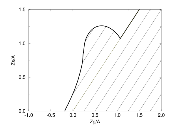
FIG. 6.: Values of $({\cal Z}_{S}/{\cal A},{\cal Z}_{P}/{\cal A})$, for which the sum rule (135) for $\left\langle\!\left\langle\sigma_{6}\right\rangle\!\right\rangle_{0}^{(N_{f}=3)}$ is positive for any positive scaling parameter $\zeta=V\Sigma^{2}/{\cal A}$ (the forbidden zone is hatched).

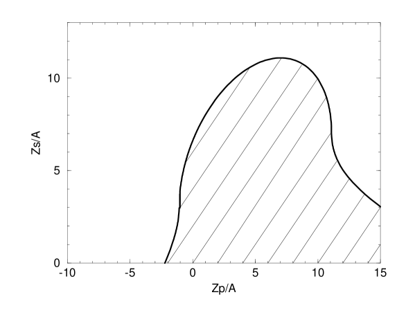
FIG. 7.: Values of $({\cal Z}_{S}/{\cal A},{\cal Z}_{P}/{\cal A})$ for which the sum rule (130) for $\left\langle\!\left\langle\sigma_{4}\right\rangle\!\right\rangle_{0}^{(N_{f}=10)}$ is positive for any positive scaling parameter $\zeta=V\Sigma^{2}/{\cal A}$ (the forbidden zone is hatched).

REFERENCES

- [1] L. Maiani, G. Pancheri and N. Paver Eds., The second DAPHNE physics handbook, Frascati, Italy: INFN (1995).
- [2] A.M. Bernstein, D. Drechsel and T. Walcher Eds., Chiral dynamics: Theory and experiment. Proceedings, Workshop, Mainz, Germany, September 1-5, 1997, Berlin, Germany: Springer (1998).
- [3] M. Baillargeon and P.J. Franzini, in Ref. [1], hep-ph/9407277. J. Lowe in Ref. [2], J. Schacher in id., hep-ph/9711361.
- [4] D.J. Gross and F. Wilczek, Phys. Rev. Lett. 30 (1973) 1343.
- [5] T. Banks and A. Zaks, Nucl. Phys. B196 (1982) 189.
- [6] E. Gardi and G. Grunberg, J. High Energy Phys. 03 (1999) 024, hep-th/9810192.
- [7] T. Appelquist, A. Ratnaweera, J. Terning and L.C. Wijewardhana, Phys. Rev. D58 (1998) 105017, hep-ph/9806472.
- [8] M. Velkovsky and E. Shuryak, Phys. Lett. B437 (1998) 398, hep-ph/9703345. T. Appelquist and S.B. Selipsky, Phys. Lett. B400 (1997) 364, hep-ph/9702404.
- [9] S. Descotes, L. Girlanda and J. Stern, hep-ph/9910537.
- [10] J. Schwinger, Phys. Rev. 93 (1954) 615. R. Schrader and R. Seiler, Comm. Math. Phys. 61 (1978) 169. H. Hogreve, R. Schrader and R. Seiler, Nucl. Phys. B142 (1978) 525. D. Brydges, J. Frohlich and E. Seiler, Ann. Phys. 121 (1979) 227. J.E. Avron and B. Simon, Phys. Lett. A75 (1980) 41.
- [11] C. Vafa and E. Witten, Commun. Math. Phys. 95 (1984) 257.
- [12] T. Banks and A. Casher, Nucl. Phys. B169 (1980) 103.
- [13] J. Stern, hep-ph/9801282.
- [14] J.J. Verbaarschot, hep-ph/9902394.
- [15] T. Schafer and E.V. Shuryak, Rev. Mod. Phys. 70 (1998) 323, hep-ph/9610451.
- [16] S. Spanier and N. Tornqvist in Eur. Phys. J. C3 (1998) 390. For a recent discussion, M.R. Pennington, hep-ph/9905241, and references therein.
- [17] I.I. Kogan, A. Kovner and M. Shifman, Phys. Rev. D59 (1999) 016001, hep-ph/9807286.
- [18] Y. Iwasaki, K. Kanaya, S. Kaya, S. Sakai and T. Yoshie, Prog. Theor. Phys. Suppl. 131 (1998) 415, hep-lat/9804005.
- [19] D. Chen and R.D. Mawhinney, Nucl. Phys. Proc. Suppl. 53 (1997) 216, hep-lat/9705029. R.D. Mawhinney, Nucl. Phys. Proc. Suppl. 60A (1998) 306, hep-lat/9705031. C. Sui, Nucl. Phys. Proc. Suppl. 73 (1999) 228, hep-lat/9811011.
- [20] B. Moussallam, Eur. Phys. J. C14 (2000) 111, hep-ph/9909292. B. Moussallam, hep-ph/0005245. S. Descotes and J. Stern, hep-ph/0007082.
- [21] H. Leutwyler and A. Smilga, Phys. Rev. D46 (1992) 5607.
- [22] J. Gasser and H. Leutwyler, Ann. Phys. 158 (1984) 142 ; Nucl. Phys. B250 (1985) 465.
- [23] N.H. Fuchs, H. Sazdjian and J. Stern, Phys. Lett. B269 (1991) 183; Phys. Rev. D47 (1993) 3814. M. Knecht and J. Stern, in Ref. [1], hep-ph/9411253. J. Stern, hep-ph/9712438. M. Knecht, B. Moussallam, J. Stern and N.H. Fuchs, Nucl. Phys. B457 (1995) 513.
- [24] J. Gasser and H. Leutwyler, Nucl. Phys. B307 (1988) 763.
- [25] C.G. Callan, R.F. Dashen and D.J. Gross, Phys. Lett. 63B (1976) 334. R. Jackiw and C. Rebbi, Phys. Rev. Lett. 37 (1976) 172.
- [26] G. ’t Hooft, Phys. Lett. B349, 491 (1995), hep-th/9411228.
- [27] J. Gasser and H. Leutwyler, Phys. Lett. 184B (1987) 83; Phys. Lett. 188B (1987) 477.
- [28] A. D. Jackson, M. K. Sener and J. J. Verbaarschot, Phys. Lett. B387 (1996) 355, hep-th/9605183.
- [29] J. Bijnens, G. Ecker and J. Gasser in Ref. [1], hep-ph/9411232.
- [30] P. Hasenfratz and H. Leutwyler, Nucl. Phys. B343 (1990) 241.
- [31] M. Gell-Mann, R.J. Oakes and B. Renner, Phys. Rev. 175 (1968) 2195.
- [32] A. Duncan, E. Eichten and H. Thacker, Phys. Rev. D59 (1999) 014505, hep-lat/9806020; Nucl. Phys. Proc. Suppl. 73 (1999) 837, hep-lat/9809144 and 840, hep-lat/9809117. A. Duncan, E. Eichten, R. Roskies and H. Thacker, Phys. Rev. D60 (1999) 054505, hep-lat/9902015.
- [33] E. Farhi and L. Susskind, Phys. Rept. 74 (1981) 277. M.E. Peskin and T. Takeuchi, Phys. Rev. D46 (1992) 381.
- [34] T. Appelquist, P.S. Rodrigues da Silva and F. Sannino, hep-ph/9906555. T. Appelquist, J. Terning and L.C. Wijewardhana, Phys. Rev. Lett. 79 (1997) 2767, hep-ph/9706238.
- [35] L. Girlanda and J. Stern, hep-ph/9906489. L. Ametller, J. Kambor, M. Knecht and P. Talavera, Phys. Rev. D60 (1999) 094003, hep-ph/9904452. L. Girlanda, PhD Thesis, Université Paris-XI, Orsay, France (1999).