Deep Inelastic Scattering, Diffraction and all that

Abstract

These lectures include an introduction to the partonic description of the proton, the photon and the ‘colour singlet’, as seen in inclusive and semi-inclusive DIS, in $e^{+}e^{-}$ collisions, and in diffractive processes, respectively. Their formal treatment using structure, fragmentation, and fracture functions is outlined giving an insight into the perturbative QCD framework for these functions. Examples and comparisons with experimental data from LEP, HERA, and Tevatron are also covered.

Introduction

The discovery of asymptotic freedom, one of the most significant properties of strong interactions embodied by Quantum Chromodynamics (QCD) opened, more than 25 years ago, a new chapter in our understanding of the structure of matter which has has been actively followed by theoreticians and experimentalists ever since. The short distance structure of hadrons, together with the production of jets in hadronic collisions are paradigmatic among the strong interaction phenomena successfully accounted by QCD and even though the standing of the theory is today well established, further theoretical refinements and the corresponding experimental validation renew constantly the original enthusiasm of the high energy physics community.

These lectures intend to provide an overview of the more recent topics of high energy collisions related in a way or another to perturbative QCD. First we briefly remind the essentials of QCD, including the main features of partons (the quarks and gluons), which are the true protagonists in the story. Then, we refer to what is known about the partonic structure of three of the main benchmarks of QCD, the proton, the photon, and the singlet colour or ’pomeron’. Finally we will try to draw the connections between their corresponding structures which in some way relate the physics made in the three main HEP laboratories.

As usual, many interesting and highly active topics have been excluded from the lectures in favor of a more detailed analysis of the covered points. These include, for example, those related to the spin structure of the proton, which have driven an ongoing series of polarized experiments and a great deal of theoretical discussions Lampe ; heavy flavours, which involve very subtle theoretical approaches, and perturbative QCD beyond NLO, which is relevant for the most recent high precision experiments BASS .

QCD

The strong interactions among quarks and gluons are described by Quantum Chromodynamics (QCD), the non-abelian gauge theory based on the gauge group $SU(3)_{C}$. Each quark flavour corresponds to a colour triplet in the fundamental representation of $SU(3)$ and the gauge fields needed to maintain the gauge symmetry, the gluons, are in the adjoint representation of dimension 8. Gauge invariance ensures that gluons are massless. The QCD Lagrangian may be written as

$${\cal{L}}_{QCD}=-\frac{1}{4}\,F^{a}_{\mu\nu}\,F^{\mu\nu}_{a}+\bar{\psi}_{i}\,(i\,\gamma^{\mu}\,D_{\mu}-m)\,\psi_{i}$$ (1)

where

$$F^{a}_{\mu\nu}=\partial_{\mu}G^{a}_{\nu}-\partial_{\nu}G^{a}_{\mu}+g\,f^{abc}\,G_{b\mu}\,G_{c\nu}$$ (2)

stands for the gluon field tensor, $\psi_{i}$ are the quark fields and the covariant derivative is defined by

$$D_{\mu}=\partial_{\mu}-i\,g\,T_{a}\,G^{a}_{\mu}$$

The strong coupling is represented by $g$ and indices are summed over $a=1,...,8$ and over $i=1,2,3$. Finally, $T_{a}=\lambda_{a}/2$ and $f_{abc}$ are the $SU(3)$ generators and structure constants, respectively, which are related by $[T_{a},T_{b}]=i\,f_{abc}\,T^{c}$.

Like in Quantum Electrodynamics (QED), the procedure employed to deal consistently with the divergences that occur in the computation of strong interactions beyond the tree level, shows that the actual strength of the QCD coupling depends on the energy scale of the process. But in opposition to QED, this renormalized strong coupling is small at high energy (momentum), going to zero logarithmically, i.e. QCD has the property of asymptotic freedom. Consequently, in this regime perturbation theory is valid and tests against experimental data can be performed in terms of hadrons. Figure 1 summarize the basic QCD perturbative processes appearing in different circumstances.

Figure 1: Basic processes in perturbative QCD.

Experiments with $e^{-}\,e^{+}$ colliders provide clean results for QCD tests. Recently, a huge amount of experimental data came from the HERA electron-proton collider revHE and also from the Tevatron at Fermilab revFE . In both cases, there is a hadronic remnant that make the analysis a little more involved. All this experimental evidence support the existence of quarks being colour triplets of spin $1/2$ and of gluons being vector octets. Moreover, the presence of the QCD coupling has manifested itself in different measurements, as well as the above mentioned property of asymptotic freedom. This information comes mainly from the study of the so called two- and three-jets events DIS .

When a given process needs a higher order in perturbation theory to be known, it is necessary to compute not only the renormalized strong coupling constant but also the appropriate corrections to the relevant cross-sections. As is usual in Quantum Field Theory, a regularization-renormalization procedure is in order, just to absorb divergences into the definition of physical quantities. This prescription requires the introduction of a new scale $\mu$, fixing the renormalization point, and all renormalized quantities begin to depend on it. Nevertheless, different prescriptions must end with the same predictions for observables.

In order to illustrate how the general procedure works, ending with the Renormalization Group equations that guarantee that physical observables do not depend on the scale $\mu$, let us show what happens with Green functions. Just to remember the procedure, let us begin with a single particle irreducible Green function $\Gamma$. In general, to control divergences, one has to introduce an ultra-violet cut-off $\Lambda$, or the equivalent dimensional regularization parameter, in the loop momentum integral defining the $\Gamma$. In a renormalizable theory, as QCD is, a renormalized Green function is defined as

$$\Gamma_{R}(p_{i},g,\mu)=Z_{\Gamma}(g_{0},\Lambda/\mu)\,\Gamma_{U}(p_{i},g_{0},\Lambda)$$

where $p_{i}$ stands for the external particle momenta, $g_{0}$ and $g$ are the bare and the renormalized couplings, respectively. This $\Gamma_{R}$ is then finite in the limit $\Lambda\rightarrow\infty$ but it depends on the scale at which the value of the renormalized quantities are fixed, the prescription parameter $\mu$. The function $Z_{\Gamma}$ is a product of renormalization factors. Due to the fact that the unrenormalized $\Gamma_{U}$ is obviously independent of $\mu$, one has to demand

$$\frac{d\Gamma_{U}}{d\mu}=0$$

and consequently, the Renormalization Group Equation (RGE)

$$\left(\mu\,\frac{\partial}{\partial\mu}+\beta\,\frac{\partial}{\partial g}+\gamma\right)\,\Gamma_{R}(p_{i},g,\mu)=0$$ (3)

has to be verified. Here $\gamma$ is the anomalous dimension, depending on the particular Green function under consideration, and the beta-function is universal

$$\gamma=\frac{\mu}{Z_{\Gamma}}\,\frac{\partial Z_{\Gamma}}{\partial\mu}\,\,\,\,\,\,\,\,\,\,\,\,\,\,\beta(g)=\mu\,\frac{\partial g}{\partial\mu}$$ (4)

If there is only one large momentum scale $Q$, or $Q^{2}$ as it is standard to quote, as it is the case here, one can express all $p_{i}$ in terms of a fixed fraction $x_{i}$ of $Q$. Then, defining the so called evolution variable

$$t=\frac{1}{2}\,\ln\left(\frac{Q^{2}}{\mu^{2}}\right)$$ (5)

it is possible to introduce the momentum dependent, or running coupling through the integral

$$t=\int^{g(t)}_{g(0)}\frac{dg^{\prime}}{\beta(g^{\prime})}$$

and the general solution of the RGE reads

$$\Gamma(t,g(0),x_{i})=\Gamma(0,g(t),x_{i})\,\,exp\left[\int^{g(t)}_{g(0)}dg^{\prime}\,\frac{\gamma(g^{\prime})}{\beta(g^{\prime})}\right]$$

This solution explicitly shows that the $Q$-scale dependence of $\Gamma$ arises entirely through the running coupling $g(t)$. Introducing now the usual notation

$$\alpha_{s}=\frac{g^{2}}{4\pi}$$ (6)

one can expand the beta-function in a power series in $\alpha_{s}$

$$\beta(\alpha_{s})=\mu\,\frac{\partial\alpha_{s}}{\partial\mu}=-\frac{\beta_{0}}{2\pi}\,\alpha^{2}_{s}-\frac{\beta_{1}}{4\pi^{2}}\,\alpha^{3}_{s}-...$$ (7)

where it results beta that

$$\beta_{0}=11-\frac{2}{3}\,N_{f}\,\,\,\,\,\,\,\,\,\,\beta_{1}=51-\frac{19}{3}\,N_{f}$$ (8)

Here $N_{f}$ indicates the number of flavours that can be excited (with mass less than $\mu$) at the scale $\mu$.

It is clear that the solution of the differential equation for $\alpha_{s}$ introduces a constant, called $\Lambda_{QCD}$, which has to be fixed by using experimental data. The resulting $\alpha_{s}$ can be written as

$$\alpha_{s}(\mu,\Lambda_{QCD})=\frac{4\,\pi}{\beta_{0}\,\ln(\mu^{2}/\Lambda_{QCD}^{2})}\,\left\{1-\frac{2\,\beta_{1}}{\beta_{0}^{2}}\,\frac{\ln[\ln(\mu^{2}/\Lambda_{QCD}^{2})]}{\ln(\mu^{2}/\Lambda_{QCD}^{2})}\right\}$$ (9)

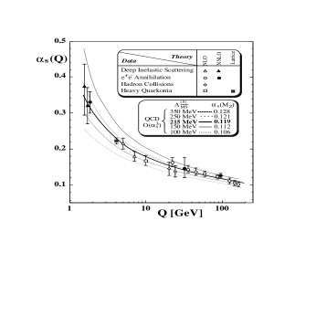
Figure 2: QCD running coupling.

This expression for the running coupling shows clearly the property of asymptotic freedom of QCD, i.e., the coupling vanishes when the scale becomes asymptotic, namely $\mu\rightarrow\infty$. Consequently, in this momentum regime, perturbation theory is valid.

A very clear quantitative test of perturbative QCD is provided by the measurement of $\alpha_{s}$ in different processes at different scales $Q^{2}$. In Figure 2 there is a summary of the various determinations of $\alpha_{s}$ 9810316 .

The present world average PDG for the coupling at the $Z^{0}$ mass is

$$\alpha_{s}(M_{Z})=0.119\pm 0.002$$

which implies

$$\Lambda_{QCD}^{\overline{MS}}=220+78-63\,MeV$$

corresponding to five flavours excited and in the conventional $\overline{MS}$ prescription commonly used.

Proton

Having reviewed the essentials of QCD, we now proceed with the analysis of one of the most rich benchmarks of perturbative QCD which is the short distance structure of the proton.

We start this section giving a set of definitions of the commonly used relativistic invariants related to Deep Inelastic Scattering, DIS, one of the fundamental experimental tools for hadron analysis, together with the corresponding formulae for the neutral and charged current cross-sections, where the structure functions are introduced. These functions will be latter expressed in terms of the quark-parton model including QCD corrections. For a more detailed treatment see DIS

Lorentz Invariants

Figure 3: DIS kinematics.

The scattering of a lepton from a proton (or in general a nucleon, a hadron or a nucleus), at high enough $Q^{2}$, can be viewed as the (elastic) scattering of the lepton from a quark or antiquark inside the proton mediated by the exchange of the corresponding virtual vector boson $\gamma^{\star},\,W^{\star}$ or $Z^{\star}$. Consequently, when the process is totally inclusive (one integrates over all final hadronic activity), can be fully described by two Lorentz invariants. With the momentum assignment of Figure 3 one can construct the following invariants:

$$s=(p+k)^{2},\,\,\,\,\,t=(p-p^{\prime})^{2},\,\,\,\,\,W^{2}=(p+q)^{2},\,\,\,\,\,Q^{2}=-(k^{\prime}-k)^{2}=-q^{2}$$ (10)

defined as the centre of mass energy squared, the square of the four-momentum transfer between the proton and the final hadronic state, the invariant mass squared of the final hadronic state, and four momentum transfer squared between the lepton and the proton, respectively. It is also convenient to introduce dimensionless invariants (scaling variables)

$$y=\frac{p\cdot q}{p\cdot k}\,\,\,\,\,,\,\,\,\,\,x=\frac{Q^{2}}{2\,p\cdot q}$$ (11)

i.e. the inelasticity of the scattered lepton, and fraction of the proton momentum carried by the struck quark, or Bjorken variable, respectively.

Notice finally that, ignoring masses,

$$Q^{2}=s\,x\,y\,\,\,\,\,\,\,\,\,\,W^{2}=Q^{2}\,\frac{1-x}{x}$$ (12)

so that $Q^{2}_{max}=s$, the center of mass energy squared, and small values of $x$ imply increasing $W$. As we have already said, in principle one is allowed to use any pair of these invariants to describe totally inclusive DIS. Usually $x$ and $Q^{2}$ are the preferred ones.

Another interesting point to remark concerns the resolving power of a DIS experiment. Clearly, the size $d$ one can resolve inside the nucleon becomes smaller for large photon, or gauge boson in general, virtuality, namely

$$d\sim\frac{\hbar\,c}{Q}\simeq 0.2\,\frac{GeV\,fm}{Q}$$

The ‘magnifying power’ is then $d\simeq 10^{-14}\,cm$ for $Q^{2}=4\,GeV^{2}$, and $d\simeq 10^{-16}\,cm$ and for $Q^{2}=40,000\,GeV^{2}$.

Experimental Reconstruction

Different DIS experiments cover different regions of the kinematical plane ($x,Q^{2}$) as shown in Figure 4 9712505 . It is particularly interesting the very extended range covered by HERA: $Q^{2}\simeq 0.2\,-\,10^{4}\,GeV^{2}$ and $x\simeq 10^{-5}\,-\,10^{-1}$.

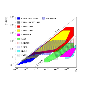
Figure 4: Coverage of the ($x,Q^{2}$) plane by the various DIS experiments

The kinematics of the DIS events, namely the two invariants required to specify DIS processes, can be determined (particularly at HERA) from measurements on the electron (the lepton) alone, on the final hadronic state corresponding to the struck quark alone or on a mixture of both. In general, the preferred method depends on the particular kinematical region of interest, strongly correlated with the detector performance.

The electron method: The input are the energy $E^{\prime}_{e}$ of the final electron and the electron scattering angle $\theta_{e}$ measured with respect to the proton beam direction ($\theta_{e}=180^{\circ}$ means zero electron scattering angle)

$$y_{e}=1-\frac{E^{\prime}_{e}}{E_{e}}\,\sin^{2}\frac{\theta_{e}}{2}\,\,\,\,\,\,\,\,\,\,Q^{2}_{e}=4\,E_{e}\,E^{\prime}_{e}\,\cos^{2}\frac{\theta_{e}}{2}$$

The hadron method: The input is the hadronic energy $E_{h}$ and the three-momentum components of the hadronic system. They are computed as the sum over all final state hadrons $h$

$$y_{h}=\frac{\sum_{h}(E_{h}-p_{z,h})}{2\,E_{e}}\,\,\,\,\,\,\,\,\,\,Q^{2}_{h}=\frac{p^{2}_{x,h}+p^{2}_{y,h}}{1-y_{h}}$$

This method is also known with the name Jacquet-Blondel, because these authors were able to show that the contribution from hadrons lost in the beam pipe is negligible.

The sigma method: This method is based on both electron and hadron measurements. The denominator of $y_{h}$ is replaced by a sum over all final state particles including the scattered electron (certainly equal to $2\,E_{e}$ due to energy-momentum conservation). The name of the method comes from the introduction of the variable $\Sigma=\sum_{h}(E_{h}-p_{z,h})$ that appears in

$$y_{\Sigma}=\frac{\Sigma}{\Sigma+E^{\prime}_{e}\,(1-\cos\theta_{e})}\,\,\,\,\,\,\,\,\,\,Q^{2}_{\Sigma}=\frac{E^{\prime 2}_{e}\,\sin^{2}\theta_{e})}{1-y_{\Sigma}}$$

Notice that the denominator in $y_{\Sigma}$ is twice the true incident electron energy in the eventual case when the electron radiates photons that are not detected.

There are other more sophisticated methods, well adapted to particular situations, like the so-called double angle method or the PT method used by ZEUS revHE .

Cross-sections

The fundamental measurement in DIS experiments concerns the totally inclusive cross-section for

$$\ell(k)+N(p)\rightarrow\ell^{\prime}(k^{\prime})+X(p^{\prime})$$

as a function of the kinematical variables defined above. For charged lepton-nucleon scattering mediated by the neutral current, the spin averaged cross-section is given in terms of the structure functions $F_{2}$, $F_{L}$ and $F_{3}$

$$\frac{d^{2}\sigma_{\pm}}{dx\,dQ^{2}} = \frac{4\,\pi\alpha^{2}}{x\,Q^{4}}$$

$$\left[\left(1-y+\frac{y^{2}}{2}\right)\,F_{2}(x,Q^{2})-\frac{y^{2}}{2}\,F_{L}(x,Q^{2})\mp\left(y-\frac{y^{2}}{2}\right)\,F_{3}(x,Q^{2})\right]$$

here $\alpha$ is the QED coupling constant. For $Q^{2}$ values below the $Z^{0}$ scale, the parity violating effects related to $F_{3}$ are negligible and all the process is due to $\gamma^{\star}$ exchange. Remember also that the longitudinal structure function $F_{L}$, a QCD correction important for large $y$, is defined in terms of the standard $F_{1}$ and $F_{2}$, related to the transverse and longitudinal $\gamma^{\star}\,N$ cross sections respectively, as

$$F_{L}(x,Q^{2})=F_{2}(x,Q^{2})\,\left(1+\frac{4\,M_{N}^{2}\,x^{2}}{Q^{2}}\right)-2\,x\,F_{1}(x,Q^{2})$$ (14)

and that in the naive quark-parton model, really valid at extremely high $Q^{2}$, where quarks are considered free, massless, having spin $1/2$ and without any $p_{T}$ developed, $F_{L}$ is zero because the Callan-Gross relation

$$2\,x\,F_{1}(x)=F_{2}(x)$$

is satisfied. Under this assumptions, the so called Bjorken scaling is fully satisfied, namely, structure functions are only function of the $x$ variable.

The ratio $R$ is defined by

$$R(x,Q^{2})=\frac{F_{L}(x,Q^{2})}{F_{2}(x,Q^{2})-F_{L}(x,Q^{2})}=\frac{\sigma_{L}}{\sigma_{T}}$$ (15)

which is obviously zero in the Callan-Gross limit and can be interpreted as the ratio of cross-sections for the absorption of transversely and longitudinally polarized virtual photons on nucleon. The differential cross-section (Cross-sections) can be rewritten in terms of $R(x,Q^{2})$ as

$$\frac{d^{2}\sigma}{dx\,dQ^{2}}=\frac{4\,\pi\alpha^{2}}{x\,Q^{4}}\left[1-y-\frac{M_{N}^{2}\,x^{2}\,y^{2}}{Q^{2}}+\frac{y^{2}}{2}\,\frac{1+\frac{4\,M_{N}^{2}\,x^{2}}{Q^{2}}}{1+R(x,Q^{2})}\right]\,F_{2}(x,Q^{2})$$ (16)

where the parity violating contribution was discarded.

It is possible to specify the structure function $F_{2}$ in terms of the partons (or better quarks) within the nucleon as follows

$$F_{2}(x,Q^{2})=x\,\sum_{f}\,e^{2}_{q_{f}}\,\left[q_{f}(x,Q^{2})+\bar{q}_{f}(x,Q^{2})\right]$$ (17)

where the sum runs over all momentum distributions of quarks of the different flavours $f$ excited ($x\,q_{f}(x,Q^{2})$) and antiquarks ($x\,\bar{q}_{f}(x,Q^{2})$) contained in the nucleon and $e_{q_{f}}$ stands for the the different parton-photon couplings, namely their electric charges. Notice that the previous expression (17) is valid only in leading order of perturbation theory. In fact, there one has included the explicit $Q^{2}$ dependence which is the effect of implementing first order perturbative QCD. However, there is a particular renormalization and factorization scheme that can be used in higher order QCD, the so called DIS-scheme, where one can retain that expression at any order of perturbation theory. In other schemes, like the usual $\overline{MS}$ one, the expressions for the structure functions are more involved, including in general $g(x,Q^{2})$, the gluon density in the nucleon.

Let us now refer for a moment to the inclusive reaction that goes via charged current

$$\nu_{\mu}+N\rightarrow\mu^{-}+X$$ (18)

where as usual we write $N$ for an isoscalar nucleon. In the QCD improved parton model, the corresponding cross section reads

$$\frac{d^{2}\sigma}{dx\,dy}=\frac{2\,G^{2}_{F}\,M_{N}\,E_{\nu}}{\pi}\,\left(\frac{M_{W}^{2}}{Q^{2}+M_{W}^{2}}\right)^{2}\,\left[x\,q(x,Q^{2})+x\,\bar{q}(x,Q^{2})\,(1-y^{2})\right]$$ (19)

$M_{W}$ stands for the charged intermediate boson mass. $G_{F}$ is the Fermi constant. The quark and antiquark distribution functions can be written in terms of the corresponding valence and sea flavour distributions in a proton as

$$2\,q(x,Q^{2}) = u_{v}(x,Q^{2})+d_{v}(x,Q^{2})+u_{s}(x,Q^{2})+d_{s}(x,Q^{2})$$

$$+2\,s_{s}(x,Q^{2})+2\,b_{s}(x,Q^{2})$$

$$2\,\bar{q}(x,Q^{2}) = u_{s}(x,Q^{2})+d_{s}(x,Q^{2})+2\,c_{s}(x,Q^{2})+2\,t_{s}(x,Q^{2})$$ (21)

One can introduce immediately the corresponding structure function $F_{2}$ for neutrino scattering. It is of interest to compare this $F_{2}^{\nu}$ with the one for charged lepton DIS written above. Taking into account the sea corrections, the relation between both $F_{2}$ functions results

$$\frac{F_{2}^{\ell}}{F_{2}^{\nu}}=\frac{5}{18}\,\left(1-\frac{3}{5}\,\frac{s+\bar{s}-c-\bar{c}}{q+\bar{q}}\right)$$ (22)

This relation compares well with experimental data chek .

QCD evolution equations

All the functions introduced above include an explicit $Q^{2}$ dependence. This fact reflects the presence of interactions among partons. Clearly, the parton model, that implies exact Bjorken scaling, has to be modified to include these interactions. Moreover, quarks and gluons are finally confined within hadrons by the non-Abelian gauge interaction in QCD. Even if QCD is with us for more than 25 years, it has not yet been possible to calculate in detail the structure of hadrons starting from quarks, gluons and their gauge interactions, making compatible the short distance almost free partons with the long distance confinement. This fact, related to the running character of the strong interaction strength that we have discussed above, is on the origin of our continuous use of structure (and fragmentation and fracture) functions in describing DIS. Fortunately enough, some factorization theorems, which are valid in QCD, allows one to split the problem into a perturbative part and a non-perturbative part. In other words, the cross-section can be expressed as the folding of the initial parton distribution function $q_{f/N}$, a non-perturbative input given the density of partons $f$ in the nucleon, with a lepton-parton cross-section that can be computed by means of perturbation theory inside QCD. This fact can be schematically written as

$$\sigma_{\ell N}=\sum_{f}q_{f/N}\,\otimes\,\sigma_{\ell q}$$

and consequently, it can be sketched as in Figure 5

Figure 5: Factorization in QCD

It is clear that the non-perturbative part, namely, the part related to structure functions, has to be determined by fitting experimental data. Nevertheless, they are universal in the sense that once obtained from a given particular process, they can be used in connection with any other one.

Regarding QCD as an improvement of the quark-parton model, we can say that the nucleon is not simply composed of three point-like quarks, the so called valence quarks but as soon as $Q^{2}$ increases, the vector boson ($\gamma^{\star}$, $Z^{\star}$ or $W^{\star}$) increasingly resolves the composition of the nucleon. One of the targets that the vector boson could find is one of the quarks, called sea quarks, which originate from a gluon, namely through

$$g\rightarrow q\,\bar{q}$$

being this gluon itself radiated from one of the valence quarks. In other words, increasing $Q^{2}$ means that the resolution of our “view” of the nucleon increases, so that the effective number of partons sharing the nucleon momentum also increases. Consequently, the probability of finding partons with small $x$ has increased while the corresponding one to large $x$ has decreased. This process clearly entails a violation of Bjorken scaling through a $Q^{2}$ dependence, that was born from QCD interactions. Consequently, to compare experimental data with QCD predictions. one has to compute perturbative QCD corrections to the fundamental process

$$V^{\star}\,q\rightarrow q$$ (23)

Nowadays, these corrections, even if the calculation is very involved, are well known up to order $\alpha_{s}^{2}$ Van . We give here only an introductory discussion of the lowest order corrections.

The relevant diagrams corresponding to the first terms of the perturbative expansion in $\alpha_{s}$ for the process (23) are presented in Figure 6 (We have omitted the vertex and self energy gluonic corrections, which are associated to the ultraviolet divergences. These are removed through coupling constant renormalization, and lead to the running coupling $\alpha_{s}(Q^{2})$ given in Equation (9))

Figure 6: Lowest QCD corrections to $V^{\star}\,q\rightarrow q$

Because we are considering the inclusive case, the calculation implies phase space integrations which lead to divergent integrals when partons become collinear. They have to be regularized by means of dimensional regularization Bol , a cut-off in the transverse momentum of the partons, or giving them masses. Any of these procedures introduce a regulator $\mu^{2}$ which has the dimension of the energy scale $Q^{2}$.

For example, to order $\alpha_{s}$, quarks contribute to the structure function $F_{2}$ through the following convolution integral

$$F^{quarks}_{2} (x,Q^{2})=$$ (24)

$$x\,\sum_{f,\overline{f}}e_{f}^{2}\,\int_{0}^{1}\frac{dy}{y}\,q_{f}(y)\left[\delta\left(1-\frac{x}{y}\right)+\frac{\alpha_{s}}{2\pi}\left\{P_{qq}\left(\frac{x}{y}\right)\,\ln\frac{Q^{2}}{\mu^{2}}+R\left(\frac{x}{y}\right)\right\}\right]$$

where $q_{f}(y)$ is the ‘bare’ quark density. The delta function term comes from the lowest order diagram in Figure 6, and represents the corresponding contribution to $F_{2}$ as in Equation (25). The first term between the curly brackets includes the factor $\ln(Q^{2}/\mu^{2})$ which diverges as the regulator $\mu^{2}$ goes to zero and is associated to the collinear gluon emission diagrams, while the second term collects the finite contributions from those diagrams. $P_{qq}(x/y)$ and $R(x/y)$ are known calculable functions.

The collinear singularities of course threaten the validity of the parton model, however they can be consistently removed from the partonic subprocess absorbing them into the ‘bare’ parton densities $q_{f}(y)$ defining renormalized parton densities

$$q_{f}(x,M^{2})=q_{f}(x)+\frac{\alpha_{s}}{2\pi}\int_{0}^{1}\frac{dy}{y}\,q_{f}(y)\left\{P_{qq}\left(\frac{x}{y}\right)\,\ln\frac{M^{2}}{\mu^{2}}+R^{\prime}\left(\frac{x}{y}\right)\right\}$$ (25)

where $M^{2}$ is factorization scale chosen to separate the short distance (‘partonic’) effects from the long distance (‘hadronic’) ones. For the parton model to make sense, the renormalized parton densities must be process independent, i.e. must be the same for DIS, Drell-Yan, and any other process. Fortunately, this proves to be the case to all orders of perturbation theory, and one ends up with an expression for the (physical, and thus finite) structure function $F_{2}(x,Q^{2})$ in terms of a finite renormalized parton density $q_{f}(x,M^{2})$ and an also finite partonic cross section

$$F^{quarks}_{2} (x,Q^{2})=$$ (26)

$$x\,\sum_{f,\overline{f}}e_{f}^{2}\,\int_{0}^{1}\frac{dy}{y}\,q_{f}(y,M^{2})\left[\delta\left(1-\frac{x}{y}\right)+\alpha_{s}\,C^{q}_{2}\left(\frac{x}{y},\frac{Q^{2}}{M^{2}}\right)\right]$$

At this point, it is customary to chose the factorization scale $M^{2}$ equal to the energy scale $Q^{2}$, factorizing the scale dependence of the cross sections into the parton densities.

The crucial observation here is that although perturbation theory can not make an absolute prediction for $q_{f}(x,Q^{2})$, from Equation (25) it follows

$$\frac{dq_{i}(x,M^{2})}{d{\rm log}Q^{2}} = \frac{\alpha_{s}}{2\pi}\int_{x}^{1}\frac{dy}{y}\left[q_{i}(y,Q^{2})\,P_{qq}\left(\frac{x}{y}\right)\right]$$ (27)

which means that QCD actually gives the $Q^{2}$ dependence of the parton distributions.

By means of a similar procedure with the gluon densities, one can deal with the divergences in the diagrams initiated by gluons. However, due to the possibility of gluons emitting quark pairs which then interact with the photon probe, the evolution the evolution of the quark and gluon densities is no longer independent, but coupled. Taking into account all the ${\cal{O}}(\alpha_{s})$ contributions, we end up with the so called DGLAP equations (or Altarelli-Parisi equations for short)

$$\frac{dq_{i}(x,Q^{2})}{d\ln Q^{2}} = \frac{\alpha_{s}}{2\pi}\int_{x}^{1}\frac{dy}{y}\left[q_{i}(y,Q^{2})\,P_{qq}\left(\frac{x}{y}\right)+g(y,Q^{2})\,P_{qg}\left(\frac{x}{y}\right)\right]$$

$$\frac{dg(x,Q^{2})}{d\ln Q^{2}} = \frac{\alpha_{s}}{2\pi}\int_{x}^{1}\frac{dy}{y}\left[\sum_{i}q_{i}(y,Q^{2})\,P_{gq}\left(\frac{x}{y}\right)+g(y,Q^{2})\,P_{gg}\left(\frac{x}{y}\right)\right]$$ (28)

Collecting all the ${\cal{O}}(\alpha_{s})$ contributions to $F_{2}(x,Q^{2})$, we finally arrive to the most usual expression for the structure function:

$$F_{2}(x,Q^{2}) = x\,\sum_{f}e_{f}^{2}\,C_{f}(x)\otimes\left[q_{f}(x,Q^{2})+\bar{q}_{f}(x,Q^{2})\right]$$

$$+C_{g}(x)\otimes g(x,Q^{2})$$

where $\otimes$ indicates a convolution integral and the index $g$ refers to gluons.

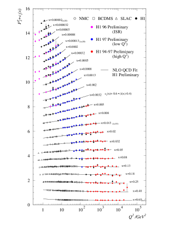
Figure 7: $F_{2}$ as a function of $Q^{2}$ and the corresponding QCD fit

Deep Inelastic Scattering (DIS) experiments and hadron-hadron interactions provide information on the parton structure of the nucleon and constraints the dynamics of the quark-gluon interaction given by QCD. In Figure 4 the kinematic regions in $x$ and $Q^{2}$ for cross section measurements in DIS $ep$ scattering, $\nu$ scattering and jets in $p\bar{p}$ collisions were presented. Data from the last years BASS have a clear influence on parton distributions and have motivated the update of parton distribution function analysis. Thes most recent sets are CTEQ5 CTEQ5 , GRV98 GRV98 and MRST MRST . The data playing a fundamental paper in these updates are the more precise ZEUS and H1 determinations of $F_{2}^{p}$ including $F_{2}^{charm}$; the NMC and CCFR final muon-nucleon and neutrino data; the E866 $pp$ and $pd$ lepton pair production asymmetry; the $W$ charge rapidity asymmetry; the D0 and CDF analysis of inclusive single jet production and the E706 direct photon production. It should be remarked that both approaches differ in the selection of data for the global analysis that are sensitive to gluons at large values of $x$. This means that a better understanding of the gluon behaviour at large $x$ is in order.

The $F_{2}$ structure function measurements at HERA cover a wide range of five orders of magnitude in both $x$ and $Q^{2}$ values as shown in Figure 4. One important point established by these data refers to the rise of the structure function with decreasing $x$. Moreover, QCD fits including NLO (next to leading order corrections) performed by the experimental collaborations are in very good agreement with the data even at low values of $Q^{2}\simeq 1\,GeV$. In Figure 7, $F_{2}$ is presented as a function of $Q^{2}$ for fixed values of $x$ from H1, ZEUS and the previous experiments, together with the QCD fit BASS .

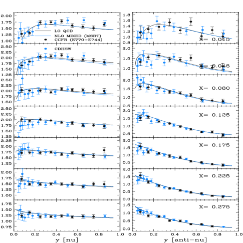
Figure 8: $\nu$ and $\bar{\nu}$ DIS as a function of $y$ from CCFR experiment together with QCD calculations

Figure 8 presents de neutrino and antineutrino cross section as a function of $y$ and different values of $x$ BASS . Data comes from the CCFR Fermilab experiment and is presented for $\langle E_{\nu}\rangle=150\,GeV$. A good agreement with previous data is observed and the NLO QCD analysis is satisfactory.

We finish this paragraph with a brief comment about some QCD technical details. The use of the renormalization group result for $\alpha_{s}$ in the AP approach, specifically the replacement of $\alpha_{s}$ by $\alpha_{s}(Q^{2})$ in Equation (28), has an important consequence. For each order of perturbation in $\alpha_{s}$ where the factorization procedure is performed, a whole series of perturbative contributions is efectively re-summed, in addition to the contributions comming form the corresponding diagrams shown in Figure 6. This kind of contributions are depicted in Figure 9, the so called ladder diagrams.

Figure 9: A typical ladder diagram

It can be shown that the improved AP approach takes into account contributions coming from the sum of all ladder diagrams in which the transverse momenta along the sides of the ladder are strongly ordered, namely: $Q_{0}^{2}\ll k_{T1}^{2}\ll\cdots\ll k^{2}_{Ti}\ll\cdots\ll Q^{2}$. This condition, of course implies also a strong ordering for the momenta of the emitted partons.

Notice that the calculation of such a n-th order ladder diagram implies integrations over the internal momenta. This nested integration can be carried out because of the $k_{T}$ ordering imposed, giving rise to results proportional to powers of $\alpha_{s}(Q^{2})$ and $\ln\left(Q^{2}/Q_{0}^{2}\right)$.

Now, it is clear that large logarithms in $Q^{2}$ compensate the small values of $\alpha_{s}(Q^{2})$, that as we have seen, decreases logarithmically. Consequently, all graph with rungs up to $n\rightarrow\infty$ would have to be summed up. The so called leading log approximation (LO), which is equivalent to follow the renormalization group improved AP approach up to order $\alpha_{s}$, collects all the contributions proportional to

$$\alpha_{s}^{n}(Q^{2})\,\left[\ln\left(\frac{Q^{2}}{Q_{0}^{2}}\right)\right]^{n}$$

while the next to leading log approximation (NLO), equivalent to the second order extension of the AP approach, also includes contributions proportional to

$$\alpha_{s}^{n}(Q^{2})\,\left[\ln\left(\frac{Q^{2}}{Q_{0}^{2}}\right)\right]^{n-1}$$

The AP approximation is expected to be valid for $Q^{2}$ values sufficiently large but also for $x$ not too small, just to ensure that small values of $x$ do not give rise to other large logarithms. In other words,

$$\alpha_{s}(Q^{2})\,\ln\left(\frac{1}{x}\right)\ll\alpha_{s}(Q^{2})\,\ln\left(\frac{Q^{2}}{Q^{2}_{0}}\right)<1$$

In is worth remarking that the AP equations can be solved analytically when a strong ordering in $x$ is also requiered. In this way one ends with the double leading log approximation, (DLL), where the large logarithmic terms are of the form Martin

$$\alpha_{s}^{n}(Q^{2})\,\left[\ln\left(\frac{Q^{2}}{Q_{0}^{2}}\right)\,\ln\left(\frac{1}{x}\right)\right]^{n}$$

This approximation is expected to be valid for large $Q^{2}$ and small $x$.

At small values of $x$, the parton content of the proton is gluon dominated. In this case the AP DLL can be obtained with the result

$$x\,g(x,Q^{2})\approx x\,g_{0}(x,Q_{0}^{2})\,exp\sqrt{\frac{144}{25}\,\ln\left[\frac{\ln(Q^{2}/\Lambda^{2})}{\ln(Q_{0}^{2}/\Lambda^{2})}\right]\,\ln(1/x)}$$ (30)

that shows that the gluon density increases faster than a power of $\ln(1/x)$.

In some cases of interest, $x$ is small enough but $Q^{2}$ is not sufficiently large to be inside the DLL regime. Under these circumstances, the AP approximation is not more valid. The BFKL (Balitsky, Fadin, Kuraev, Lipatov) equation has been proposed to tackle the limit behaviour of large $1/x$ and $Q^{2}$ finite and fixed. In this scheme, the $x_{i}$ variables in the ladder are stongly ordered, namely: $x_{0}\ll x_{1}\ll\cdots\ll x_{i}\ll\cdots\ll x$; while there is no order on $k_{T}$ imposed. This approach ends with the so called leading log approximation in $\ln(1/x)$. The region of validity being

$$\alpha_{s}(Q^{2})\,\ln\left(\frac{Q^{2}}{Q_{0}^{2}}\right)\ll\alpha_{s}(Q^{2})\,\ln\left(\frac{1}{x}\right)<1$$

Due to technical reasons, the BFKL equation is written in terms of the function $f(x,k_{T}^{2})$, related to the usual gluon density $g(x,Q^{2})$ that dominates at very small $x$ by

$$x\,g(x,Q^{2})=\int^{Q^{2}}_{0}dk_{T}^{2}\,\frac{f(x,k_{T}^{2})}{k_{T}^{2}}$$ (31)

The standard form of the equation is

$$\frac{\partial f(x,k_{T}^{2})}{\partial\ln(1/x)}=\frac{3\,\alpha_{s}}{\pi}\,k_{T}^{2}\,\int_{0}^{\infty}\frac{dk^{\prime 2}_{T}}{k_{T}^{\prime 2}}\,\left[\frac{f(x,k_{T}^{\prime 2})-f(x,k_{T}^{2})}{|k^{\prime 2}_{T}-k^{2}_{T}|}+\frac{f(x,k_{T}^{2})}{\sqrt{4\,k^{\prime 4}_{T}+k_{T}^{4}}}\right]$$ (32)

This approximate BFKL equation can be solved analytically for fixed $\alpha_{s}$. The solution behaves like

$$f(x,k_{T}^{2})\propto\left(\frac{x}{x_{0}}\right)^{-\lambda}$$

with

$$\lambda=\frac{N_{c}\,\alpha_{s}}{\pi}\,4\,\ln 2\approx 0.5$$ (33)

for $N_{c}=3$ and $\alpha_{s}=0.19$.

Consequently, the gluon density rises like a power of $1/x$ for decreasing $x$, namely

$$x\,g(x,Q^{2})\propto x^{-\lambda}$$

clearly faster than the AP DLL prediction (30). It should be noticed that a running $\alpha_{s}$ and higher order corrections decrease the value of $\lambda$.

Figure 10: $\lambda_{eff}$ and $dF_{2}/d\mbox{ln}Q^{2}$.

Assuming that gluons dominate at low $x$ one can expect an approximate behaviour for the structure function given by

$$F_{2}(x,Q^{2})\mid_{Q^{2}}=c\,x^{-\lambda_{eff}}\mid_{Q^{2}}$$

Figure 10 (a) shows the values obtained for $\lambda_{eff}$ as a function of $Q^{2}$ from fits to ZEUS and E665 data. Figure 10 (b) shows $dF_{2}/d\mbox{ln}Q^{2}$ as a function of $x$ 9812029 . In both figures QCD and Regge inspired fits have been included. The schematic map of the plane $\ln(Q^{2}),\ln(1/x)$ shown in Figure 11 intents to divide the regions where each of the two approaches, DGLAP and BFKL, are in order 9712505 .

Figure 11: The schematic map of the plane $\ln(Q^{2}),\ln(1/x)$

In the figure, a saturation region is indicated, where one waits the gluon density to be so high as to prevent its continuous growing.

Semi-inclusive

In the analysis of hadron structure, more information can be obtained if one goes one step beyond totally inclusive DIS, namely to semi-inclusive DIS, where one of the final hadrons is also measured

$$\ell+h\rightarrow\ell^{\prime}+h^{\prime}+X$$

In describing semi-inclusive processes, in addition to quark distributions, the so called fragmentation functions are necesary. These functions FEY describe, or better parametrize, a given parton decay into a final hadron.

It is clear that, in principle, the best process to analyze fragmentation functions is the semi-inclusive $e^{+}\,e^{-}$ annihilation, when a single hadron is fully detected in the final state

$$e^{+}\,e^{-}\rightarrow h(P)+X$$

The corresponding kinematics is depicted in Figure 12.

Figure 12: Schematic view of semi-inclusive $e^{+}\,e_{-}$

The relevant variables for this case are

$$z=\frac{2\,P\,q}{Q^{2}}\,\,\,\,\mbox{and}\,\,\,\,\tilde{z}=\frac{2\,p\,q}{Q^{2}}$$ (34)

It is also convenient to introduce $\zeta$ that measures the fraction of the parton momentum carried by the final hadron. The corresponding cross section reads

$$\frac{d\,\sigma_{h}(z,Q^{2})}{dz\,dQ^{2}} = \frac{4\,\pi\,\alpha^{2}}{Q^{2}}\sum_{i}\int d\tilde{z}\,\int d\zeta\,\delta(z-\tilde{z}\,\zeta)\,\tilde{\sigma}^{i}_{p}(\tilde{z},Q^{2})\,\zeta\,D^{h}_{i}(\zeta,Q^{2})$$

$$= \sum_{i}\int_{z}^{1}\frac{d\zeta}{\zeta}\,\tilde{\sigma}^{i}_{p}\left(\frac{\tilde{z}}{\zeta},Q^{2}\right)\,\zeta\,D^{h}_{i}(\zeta,Q^{2})$$

Here $\tilde{\sigma}^{i}_{p}$ is the parton $i$ production cross-section, that in the parton model results

$$\tilde{\sigma}^{i}_{p}(\tilde{z},Q^{2})=e_{i}^{2}\,\delta(1-\tilde{z})$$ (36)

if $i=q,\,\bar{q}$ and vanishes if $i=g$. The function $D^{h}_{i}(\zeta,Q^{2})$ is the fragmentation function or probability for a parton $i$ to decay into a hadron $h$ carrying the fraction $\zeta$ of the parton momentum.

When QCD corrections are in order, the fragmentation functions acquire a $Q^{2}$ dependence. The evolution of these functions with the scale

$$t=\ln\left(\frac{Q^{2}}{\mu^{2}}\right)$$ (37)

is given by the AP-like integrodifferential equations

$$\frac{dD^{h}_{q}}{dt}(z,t) = \frac{\alpha_{s}(Q^{2})}{2\,\pi}\,\int_{z}^{1}\frac{dy}{y}\,\left[D^{h}_{q}{dt}(y,t)\,P_{qq}(z/y)+2\,f\,D^{h}_{g}{dt}(y,t)\,P_{gq}(z/y)\right]$$ (38)

$$\frac{dD^{h}_{g}}{dt}(z,t) = \frac{\alpha_{s}(Q^{2})}{2\,\pi}\,\int_{z}^{1}\frac{dy}{y}\,\left[D^{h}_{q}{dt}(y,t)\,P_{qg}(z/y)+D^{h}_{g}{dt}(y,t)\,P_{gg}(z/y)\right]$$ (39)

The functions $P_{ij}$ are exactly the same as those appearing in the AP equations for the structure functions (28). The corresponding graphical interpretation in terms of the basic QCD processes is included in Figure 13.

Figure 13: QCD processes providing the evolution of fragmentation functions

It is worth noticing that the properties of the splitting functions are enough to guarantee the momentum sum rule

$$\sum_{h}\,\int_{0}^{1}z\,D^{h}_{q}(z,Q^{2})=1$$ (40)

and the analogous one for the gluon fragmentation function.

To solve the AP equations it is necessary to know the fragmentation functions at some value $Q^{2}_{0}$. Exactly as in the case of structure functions, they have to be obtained from experimental data. In general one proposes a given form for the initial $D$-function, in agreement with data, and then AP equations provide the evolution with $Q^{2}$.

Fracture Functions

For those who are not acquainted with fracture functions, let us briefly summarize that the main idea behind fracture functions is the realization that the most familiar perturbative description for semi-inclusive processes, based on parton distributions and fragmentation functions is, at least, incomplete VEN .

In the usual approach to semi-inclusive DIS, the corresponding cross section is expressed by a convolution between parton distributions and fragmentation functions accounting the process in which the struck parton hadronizes into a detected final state particle.

$$\frac{d^{3}\sigma_{curr.}}{dx\,dy\,dz}\simeq\frac{4\pi\alpha^{2}}{x\,(p+k)^{2}}\frac{1+(1-y)^{2}}{2y^{2}}\sum_{i}e^{2}_{i}\,q_{i}(x,Q^{2})\times D^{h}_{i}(z,Q^{2})$$ (41)

Obviously, this approach only takes into account hadrons produced in the current fragmentation region, and what is more, within this approximation, and in leading order, hadrons can only be produced in the backward direction. Going to higher orders one finds a breakdown of hard factorization, as there are collinear singularities that can not be substracted in the parton distributions or in the fragmentation functions.

All this means that there are additional contributions missing, which are mainly target fragmentation processes and are included in the so called fracture functions $M_{i}^{h}$, defined by

$$\frac{d^{3}\sigma_{targ.}}{dx\,dy\,dz}\simeq\frac{4\pi\alpha^{2}}{x\,(p+k)^{2}}\frac{1+(1-y)^{2}}{2y^{2}}\sum_{i}e^{2}_{i}\,(1-x)\,M^{h}_{i}(x,z,Q^{2})$$ (42)

These functions, that can be thought as the probabilities to find a parton of a given flavour in an already fragmentated target, straightforwardly solve the factorization problem and also allow a LO description of hadrons produced in the forward direction. The only subtlety regarding them is that they obey slightly different evolution equations; their scale dependence not only depends on their shape at a given scale but also on that of ordinary structure functions and fragmentation functions, reflecting the fact that current and target fragmentation are not truly independent of each other. This is usually refered to as ‘non homogeneus’ evolution

$$\frac{\partial M^{h}_{i}(x,z,Q^{2})}{\partial\mbox{ln}Q^{2}}=\frac{\alpha_{s}(Q^{2})}{2\pi}\int\frac{dy}{y}P_{ij}(y)M^{h}_{j}(\frac{x}{y},z,Q^{2})$$ (43)

$$+\frac{\alpha_{s}(Q^{2})}{2\pi}\int\frac{dy}{x(1-y)}\hat{P}_{ijl}(y)q_{j}(\frac{x}{y},Q^{2})D^{h}_{l}(\frac{zy}{x(1-y)},Q^{2})$$

As for structure functions in totally inclusive deep inelastic scattering, QCD does not predict the shape of fracture functions unless it is known at a given initial scale. This nonperturbative information have to be obtained from the experiment, and, eventually, can be parametrized finding inspiration in nonperturbative models, as it is the case for ordinary structure and fragmentation functions.

Fracture functions have been succesfully applied to the description of leading baryon production LB , have been extended to spin dependent processes FRACPOL , and as we shall see, are relevant for the description of diffractive DIS.

Photon

It may seem strange that the next step in our study of parton structure relies in a particle, the photon, that it is not a hadron and of course has no structure by itself, as we very well know. However, a high energy photon can ‘develop’ structure when interacting with another object. In fact, as the electromagnetic field couples to all particles carrying the electromagnetic current, a photon can fluctuate into particle-antiparticle virtual states, particularly into quark-antiquark pairs or even more complex hadronic objects with the same quantum numbers. As long a the fluctuation time is longer than the interaction time we can talk about the structure of the the photon, and deal with it as a ‘very special’ hadron. Notice that at high energies, the fluctuation of a photon into a state of invariant mass $M$ can persist for a time of the order of $\tau\sim 2\,E_{\gamma}/M$ until the virtual state materializes by a collision or annihilation with another system BRZ .

Figure 14: Photon Structure.

There are many reasons for this peculiar hadronic structure to be considered ‘matter’ of study. First of all, it gives the opportunity to study how QCD works in a completely different scenario. Theoretical studies of photonic parton distributions of real, i.e. on shell, photons have a long history initiated by Witten’s work witten . This description have been well established through measurements in $\gamma\gamma$ collisions at $e^{+}e^{-}$ colliders (PETRA, PEP, LEP) however, extending the idea of photon structure to high virtualities as in $ep$ processes like dijet production, a new insight has been gained as we link DIS, photoproduction, and $\gamma\gamma$ interactions Fer .

The concept of photon structure functions for real and virtual photons can be defined and understood in close analogy to deep inelastic lepton nucleon scattering, via the subproccess $\gamma^{*}(Q^{2})\gamma(P^{2})\longrightarrow X$ in $e^{+}e^{-}\longrightarrow e^{\pm}X$ as in Figure 14, where we denote the probed target photon with virtuality $P^{2}=-p^{2}_{\gamma}$ by $\gamma(P^{2})$ and reserve $\gamma^{*}(Q^{2})$ for the highly virtual one. The relevant differential cross section can be expressed, as in the hadronic case, in terms of the usual scaling variables $x$ and $y$ as

$$\frac{d^{2}\sigma(e\gamma(P^{2})\longrightarrow eX)}{dxdy} = \frac{2\,\pi\,\alpha^{2}\,s_{e\gamma}}{Q^{4}}\left[(1+(1-y)^{2})F_{2}^{\gamma(P^{2})}(x,Q^{2})\right.$$

$$\left.-y^{2}F_{L}^{\gamma(P^{2})}(x,Q^{2})\right]$$

with $F_{2,L}^{\gamma(P^{2})}(x,Q^{2})$ denoting the photonic structure functions. The measured $e^{+}e^{-}$ cross section is obtained by convoluting Equation(Photon) with the photon flux for the target photon $\gamma(P^{2})$ wei . The range of photon virtualities explored in the above mentioned experiment is given by

$$m_{e}^{2}\,y^{2}/(1-y)\leq P^{2}_{min}\leq P^{2}\leq P^{2}_{max}\leq\frac{s_{e\gamma}}{2}(1-y)(1-\cos\theta_{max})$$ (45)

where $m_{e}$ is the mass of the electron, $s_{e\gamma}$ is the square of the c.m.s. energy, $y$ is the energy fraction taken by the photon, and $\theta_{max}$ is the maximum scattering angle of the electron in the c.m.s. frame. $P^{2}_{min,max}$ are further determined by detector specifications and experimental settings.

Figure 15: Direct (a) and Resolved (b) Contributions to $F_{2,L}^{\gamma(P^{2})}(x,Q^{2})$.

It is worthwhile noticing that if one could neglect photon fluctuations into complex hadronic states, then the dependence of $F_{2,L}^{\gamma(P^{2})}(x,Q^{2})$ in both $x$ and $Q^{2}$ would be fully predictable in perturbative QCD. The pointlike process $\gamma^{*}(Q^{2})\gamma(P^{2})\longrightarrow q\bar{q}$, corrected by gluon radiation effects, yields a definite prediction for $F_{2,L}^{\gamma(P^{2})}(x,Q^{2})$. However, as it was anticipated, this is only the so called ‘direct’ contribution to the total process, named in opposition to the ‘resolved’ one, where the virtual photon $\gamma^{*}(Q^{2})$ strikes the nonperturbative ‘dressing’ of the photon fluctuation (Fig.15).

Figure 16: $F_{2}^{\gamma}(x,Q^{2})$ as a function of $Q^{2}$.

QCD corrections to the ‘direct’ component not only take into account the splitting of partons into partons as in the ordinary AP evolution equations, but also the possibility of a photon to split into a quark-antiquark pair. This implies an inhomogeneous term in the evolution equations and leads to a logarithmic enhancement in $F_{2,L}^{\gamma(P^{2})}(x,Q^{2})$ which means positive scaling violations for all values of $x$ (Fig.16) 9812030b .

The ‘resolved’ component obeys the same evolution equations typical of the lepton-hadron interactions. In a Vector Meson Dominance approach for the photon fluctuations, the resolved component is expected to vanish like $(1/P^{2})^{2}$ in connection to the vector meson propagator, however it is not clear up to which values of $P^{2}$ the nonperturbative contributions are relevant. In recent years several sets of parton distributions for real and virtual photons have been proposed glu ; phpd . For virtual photons, different approaches have been followed in LO y NLO global fits to the available LEP data (Figure 17) 9812030b .

Figure 17: $F_{2}^{\gamma}(x,Q^{2})$ as a function of $x$.

LEP data constraint reasonably well the quark distributions in the photon, however, in order to constrain the gluon densitiy it is much more suitable to analyze dijet production processes in $e^{+}\,p$ collisions as measured at HERA. As we shall see, in this context the picture of ‘direct’ and ‘resolved’ is also more clearly illustrated. In this kind of process the parton content of the proton is used to probe the iqi partonic structure of the photon as in a hadron-hadron collision. The hard scale invoked to allow such inspection and guarantee the validity of a perturbative treatment, is the large transverse momentum of the final state jets. Figure 18 depicts LO ‘direct’ and ‘resolved’ contributions to dijet production $e^{+}\,p$ collisions. As it can be seen, even at the lowest order, photonic gluons contribute to the cross section, at variance with what happens in $e^{+}e^{-}$ collisions.

Figure 18: Direct (a) and Resolved (b) Contributions to dijet production.

In leading order the differential cross section for two jet production in $ep$ collisions takes a very simple form when written in terms of the fraction of the photon energy intervening in the hard process, $x_{\gamma}$, the fraction of the proton energy carried by the participating parton, $x_{p}$, and that of the electron carried by the photon, $z$ DG0

$$\frac{d\sigma}{dx_{\gamma}\,dx_{p}\,dz\,dp_{T}\,dP^{2}}=\tilde{f}_{\gamma/e}(z,P^{2})\,q^{\gamma}(x_{\gamma},Q^{2},P^{2})\,q^{p}(x_{p},Q^{2})\,\frac{d\hat{\sigma}}{dp_{T}}$$ (46)

Here, $p_{T}$ is the transverse momentum of the jets, $P^{2}$ is the photon virtuality, and $Q^{2}$ is the relevant energy scale of the proccess, taken in this case equal to $p_{T}^{2}$. $d\hat{\sigma}/dp_{T}$ represents the hard parton-parton and parton-photon cross sections com .

The functions $q^{\gamma}(x_{\gamma},Q^{2},P^{2})$ and $q^{p}(x_{p},Q^{2})$ denote the parton distribution functions for the photon and the proton, respectively. The first one reduces to $\delta(1-x_{\gamma})$ -the probability for finding a photon in a photon- for direct contributions, i.e. those in which the photon participates as such in the hard process. $\tilde{f}_{\gamma/e}(z,P^{2})$ is the unintegrated Weizsäcker-Williams distribution man

$$\tilde{f}_{\gamma/e}(z,P^{2})=\frac{\alpha}{2\pi}\frac{1}{P^{2}}\frac{1+(1-z)^{2}}{z}$$ (47)

which has been shown to be a very good approximation for the distribution of photons in the electron, provided the photon virtuality is much smaller than the relevant energy scale glu .

Figure 19: a) Event distribution measured in dijet photoproduction. b) Ratio of ‘direct’ and ‘resolved’ photon cross sections as a function of the photon virtuality.

The differential cross section in Equation(46) can also be written in terms of the parton pseudorapidities $\eta_{1}$ and $\eta_{2}$, which are constrained by the experimental settings, and the electron and proton energies $E_{e}$ and $E_{p}$ kram . Both pairs of variables are related to the energy fractions by

$$x_{p}=\frac{p_{T}}{2E_{p}}\left(e^{\eta_{1}}+e^{\eta_{2}}\right)\,\,\,\,\,\,\,\,x_{\gamma}=\frac{p_{T}}{2zE_{e}}\left(e^{-\eta_{1}}+e^{-\eta_{2}}\right)$$ (48)

Kinematical restrictions constrain $x_{\gamma}$ to lay in the interval $[p_{T}^{2}/(x_{p}zE_{e}E_{p}),x_{\gamma}^{max}]$ , $x_{p}$ in $[p_{T}^{2}/(zE_{e}E_{p}x_{\gamma}^{max}),1]$ and $z$ in $[p_{T}^{2}/(E_{e}E_{p}),1]$.

Figure 20: Dijet cross sections for $Q^{2}<0.01GeV^{2}$ as a function of $x_{\gamma}$.

In the lowest order of QCD the ‘direct’ contribution is characterized by $x_{\gamma}=1$, which means that all the energy of the photon participates in the hard interaction. Allowing gluon corrections, ‘direct’ contributions may come from $x_{\gamma}\neq 1$, however one should expect them concentrated arround a peak at high $x_{\gamma}$. Conversely, ‘resolved’ contributions should be more copious al low $x_{\gamma}$ as for ordinary hadrons. In fact, this trend is shown by the measurements, as can be seen in Figure 19a 54levy . The variable $x_{\gamma}^{obs}$ used there to approximate $x_{\gamma}$ is the jet level equivalent of Equation (48)

$$x_{\gamma}^{obs}=\frac{p_{T}^{(1)}\,e^{-\eta_{1}}+p_{T}^{(2)}\,e^{-\eta_{2}}}{2zE_{e}}$$ (49)

where $p_{T}^{(i)}$ and $\eta_{i}$ refer to the transverse energies and pseudorapidities of the measured jets instead of those of the partons. Of course, the relative abundance of ‘direct’ and ‘resolved’ events depends strongly on the virtuality of the photon as can be seen in Figure 19b in accordance to the expectation about the suppression of the ‘resolved’ component as the virtuality increases 54levy .

Finally, it is quite instructive to anlyze the relative abundance of quark and gluon initiated contributions as a function of $x_{\gamma}$ in a typical $e^{+}p$ dijet cross section. In Figure 20 data obtained by H1 is compared to theoretical expectations based on a Montecarlo analysis using GRV parton distribution for the photon glu and for the proton GRV ; 9812030 . Notice that at large $x_{\gamma}$ the ‘resolved’ component is clearly dominated by quarks, however as $x_{\gamma}$ decreases, the photonic gluons become dominant.

Colour Singlet (Pomeron?)

In this section we draw our attention to a much more unfamiliar object, at least for the younger generation of physicists, although for some of us it may be an old acquaintance. We are talking about the pomeron, or in more modern language, about the colour singlet object which is exchanged when particles undergo strong interactions while preserving its nature. The possibility of studying the partonic structure of this old friend has been made real by a very recent generation of experiments and has added an extra quota of excitement in perturbative QCD.

Before we plunge ourselves into the partonic structure of the pomeron, it would be very helpful to first fetch some of the tools used in past to sail in those waters.

Peripheral model

Before the advent of QCD, the presence of structures in the differential cross-sections was mainly explained by means of dynamical exchange mechanisms like in the so called peripheral model. In this approach it is found that there is a clear enhancement near the forward direction whenever the crossed channel of the reaction has the quantum numbers of a known particle. Then, peripheralism proposes to express the scattering amplitude as a sum of contributions corresponding to the exchange of a particle. Namely

$$F=F_{\pi}+F_{V}+F_{B}+...$$

with

$$F_{i}\propto\frac{1}{m_{i}^{2}-t}$$

where it is clear that for small, physical (negative), values of $t$, there are peaks in the corresponding cross-section in s-channel, proportional to $|F|^{2}$. The indices $\pi,V,...$ represent pions, vector bosons, etc., and their masses hierarchize each contribution. The explanation of peripheral events cannot be found in QCD, since the exchanged particle is not a gauge boson that can be treated perturbatively. In fact the particles involved are composite objects such mesons or baryons.

When the exchanged particle has a spin $J$, the previous expression for the amplitude has to be replaced by

$$F_{i}\propto\frac{P_{J}(\cos\theta_{t})}{m_{i}^{2}-t}$$

and, if one remembers that the scattering angle in the $t$-channel reads

$$\cos\theta_{t}=1+\frac{2\,s}{t-4\,m^{2}}$$

it is found that the numerator of $F_{i}$ behaves asymptotically as $s^{J}$ for fixed $t$. This is not tenable because the Froissart bound is not satisfied for $J>1$. Moreover, that expression is purely real and does not satisfy the principle of analyticity.

There is a way out of the above mentioned difficulties, while maintaining the spirit of an exchange mechanism, now of an entire family of related particles. This proposal is based on the Regge poles ideas. These ideas emerge naturally in potential scattering theory through the analyticity properties of the amplitude. The Regge pole model REG is based then, upon the assumption of the following behaviour for the scattering amplitude

$$\lim_{s\rightarrow\infty\,,\,fixed\,t}\,F(s,t)\simeq\sum_{i}\beta_{i}(t)\,\frac{1+\xi_{i}\,e^{-i\,\pi\,\alpha_{i}(t)}}{\sin[\pi\,\alpha_{i}(t)]}\,\left(\frac{s}{s_{0}}\right)^{\alpha_{i}(t)}$$ (50)

here $\xi_{i}=\pm 1$ is called the signature of the corresponding Regge pole. The functions $\alpha_{i}(t)$ are called Regge trajectories and $\beta_{i}(t)$ residues of the poles that in general factorize between the initial and the final channels. Both functions $\alpha_{i}(t)$ and $\beta_{i}(t)$ are analytic functions of $t$.

The high energy model so introduced is understood as an exchange model where the Regge trajectories $\alpha_{i}(t)$ are such that they pass through the spin values of the particles, or better the resonances, each time positive $t$ takes the values of their mass squared. In this way, the collective effect of the exchange of all members of the family is taken into account. Clearly, the Froissart bound (total cross-sections cannot increase faster than $\ln^{2}\,s$) is satisfied as soon as

$$\alpha_{i}(t\leq 0)\leq 1$$

in the space-like region of negative $t$, relevant for the sacttering process.

Let us take as an example the case of pion-nucleon charge-exchange

$$\pi^{-}\,\,p\rightarrow\pi^{0}\,\,n$$

that has always been the paradigmatic case of reggeology. The $t$-channel of this reaction is

$$\pi^{-}\,\,\pi^{0}\rightarrow\bar{p}\,\,n$$

having the quantum numbers; $Q=1$, $I=1$, $Y=0$. $G=+1$ that correspond to the well known meson resonances $\rho\,(770\,MeV)$ of spin 1 and $g\,(1680\,MeV)$ of spin 3. This sequence of resonances defines precisely the meson Regge trajectory of isospin $1$, G-parity $+1$ and positive signature that is noted $\alpha_{\rho}$. The continuation of this trajectory to negative $t$ values, takes us into the physical region corresponding to the $s$-channel charge-exchange reaction. The parameters of a standard linear trajectory are the intercept at $t=0$ and the slope. In the present case, as it is shown in Figure 21, they are

Figure 21: $\rho$-Regge trajectory and $\pi^{-}\,\,p\rightarrow\pi^{0}\,\,n$ data

$$\alpha_{\rho}(0)\simeq 0.55\,\,\,\,\,\alpha^{\prime}\simeq 0.9\,GeV^{-2}$$

respectively. Consequently, the differential cross section has the behaviour

$$\left.\frac{d\sigma}{dt}\right|_{t=0}\simeq s^{2\,(\alpha_{\rho}(0)-1)}\sim s^{-1}$$

But what happens if the crossed channel of the reaction, and correspondingly the eventual exchanged object, has the quantum numbers of the vacuum? The answer arrives in the following paragraphs.

Diffraction

Landau and his collaborators, in the fifties, introduced the term diffraction in high energy physics used in complete analogy with the well known phenomenon in Optics that occurs when light interacts with obstacles or holes whose dimensions are of the order of the electromagnetic radiation wavelength. The interaction of a hadron could be think as the absorption of its wave function caused by the different channels open at high energy and consequently the name diffraction seems to be intuitive. For a recent review of this topic see PREDA .

In the Fraunhofer limit, namely when the product of the wave number times the area $\Sigma$ of the obstacle is of the order of the observation distance, the energy distribution at the observation point, given by the Kirchoff formula, can be written as

$$T(x,y,z)\approx\frac{k}{2\,\pi\,i}\,\frac{e^{i\,k\,r_{0}}}{r_{0}}\int_{\Sigma}d^{2}b\,S(\vec{b})\,e^{i\,\vec{q}\cdot\vec{b}}$$

where $\vec{b}$ stands for the impact parameter, $r_{0}$ is the position of $\Sigma$, $|\vec{q}|=k\,\sin\theta$ is the 2-D momentum transfer and the scattering matrix is expressed as

$$S(\vec{b})=1-\Gamma(\vec{b})$$

in terms of the so called profile function $\Gamma(\vec{b})$. From the expression for $T$, one can immediately obtain the scattering amplitude

$$f(\vec{q})=\frac{i\,k}{2\,\pi}\int d^{2}b\,\Gamma(\vec{b})\,e^{i\,\vec{q}\cdot\vec{b}}$$ (51)

i.e.: given as the 2-D Fourier transform of the profile function.

When the function $\Gamma$ is spherically symmetric, the integral becomes a Bessel transform, namely

$$f(\vec{q})=i\,k\int^{\infty}_{0}b\,db\,\Gamma(\vec{b})\,J_{0}(q\,b)$$

meaning that if the profile function is merely a disk of radius $R$, the amplitude reduces to the black-disk form

$$f(\vec{q})=i\,k\,R^{2}\frac{J_{1}(q\,R)}{q\,R}$$

The prediction coming from this very simple model is a series of diffractive maxima and minima, entirely similar to the case in Optics, and have been clearly observed in several experiments

In the specific field of particle physics, diffraction is said to be the dominant process of scattering at high energy if no quantum numbers are exchanged between the colliding particles. In other words, diffraction dominates asymptotically as soon as the particles in the final state have the same quantum numbers of the incident ones. This sort of definition of diffraction clearly includes, for the two body scattering, three cases: elastic scattering, single diffraction and double diffraction. In the first process the outgoing particles are exactly the same as the incident ones. In the second case, one incident particles goes out unmodified while the second one gives rise to a resonance, or to a bunch of final particles, with total quantum numbers coincident with its own ones. Finally, when double diffraction occurs, each incident particle gives rise to a resonance, or to a bunch of final particles, with the same quantum numbers of the initial ones.

Pomeron

It is possible to discuss diffraction from the viewpoint of an exchange model, in particular within the framework of reggeology. Remember that we have found precisely that an enhancement in the differential cross section can be expected whenever the quantum numbers of the crossed channel correspond to an existing particle. However, in the elastic case at high energies, all the hadronic systems show the diffraction peak while the exchange of a given particle gives rise to different contributions in different systems. Moreover, via the optical theorem, the forward elastic amplitude is connected to the total cross section and this fact cannot be understood in terms of only one exchange process. Nevertheless, the diffraction peak can be interpreted in terms of a special trajectory that summarizes all the diffractive contributions and has the vacuum quantum numbers: the pomeron. Its contribution to the amplitude is

$$F_{dif}(s,t)=-\beta_{{{}_{IP}}}(t)\,\frac{1+e^{-i\,\pi\,\alpha_{{{}_{IP}}}(t)}}{\sin[\pi\,\alpha_{{{}_{IP}}}(t)]}\,\left(\frac{s}{s_{0}}\right)^{\alpha_{{{}_{IP}}}(t)}$$ (52)

Consequently, the asymptotic behaviour of the total cross section (via optical theorem) is given by

$$\sigma_{tot}\simeq\frac{\beta_{{{}_{IP}}}(0)}{s_{0}}$$

if the intercept of the pomeron trajectory is the maximum value allowed by the Froissart bound, namely $\alpha_{{{}_{IP}}}(0)=1$. This fact implies that the total cross section in this approximation behaves asymptotically as a constant. It is clear that logarithmic corrections are always allowed. Moreover, they are necessary in order to cope with experimental data.

The pomeron concept answer the question at the end of the previous section using the reggeon jargon: a diffraction process is dominated by the exchange of a pomeron, that in fact means exchange of no quantum numbers.

It is interesting to mention that Donnachie and Landshoff DAL were able to describe all available total cross section data on $\bar{p}p$, $pp$, $\pi p$ and $Kp$ by a very simple Regge-Pomeron inspired parametization of the form

$$\sigma_{tot}=X\,s^{0.0808}+Y\,s^{-0.4525}$$

where $X$ and $Y$ are reaction dependent parameters. Clearly the first exponent of the center of mass energy squared $s$ correspond to a pomeron intercept of $\alpha_{{{}_{IP}}}(0)=1.0808$, while the second exponent comes from a typical Regge intercept $\alpha_{{{}_{IR}}}(0)=0.5475$. The successful fit is shown in Figure 22.

Figure 22: Donnachie and Landshoff parametrization of total cross sections

Trying to connect the pomeron with the language and understanding of QCD, one can imagine it as a colour singlet combination of partons such as the simplest picture of a pair of gluons proposed by Low and Nussinov LAN . Two-gluon exchange is compatible with all soft phenomenology except that this simple model gives a constant, not a rising, total cross-section. Clearly in order to analyze the parton content of pomeron, a hard or high-momentum transfer interaction analogous to the one used to find the quark-gluon content of the proton is necessary. This kind of processes is called hard diffraction making reference to the hard scale that ultimately allows the pertubative description.

Nowadays, people is trying to go beyond in the understanding of pomeron properties following different theoretical approachesHARDIFF , although there remain several open questions. The main point to be solved is related to the precise relation between hard and soft diffraction. As we said, to study the pomeron parton content, small distances and high-momentum transfer are necessary, while the natural environment of the soft pomeron is at large distances and low-momentum transfer. In other words, the clear notion of a pomeron is still missing.

Most of the recent renewal of interest in diffraction was triggered mainly by a theoretical proposal of Bjorken BJD , who pointed out a new signature of diffraction related to the presence of large rapidity gaps. These rapidity gaps were found both at HERA and at the Tevatron.

The presence of diffractive processes at HERA should be expected since the photon behaves like a hadron in several circumstances. In fact, about $40\,\%$ of the photoproduction events are of diffractive character. In this kind of processes, the pomeron is exchanged and the incident proton remains as a proton or is diffractively dissociated in a state with the same quantum numbers. Consequently, as it will be discussed below, there appears a large rapidity gap between the proton, or the diffractive system, and the hadrons coming from the system into which the photon was diffracted. The quite unexpected fact observed at HERA was the presence of large rapidity gap events also in the DIS domain DISD . The observation that also a highly virtual photon can participate in a diffractive process, opened the road to the analysis of the pomeron structure. In fact, if $Q^{2}$, the virtuality of the photon, is larger than say $4\,GeV$, the scattering $\gamma^{\star}$-pomeron can be treated perturbatively. The impact of this DIS diffractive data is also evident because one is facing in a DIS process characterized by a large $Q^{2}$ scale, diffractive properties which were been expected at a soft scale.

Large rapidity gaps

As it was predicted by Bjorken BJD , the most evident signal for diffractive physics at high energy, is the presence of large rapidity gaps. Just to get some insight on this jargon, remember that a single inclusive diffractive reaction, noted as

$$A(k_{A})+B(k_{B})\rightarrow A^{\prime}(k^{\prime}_{A})+X(k_{X})$$

implies no exchange of quantum numbers different from those of vacuum. In this inclusive case, at variance with the elastic reaction, besides the two variables ($k$ and $\theta$ or $s$ and $t$) a third variable is needed to describe the process. Generally it is used

$$M_{X}^{2}=(k_{A}+k_{B}-k^{\prime}_{A})^{2}=E_{X}^{2}-\vec{k}^{2}_{X}$$ (53)

or, alternatively, the Feynman $x_{F}$ defined as

$$x_{F}\equiv\frac{|k^{\prime}_{A\,long}|}{k^{\prime}_{A\,long}}\approx 1-\frac{M^{2}_{X}}{s}$$ (54)

Another useful variable is rapidity, defined by

$$y=\ln\left[\frac{E^{\prime}_{A}+k^{\prime}_{A\,long}}{E^{\prime}_{A}-k^{\prime}_{A\,long}}\right]$$ (55)

or equivalently, the pseudorapidity which is its limit for large energy

$$\eta=-\ln\left(\tan\,\frac{\theta_{A^{\prime}}}{2}\right)$$ (56)

In a typical DIS event, the struck parton of the proton, emerges forming an angle $\theta_{A^{\prime}}$ with the proton remnant direction, as it is shown in Figure 23.

Figure 23: DIS event diagramm

This angle can be expressed in terms of the difference in total pseudorapidity $\eta$ between these directions, namely

$$\triangle\eta=\eta_{remnant}-\eta_{parton}$$

If the center of mass energy squared of the system is $s$, the pseudarapidity interval covered is

$$\triangle\eta\sim\ln\left(\frac{s}{m_{p}^{2}}\right)$$

Consequently,

$$\triangle\eta\sim\ln\left(\frac{W}{m_{p}}\right)-\ln\left(\frac{x\,W}{m_{p}}\right)\sim\ln\left(\frac{1}{x}\right)$$

where the first term correspond to the pseudorapidity covered by the $\gamma^{\star}-p$ system and the second to that covered by the $\gamma^{\star}-quark$ system respectively. Clearly $x$ is the Bjorken variable that measures the amount of momentum of the proton carried by the quark.

The confinement property of QCD can be rephrased by saying that the struck quark and the proton remnant are connected via a colour string in order to end with colourless hadrons. For this reason, the mentioned pseudorapidity gap $\triangle\eta$ is filled with particles during the hadronization process. Moreover, when the value of $x$ decreases, the average hadron multiplicity increases, making less likely the visibility of any rapidity gap in the DIS event. In principle, the rapidity gap between the remnant proton, and the struck quark jet is then exponentially suppressed.

After this kinematical preface, we briefly discuss the so called leading particle effect, characteristic of high energy hadronic interactions. Around $10\%$ of the inclusive hadron scattering events present a Lab system configuration where the incident particle flies apart essentially unscattered in almost the forward direction leaving behind a stream of slow moving produced particles. The experimentally determined cross section looks entirely similar to the elastic case. Namely, between the initial particle and the final fast one, there is no change of quantum numbers and the reaction is clearly of diffractive type. There is only a minor loss of momentum to produce the slow particles. This effect requires the fast particle to be exactly the same as the incident one.

When the leading particle, the one we called above $A^{\prime}$, is produced diffractively, and because the process has this characteristic, one has to expect the remaining cluster $X$ to be produced at the opposite end of the rapidity spectrum. That is usually expressed by saying that the reaction presents a large rapidity gap from $A^{\prime}$. Diffraction definition makes evident this concept. In fact, as $A^{\prime}$ has exactly the same quantum numbers as $A$, no quantum numbers at all can be exchanged until $X$ is produced. If a particle were produced in between, it would mean that some quantum number has been exchanged and the process is no longer diffractive. Consequently, in this large rapidity gaps events, as no particle is produced between $A^{\prime}$ and $X$, they are clearly separated in rapidity.

Large rapidity gap events can be generated in soft processes as elastic and single diffractive hadron-hadron scattering, where the momentum transfer $t$ between the scattered particles is small, and the center of mass energy $s$ large, i.e., peripheral scattering.

It should be stressed that nowadays, diffraction is considered synonym of large rapidity gap processes. In other words, the evidence of diffractive hadronic events comes mainly from large rapidity gaps as have been observed in D0 and CDF Collaborations at the Tevatron LRGE .

On the other hand, at HERA, the electron-proton collider, diffraction has also been extensively observed using both the rapidity gap criteria for diffraction and also the detection of final state protons. In semi-inclusive DIS, whenever the detected final hadron coincides with the incident one, one is dealing with diffraction. In order to follow the outgoing proton a Leading Proton Spectrometer (LPS) was designed.

Hard Diffraction at HERA

Before discussing the interesting HERA DIS diffractive events, let us consider the particular semi-inclusive processes where the detected final hadron exactly coincides with the initial one, namely

$$\ell(k_{\ell})+N(k_{N})\rightarrow\ell(k^{\prime}_{\ell})+N(k_{N}^{\prime})+X(k_{X})$$

In this case the scattering diagram looks like the one in Figure 24

Figure 24: Diffractive DIS event diagramm

The process is clearly diffractive since no quantum numbers are exchanged between the $\gamma^{\star}$ and the nucleon $N$. As a consequence, one has for the remnant $X$ the quantum numbers $J_{X}^{PC}=1^{--}$ exactly equal to those of the incoming photon. Notice by the way that the production of any vector boson, the explicit replacement of $X$ by any $V$ in the reaction above, is a diffractive process because the $V$ meson quantum numbers are precisely those of $\gamma^{\star}$.

The kinematics related to Figure 24 needs further variables to be introduced. They are usually defined as

$$t=(k_{N}-k_{N}^{\prime})^{2}\,\,\,,\,\,\,M_{X}^{2}=(k_{N}-k_{N}^{\prime}+q)^{2}\,\,\,,\,\,\,M_{Y}^{2}=k_{N}^{\prime\,^{2}}$$ (57)

$$x_{{{}_{IP}}}=\frac{(k_{N}-k_{N}^{\prime})\cdot q}{k_{N}\cdot k_{N}^{\prime}}=\frac{M_{X}^{2}+Q^{2}-t}{W^{2}+Q^{2}-m_{p}^{2}}\,\,\,,\,\,\,\beta=\frac{Q^{2}}{M_{X}^{2}+Q^{2}-t}=\frac{x}{x_{{{}_{IP}}}}$$ (58)

Notice that frequently $\xi$ is used instead of $x_{{{}_{IP}}}$ and that $x_{F}=1-x_{{{}_{IP}}}$. Clearly, the range of values of $x,x_{{{}_{IP}}},x_{F}$ and $\beta$ is $(0,1)$. Moreover, $\beta$ could be understood as the momentum fraction carried by the parton directly coupled to $\gamma^{\star}$.

In the context of diffractive DIS, it is customary to define diffractive structure functions, in analogy with the ordinary ones, through the expression of the corresponding cross section

$$\frac{d^{4}\sigma(\ell\,N\rightarrow\ell\,X\,Y)}{dx\,dQ^{2}\,dx_{{{}_{IP}}}\,dt}=\frac{4\,\pi\,\alpha^{2}_{em}}{x\,Q^{4}}\left[\left(1-y+\frac{y^{2}}{2}\right)\,F_{2}^{D(4)}-\frac{y^{2}}{2}\,F_{L}^{D(4)}\right]$$ (59)

where

$$F_{2}^{D(4)}=F_{T}^{D(4)}+F_{L}^{D(4)}$$

It is also of interest the $t$-integrated diffractive structure function defined en each case by

$$F_{i}^{D(3)}(x_{{{}_{IP}}},\beta,Q^{2})=\int_{|t|_{min}}^{|t|_{max}}d|t|\,F_{i}^{D(4)}(x_{{{}_{IP}}},\beta,Q^{2},t)$$ (60)

with $i=2,T,L$. The superindices $3$ and $4$ refer to the number of variables in the structure functions. In the integral $|t|_{min}$ is the lower kinematic limit of $|t|$ and $|t|_{max}$ has to be specified in each case.

In the most naive Regge inspired approach, the diffractive structure function is assumed to be given by the product of the probability $f_{{{}_{IP}}/p}(x_{{{}_{IP}}},t)$ to find a pomeron in the incoming proton, which only depends on the variables $x_{{{}_{IP}}}$ and $t$, and a pomeron structure function $F_{2}^{{{}_{IP}}}(\beta,Q^{2})$, given by parton densities which are assumed to behave according to Altarelli-Parisi evolution equations and factorize as ordinary parton distributions KUN .

In recent years different theoretical approaches have been proposed for the description of hard diffraction and specifically for the diffractive structure functions. See for example HARDIFF and references therein.

Some of these approaches modelize the diffractive interaction in the proton rest frame as an exchange of two gluons between the proton and the hadronic system into which the photon has evolved as depicted by the upper line diagramas in Figure 25. Others, also in the proton rest frame, evaluate within a semiclassical analysis the effect of the colour field of the proton into the photon hadronic system as in the lower line diagrams of Figure 25. The main difference between the above mentioned models is that in the former only two gluons are exchanged while in the latter a multiple exchange of soft gluons is assumed HARDIFF .

Figure 25: Different approaches for diffractive DIS

Figure 26: Correspondence between the two gluon exchange models and the factorization approach.

A third strategy consists in dealing with the diffractive interaction as a special kinematical limit of a more general semi-inclusive process, i.e. regarding the diffractive structure function just as the low $x_{{{}_{IP}}}$ limit of the fracture function of protons into protons VEN . Doing this, the whole perturbative techniques can be rigurously applied without need to make additional assumptions in a program similar to what has been done for structure and fragmentation functions ph . Another advantage of this last strategy is that in this framework the large $x_{{{}_{IP}}}$ behaviour of the diffractive structure function can be explored with leading proton production experiments. The fracture function approach can be in some sense related to the two gluon exchange model by a frame transformation as it is sketched in Figure 26.

A remarkable thing to notice regarding these kinds of models for diffraction and also the factorization approach, is that although they seem to differ in rather strong assumptions, they all give a reasonably good account of the data suggesting a large gluon content in the diffractive structure function with gluons concentrated at high $\beta$.

Figure 27: Diffractive DIS data.

Figure 28: Scale dependence of $F_{2}(x_{{{}_{IP}}},\beta,Q^{2})$.

In Figure 27 measurements of the diffractive structure function $F_{2}(x_{{{}_{IP}}},\beta,Q^{2})$ as a function of $x_{{{}_{IP}}}$ obtained by H1 at HERA are compared with the fit coming from a factorization approach ph .As for ordinary structure functions, QCD predicts the scale dependence of the diffractive structure function. Figure 28 shows the agreement between the data and the behaviour expected in the factorization approach.

Having established a rigorous and precise description of diffractive DIS we can go back to the most naive Regge inspired approach and see which of their hypothesis or assumptions may survive. The first thing to notice is that although in principle diffractive parton distributions or fracture functions obey non homogeneus AP evolution equations, in the low $x_{{{}_{IP}}}$ limit the non homogeneus contributions are numerically negligible so the standard assumption is a very good approximation. Instead, what fails, at least in the unrestricted kinematical range accesed by HERA, is the flux factorization hypothesis, i.e. the posibility to factorize the $x_{{{}_{IP}}}$-dependence of the structure function as a simple power of $x_{{{}_{IP}}}$. Global analysis of the data shows not only deviations form this behaviour, suggesting the admixture of Regge exchanges, but also a $\beta$-dependent level of admixture ph .

HERA also measures other diffractive procceses like diffractive production of vector mesons and diffractive photoproduction of jets summa . This last kind of processes, depicted in Figure 29, is particularly exciting as it represents a combined test of our knowledge of the parton structure of the photon and the colour singlet. ¿From the theoretical point of view it is also very important because the resolved photon contribution to the process is in fact a hadron-hadron diffractive process for which hard QCD factorization may be broken.

Figure 29: Direct and Resolved Diffractive Dijet Photoproduction

Indeed, although hard factorization can be proven to be valid for diffractive DIS, the proof fails for hadron-hadron interactions. The posibility of soft interactions taking place before the hard scattering occurs may spoil factorization in hadron-hadron collisionsBERR , although there are no model-independent estimates of how large the factorization breaking effects may be or under which circumstances can be found.

Hard factorization has been a very active theoretical topic in the three preceding years, and it is particularly relevant for the discussion of Tevatron diffractive data.

Figure 30 shows a comparison between H1 dijet photoproduction data and the corresponding prediction computed with photonic and diffractive parton distributions photodiff . The comparison suggests that for diffractive photoproduction the factorization breaking mechanisms are either neglible or beyond the accuracy of the present data.

Figure 30: H1 dijet photoproduction data and the prediction computed with photonic and diffractive parton distributions

Hard Diffraction at Tevatron

As we mentioned earlier, large rapidity gaps in proton-antiproton collisions have been observed by both DO and CDF collaborations at Tevatron. The typical rapidity gap events observed at Tevatron are classified acording to three categories: hard single diffraction, hard double pomeron exchange, and hard colour singlet.

Figure 31: Rapidity gap topologies at Tevatron.

In the first case, Figure 31a, a large rapidity gap in the forward direction is found between the outgoing antiproton and the debris produced by the proton-pomeron interaction. In the double pomeron exchange, Figure 31b, both the proton and the antiproton survive the interaction and emerge leaving rapidity gaps between each of them and the debris of the pomeron-pomeron interaction. In the third case, both the proton and the antiproton disociate but their corresponding remnants leave a large rapidity gap between them, Figure 31c.

For a straightforward comparison with HERA data the most simple topology to analyze is hard single diffraction, as the only change to be made in the conceptual framework developed in the previous section is the replacement of the lepton probe (the positron) used at HERA by an hadronic one (the proton) that takes its place at the Tevatron. The diffractive structure function for the antiproton is simply related by charge conjugation to that for the proton, and which is measured at HERA. Whithin this topology, several observables can be measured such as dijet, $W^{\pm}$, and $Z^{0}$ production.

Performing this kind of analysis what has been found is that even though the Tevatron data allow a description in terms of diffractive parton densities, the predictions computed with those coming from HERA largely overshot Tevatron data signaling a breakdown of factorization Coll , which remains to be fully understood.

As we have already pointed out in the previous section, the factorization breaking seen Tevatron is not at all unexpected, since QCD factorization may be broken in hadron-hadron diffraction due to soft exchanges. In addition to these, there are also some other effects which conspire against factorization and need some consideration.

For the analysis of these effects it is crucial to take into account that the standard criterium used to identify diffractive events both at HERA and at Tevatron, and thus the correspoinding contributions to the diffractive parton distributions and the Tevatron observables, respectively, is the presence of rapidity gaps of a given size. Obviously, changing the size of these rapidity gaps, the number of events selected also changes, effect that in fact has been observed and studied by the different experiments. In Figure 32 we show as an example dijet photoproduction events generated with a Monte Carlo in the kinematical regimes of H1 and ZEUS experiments as a function of the pseudo-rapidity $\eta^{max}_{had}$ of the most forward particle belonging to the system $X$ photodiff . Events to the left of the thick vertical line (rapidity gap limit) are those taken into account while those to the right are discarted.

Figure 32: Dijet photoproduction events generated in the kinematical regimes of the a) H1 and b) ZEUS experiments

It is worthwhile noticing that even for the same kind of process, the different kinematical regimes covered by both experiments given for example by cuts in the transverse energy $E_{T}$ and pseudo-rapidity $\eta$ of the two most energetic jets, etc., yield rather different distributions in $\eta^{had}_{max}$ and thus, are affected in a different way even for the same pseudo-rapidity gap definition. For ZEUS, approximately 25 % of the total number of events are concentrated at $\eta^{had}_{max}<1.8$, while for H1 kinematics approximately 10 % of them survives the same constraint.

Clearly, the situation is much more involved if we try to relate pseudo-rapidity gap data from different processes as we are doing in the HERA-Tevatron comparison.,In other words, is not evident what is the relation between DIS events with a pseudo-rapidity gap of given size, and proton-antiproton events with pseudo-rapidity gaps of a different size, and obtained in a completly different kinematical regime.

It is somewhat paradoxical that the same rapidity gaps that helped so much the development of hard diffraction, seem at this point to be a burden. In any case, ongoing experimental programs based on the Roman Pot technique, which allows a positive identification of the final state hadron as signature of the colour singlet exchange, will surely allow a much more deep and complete picture of these exciting phenomena.

Connections

Throughout the present lectures we have review the most significant features of partons, the fundamental protagonists of QCD, as seen in the three rather different enviroments, the proton, the photon, and the pomeron (colour singlet exchange). As we have seen, and in fact was anticipated in the introduction, these objects, or more precisely the high energy processes involving them, are three of the main benchmarks of perturbative QCD.

In the process of developing the predictive power of QCD we have introduced structure, fragmentation, and fracture functions, objects that link intimately both our knowledge and our ignorance about the partonic structure.

The fundamental prediction of QCD in these enviroments, the energy scale dependence of the corresponding cross sections or structure functions, is beautifully illustrated in Figure 33 9812030bb . The observed behaviour in each case can be traced back to a basic parton interaction mechanism which alternatively dominates over the others: gluon radiation, quark pair creation from gluons, and from photons, respectively, and to the respective parton compositions.

Figure 33: $Q^{2}$ Dependence of the proton, the color singlet, and the photon.

At intermediate $x$, the case in the figure, the proton structure function is dominated by valence quarks, however increasing the resolving power of our probe, gluon radiation depletes dramatically these densities through the corresponding term in the AP evolution equation. At variance with this scenario, the diffractive structure function is dominated by gluons at intermediate $\beta$, and consequently our lepton probes mainly quarks produced by pair creation from gluons, and the corresponding evolution. The logarithmic increase in the photon structure function is caused by quark pair creation from photons, which in the lowest order approximation appears in the AP equations as $Q^{2}$ independent term.

Finally, the partonic structure as seen in our benchmarks in some way relate the physics made in the three main high energy physics laboratories. LEP provides us with the most precise determinations of photon structure functions and also fragmentation functions, using electron-positron collisions. Tevatron in turn, contribute to our understanding of the proton structure and also to diffraction by means proton-antiproton interactions. Positron-proton collisions at Hera, not only test the structure of the proton and diffraction by themselves, but also brings toghether the proton and the photon structure functions in inclusive photoproduction, relates the latter with fracture functions in the diffractive photoproduction, and explores the relation between fragmentation and fracture functions in leading baryon production.

References

- (1) For a recent comprehensive review see: B. Lampe and E. Reya, Spin Physics and Polarized Structure Functions, hep-ph/9810270. See also E. Leader et al., Phys, Rep. 261, 1 (1995).
- (2) U. Bassler et al. hep-ph/9906027.
- (3) H. Abramowicz, A. Caldwell, DESY 98-192 (1998).
- (4) J. Huston, 29th Intern. Conf. on High-Energy Physics, Vancouver, Canada 1998, hep-ph/9901352.
- (5) E.Leader, E.Predazzi, An Introduction to Gauge Theories and the New Physics, Cambridge University Press (1996), F. Halzen, A. D. Martin, Quarks and Leptons: An Introductory Course in Modern Particle Physiscs, John Wiley & Sons, (1984).
- (6) F. J. Yndurain, The Theory of Quark and Gluon Interactions Springer Verlag (1992).
- (7) S. Bethke, QCD Euroconference 97, Montpelier, 1997 hep-ph/9710030.
- (8) Review of Particle Properties, The European Physical Journal, C3, 1 (1998).
- (9) Michael Kuhlen, hep-ph/9712505
- (10) V. Chekelian in 18th International Symposium on Lepton-Photon Interactions, Hamburg, July 1997.
- (11) W. L. van Neerven in Physics at Hera, F. Barreiro, L. Hervás, L. Labarga, Editors. World Scientific (1994).
-
(12)
C.G.Bollini, J.J. Giambiagi, Nuovo Cimento 12B, 20 (1972),
G. ’t Hooft, M. Veltman, Nucl. Phys. B44, 189 (1972). B409, 271 (1997). - (13) H.L. Lai et al. hep-ph/9903282.
- (14) M. Glück, E. Reya, A. Vogt, hep-ph/9806404.
- (15) A.D. Martin et al. hep-ph/9803445.
- (16) A.D. Martin in Physics at Hera, F. Barreiro, L. Hervás, L. Labarga, Editors. World Scientific (1994).
- (17) A. T. Doyle hep-ex/9812029
- (18) R. Feynman in ’Photon-Hadron Interactions’, Benjamin, New York (1972).
- (19) L. Trentadue and G. Veneziano, Phys. Lett. B323, 201 (1993).
- (20) D. de Florian and R. Sassot, Phys. Rev. D56, 426 (1997).
- (21) D. de Florian, C. A. García Canal and R. Sassot, Nuc. Phys. B470, 195 (1996).
- (22) S.Brodsky, P. Zerwas, Nucl. Inst. and Methods, A355, 19 (1995).
- (23) E. Witten, Nuc. Phys. B120, 189 (1997).
- (24) F. Barreiro, International Europhysics Conference on High Energy Physics, Tampere 1999.
- (25) C. F. von Weizäcker, Z. Phys. 88, 612 (1934), E. J. Williams, Phys. Rev. 45, 729 (1934), S. Frixione et al., Phys. Lett. B319, 339 (1993).
- (26) R. Nisius, Photon 99, Freiburg 1999 hep-ex/9811024.
- (27) M.Gluck, E.Reya, M.Stratmann, Phys. Rev. D51, 3220 (1995).
- (28) T.Uematsu, T.F. Walsh, Phys.Lett. B101, (1981) 263, Nucl.Phys.B199, (1982) 93; M.Drees, R.Godbole, Phys. Rev. D50, 3124 (1994); G.Schuler, T.Sjöstrand, Z. Phys. C68, 607 (1995), Phys. Lett. B376, 193 (1996).
- (29) M.Drees, R.Godbole, Phys.Rev.D39, (1984) 169.
- (30) B.L.Combridge et al., Phys. Lett. B70, (1977) 234; D.W.Duke, J.Owens, Phys.Rev.D26, (1982) 1600.
- (31) S.Frixione, et al., Phys. Lett. B319, (1993) 339.
- (32) M.Klasen, G.Kramer, DESY 95-226 (1995).
- (33) M. Derrick et al. Eur. Phys. J. C1 109 (1998).
- (34) M. Glück, E. Reya, A. Vogt, Z. Phys. C67 (1995) 433.
- (35) H1 Collab., contribution # 549 to the 29th Intern. Conf. on High-Energy Physics, Vancouver, Canada (1998).
- (36) P. D. B. Collins, An Introduction to Regge Theory & High Energy Interactions, Cambridge University Press, Cambridge 1977
- (37) E. Predazzi, hep-ph/9809454.
- (38) A. Donnachie, P.V. Landshoff, Phys. Lett. B296, 227 (1992)
- (39) F.E. Low, Phys. Rev. D12, 163 (1975); S. Nussinov, Phys. Rev. Lett 34, 1286 (1975).
- (40) M. Diehl, hep-ph/9906518; M. Wüsthoff, A. D. Martin, hep-ph/9909362; A. Hebeker, hep-ph/9905226
- (41) J.D. Bjorken, Phys. Rev. D47, 101 (1993).
- (42) ZEUS Collab., Phys. Lett. B269, 481 (1993); H1 Collab., Nucl. Phys. B429, 477 (1994).
- (43) D0 Collab., Phys. Rev. Lett. 72, 2332 (1994); CDF Collab., Phys. Rev. Lett 74, 855 (1995).
- (44) T. Gehrman and W. J. Stirling, Z. Phys. C70, 89 (1996); Z. Kunszt, W. J. Stirling hep-ph/9609245 (1996).
- (45) D. de Florian and R. Sassot, Phys. Rev. D58 054003 (1998).
- (46) D. M. Jansen, M. Albrow, R. Brugnera, hep-ph/9905537.
- (47) R. Sassot, Phys. Rev. D (to be published), hep-ph/9908348
- (48) J. Collins, L. Frankfurt, M. Strickman, Phys. Lett. B307, 161 (1993); A. Berrera, D. E. Sopper, Phys. Rev. D50 4328 (1994); A. Berrera, D. E. Sopper, Phys. Rev. D53 6162 (1996).
- (49) L. Alvero et al., Phys. Rev. D59 074022 (1999).
- (50) H1 Collab., contribution # 533 and 571 to the 29th Intern. Conf. on High-Energy Physics, Vancouver, Canada (1998).