Abstract

We derive an evolution equation describing the high energy behavior of the cross section for the single diffractive dissociation in deep inelastic scattering on a hadron or a nucleus. The evolution equation resums multiple BFKL pomeron exchanges contributing to the cross section of the events with large rapidity gaps. Analyzing the properties of an approximate solution of the proposed equation we point out that at very high energies there is a possibility that for a fixed center of mass energy the cross section will reach a local maximum at a certain intermediate size of the rapidity gap, or, equivalently, at some non-zero value of the invariant mass of the produced particles.

I Introduction

Some time ago an evolution equation was derived in the framework of Mueller’s dipole model [1, 2, 3, 4] which resums multiple Balitsky, Fadin, Kuraev and Lipatov (BFKL) [5, 6] pomeron exchanges for deep inelastic scattering (DIS) in the leading $\ln 1/x$ approximation [7]. In terms of the usual Feynman diagram formulation the equation in [7] sums up the so-called pomeron “fan” diagrams contributing to the total cross section of a quark–antiquark pair on a hadron or nucleus (see Fig. 1), and turns out to be a generalization of the Gribov, Levin and Ryskin (GLR) equation [8]. Similar nonlinear equation for multiple pomeron exchanges was also obtained by Balitsky [9] in the effective lagrangian approach.

The physical picture of DIS presented in [7] is the following: virtual photon splits into a quark–antiquark pair, which, by the time it reaches the target develops a cascade of dipoles, each of which independently interacts with the target. All the QCD evolution was included in the developed cascade of the dipoles in the large $N_{c}$ limit, similar to [1, 3].

The equation in [7] was written for the elastic amplitude of the scattering of the $q\overline{q}$ pair of transverse size ${\bf x}$ located at impact parameter ${\bf b}$ on a hadron or nucleus, $N_{0}({\bf x},{\bf b},Y)$, where $Y\sim\ln 1/x$ is the rapidity variable of the slowest particle in the $q\overline{q}$ pair. The target’s structure function $F_{2}$, as well as the total DIS cross section, could be easily expressed in terms of $N_{0}({\bf x},{\bf b},Y)$:

$$F_{2}(x,Q^{2})=\frac{Q^{2}}{4\pi^{2}\alpha_{EM}}\int\frac{d^{2}{\bf x}_{01}dz}{4\pi}\,\Phi({\bf x}_{01},z)\ d^{2}b\ 2\ N_{0}({\bf x}_{01},{\bf b},Y),$$ (1)

where the quark and antiquark are located at transverse coordinates ${\bf x}_{0}$ and ${\bf x}_{1}$ correspondingly and ${\bf x}_{01}={\bf x}_{1}-{\bf x}_{0}$. $Q^{2}$ is the virtuality of the photon, $z$ is the fraction of the pair’s momentum carried by a quark. $\Phi({\bf x}_{01},z)$ is the probability of virtual photon fluctuating into a $q\overline{q}$ pair, which we will refer to as virtual photon’s wave function. The exact expression for $\Phi({\bf x}_{01},z)$ is well known and is given in [7] as well as in a number of other references.

In [7] the following equation was written for $N_{0}({\bf x},{\bf b},Y)$:

$$N_{0}({\bf x}_{01},{\bf b},Y)=\gamma({\bf x}_{01},{\bf b})\,\exp\left[-\frac{4\alpha C_{F}}{\pi}\ln\left(\frac{x_{01}}{\rho}\right)Y\right]+\frac{\alpha C_{F}}{\pi^{2}}\int_{0}^{Y}dy\,\exp\left[-\frac{4\alpha C_{F}}{\pi}\ln\left(\frac{x_{01}}{\rho}\right)(Y-y)\right]$$

$$\times\int_{\rho}d^{2}x_{2}\frac{x_{01}^{2}}{x_{02}^{2}x_{12}^{2}}\,[2\,N_{0}({\bf x}_{02},{\bf b}+\frac{1}{2}{\bf x}_{12},y)-N_{0}({\bf x}_{02},{\bf b}+\frac{1}{2}{\bf x}_{12},y)\,N_{0}({\bf x}_{12},{\bf b}+\frac{1}{2}{\bf x}_{02},y)],$$ (2)

where the initial condition $\gamma({\bf x}_{01},{\bf b})$ was given by the Glauber–Mueller interaction formula of the quark–antiquark pair with the nucleus

$$\gamma({\bf x}_{01},{\bf b}_{0})=1-\exp\left[-\frac{\alpha\pi^{2}}{2N_{c}S_{\perp}}{\bf x}_{01}^{2}AxG(x,1/{\bf x}_{01}^{2})\right].$$ (3)

Here, for a cylindrical nucleus, $S_{\perp}=\pi R^{2}$ is the transverse area of the hadron or nucleus, $A$ is the atomic number of the nucleus, and $xG$ is the gluon distribution in a nucleon in the nucleus, which was taken at the two gluon (lowest in $\alpha$) level [10]. In Eq. (2) $\rho$ is an ultraviolet regulator, which never appears in $N_{0}({\bf x}_{01},{\bf b},Y)$.

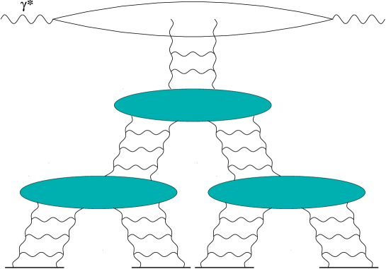
FIG. 1.: An example of the pomeron “fan” diagram, which were considered in deriving (2).

There have been several attempts to solve Eq. (2) analytically [11, 14]. Unfortunately it turned out to be very hard to construct an analytical solution describing simultaneously the behavior of $N_{0}({\bf x}_{01},{\bf b},Y)$ both outside and inside of the saturation region. Instead Eq. (2) was solved separately outside [$k>Q_{s}(Y)$] and inside [$k<Q_{s}(Y)$] the saturation region [11, 14], where approximately [11]

$$Q_{s}(Y)\sim\Lambda\,\alpha^{2}\,A^{1/3}\,\frac{\exp[(\alpha_{P}-1)Y]}{\sqrt{14\alpha N_{c}\zeta(3)Y}},$$ (4)

with $\alpha_{P}-1=\frac{4\alpha C_{F}}{\pi}\,\ln 2$. In [11, 14] it was concluded that for not very large energies, corresponding to rapidities of the order of $Y\sim 1/\alpha$ (or, equivalently, for $k>Q_{s}(Y)$ ), the solution of Eq. (2) behaves with energy like a single BFKL pomeron exchange, with multiple pomeron corrections setting in as energy increases and slowing down the growth of $N_{0}({\bf x}_{01},{\bf b},Y)$. For very high energies ($Y\geq\frac{1}{\alpha_{P}-1}\ln\frac{1}{\alpha^{2}}$ or $k<Q_{s}(Y)$) the solution of Eq. (2) saturates to a constant, namely $N_{0}({\bf x}_{01},{\bf b},Y)=1$, which corresponds to the blackness of the total cross section of the quark–antiquark pair on the nucleus [11, 14]. Thus, as one can see at least the qualitative features of $N_{0}({\bf x}_{\perp},{\bf b},Y)$ as a function of $Y$ and $x_{\perp}$ are known. For a better quantitative understanding of the behavior of $N_{0}({\bf x}_{\perp},{\bf b},Y)$ one should, probably, solve Eq. (2) numerically, which would be a very interesting and useful project to perform.

FIG. 2.: Single diffractive dissociation process considered in the paper. The interaction between the target and virtual photon is represented schematically by an exchange of a color singlet object.

In [7] the object of interest was the total inclusive DIS cross section, where no restrictions are imposed on the final state of the process. In this paper we are going to study the cross section of the single diffractive dissociation. The physical picture of the process we are going to consider is the following: in DIS the virtual photon interacts with the hadron or nucleus breaking up into hadrons and jets in the final state. At the same time the target hadron (nucleus) remains intact. The particles produced as a result of hadron’s breakup do not fill the whole rapidity interval, leaving a rapidity gap between the target and the “slowest” produced particle. The process is depicted in Fig. 2. In diffractive dissociation one imposes a restriction on the final state — the existence of a rapidity gap.

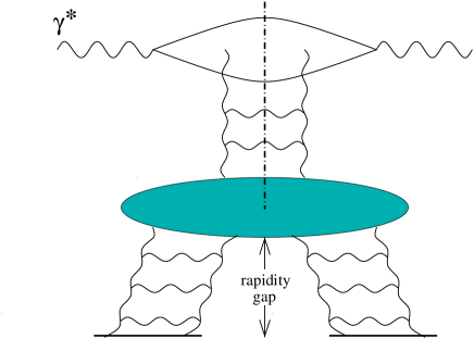
FIG. 3.: Traditional description of single diffractive dissociation. Dash-dotted line represents the final state.

Below we are going to employ the techniques of Mueller’s dipole model [1, 2, 3, 4], similarly to the way they were applied in [7], to construct a cross section of the single diffractive dissociation in DIS which would include the effects of multiple pomeron exchanges. Analogous to [7, 11] we will neglect the diagrams with pomeron loops, i.e. , the diagrams where a pomeron splits into two pomerons and then the two pomerons merge into one pomeron. As was argued in [7, 11, 12, 13] these diagrams are suppressed compared to the pomeron fan diagrams of Fig. 1 in DIS on a large nucleus by factors of $A^{1/3}$. Thus one can safely neglect them up to rapidities of the order of $Y{{}_{\displaystyle{>}}\atop\displaystyle{\sim}}\frac{1}{\alpha_{P}-1}\ln\frac{1}{\alpha^{2}A^{1/3}}$. For the case of DIS on a proton, strictly speaking there is no similar argument allowing one to neglect pomeron loop diagrams. Therefore, whereas the fan diagram evolution dominates in DIS on a nucleus, it could only be considered as a model for DIS on a hadron.

In the traditional description of the single diffractive dissociation one usually considers triple pomeron vertex [2, 15, 16, 17], where the pomeron above the vertex is cut, and the two pomerons below the vertex are on different sides of the cut, thus producing a rapidity gap, as shown in Fig. 3. That way the particles are produced by the cut pomeron in the rapidity interval adjacent to the virtual photon’s fragmentation region and no particles are produced with rapidities close to the final state of the target due to uncut pomerons. In this paper we want to enhance this picture by including multiple pomeron exchange diagrams. We would like to understand the behavior of the diffractive dissociation at very high energies, which may include some effects of saturation of hadronic or nuclear structure functions.

An example of a graph in the usual Feynman diagram language which we will consider below is given in Fig. 4. Dash-dotted line corresponds to the final state, i.e., to the cut. As one can see in Fig. 4 some of the pomerons are cut, some remain uncut. In the region of rapidity where pomerons are cut we have particles being produced. In the notation of Fig. 4 this corresponds to the interval in rapidity from $Y-Y_{0}$ to $Y$. In the region where the pomerons are uncut (rapidity interval from $0$ to $Y_{0}$) nothing is produced, which corresponds to a rapidity gap. That way Fig. 4 demonstrates a generalization of the traditional picture of Fig. (3), in which the cut pomeron splits into two pomerons, which later branch into two uncut pomerons each. Our goal in this paper is to resum all the diagrams where the cut pomeron can split into any number of cut pomerons via fan diagrams, and the cut pomerons in turn split into uncut pomerons, which can also branch into any number of uncut pomerons interacting with the target below.

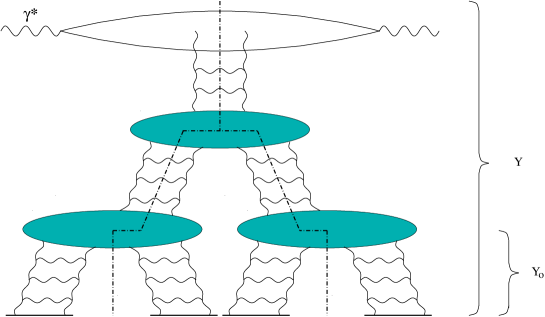
FIG. 4.: A diagram contributing to the diffractive dissociation with rapidity gap $Y_{0}$ as considered in the text.

In Sect. II we employ the dipole model formalism [1, 2, 3, 4] to write down an equation for the cross section of the single diffractive dissociation of a quark–antiquark pair on a hadron or nucleus with the rapidity gap bigger or equal to $Y_{0}$. The task is not very straightforward, since the dipole model provides us with the dipole wave function of the $q\overline{q}$ pair by the time it hits the target. In the rest frame of the target the typical time scale associated with the interaction is negligibly small compared to the typical lifetime of the QCD evolved wavefunction of the pair. Thus one could say that the interaction is instantaneous and happens at the time $t=0$ [18]. However, after the interaction, the $q\overline{q}$ state with many gluons in it can undergo several transformation until all the partons in it reach the mass shell at $t=\infty$. Dipole model does not provide us with any information about these final state interactions. Nevertheless one can gain control over the final state through the unitarity condition and cancelation of certain classes of final state interactions, as will be shown below. As a result we obtain a nonlinear evolution equation for the diffractive cross section, shown in formula (11).

We show how Eq. (11) can be re-derived by applying the AGK cutting rules to the pomeron fan diagrams in Sect. III. Since the cut or uncut pomerons precisely specify the final state in the traditional language, we, therefore, proved the consistency of our treatment of the final states in the dipole model.

Even though the exact analytical solution of that equation seems to be very complicated in Sect. IV we analyze the properties of the solution. As a toy model we consider a simplified version of the equation with the kernel independent of transverse coordinates. We show that the simplified equation’s solution exhibits a remarkable property at very high energies. We plot the cross section of diffractive dissociation events with rapidity gap $Y_{0}$ at fixed large center of mass energy as a function of the size of the rapidity gap $Y_{0}$. This is equivalent to plotting the cross section as a function of the invariant mass of the produced particles $M_{X}^{2}$, since, as could be easily seen from Fig. 2, $Y_{0}=Y-\ln M_{X}^{2}/Q^{2}$. At not very large $Y_{0}$ (large $M_{X}^{2}$) the cross section increases with the increase of rapidity gap, which agrees with the result of the traditional triple pomeron description of the diffractive dissociation of [2, 15]. However, as $Y_{0}$ gets very high comparable to the values of rapidity at saturation, which corresponds to a very small produced mass $M_{X}^{2}$, the cross section reaches a maximum and starts decreasing. That way if one would be able to measure the single diffractive cross section for a range of different invariant masses of the produced particles, one should be able to observe the maximum and turnover of the cross section for small masses if the energy is high enough for the saturation effects to become important. If the exact, probably numerical, solution of the equation confirms our conclusion, which was reached by approximate methods, then the single diffractive cross section is a new and independent observable which can be used to test whether the saturation region has been reached in DIS experiments.

The summary of our results is presented in Sect. V.

II Evolution equation for diffractive cross section

In this section we will write down an evolution equation resumming multiple pomeron exchanges for the cross section of single diffractive dissociation in DIS on a hadron or nucleus (see Figs. 2 and 4). As was mentioned in the introduction the task is complicated by the fact that the techniques of the dipole model [1, 2, 3, 4] which we are going to employ provide us with the state of the system at time $t=0$, without putting any restrictions on its subsequent time evolution until $t=\infty$. The dipole cascade is developed by the time of interaction and interacts with the nucleus at $t=0$ for any process. It is the subsequent time evolution of the cascade that determines whether the event is going to have a rapidity gap, which would correspond to some of the dipoles recombining, or not. This evolution is not included in the dipole model [1, 2, 3, 4]. However we will be able to constrain that time evolution after the interaction took place and to construct the diffractive cross section using the following two observations.

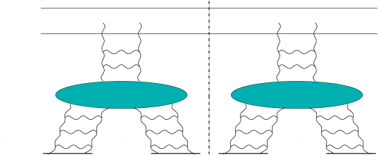
FIG. 5.: An example of elastic scattering of the quark–antiquark pair on the nucleus as pictured in the text.

The first observation is that if one knows the total cross section for a the scattering of some probe on a target one can easily construct the elastic scattering cross section out of it using unitarity constraints. Really, if the total cross section is [19, 20, 21]

$$\sigma_{tot}=2\int d^{2}b\,\,[1-S(b)]$$ (6)

with $S(b)$ the $S$–matrix of the scattering process at a fixed impact parameter $b$, then the elastic cross section is [19, 20, 21]

$$\sigma_{el}=\int d^{2}b\,\,[1-S(b)]^{2}.$$ (7)

Using Eqs. (6),(7) it was shown in [11, 19] that the elastic cross section for the scattering of the quark–antiquark pair generated by a virtual photon in DIS on a nucleus or hadron could be expressed in terms of the elastic amplitude $N_{0}({\bf x}_{01},{\bf b},Y)$, or, equivalently, in terms of the imaginary part of the forward scattering amplitude $N_{0}({\bf x}_{01},{\bf b},Y)d^{2}b$ (The forward amplitude is purely imaginary.). The result was [11, 19]

$$N^{el}({\bf x}_{01},{\bf b},Y)=N_{0}({\bf x}_{01},{\bf b},Y)^{2}$$ (8)

and is illustrated in Fig. 5. The cut in Fig. 5 corresponds to the final state, when the particles reached the mass shell and $t=\infty$. Thus in that picture we explicitly impose the constraint that not only the $q\overline{q}$ system developed a dipole cascade and the cascade in turn interacted with the target at $t=0$, but it also recombined back into a $q\overline{q}$ pair by the time the system reached the final state at $t=\infty$. Eq. (8) allows us to calculate the elastic cross section of the scattering of any (not necessarily original) dipole in the dipole cascade on the nucleus including multiple pomeron evolution.

The second observation which we have to make before starting to derive our equation is based on the work of Chen and Mueller [4] and concerns the so-called final state interactions. By that we mean the interactions such as branching or recombination of partons in the dipole cascade after $t=0$, i.e., after the interaction with the target. Chen and Mueller [4] succeeded in proving that certain classes of final state interactions cancel (see Fig. 6).

FIG. 6.: Classes of diagrams with final state interactions which cancel.

We denote a gluon by the double line in Fig. 6 corresponding to the large $N_{c}$ limit. In each diagram of Fig. 6 we assume that the summation over all possible connections of the gluon to the quark and antiquark lines is performed. In Fig. 6A we consider the situation when the gluon is emitted in a dipole after the interaction with the target at $t=0$, which is denoted by dotted line. The three different positions of the $t=\infty$ final state cut, denoted by dash-dotted line in Fig. 6A correspond to the cases when the emitted gluon is present in the final state and when the gluon recombines back in the amplitude or complex conjugate amplitude leaving the dipole intact by $t=\infty$. As was proved in [4] the sum of the three cuts of Fig. 6A is zero.

In Fig. 6B we consider the situation when the gluon was developed in the dipole wave function before the interaction with the target and is already there by the time $t=0$. Then it can either remain in the final state $t=\infty$ or it can recombine back, leaving only the original dipole in which it was produced in the final state. In Fig. 6B we explore the case when the gluon in the final state becomes a gluon emitted after $t=0$ in the complex conjugate amplitude (first diagram in Fig. 6B). Chen and Mueller [4] showed that this diagram is canceled by the second diagram in Fig. 6B.

Diagrams of Fig. 6 demonstrate that the contribution of gluons produced or absorbed after $t=0$ cancels out in calculation of inclusive quantities such as the total cross section. We can now conclude that the total inclusive DIS cross section can be calculated using just $t=0$ formalism, as was done in [7]. Really, as one can see from Fig. 6 all the final state interactions cancel, effectively leaving the $t=0$ state unchanged by $t=\infty$. This conclusion is intuitively easy to understand: one just needs to have some interaction of the projectile with the target to include the diagram in the total cross section, independent of what happened after that interaction.

Now we are ready to write down our equation for diffractive cross section. Let us start by defining the object for which the equation will be written. We denote by $N^{D}({\bf x}_{\perp},{\bf b},Y,Y_{0})$ the cross section of single diffractive dissociation of a dipole of transverse size ${\bf x}_{\perp}$, rapidity $Y$ and impact parameter ${\bf b}$ on a target hadron or nucleus. The process has a rapidity gap covering a rapidity interval adjacent to the target (see Fig. 2,4 ) which could be greater or equal than $Y_{0}$. The corresponding diffractive structure function, similarly to Eq. (1), is

$$F_{2}^{SD}(x,Q^{2},Y_{0})=\frac{Q^{2}}{4\pi^{2}\alpha_{EM}}\int\frac{d^{2}{\bf x}_{01}dz}{4\pi}\,\Phi({\bf x}_{01},z)\ d^{2}b\ N^{D}({\bf x}_{01},{\bf b},Y,Y_{0}).$$ (9)

If one wishes to obtain a cross section of diffractive dissociation of the dipole with a fixed rapidity gap $Y_{0}$ one has to differentiate $N^{D}$ with respect to $Y_{0}$, as will be discussed later. When $Y=Y_{0}$ the rapidity gap fills out the whole rapidity interval, turning the process of dipole’s dissociation into an elastic scattering. Taking the answer for elastic process from Eq. (8) we obtain an initial condition for the evolution of $N^{D}$

$$N^{D}({\bf x}_{\perp},{\bf b},Y=Y_{0},Y_{0})=N_{0}^{2}({\bf x}_{\perp},{\bf b},Y_{0}).$$ (10)

Note that Eq. (10) insures that after the interaction with the target at $t=0$ the system of developed dipoles only recombines back into the original dipole by $t=\infty$. All other possible final state fluctuations have been excluded because we explicitly put $N_{0}^{2}({\bf x}_{\perp},{\bf b},Y_{0})$ as the amplitude of the elastic process.

To construct $N^{D}$ one has to require that nothing is produced in the $t=\infty$ final state in the rapidity interval from $0$ to $Y_{0}$, where the target hadron or nucleus is situated at rapidity $0$. This does not restrain the rapidity gaps from being greater than $Y_{0}$. That way $N^{D}$ would include all events with rapidity gap greater or equal to $Y_{0}$. The condition of the rapidity gap up to $Y_{0}$ is satisfied by Eq. (10).

As was mentioned above our physical picture of the diffractive dissociation event is the following: before hitting the target the virtual photon develops a dipole cascade, which at the time $t=0$ interacts with the target. After that some partons in the cascade may recombine, producing rapidity gaps, some may not. By imposing the recombination condition in Eq. (10) we made sure that the dipoles with rapidities $y<Y_{0}$ will recombine by $t=\infty$, producing a rapidity gap. The dipoles with $y>Y_{0}$ are free to either recombine into the dipoles off which they were produced or to remain unchanged till $t=\infty$. As long as $y>Y_{0}$ there are no restrictions on the final state like rapidity gaps. Therefore the dipoles are free to recombine after $t=0$. However, for that situation the cancelation rules proven by Chen and Mueller [4] apply. The graphs when the dipoles recombine to either increase the size of the rapidity gap $Y_{0}$ or to produce extra rapidity gaps at $y>Y_{0}$ are included, but as one can see from Fig. 6B they cancel. For the asymmetric case when the dipole in consideration interacts with the target in the amplitude and then recombines back into the dipole off which it was produced which has no interaction with the target in the complex conjugate amplitude we employ a different cancelation mechanism: the contributions when the dipole recombines in the complex conjugate amplitude at the times $t>0$ and $t<0$ cancel each other, leaving us with the diagram of similar to the second graph of Fig. 6B, which could be incorporated in the elastic interaction of the original dipole with the target $N_{0}({\bf x}_{\perp},{\bf b},y)$. That way the asymmetric graphs may include the dipoles of any rapidities $y>Y_{0}$ interacting elastically with the target via Eq. (10). For the “symmetric” case when the dipole at $y>Y_{0}$ interacts elastically with the target in the amplitude and then recombines into the original dipole which interacts with the target elastically in the complex conjugate amplitude we applied the cancelation of Fig. 6B. Thus the symmetric case reduces to the situation when the same dipole interacts elastically in the amplitude and complex conjugate amplitude at $y=Y_{0}$ and is put only in the initial condition of our equation given by $N_{0}^{2}({\bf x}_{\perp},{\bf b},Y_{0})$.

Dipole splitting is a little more complicated. The softest dipoles in the cascade interact the way it is described in Eq. (10), which fixes the final state for them. Now let us consider a dipole which is not one of these soft dipoles and, therefore, does not interact with the target. The dipole can split into two dipoles either before or after $t=0$. This event is allowed only when the produced real gluon has the rapidity greater or equal than $Y_{0}$, so that it would not destroy the rapidity gap. In that case the real gluon emitted before $t=0$ is canceled by a virtual correction in the same dipole before $t=0$. The real gluon emitted after $t=0$ is canceled by the virtual term after $t=0$, similarly to Fig. 6A. Finally, this non-interacting dipole can develop a virtual corrections with the gluon being softer than $Y_{0}$, i.e. having smaller rapidity than the rapidity of the gap. These gluons could not be canceled by the real contributions, since those are excluded by the condition of the gap’s existence. However, since the virtual corrections could happen either before or after $t=0$, these two combinations come with different signs. The absolute values of both $t>0$ and $t<0$ contributions in that case are the same and, therefore, they cancel each other. Thus we have shown that the final state dipole splitting is canceled together with the virtual corrections in the non-interacting dipoles.

The above discussion is summarized in Fig. 7. The change of the cross section of diffractive dissociation $N^{D}$ in one step of the rapidity evolution could be generated by several terms on the right hand side of the equation in Fig. 7. The first terms corresponds to the usual single BFKL pomeron evolution, while the rest of the terms correspond to the triple pomeron vertex, similarly to the equation written in [1, 7]. Effectively Fig. 7 states that in one step of evolution the color dipole splits into two dipoles. The subsequent evolution can happen in one of the dipoles, which corresponds to the first term on the right hand side of Fig. 7. It could also happen that we continue the evolution leading to the cross section of diffractive dissociation in both dipoles (the second terms in Fig. 7). The third and forth terms correspond to the asymmetric cases. As was discussed above in the asymmetric case the dipole can interact elastically with the target in the amplitude but not in the complex conjugate amplitude and vice versa at any rapidity $Y>Y_{0}$. Thus we include the cases when only one of the produced dipoles interacts asymmetrically with the target (the third term in Fig. 7) and when both of them do so (the fourth term in Fig. 7). The coefficients in front of different terms come from combinatorics. Note that they match the coefficients of the Abramovskii, Gribov, Kancheli (AGK) [16] cutting rules for two pomeron contributions.

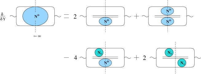
FIG. 7.: The equation for the cross section of diffractive dissociation.

Recalling the initial condition of Eq. (10) we can turn the picture of Fig. 7 into a formula. For that we also have to include the virtual corrections similarly to the way they were included in [1]. The resulting equation is

$$N^{D}({\bf x}_{01},{\bf b},Y,Y_{0})=N_{0}^{2}({\bf x}_{01},{\bf b},Y_{0})\,e^{-\frac{4\alpha C_{F}}{\pi}\ln\left(\frac{x_{01}}{\rho}\right)(Y-Y_{0})}+\frac{\alpha C_{F}}{\pi^{2}}\int_{Y_{0}}^{Y}dy\,e^{-\frac{4\alpha C_{F}}{\pi}\ln\left(\frac{x_{01}}{\rho}\right)(Y-y)}$$

$$\times\int_{\rho}d^{2}x_{2}\frac{x_{01}^{2}}{x_{02}^{2}x_{12}^{2}}\,[2\,N^{D}({\bf x}_{02},{\bf b}+\frac{1}{2}{\bf x}_{12},y,Y_{0})+N^{D}({\bf x}_{02},{\bf b}+\frac{1}{2}{\bf x}_{12},y,Y_{0})\,N^{D}({\bf x}_{12},{\bf b}+\frac{1}{2}{\bf x}_{02},y,Y_{0})$$

$$-4\,N^{D}({\bf x}_{02},{\bf b}+\frac{1}{2}{\bf x}_{12},y,Y_{0})\,N_{0}({\bf x}_{12},{\bf b}+\frac{1}{2}{\bf x}_{02},y)+2\,N_{0}({\bf x}_{02},{\bf b}+\frac{1}{2}{\bf x}_{12},y)\,N_{0}({\bf x}_{12},{\bf b}+\frac{1}{2}{\bf x}_{02},y)].$$ (11)

The shifts in the impact parameter dependence of the functions on the right hand side of Eq. (11) have occurred because the centers of mass of the produced dipoles are located at different impact parameters than the center of mass of the initial dipole.

Eq. (11) describes the small-$x$ evolution of the cross section of the single diffractive dissociation for DIS $N^{D}$ and is the central result of this paper.

III Rederiving evolution equation with AGK cutting rules

Eq. (11) can also be derived using the technique employing the AGK cutting rules [16]. In this section we will not employ the dipole model. Instead we will consider pomeron fan diagrams in the usual perturbation theory, imposing a restriction that there are only triple pomeron vertices in the theory. This assumption is true only in the large $N_{c}$ limit, as was shown in the dipole model.

AGK cutting rules [16] apply to the BFKL pomerons in QCD (see [22] for a detailed discussion). For the BFKL pomeron one can write

$$2\,\mbox{Im}\,a^{BFKL}_{el}=G_{in}^{BFKL},$$ (12)

where $a^{BFKL}_{el}$ is the one BFKL pomeron contribution to the forward scattering amplitude and $G_{in}^{BFKL}$ is the total inelastic cross section. In writing Eq. (12) we have neglected the elastic contribution to the cross section, which is a justified assumption for the BFKL pomeron exchange [22]. Eq. (12) tells us that the inelastic cross section in one pomeron exchange approximation is twice the forward amplitude of the process, since the latter is purely imaginary.

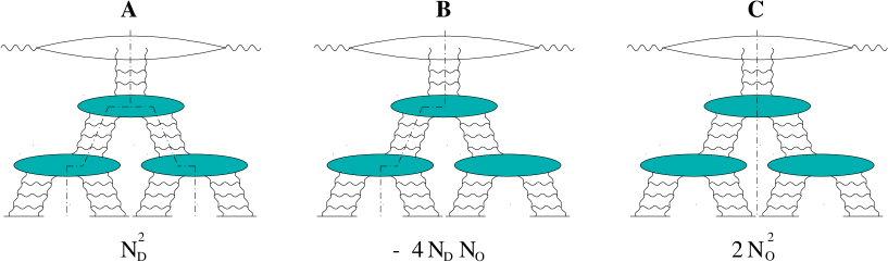
FIG. 8.: Different pomeron cuts contributing to the cross section of diffractive dissociation which lead to different terms on the right hand side in Eq. (11).

Different cuts of pomeron fan diagrams corresponding to the terms on the right hand side of Eq. (11) are displayed in Fig. 8. The first (linear) term on the right hand side of Eq. (11) corresponds to just usual linear BFKL evolution with the factor of $2$ arising from Eq. (12) and is not shown in Fig. 8. The non-linear evolution corresponds to a pomeron splitting into two via the triple pomeron vertices. Let us now concentrate on the first (topmost) triple pomeron vertex in the diagrams of Fig. 8. This is where one step of non-linear evolution takes place in our picture. The graph of Fig. 8A corresponds to the case when a cut pomeron splits into two cut pomerons, which later on produce rapidity gaps. That is the cross section of diffractive dissociation $N_{D}$ splits into two similar cross sections. Therefore this term gives rise to $N_{D}^{2}$ term in Eq. (11). The factor in front of this term results from multiplying $2$ from the cut pomeron on top of the vertex by the symmetry factor of $1/2$. The diagram of Fig. 8B corresponds to a cut pomeron splitting into another cut pomeron, which then develops a rapidity gap ($N_{D}$), and an uncut pomeron, corresponding to the forward scattering amplitude $N_{0}$. Since there are two of such diagrams, multiplying the factor of $2$ of the cut pomeron by $2$ and putting a minus sign since one of the resulting pomerons is completely on one side of the cut we will get $-4N_{D}N_{0}$, which is the contribution of that diagram in Eq. (11). Finally the graph of Fig. 8C corresponds to the case when both of the pomerons below the vertex are uncut. Each uncut pomeron gives a factor of $N_{0}$. The factor of $2$ arises from the cut pomeron above [Eq. (12)].

Therefore we were able to reproduce all the terms on the right hand side of Eq. (11) from the usual pomeron fan diagrams using the AGK cutting rules. We note that a similar result was obtained in the framework of reggeon theory in [23]. The cut (or uncut) pomeron specifies $t=\infty$ final state very precisely: if the pomeron is cut it insures that there will be particles produced in the final state. Uncut pomeron insures that nothing is produced in the $t=\infty$ final state. Thus in this section we have demonstrated the consistency of our analysis of the evolution of the dipole state after the interaction with the target which was employed in the previous section.

IV Properties of the solution of the evolution equation

Eq. (11) can be rewritten in the differential form. Similar to what was done in [7] we differentiate both sides of Eq. (11) with respect to $Y$ and once again make use of Eq. (11) to obtain

$$\frac{\partial N^{D}({\bf x}_{01},{\bf b},Y,Y_{0})}{\partial Y}=\frac{2\alpha C_{F}}{\pi^{2}}\,\int_{\rho}d^{2}x_{2}\left[\frac{x^{2}_{01}}{x^{2}_{02}x^{2}_{12}}-2\pi\delta^{2}({\bf x}_{01}-{\bf x}_{02})\ln\left(\frac{x_{01}}{\rho}\right)\right]N^{D}({\bf x}_{02},{\bf b}+\frac{1}{2}{\bf x}_{12},Y,Y_{0})$$

$$+\frac{\alpha C_{F}}{\pi^{2}}\,\int d^{2}x_{2}\,\frac{x^{2}_{01}}{x^{2}_{02}x^{2}_{12}}\,[N^{D}({\bf x}_{02},{\bf b}+\frac{1}{2}{\bf x}_{12},Y,Y_{0})\,N^{D}({\bf x}_{12},{\bf b}+\frac{1}{2}{\bf x}_{02},Y,Y_{0})$$

$$-4\,N^{D}({\bf x}_{02},{\bf b}+\frac{1}{2}{\bf x}_{12},Y,Y_{0})\,N_{0}({\bf x}_{12},{\bf b}+\frac{1}{2}{\bf x}_{02},Y)+2\,N_{0}({\bf x}_{02},{\bf b}+\frac{1}{2}{\bf x}_{12},Y)\,N_{0}({\bf x}_{12},{\bf b}+\frac{1}{2}{\bf x}_{02},Y)],$$ (13)

with Eq. (10) being the initial condition for the differential equation (13).

Let us define the following object

$${\cal F}({\bf x}_{01},{\bf b},Y,Y_{0})=2\,N_{0}({\bf x}_{01},{\bf b},Y)-N^{D}({\bf x}_{01},{\bf b},Y,Y_{0})\,\theta(Y-Y_{0}),$$ (14)

which has the meaning of the cross section of the events with rapidity gaps less than $Y_{0}$. The theta-function that multiplies $N^{D}$ in Eq. (14) insures the trivial fact that the rapidity gap can not be larger than the total rapidity interval. One can see that Eq. (13) can be rewritten for $Y_{0}\leq Y$ in terms of ${\cal F}$ as

$$\frac{\partial{\cal F}({\bf x}_{01},{\bf b},Y,Y_{0})}{\partial Y}=\frac{2\alpha C_{F}}{\pi^{2}}\,\int_{\rho}d^{2}x_{2}\left[\frac{x^{2}_{01}}{x^{2}_{02}x^{2}_{12}}-2\pi\delta^{2}({\bf x}_{01}-{\bf x}_{02})\ln\left(\frac{x_{01}}{\rho}\right)\right]{\cal F}({\bf x}_{02},{\bf b}+\frac{1}{2}{\bf x}_{12},Y,Y_{0})$$

$$-\frac{\alpha C_{F}}{\pi^{2}}\,\int d^{2}x_{2}\,\frac{x^{2}_{01}}{x^{2}_{02}x^{2}_{12}}\,{\cal F}({\bf x}_{02},{\bf b}+\frac{1}{2}{\bf x}_{12},Y,Y_{0})\,{\cal F}({\bf x}_{12},{\bf b}+\frac{1}{2}{\bf x}_{02},Y,Y_{0}),$$ (15)

with the initial condition

$${\cal F}({\bf x}_{01},{\bf b},Y=Y_{0},Y_{0})=2\,N_{0}({\bf x}_{01},{\bf b},Y_{0})-N_{0}^{2}({\bf x}_{01},{\bf b},Y_{0}).$$ (16)

If one differentiates Eq. (2) with respect to $Y$ one would obtain the same differential equation as Eq. (15) for $N_{0}$

$$\frac{\partial N_{0}({\bf x}_{01},{\bf b},Y)}{\partial Y}=\frac{2\alpha C_{F}}{\pi^{2}}\,\int_{\rho}d^{2}x_{2}\left[\frac{x^{2}_{01}}{x^{2}_{02}x^{2}_{12}}-2\pi\delta^{2}({\bf x}_{01}-{\bf x}_{02})\ln\left(\frac{x_{01}}{\rho}\right)\right]N_{0}({\bf x}_{02},{\bf b}+\frac{1}{2}{\bf x}_{12},Y)$$

$$-\frac{\alpha C_{F}}{\pi^{2}}\,\int d^{2}x_{2}\,\frac{x^{2}_{01}}{x^{2}_{02}x^{2}_{12}}\,N_{0}({\bf x}_{02},{\bf b}+\frac{1}{2}{\bf x}_{12},Y)\,N_{0}({\bf x}_{12},{\bf b}+\frac{1}{2}{\bf x}_{02},Y).$$ (17)

The initial condition for Eq. (17) is different from that for Eq. (15)

$$N_{0}({\bf x}_{01},{\bf b},Y=0)=\gamma({\bf x}_{01},{\bf b})$$ (18)

with $\gamma({\bf x}_{01},{\bf b})$ given by Eq. (3). From Eq. (14) one can see now that in order to find $N^{D}({\bf x}_{01},{\bf b},Y,Y_{0})$ one has to solve the same equation [(15) or (17)] for two different initial conditions given by formulae (16) and (18), which would yield us with the results for $N_{0}$ and ${\cal F}$. Then $N^{D}$ could be found using Eq. (14).

As was mentioned above the exact analytical solution of Eq. (15), or, equivalently, (17) has not been found [11, 14]. Nevertheless the qualitative behavior of the solution of this equation is understood very well, with some quantitative estimates performed [11, 14]. It turned out that the solution of this equation can be qualitatively well approximated by the solution of the equation with suppressed transverse coordinate dependence

$$\frac{\partial N_{0}(Y)}{\partial Y}=(\alpha_{P}-1)\,N_{0}(Y)-(\alpha_{P}-1)\,N_{0}(Y)^{2}.$$ (19)

Eq. (19) is a toy model of the full Eq. (17), with all the transverse coordinate integrations suppressed and the dipole BFKL kernel substituted by its eigenvalue at the BFKL saddle point. The fact that the coefficients in front of the linear and quadratic terms in Eq. (19) are identical could, for instance, be understood in the double logarithmic limit ($x_{02},x_{12}\ll x_{01}$), in which the kernel in front of the quadratic term in Eq. (17) produces an extra factor of two and becomes equal to the kernel in front of the linear term [11, 14]. However it is a more general property of the solution of Eq. (17), which is valid not only in the double logarithmic limit.

In this paper we will try to understand the qualitative behavior of the solution of Eq. (11) using the toy model of Eq. (19). An exact, probably numerical, solution of Eq. (17) would give more precise results for $N^{D}$. However, we believe that the qualitative features provided by the toy model of Eq. (19) will be preserved in the exact solution.

Let us suppose that $N_{0}(Y)$ is a solution of Eq. (17), or, in our toy model, of Eq. (19). Then ${\cal F}(Y,Y_{0})$ will be a solution of the same equation with different initial condition set at a different value of rapidity (see Eq. (16)). Thus, if we neglect the transverse coordinate dependence, the solution for ${\cal F}(Y,Y_{0})$ could be obtained from the solution for $N_{0}(Y)$ just by a shift in rapidity. Define the shift variable $\Delta Y$ by

$$N_{0}(Y_{0}+\Delta Y)=2\,N_{0}(Y_{0})-N_{0}(Y_{0})^{2}$$ (20)

so that

$${\cal F}(Y,Y_{0})=N_{0}(Y+\Delta Y).$$ (21)

Now one can see that since $N_{0}(Y)$ satisfies the differential equation (17) (or Eq. (19) in our toy model), then ${\cal F}(Y,Y_{0})$ given by Eq. (21) satisfies the same equation (19) with the initial condition of Eq. (16). Of course this is true only when one neglects the transverse coordinate dependence of $N_{0}$ and ${\cal F}$, but could also be a reasonable approximation for the case of weak transverse coordinate dependence.

Solving Eq. (19) with the initial condition $N_{0}(Y=0)=\gamma$ we obtain

$$N_{0}(Y)=\frac{\gamma e^{(\alpha_{P}-1)Y}}{1+\gamma(e^{(\alpha_{P}-1)Y}-1)},$$ (22)

which employing Eq. (20) yields us with the following expression for $\Delta Y$

$$\Delta Y=\frac{1}{\alpha_{P}-1}\ln\left(2+\frac{\gamma}{1-\gamma}e^{(\alpha_{P}-1)Y_{0}}\right).$$ (23)

Eq. (21) allows us to write down a toy model expression for ${\cal F}$

$${\cal F}(Y,Y_{0})=\frac{\gamma e^{(\alpha_{P}-1)Y}\left(2+\frac{\gamma}{1-\gamma}e^{(\alpha_{P}-1)Y_{0}}\right)}{1-\gamma+\gamma e^{(\alpha_{P}-1)Y}\left(2+\frac{\gamma}{1-\gamma}e^{(\alpha_{P}-1)Y_{0}}\right)}.$$ (24)

Now we can explore the qualitative behavior of our result. First we note that for not very large rapidities, $Y\sim 1/\alpha$, we can put denominators in Eqs. (22) and (24) to be equal to $1$, which through Eq. (14) provides us with

$$-\frac{\partial N^{D}(Y,Y_{0})}{\partial Y_{0}}\approx(\alpha_{P}-1)\gamma^{2}e^{(\alpha_{P}-1)(Y+Y_{0})}+\delta(Y-Y_{0})N_{0}^{2}(Y_{0}).$$ (25)

The first term on the right hand side of Eq. (25) is the usual result of the lowest order approach employing only one triple pomeron vertex [2, 15] (see Fig. 3). The second (delta-function) term in Eq. (25) corresponds to the contribution of the elastic cross section when the rapidity gap fills the whole rapidity interval.

Remember that $N^{D}(Y,Y_{0})$ is the cross section of having a rapidity gap greater or equal to $Y_{0}$. If one wants to obtain the cross section for a fixed size of the rapidity gap one has to differentiate $N^{D}$ with respect to $Y_{0}$ and take a negative of the result, since $N^{D}$ is obviously a decreasing function of $Y_{0}$. This is what was done in arriving at Eq. (25). That way we have verified that the toy model solution of our equation (11) maps onto the old and well established triple pomeron vertex result [15].

At the lowest order $\gamma\sim\alpha^{2}A^{1/3}$. Thus the first term on the right hand side of Eq. (25), which is usually calculated in the perturbative approaches [15], is of the order of $\alpha^{5}\ll 1$. We note that using the nonlinear evolution equation (2) we were able to obtain control over the kinematic regions where the coupling is still small but the cross sections can become very large, with $N_{0}\sim 1$. Thus the traditional perturbative calculation of Eq. (25) appears like a small perturbation compared to our large cross section result of Eq. (22), which was still obtained in the small coupling constant limit.

At very high energies, when $Y\rightarrow\infty$, one can see from Eqs. (22),(24) and (14) that

$$N^{D}(Y,Y_{0})\rightarrow 1,\,\,\,Y\rightarrow\infty.$$ (26)

This result is easy to understand. As we know from quantum mechanics at very high energies, when the total cross section is black, only the elastic and inelastic contributions to the cross section survive to give half of the total cross section each. The total cross section becomes $\sigma_{tot}=2\pi R^{2}$, whereas totally inelastic and elastic cross sections will be $\sigma_{inel}=\sigma_{el}=\pi R^{2}$. All the intermediate contributions with finite size rapidity gaps covering fraction of the total rapidity interval go to zero. Since $N^{D}(Y,Y_{0})$ is the cross section of having rapidity gap greater or equal than $Y_{0}$ for any finite non-zero $Y_{0}$ it includes the contribution of the elastic cross section, which corresponds to the case when the rapidity gap covers the whole rapidity interval. At the same time $N^{D}(Y,Y_{0})$ does not include the totally inelastic contribution, when there is no rapidity gap at all. Thus as at $Y\rightarrow\infty$ only the elastic piece in $N^{D}$ survives to give half of the total cross section, which corresponds to $N^{D}\rightarrow 1$ in our notation, where everything has to be multiplied by $\pi R^{2}$.

Let us define the cross section of single diffractive dissociation with the fixed rapidity gap $Y_{0}$, which, for $Y_{0}\leq Y$, in the light of the above discussion is

$$R({\bf x}_{01},{\bf b},Y,Y_{0})=-\frac{\partial N^{D}({\bf x}_{01},{\bf b},Y,Y_{0})}{\partial Y_{0}}=\frac{\partial{\cal F}({\bf x}_{01},{\bf b},Y,Y_{0})}{\partial Y_{0}}+\delta(Y-Y_{0})N_{0}^{2}({\bf x}_{01},{\bf b},Y_{0}).$$ (27)

In the toy model we have

$$R(Y,Y_{0})=\frac{\gamma^{2}(1-\gamma)^{2}(\alpha_{P}-1)e^{(\alpha_{P}-1)(Y+Y_{0})}}{\left[1+2\gamma\left(e^{(\alpha_{P}-1)Y}-1\right)+\gamma^{2}\left(1-2e^{(\alpha_{P}-1)Y}+e^{(\alpha_{P}-1)(Y+Y_{0})}\right)\right]^{2}}+\delta(Y-Y_{0})N_{0}^{2}(Y_{0}).$$ (28)

Now one can see that the triple pomeron vertex result of Eq. (25) could be recovered from the first term of Eq. (28) by putting the denominator to be $1$ and neglecting $\gamma$ with respect to $1$ in the numerator. Also the quantum mechanical result discussed above is illustrated explicitly: for any finite $Y_{0}$ the cross section of a fixed size gap $R(Y,Y_{0})$ goes to zero as $Y\rightarrow\infty$, as could be derived from Eq. (28).

Finally, let us plot the cross section of diffractive dissociation $R(Y,Y_{0})$ of Eq. (28) as a function of the size of rapidity gap $Y_{0}$ for a fixed center of mass rapidity $Y$ excluding the elastic cross section (delta-function) contribution. This is equivalent to plotting the cross section as a function of the invariant mass of the particles produced in the virtual photon’s decay, since $Y_{0}=Y-\ln M_{X}^{2}/Q^{2}$ (see Fig. 2). The plot is shown in Fig. 9. There we put $\alpha_{P}-1=.5$, $\gamma=.03$, $Y=10$ and we divided $Y_{0}$ by $Y$ on the horizontal axis.

Fig. 9 demonstrates that the cross section increases with the size of the rapidity gap over most of the rapidity interval. This is what one would expect from the lowest order formula (25). Also that implies that it is more advantageous to produce particles with smaller invariant mass $M_{X}^{2}$. However at some very large size of the rapidity gap the cross section $R(Y,Y_{0})$ reaches a maximum and starts decreasing. The maximum of $R(Y,Y_{0})$ in Eq. (28) is reached at the size of the rapidity gap

$$Y_{0}^{max}=\frac{1}{\alpha_{P}-1}\,\ln\left(\frac{2(1-\gamma)}{\gamma}+\frac{(1-\gamma)^{2}}{\gamma^{2}}e^{-(\alpha_{P}-1)Y}\right).$$ (29)

From Eq. (29) we can immediately conclude that if the target nucleus is very large so that each of the dipoles undergoes many rescatterings making $\gamma\approx 1$ the maximum will be pushed all the way into the region of negative $Y_{0}$, making the cross section of Fig. 9 just a decreasing function of $Y_{0}$ for all rapidities of interest. Thus, if the effects of multiple rescatterings of individual dipoles become important then the qualitative behavior of the cross section of diffractive dissociation will change completely. The effect of multiple rescattering is to push the maximum of Eq. (29) towards the smaller values of rapidity, which are easier to reach experimentally.

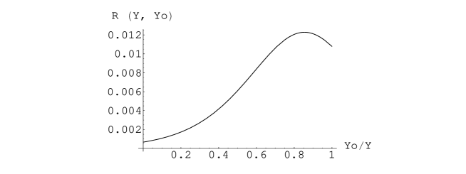
FIG. 9.: The cross section of diffractive dissociation in units of $\pi R^{2}$ at fixed $Y$ as a function of $Y_{0}$, which is scaled by $Y$. The elastic contribution is not included.

If the multiple dipole rescatterings are not very important we can just use the lowest order (one rescattering) $\gamma\sim\alpha^{2}A^{1/3}\ll 1$ and consider two limits. At not very large values of rapidity, $Y\sim 1/\alpha$, when the single BFKL pomeron exchange is most important the maximum can never be reached since

$$Y_{0}^{max}\sim\frac{1}{\alpha_{P}-1}\,\ln\frac{1}{\alpha^{2}A^{1/3}}\gg\frac{1}{\alpha_{P}-1}.$$ (30)

As energy increases and becomes of the order of saturation energy, corresponding to rapidities of the order of

$$Y_{sat}\sim\frac{1}{\alpha_{P}-1}\,\ln\frac{1}{\alpha^{2}A^{1/3}}$$ (31)

the maximum will be reached and the effect should be observed.

We can conclude that experimental observation of the maximum of the cross section of diffractive dissociation at certain size of the rapidity gap would signify the presence of multiple rescattering effects either in multiple pomeron exchanges, which are encoded in the branching of the dipole wave function, or in multiple interactions of each of the dipoles with the target, which were enclosed in the initial condition (3). Therefore it would be an independent test of whether the evolution equations describing the hadronic or nuclear structure functions should be still used at the linear order or non-linear effects like in Eq. (2) should be taken into account. The qualitative conclusion will also be independent of the non-perturbative initial conditions of the evolution equations. Here we have to warn the reader that our results in this section are based on the toy model and a more elaborate numerical analysis of Eq. (2) is needed to achieve the required level of rigor in these conclusions. Also Eq. (2) resums fan diagrams, leaving out the pomeron loop contributions. Even though pomeron loops are always suppressed by powers of $A$ compared to fan diagrams, they will become important at the rapidities of the order of $Y\sim\frac{1}{\alpha_{P}-1}\,\ln\frac{1}{\alpha^{2}}$. This is still above the saturation energy of Eq. (31) and does not affect much the kinematic region considered above. Nevertheless for real life nuclei the suppression of pomeron loop diagrams is not that large and they may play an important role already at the rapidities of interest.

V Conclusions

In this paper we have derived the small-$x$ evolution equation for the cross section of single diffractive dissociation (11). It resums multiple BFKL pomeron exchange diagrams contributing to the diffractive cross section. The equation is not derived in the framework of any model of multiple exchanges: it was directly derived from QCD. We made use of the fact that in DIS with large $Q^{2}$ the strong coupling constant is small. We also employed the leading logarithmic approximation resumming logarithms of Bjorken $x$ [5, 6]. Finally we employed the large $N_{c}$ limit of QCD at high energies — Mueller’s dipole model [1, 2, 3, 4].

The obtained equation (11) is nonlinear and most likely can not be solved analytically. We solved a simplified model of the equation (Eqs. (22) and (24)), in which the transverse coordinate dependence was suppressed. We believe that this approximation preserves the qualitative features of the solution. In this toy model we observed an interesting phenomenon: the diffractive cross section has a maximum as a function of the rapidity gap $Y_{0}$ (Fig. 9). This effect can not be obtained from the usual single triple pomeron vertex approach of [15, 2] and if experimentally observed would signify the importance of non-linear effects in QCD evolution of structure functions. The effect should be seen in the physically measurable quantity — DIS diffractive cross section and it would be an independent evidence of the onset of saturation.

REFERENCES

- [1] A.H. Mueller, Nucl. Phys. B415, 373 (1994).
- [2] A.H. Mueller and B. Patel, Nucl. Phys. B425, 471 (1994).
- [3] A.H. Mueller, Nucl. Phys. B437, 107 (1995).
- [4] Z. Chen, A.H. Mueller, Nucl. Phys. B451, 579 (1995).
- [5] E.A. Kuraev, L.N. Lipatov and V.S. Fadin, Sov. Phys. JETP 45, 199 (1977).
- [6] Ya.Ya. Balitsky and L.N. Lipatov, Sov. J. Nucl. Phys. 28, 22 (1978).
- [7] Yu. V. Kovchegov, Phys. Rev. D 60, 034008 (1999).
- [8] L.V. Gribov, E.M. Levin, and M.G. Ryskin, Nucl. Phys. B188, 555 (1981); Phys. Reports 100, 1 (1983).
- [9] I. I. Balitsky, hep-ph/9706411; Nucl. Phys. B463, 99 (1996).
- [10] A.H. Mueller, Nucl. Phys. B335, 115 (1990).
- [11] Yu. V. Kovchegov, hep-ph/9905214.
- [12] A. Schwimmer, Nucl. Phys. B 94, 445 (1975).
- [13] A.L. Ayala, M.B. Gay Ducati, and E.M. Levin, Nucl. Phys. B493, 305 (1997); Nucl. Phys. B551, 355 (1998).
- [14] E. Levin and K. Tuchin, hep-ph/9908317.
- [15] A. H. Mueller, Phys. Rev. D2, 2963 (1970); Phys. Rev. D2, 150 (1971).
- [16] V. A. Abramovskii, V. N Gribov, and O. V. Kancheli, Sov. J. Nucl. Phys. , Vol. 8, No. 3, (1974).
- [17] M Wusthoff and A. D. Martin, hep-ph/9909362; E. Levin and M. Wusthoff, Phys. Rev. D 50, 4306 (1994).
- [18] Yu. V. Kovchegov, A.H. Mueller, Nucl. Phys. B 529, 451 (1998).
- [19] Yu. V. Kovchegov, L. McLerran, Phys. Rev. D 60, 054025 (1999).
- [20] A. H. Mueller, Eur. Phys. J. A1, 19(1998).
- [21] M. Froissart, Phys. Rev. 123, 1053 (1961); E. Levin, hep-ph/9808486 and references therein.
- [22] J. Bartels, M.G. Ryskin, Z. Phys. C76,241 (1997) and references therein.
- [23] S. Bondarenko, E. Gotsman, E. Levin, and U. Maor, in preparation.