Features in the primordial power spectrum of double D-term inflation

Abstract

Recently, there has been some interest for building supersymmetric models of double inflation. These models, realistic from a particle physics point of view, predict a broken-scale-invariant power spectrum of primordial cosmological perturbations, that may explain eventual non-trivial features in the present matter power spectrum. In previous works, the primordial spectrum was calculated using analytic slow-roll approximations. However, these models involve a fast second-order phase transition during inflation, with a stage of spinodal instability, and an interruption of slow-roll. For our previous model of double D-term inflation, we simulate numerically the evolution of quantum fluctuations, taking into account the spinodal modes, and we show that the semi-classical approximation can be employed even during the transition, due to the presence of a second inflaton field. The primordial power spectrum possesses a rich structure, and possibly, a non-Gaussian spike on observable scales.
PACS : 98.80.Cq; 04.62.+v; 05.70.Fh
Keywords : Early universe; Inflation; Primordial fluctuations; Phase transitions

1 Introduction

The standard inflationary prediction [1] concerning the primordial power spectrum of scalar metric perturbations (denoted $\Phi$ in the longitudinal gauge) is a simple power-law : $k^{3}<\!|\Phi|^{2}\!>\;\;\propto\;\;k^{n-1}$. However, for more than ten years, there has been some interest for models now called broken-scale-invariant (BSI), predicting deviations from a power-law. These models generally involve, in addition to the usual inflaton field, other (effective) fields, driving successive stages of inflation, or just triggering phase transitions [2, 3, 4, 5, 6, 7, 8, 9]. From the beginning, BSI models have been motivated by observations. After decisive experiments (like the APM redshift survey and COBE), it appeared that the standard cold dark matter model (sCDM), even with a power-law primordial spectrum, was not in agreement with observations. Adding the BSI primordial spectrum of “double inflation” could improve the situation [10, 11], but later it was shown that this model cannot account for small-scale cosmic microwave background (CMB) anisotropy measurements [12]. Nevertheless, interest for BSI models revived recently, when some authors found possible evidence for a feature in the present matter power spectrum, around 120 $h^{-1}$Mpc [13, 14, 15, 16] : this is still a controversial and open question, which future redshift surveys should answer precisely; anyway, in [17], it was shown that this feature could be associated with the BSI step-like spectrum of an inflationary model proposed by Starobinsky [18] (combined with a cosmological constant), while in [15], similar conclusions were reached with a spike in the primordial spectrum. Finally, there has been a recent attempt [19] to connect BSI models with a possible deviation from gaussianity in COBE data [20].

The step-like spectrum of [18], based on a non-analyticity in the inflaton potential, intends to be an effective description of some underlying, more complicated and more realistic model. As noticed in [21], this underlying model should certainly involve more than one scalar field, and some rapid phenomenon, such as a phase transition, occurring approximately 60 or 50 $e$-folds before the end of inflation. Such models were recently proposed [22, 23, 24] in the context of global supersymmetry or supergravity. The main advantage of supersymmetric inflationary models is that they do not require very small parameters, due to the existence of flat directions in the tree-level potential, and of small one-loop quantum corrections in the effective potential.

In these works [22, 23, 24], the power spectrum was calculated using analytic formulas, for modes exiting the Hubble radius during one of the two slow-roll stages. Indeed, when inflation is driven by a single slow-rolling scalar field, a simple expression relates the spectrum of scalar metric perturbations, $k^{3}<\!|\Phi|^{2}\!>$, to the field potential (and its derivatives) at the time of Hubble crossing for each mode. As we will see later, in some situations, the analytic results can be extended to multiple slow-roll inflation. However, in more complicated situations, it is necessary to calculate the primordial spectrum from first principles, i.e., to follow numerically the evolution of the mode functions of field and metric perturbations : this amounts in integrating a system of second-order differential equations. At the end of inflation, the mode functions of $\Phi$ give the primordial spectrum. Here, we want to perform such a numerical simulation, in order to check the analytic results, and to obtain the shape of the primordial spectrum on intermediate scales, for modes exiting the Hubble radius between the slow-roll stages. For these scales, and also on larger scales, the calculation appears to be very interesting, and reveals some unexpected features.

The supersymmetric double inflationary models of refs. [22, 23, 24] are, in the vocabulary of inflation, double hybrid models, involving two inflaton fields, and two “trigger” fields, driving second-order phase transitions : one between the two inflationary stages, and one at the end of the last stage. Since we will focus on scales crossing the Hubble length around the intermediate phase transition, the second trigger field, the one ending inflation, will not be important. So, our study involves three fields : the inflaton field $A$, in slow-roll during both stages of inflation; the inflaton $B$, in slow-roll during the first stage only, and then performing damped oscillations; finally, the trigger field $C$, stable in a local minimum during the first stage, and then performing oscillations around the true minimum. In fact, $C$ is a complex Higgs field, charged under a $U(1)$ gauge symmetry, and the phase transition describes the spontaneous symmetry breaking of this $U(1)$. The inflatons $A$ and $B$ are also complex fields, but their phases are not affected by the evolution, and are fixed from the beginning; so, we can treat them as real fields.

This fast second-order phase transition, triggered by the non-slow-rolling field $C$, and taking place approximately 50 $e$-folds before the end of inflation, while the field $A$ is still in slow-roll, is a new situation for the calculation of the primordial power spectrum.

Indeed, in the context of inflation, second-order phase transitions have been first considered by Kofmann and Linde [4] and Kofmann and Pogosyan [6], but for models with two fields instead of three : an inflaton and a trigger field. Then, during a short stage, corresponding to the beginning of the phase transition, the mass of the trigger field becomes negative, and adiabatic/isocurvature perturbations are exponentially amplified. This mechanism is often called spinodal instability. It results in the formation of a large and narrow spike in the primordial spectrum, together with the appearance of topological defects, which are diluted later if the second stage of inflation is sufficiently long [4]. These models were recently studied in more details, in the context of “supernatural inflation” [29], and “natural hybrid inflation” [30], and connected with primordial black hole production. However, with two fields only, there is not as much freedom as in our model (in particular, because the trigger field must be light enough for driving a second inflationary stage). Then, the spike in the primordial spectrum produces enormous density fluctuations ($\delta\rho/\rho\sim 1$), allowed only on very small scales; so, the second stage of inflation cannot last more than $30$ $e$-folds. In our model, since we have a third field driving the second stage of inflation, we will observe for natural parameter values a moderate spike, which exceeds the approximately flat power spectrum only by a factor of order one. This is typically the kind of feature that can improve current fits to the observed matter power spectrum [15], and in contrast with previous models, it is worth calculating precisely the spike shape and amplitude.

Second-order phase transitions during inflation have also been recently studied in details by Boyanovsky, de Vega, Holman and collaborators (see for instance [31, 32, 33]). However, in these works, the Higgs field is in slow-roll, and drives inflation : it is a very interesting situation, involving strongly non-linear evolution, and requiring some non-perturbative approach. The stage of spinodal instability leads to the emergence of a stochastic homogeneous background from the coarse-graining of super-Hubble scales, like in stochastic inflation [34]. We will see that in our model, such features are avoided, and the usual perturbative semi-classical approach can be employed (again, because we have an inflaton $A$ supporting inflation during and after the transition).

Obviously, the reason for which double hybrid inflationary models did not get a lot of attention before, is that without supersymmetric motivations, they appear as quite “non-minimal”, with many free parameters (some of them being tuned to unnaturally small values). On the other hand, if one plays with superpotentials and tries to build double-inflationary models, double hybrid inflation arises as one of the simplest possibilities. One can imagine many variants of double supersymmetric inflation : the potential can be of the type of double F-term inflation [22], double D-term inflation [23], or mixed; special supergravity effects can arise [24]; different gauge groups can be broken [27]; different assumptions can be made about the field charges. In the following, we will consider only our previous double D-term model, and neglect supergravity corrections, but most of our results would arise in the other variants, for some (natural) parameter values.

Which kind of novelty do we expect from this study?

• First, since slow-roll conditions are abruptly violated during the transition (so that the Hubble parameter $H$ will depend as much on the kinetic energy of the oscillating fields $B$, $C$, as on the potential energy of the inflaton field $A$), we should devote a special attention to the evolution of super-Hubble wavelengths during the intermediate stage. Previous studies [22, 23, 24] assume an analytic expression for the amplitude of large wavelength perturbations (those which exit the Hubble radius during the first stage), of the type $k^{3}<\!|\Phi|^{2}\!>\;\propto\;V\sum_{i}(V_{i}/V_{i}^{\prime})^{2}$ (see the next section for definitions and references), where the sum runs over slow-rolling fields : in our case, $A$ and $B$. Strictly speaking, this formula was originally derived and employed in the context of multiple slow-roll inflation [2]. We want to test this expression in our case; we will see in fact in section 3 that the violent slow-roll interruption induces a significant deviation from the analytic prediction (with our choice of parameters, by a factor 4.3 for $k^{3/2}<\!|\Phi|^{2}\!>^{1/2}$).

• second, interesting physics could emerge from the description of the Higgs field dynamics during the transition. At the very beginning of the phase transition, the Higgs field has to roll away from an unstable equilibrium point. For the purpose of the simulation, one may think that it is sufficient to put by hand an arbitrary small value for the Higgs zero-mode, and then let this zero-mode roll down. Actually this is completely misleading. The final result would depend strongly on the initial small value (which controls the duration of the spinodal stage). In fact the Higgs dynamics has to be studied carefully, taking into account, for the Higgs modulus $|C|$, the exponential amplification of large wavelength modes due to spinodal instability, and the emergence of a homogeneous background out of small quantum perturbations. We will see that these features have a characteristic signature on the primordial spectrum : a non-Gaussian spike.

Let us now start working. The details of our model and its potential are given in [23]. However, a numerical simulation of the transition would be impossible without a continuous expression for the one-loop corrections around the critical value $B_{c}$, at which symmetry breaking starts. This expression has been calculated for toy models of F-term and D-term inflation in [37], and it is straightforward to generalize it to our case. The complete effective potential is given in the Appendix, together with some remarks on its motivations from string theory. We choose a particular arbitrary set of parameters, also given in the Appendix.

In section 2., we recall for non-experts the results usually expected in multiple slow-roll inflation.

In section 3., we treat the problem in the simplest possible way, i.e., neglecting the Higgs quantum perturbations. Even at this level, we find that the amplitude of the large-scale plateau exceeds the analytic prediction.

In section 4., we discuss the Higgs dynamics at the very beginning of the transition, around the unstable equilibrium point.

In section 5., we go to the next level of complexity for the primordial spectrum calculation, and take into account the Higgs longitudinal perturbations (still neglecting the vacuum degeneracy, which is expected here to be irrelevant). We use the usual framework of the semi-classical approximation, and carefully justify this approach.

2 Well-known results in multiple slow-roll inflation

Let us recall some well-know results about quantum perturbations in multiple slow-roll inflation. The matter of this section can be found in other papers, but we included it for clarifying the results and notations of the next sections. We follow essentially Polarski & Starobinsky [38] (see also [39]), and we devote a particular attention to a subtle problem (the definition of the $V_{i}$’s), which is of particular importance in our case.

2.1 Semi-classical equations

In absence of a phase transition, there are some well-known techniques for the calculation of the power spectrum. Usually, the slow-rolling fields $\varphi_{i,~{}i=1,..,N}$, are decomposed into a classical zero-mode plus quantum perturbations :

$$\varphi_{i}({\bf x},t)=\bar{\varphi}_{i}(t)+\int\frac{d^{3}{\bf k}}{(2\pi)^{3/2}}\delta\varphi_{i}({\bf k},{\bf x},t).$$ (1)

The field perturbation $\delta\varphi_{i}$, and the metric perturbation (in the longitudinal gauge) $\Phi$ can be expanded over an $N$-dimensional basis of annihilation operators $\hat{a}_{j}({\bf k}),_{~{}j=1,..,N}$, satisfying canonical commutation relations $[\hat{a}_{j}({\bf k}),\hat{a}^{\dagger}_{j^{\prime}}({\bf k})]=\delta_{jj^{\prime}}\delta({\bf k}-{\bf k}^{\prime})$ :

$$\delta\varphi_{i}({\bf k},{\bf x},t)=\!\!\!\sum_{j=1,..,N}\!\!\!e^{i{\bf k}{\bf x}}\delta\varphi_{ij}(k,t)\hat{a}_{j}({\bf k})+e^{-i{\bf k}{\bf x}}\delta\varphi_{ij}^{*}(k,t)\hat{a}_{j}^{\dagger}({\bf k}).$$ (2)

This expansion defines a set of mode functions $\delta\varphi_{ij}$ and $\Phi_{j}$ (from now on, we omit all arguments $k$ and $t$). The basis is chosen in such way that at some initial time, the perturbation $\delta\varphi_{i}$ lies along $\hat{a}_{i}$. Commutation relations for the fields yield the Wronskian normalization conditions for the mode functions, valid at any time :

$$\sum_{j=1,..,N} (\delta\varphi_{ij}\delta\dot{\varphi}_{ij}^{*}-\delta\varphi^{*}_{ij}\delta\dot{\varphi}_{ij})=ia^{-3},$$ (3)

$$\sum_{j=1,..,N} (\Phi_{j}\dot{\Phi}_{j}^{*}-\Phi_{j}^{*}\dot{\Phi}_{j})=\frac{i}{4ak^{2}m_{P}^{4}}\sum_{i=1,..,N}\dot{\bar{\varphi}}_{i}^{2}$$

(we are using the reduced Planck mass : $m_{P}=(8\pi G)^{-1/2}=2.4\times 10^{18}$GeV). The background equations of motion are :

$$\ddot{\bar{\varphi}}_{i}+3H\dot{\bar{\varphi}}_{i}+\frac{\partial V}{\partial\varphi_{i}}=0$$ ,

$${\rm with}\quad H^{2}=\frac{1}{3m_{P}^{2}}(V+\frac{1}{2}\!\sum_{i=1,..,N}\!\!\!\dot{\bar{\varphi}}_{i}^{2})$$ (4)

(of course, even if not written explicitly, the potential and its derivatives are evaluated at $(\bar{\varphi}_{1},..,\bar{\varphi}_{N})$). They imply the useful relation $\dot{H}=-\frac{1}{2m_{P}^{2}}\sum_{i}\dot{\bar{\varphi}}_{i}^{2}$. The perturbation equations of motion read :

$$\delta\ddot{\varphi}_{ij}+3H\delta\dot{\varphi}_{ij}+\left(\frac{k^{2}}{a^{2}}+\frac{\partial^{2}V}{\partial\varphi_{i}^{2}}\right)\delta\varphi_{ij} = 4\dot{\bar{\varphi}}_{i}\dot{\Phi}_{j}-2\frac{\partial V}{\partial\varphi_{i}}\Phi_{j}-\!\!\!\!\sum_{j^{\prime}=1,..,N}\!\!\frac{\partial^{2}V}{\partial\varphi_{i}\partial\varphi_{j^{\prime}}}\delta\varphi_{j^{\prime}j},$$

$$\dot{\Phi}_{j}+H\Phi_{j} = \frac{1}{2m_{P}^{2}}\sum_{i=1,..,N}\dot{\bar{\varphi}}_{i}\delta\varphi_{ij}.$$ (5)

Initial conditions for the field mode functions inside the Hubble length (when $k\gg aH$) are given by WKB solutions of equations (5) (with $\Phi_{j}$ neglected), normalized with (3) :

$$\delta\varphi_{ij}=\delta_{ij}\frac{a^{-1}}{\sqrt{2k}}e^{-i\int\frac{k}{a}dt}.$$ (6)

Equivalent conditions for the metric mode functions are given at the next order in $aH/k$ :

$$\Phi_{j}=i\frac{\dot{\bar{\varphi}}_{j}}{m_{P}^{2}(2k)^{3/2}}e^{-i\int\frac{k}{a}dt}.$$ (7)

The primordial spectrum is defined as the power spectrum of $\Phi$, evaluated outside the Hubble radius, during matter domination :

$$k^{3}<\!0|\;|\Phi|^{2}\;|0\!>=k^{3}\sum_{j=1,..,N}|\Phi_{j}|^{2}.$$ (8)

In fact, in order to obtain the shape of the primordial spectrum, it is not necessary to follow the evolution of $\Phi$ until matter domination, but until the end of inflation. Indeed, at this time, all the modes observable today are outside the Hubble radius, and are dominated by the so-called “growing adiabatic solution”, which evolution is independent of $k$. In other words, the primordial spectrum $k^{3}\sum_{j}|\Phi_{j}|^{2}$ changes only by an overall normalization factor between the end of inflation and matter domination.

2.2 Analytic solutions

We summarize here the analytic solutions for multiple slow-roll inflation with uncoupled inflaton fields. It is useful to note that in any case (with or without slow-roll), and for each value of $j$, two solutions of eqs.(5) have an analytic expression outside the Hubble radius (when $k\ll a\,H$) :

$$\frac{\delta\varphi_{ij}}{\bar{\varphi}_{i}} = \frac{1}{a}\left({\cal C}_{j}\int_{0}^{t}a~{}dt^{\prime}-\tilde{\cal C}_{j}\right),$$

$$\Phi_{j} = {\cal C}_{j}\left(1-\frac{H}{a}\int_{0}^{t}a~{}dt^{\prime}\right)+\tilde{\cal C}_{j}\frac{H}{a}.$$ (9)

The mode with coefficient ${\cal C}_{j}$ is the growing adiabatic mode, the one with $\tilde{\cal C}_{j}$ the decaying adiabatic mode. Other solutions ($2N-2$ isocurvature modes for each $j$) have no generic expressions. There is also a freedom to add to $\Phi_{j}$ an arbitrary decaying mode $\tilde{\cal D}/a$. If one looks only for slowly-varying solutions, the system (5) simplifies in :

$$3H\delta\dot{\varphi}_{ij}+\left(\frac{k^{2}}{a^{2}}+\frac{\partial^{2}V}{\partial\varphi_{i}^{2}}\right)\delta\varphi_{ij} = -2\frac{\partial V}{\partial\varphi_{i}}\Phi_{j},$$

$$H\Phi_{j} = \frac{1}{2m_{P}^{2}}\sum_{i}\dot{\bar{\varphi}}_{i}\delta\varphi_{ij},$$ (10)

and admits only $N$ slowly-varying independent solutions (for each $j$). Now, during slow-roll stages, we have :

$$3H\dot{\bar{\varphi}}_{i}+\frac{\partial V}{\partial\varphi_{i}}=0,\qquad H^{2}=\frac{V}{3m_{P}^{2}}.$$ (11)

In this case, the $N$ slowly-varying solutions can be found analytically [38] :

$$\frac{\delta\varphi_{ij}}{\dot{\bar{\varphi}}_{i}} = \frac{{\cal C}_{j}}{H}-2H\left(\frac{\sum_{i^{\prime}}d_{i^{\prime}j}V_{i^{\prime}}}{V}-d_{ij}\right),$$

$$\Phi_{j} = -{\cal C}_{j}\frac{\dot{H}}{H^{2}}-H\frac{d}{dt}\left(\frac{\sum_{i^{\prime}}d_{i^{\prime}j}V_{i^{\prime}}}{V}\right).$$ (12)

The solution with coefficient ${\cal C}_{j}$ is the growing adiabatic mode (as can be seen by comparing with eq.(9)) and the modes with coefficient $d_{ij}$ are the isocurvature modes. For fixed $j$, only $N-1$ out of the $N$ coefficients $d_{ij}$ are independent, and the definition is complete only once an arbitrary constraint has been chosen (for instance, $d_{1j}=0$). The system (12) can be inverted in :

$${\cal C}_{j} = -\frac{1}{m_{P}^{2}}\sum_{i=1,..,N}\frac{V_{i}}{\partial V/\partial\varphi_{i}}\delta\varphi_{ij},$$

$$d_{ij} = \frac{\delta\varphi_{ij}}{2H\bar{\varphi}_{i}}-\frac{{\cal C}_{j}}{2H^{2}}+\frac{\sum_{i^{\prime}}d_{i^{\prime}j}V_{i^{\prime}}}{V}.$$ (13)

A crucial point, to which we will come back later, is that the quantities $V_{i}$ are not uniquely defined. The condition under which the former solution is valid during slow-roll reads : $\forall i,~{}~{}dV_{i}/dt=(\partial V/\partial\varphi_{i})\;\dot{\bar{\varphi}}_{i}$. So, the $V_{i}$ can be found by integrating $\partial V/\partial\varphi_{i}$ over time or directly over $\bar{\varphi}_{i}$, but there is still a freedom to add a constant term to each $V_{i}$. This freedom is equivalent to an ambiguity in the splitting between adiabatic and isocurvature modes. Indeed, we see from eqs.(12) that adding constants to the $V_{i}$’s is equivalent to changing the definition of ${\cal C}_{j}$ and $d_{ij}$. So, to remove this freedom, we must give a more precise definition of isocurvature modes during inflation. In fact, isocurvature modes can be clearly identified at the end of inflation, from the fact that their contribution to $\Phi_{j}$ vanishes [38, 40]. Using this as a definition, it is possible to calculate the $V_{i}$’s in a unique manner, provided that the whole evolution of background fields is known, till the end of inflation (in contrast with single-field inflation, for which ${\cal C}_{j}$ depends only on background quantities evaluated at $t=t_{k}$, the time of Hubble radius crossing).

The most widely-studied multiple inflationary models (for instance, those with a polynomial potential and no coupling terms) share the following property. When one field exits slow-roll, its time-derivative, which is decreasing, becomes small with respect to the other ones ($\dot{\bar{\varphi}}_{i}\rightarrow 0$, $V_{i}\rightarrow{\rm cst}$). So, the simplified background equations (11) and the solutions (12) hold continuously at any time. Simply, at each transition between two stages, the perturbation equation for the field exiting slow-roll becomes irrelevant (the perturbation vanishes), but the other solutions remain valid. In this case, we have a simple prescription for defining the $V_{i}$’s. In the last stage of single-field inflation, driven by one inflaton $\varphi_{1}$, only the adiabatic mode contributes to $\Phi_{j}$, by definition. So, using eq. (12), we see that we must have $V_{1}=V$, and $V_{i\neq 1}=0$. This fixes the integration constants : at any time, we can obtain the $V_{i}$ by integrating backward on the field trajectory, expressed as $(\bar{\varphi}_{1},..,\bar{\varphi}_{N})\equiv T_{i}(\bar{\varphi}_{i})$, from a point at the end of the last slow-roll stage $T_{i}(\bar{\varphi}_{i~{}{\rm end}})$, back to an arbitrary point :

$$V_{i}=\delta_{1i}~{}~{}V(T_{i}(\bar{\varphi}_{i~{}{\rm end}}))~{}~{}+~{}~{}\int_{\bar{\varphi}_{i~{}{\rm end}}}^{\bar{\varphi}_{i}}\frac{\partial V}{\partial\bar{\varphi}_{i}}(T_{i}(\bar{\varphi}_{i}))~{}~{}d\bar{\varphi}_{i}.$$ (14)

So, at each transition, one potential $V_{i}$ goes to zero, and in the last stage only the growing adiabatic mode remains. The interesting quantity at the end, which is ${\cal C}^{2}\equiv\sum_{j}{\cal C}_{j}^{2}$ (since at the end of inflation the primordial spectrum defined in eq.(8) is equal to $k^{3}\;{\cal C}(k)^{2}\;(\dot{H}/H^{2})^{2}$), can be immediately found by applying eq.(13) at $t_{k}$. Indeed, at this time, $\delta\varphi_{ij}\simeq\delta_{ij}\frac{H(t_{k})}{\sqrt{2k^{3}}}$, and

$${\cal C}^{2}=\sum_{j=1,..,N}{\cal C}_{j}^{2}=\frac{H^{2}(t_{k})}{2k^{3}m_{P}^{4}}\sum_{j}\left(\frac{V_{j}}{\partial V/\partial\varphi_{j}}\right)^{2}_{t=t_{k}}.$$ (15)

On the other hand, for models with violent (“waterfall”) transitions, i.e., for which non-slow-rolling fields acquire large time-derivatives with respect to $V$, the solution of eqs.(12) applies separately to different slow-rolling stages. Between these stages, the background and perturbation evolution can be quite complicated. This makes it very difficult to define properly the $V_{i}$’s, and to distinguish between the adiabatic mode and the isocurvature modes (excepted, of course, during the last slow-rolling stage). So, the standard result of eq.(15) may be difficult to employ, due to the impossibility of defining the $V_{i}$’s analytically. The model considered in this paper is an illustration of this problem, which, to our knowledge, had not been addressed previously.

3 Spectrum neglecting Higgs perturbations

We will now try to calculate the primordial power spectrum numerically. For a pioneering work on this kind of numerical simulation, see ref. [7], in which several cases of multiple field inflation are treated.

The simplest way to study the phase transition is to neglect completely the Higgs perturbations, and deal only with the inflaton perturbations $(\delta A_{j},\delta B_{j})_{j=1,2}$. In other words, we consider $C$ as an exactly homogeneous field : $C=\bar{C}e^{i\bar{\theta}}$, and we solve the following equations :

$$\ddot{\bar{A}}+3H\dot{\bar{A}}+\frac{\partial V}{\partial A} = 0,\qquad{\rm idem~{}for~{}}\bar{B},\bar{C},$$

$$3m_{P}^{2}H^{2} = V+\frac{\dot{\bar{A}}^{2}+\dot{\bar{B}}^{2}+\dot{\bar{C}}^{2}}{2},$$

$$\ddot{\delta A_{j}}+3H\dot{\delta A_{j}}+\left(\frac{k^{2}}{a^{2}}+\frac{\partial^{2}V}{\partial A^{2}}\right)\delta A_{j} = 4\dot{\bar{A}}\dot{\Phi}_{j}-2\frac{\partial V}{\partial A}\Phi_{j}-\frac{\partial^{2}V}{\partial A\partial B}\delta B_{j},$$

$$\ddot{\delta B_{j}}+3H\dot{\delta B_{j}}+\left(\frac{k^{2}}{a^{2}}+\frac{\partial^{2}V}{\partial B^{2}}\right)\delta B_{j} = 4\dot{\bar{B}}\dot{\Phi}_{j}-2\frac{\partial V}{\partial B}\Phi_{j}-\frac{\partial^{2}V}{\partial A\partial B}\delta A_{j},$$ (16)

$$\dot{\Phi}_{j}+H\Phi_{j} = \frac{1}{2m_{P}^{2}}(\dot{\bar{A}}\delta A_{j}+\dot{\bar{B}}\delta B_{j}).$$

Note that the small coupling term $\partial^{2}V/\partial A\partial B$ arises only at the one-loop order, and when $|B|<B_{c}$. At the beginning of the phase transition, $\bar{C}$ is sitting at the origin, which becomes an unstable equilibrium point at the critical $e$-fold number $N=N_{c}$. So, we have to “push” it away, and introduce an initial value at $N_{c}$, invoking quantum fluctuations as a physical justification. In contrast with the results of section 5, the simplified calculation of this section does not depend much on this initial value, provided that it is small enough and does not introduce a discontinuity. We take however for $\bar{C}$ the expectation value of the coarse-grained quantum fluctuations, that will be calculated in the next section :

$$\bar{C}=<|C_{quantum}|^{2}>^{1/2}\sim\left(\frac{\partial m_{c}^{2}}{\partial N}H\right)^{1/3}.$$ (17)

After $N_{c}$, $(\bar{B},\bar{C})$ rapidly evolve towards the equilibrium point $(0,\bar{C}_{eq})$. In fact, it is useful to distinguish five stages :

1. first slow-roll stage : $\bar{A}$ and $\bar{B}$ are in slow-roll, $\bar{C}=0$.

2. spinodal stage : while $\bar{C}$ grows from the initial value given above to a critical value $\bar{C}_{spinodal}(\bar{B})$, the effective mass square $m_{c}^{2}$ is negative : this is spinodal instability. This stage will have a characteristic signature only in section 5, when $C$ perturbations will be taken into account. In our model this stage lasts $\sim 0.15$ $e$-folds.

3. quasi-static transition : $\bar{B}$ and $\bar{C}$ roll down to the minimum. This evolution is fast with respect to the Universe expansion ($\sim 0.8$ $e$-folds in our model) and ($\bar{B}$, $\bar{C}$) are far from being in slow-roll. However, we call this transition quasi-static, because for the parameters chosen here (in particular $\beta\simeq 10^{-3}$), $\bar{C}$ remains close to the valley of its local minima, and performs small oscillations around the elliptical trajectory $\bar{C}^{2}=\bar{C}_{eq}^{2}(1-\bar{B}^{2}/\bar{B}_{c}^{2})$ on which $\partial V/\partial C=0$.

4. second stage with oscillations : only $\bar{A}$ is in slow-roll, but the fields ($\bar{B}$, $\bar{C}$) are not stabilized in their minimum and their oscillations affect the background evolution. In our model we find that $|\dot{\bar{C}}|\ll|\dot{\bar{A}}|$ at any time, but, if we average over one oscillation, $|\dot{\bar{B}}|\gg|\dot{\bar{A}}|$ during approximately 15 $e$-folds. This stage is inflationary ($|\dot{H}|\ll H^{2}$), but differs from a usual slow-roll stage since the evolution of $H$ is driven by the oscillating field $\bar{B}$, not the inflaton field $\bar{A}$.

5. second stage with slow-roll : at some point, $|\dot{\bar{B}}|\ll|\dot{\bar{A}}|$ and we go back to ordinary single-field slow-roll inflation, during approximately 35 $e$-folds.

The slow-roll analytic prediction for the primordial spectrum is given by eq. (15), and at first (tree-level) order, the definition of ($V_{A}$, $V_{B}$) resulting from eq.(14) and from the potential (eq.(48)) is :

$$V_{A} \simeq V(\bar{A}_{\rm end})\simeq\frac{g_{A}^{2}g_{B}^{2}(\xi_{A}-\xi_{B})^{2}}{2(g_{A}^{2}+g_{B}^{2})},$$ (18)

$$V_{B} \simeq \int_{0}^{\bar{B}}\frac{1}{2}\beta^{2}\bar{B}\bar{C}^{2}d\bar{B}\qquad{\rm with}~{}~{}\bar{C}^{2}=\max\{\bar{C}_{eq}^{2}(1-\frac{\bar{B}^{2}}{\bar{B}_{c}^{2}}),0\}$$ (22)

$$= \left\{\begin{tabular}[]{cl}$\frac{(g_{A}^{2}\xi_{A}+g_{B}^{2}\xi_{B})^{2}}{2(g_{A}^{2}+g_{B}^{2})}$&during the first stage,\\ $\frac{1}{4}\beta^{2}\bar{B}^{2}\bar{C}_{eq}^{2}(1-\frac{\bar{B}^{2}}{2\bar{B}_{c}^{2}})$&during the transition,\\ 0&during the second stage.\\ \end{tabular}\right.$$

Note that at any time $V=V_{A}+V_{B}$. This is due to the fact that the definition (14) implies $V=V_{A}+V_{B}+V_{C}$, and if $C$ remains in the valley of minima, $V_{C}=\int\frac{\partial V}{\partial C}dC\simeq 0$.

Let us now compare the slow-roll predictions with the results of the numerical simulation. We will first discuss in details the results for two modes : on with $k<a(t_{c})H(t_{c})$ and one with $k>a(t_{c})H(t_{c})$.

3.1 Large wavelength results

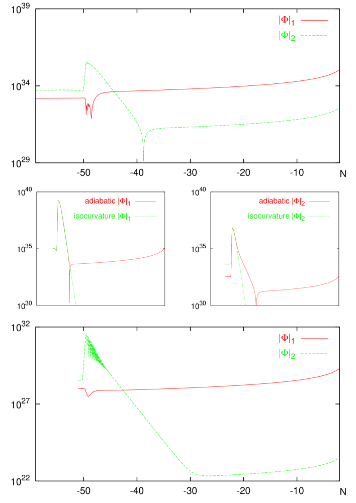
Figure 1: Evolution of the metric perturbations, when Higgs perturbations are neglected : (top) $|\Phi_{1}|$ and $|\Phi_{2}|$ for a long wavelength mode; (middle left) splitting of $|\Phi_{1}|$ in adiabatic and isocurvature contributions for this mode; (middle right) same for $|\Phi_{2}|$; (bottom) $|\Phi_{1}|$ and $|\Phi_{2}|$ for a small wavelength mode. The transition starts at $N_{c}\simeq-50$, while the last inflationary stage ends at $N\simeq 0$. The long wavelength mode exits the Hubble radius at $N=-53$, the small wavelength mode at $N=-44$.

We integrate the equations for a mode that crosses the Hubble radius around $N=-53$, while $N_{c}=-50$ (the origin for $N$ has been chosen so that the last inflationary stage ends at $N=0$). The results for $|\Phi_{1}|$ and $|\Phi_{2}|$ are shown on the first plot of fig.1. Since the final power spectrum will depend on the final value of $|\Phi_{1}|$, which is much bigger than $|\Phi_{2}|$ during the last stage, it is important to understand the evolution of this quantity, and to compare with slow-roll predictions.

In first approximation, the evolution of $\Phi_{1}$ can be reproduced analytically. Indeed, we check that the perturbation $\delta B_{1}$, though amplified exponentially during the transition, remains a negligible source term for $\Phi_{1}$ and $\delta A_{1}$, except during a short period (two $e$-folds) during which it is comparable with other source terms. So, at first order, we can just neglect $\delta B_{1}$, and deduce the evolution of $\Phi_{1}$ and $\delta A_{1}$ from a system of two differential equations instead of three.. Moreover, we look only for the slowly-varying solution, which obeys to :

$$3H\delta\dot{A}_{1}+\frac{\partial^{2}V}{\partial A^{2}}\delta A_{1}=-2\frac{\partial V}{\partial A}\Phi_{1},\qquad H\Phi_{1}=\frac{\dot{\bar{A}}\;\delta A_{1}}{2m_{P}^{2}}.$$ (23)

There is an exact solution (normalized to $|\delta A_{1}|=\frac{H}{\sqrt{2k^{3}}}$ at $t=t_{k}$), that reproduces fairly well the numerical solution :

$$\delta A_{1} = \frac{\dot{\bar{A}}}{\dot{\bar{A}}(t_{k})}\frac{H}{\sqrt{2k^{3}}}\exp\int_{t_{k}}^{t}\frac{\dot{\bar{A}}^{2}}{m_{P}^{2}H}dt,$$

$$\Phi_{1} = \frac{\dot{\bar{A}}^{2}}{\dot{\bar{A}}(t_{k})}\frac{1}{2\sqrt{2k^{3}}}\exp\int_{t_{k}}^{t}\frac{\dot{\bar{A}}^{2}}{m_{P}^{2}H}dt.$$ (24)

We must keep in mind that between $t_{c}$ and some time $t_{1}$, one has $\dot{\bar{B}}^{2}+\dot{\bar{C}}^{2}\geq\dot{\bar{A}}^{2}$ (this is the 15 $e$-fold “second stage with oscillations”). On the other hand, during the “second stage with slow-roll”, we have $2m_{P}^{2}\dot{H}=-\dot{\bar{A}}^{2}$, and eqs.(24) read :

$$\delta A_{1} = {\cal C}_{1}\frac{\dot{\bar{A}}}{H},\qquad\Phi_{1}=-{\cal C}_{1}\frac{\dot{H}}{H^{2}},$$

$${\cal C}_{1} = \frac{H(t_{k})}{m_{P}^{2}\sqrt{2k^{3}}}\frac{V(t_{k})}{\frac{\partial V}{\partial A}(t_{k})}\exp\int_{t_{k}}^{t}-\frac{\dot{\bar{B}}^{2}+\dot{\bar{C}}^{2}}{m_{P}^{2}H}dt.$$ (25)

Now, since the contribution to the last integral is made essentially for $t_{c}<t<t_{1}$ with $\dot{H}\simeq-\frac{\dot{\bar{B}}^{2}+\dot{\bar{C}}^{2}}{2m_{P}^{2}}$, the last term with the exponential can be approximated by $H^{2}(t_{1})/H^{2}(t_{k})$, and then :

$${\cal C}_{1}\simeq\frac{H(t_{k})}{m_{P}^{2}\sqrt{2k^{3}}}\frac{V(t_{1})}{\frac{\partial V}{\partial A}(t_{k})}.$$ (26)

This approached result matches exactly the slow-roll prediction (15), because $V(t_{1})$ is nothing else but $V_{A}$. In fact, we find that the numerical result (which takes into account the exact relation $-2m_{P}^{2}\dot{H}=\dot{\bar{A}}^{2}+\dot{\bar{B}}^{2}+\dot{\bar{C}}^{2}$, and the small correction due to the fact that $\delta B_{1}$ cannot be neglected during two $e$-folds) exceeds the slow-roll prediction by a factor 4.3.

To conclude on the evolution of $\Phi_{1}$, note that it is possible in principle to isolate numerically the adiabatic and the isocurvature contribution. We subtract to $\Phi_{1}$ a solution of the type of eq.(9), and also, a solution $\tilde{\cal D}/a$. We tune (${\cal C}_{1},\tilde{\cal C}_{1},\tilde{\cal D}$) in order to remove any behavior proportional to $1/a$ or $H/a$, and to cancel $\Phi_{1}$ during the second slow-roll stage. The result is unique and stands for the isocurvature mode. The second plot of Fig. 1 shows the result of this decomposition. At the end of this formal exercise, $\Phi_{1}$ appears as the result of an almost exact cancellation during the first stage between adiabatic and isocurvature contributions, which are of opposite sign. We see that both modes are excited during the transition, but the isocurvature mode decays like $a^{-3}$ during the second stage and vanishes.

On the other hand, the solution for $j=2$ differs completely from the standard slow-roll prediction. We expect from eqs.(15, 18, 22) that ${\cal C}_{2}\sim 3{\cal C}_{1}$. It is in fact $10^{3}$ times smaller. Again, this result shows that the usual definition of ($V_{A}$, $V_{B}$) is not valid during and before the slow-roll interruption. This appears clearly when we separate numerically the adiabatic and isocurvature contribution (third plot of fig.1). We see that during the first stage, the isocurvature mode completely dominates.

In conclusion, even if ${\cal C}=({\cal C}_{1}^{2}+{\cal C}_{2}^{2})^{1/2}$ differs from the slow-roll prediction only by a factor of order one, we have proved that the usual results of eqs.(14, 15) cannot be employed in our model. The numerical results can be matched with eqs.(13, 15) by tuning $V_{A}$ and $V_{B}$ during the first stage, but we don’t know how to predict these values analytically : this calculation seems to be difficult, and a numerical simulation is probably unavoidable.

3.2 Small wavelength result

We now consider the modes that cross the Hubble radius well after the transition. For the smallest wavelengths, this happens during the last single-field slow-roll stage, and the usual results of eqs.(15, 18, 22) are automatically valid. In our model, these modes correspond to very small wavelengths today, not observable on cosmic scales.

We are more interested in modes crossing the Hubble radius during the oscillatory period, when the evolution of $H$ is driven by $\dot{\bar{B}}^{2}\gg\dot{\bar{A}}^{2}$. The evolution of $(\Phi_{1},\Phi_{2})$ for such a mode, with Hubble crossing at $N\simeq-44$ (six $e$-folds after $N_{c}$), is shown on the last plot of fig.1. Since we are now in single-field inflation, $\Phi_{1}$ and $\Phi_{2}$ should be pure adiabatic modes; we check that this is the case, by fitting ($\Phi_{1}$, $\Phi_{2}$) with the expression of eq.(9) (for $N>-44$). The coefficient ${\cal C}_{1}$ matches exactly the slow-roll analytic prediction, and ${\cal C}_{2}\ll{\cal C}_{1}$, as expected for a non-slow-rolling field perturbation.

This can be explained easily. During the transition, $\Phi_{1}$ remains a slowly-varying solution, because the effective mass of $\delta A_{1}$ is dominated by $k^{2}/a^{2}$. So, at Hubble crossing, $\Phi_{1}$ is in the slowly-varying adiabatic mode, and ${\cal C}_{1}$ is exactly the same as in the slow-roll prediction (i.e. eq.(15) with $i=1$). On the other hand, $|\Phi_{2}|$ is strongly affected by the transition, because the effective mass of $\delta B_{2}$ becomes suddenly much larger than $k^{2}/a^{2}$. At Hubble crossing, $|\Phi_{2}|$ is in the decaying adiabatic mode, proportional to $a^{-1}$, and stabilize with a value much smaller than $|\Phi_{1}|$, as expected for a non slow-rolling field perturbation in single-field inflation.

3.3 Primordial power spectrum

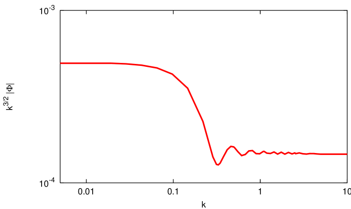
Figure 2: The primordial power spectrum of adiabatic fluctuations, $k^{3/2}{\cal C}(k)$, or equivalently, $k^{3/2}|\Phi(k)|$, when the Higgs perturbations are neglected (with logarithmic scale and arbitrary units). It is a step-like spectrum with superimposed oscillations on intermediate scales.

We plot on fig.2 the power spectrum of adiabatic fluctuations, $k^{3/2}{\cal C}(k)$, or equivalently (up to a constant), $k^{3/2}\Phi(k)$. It is a step-like spectrum with superimposed oscillations on small scales, quite similar to the analytic spectrum of Starobinsky [18], but more smooth (the amplitude of the first oscillations with respect to the amplitude of the step is smaller). On intermediate and small scales, it is also close to the spectrum of [9] (from double “polynomial” inflation), with the notable difference that on large scale we have an approximately flat plateau, instead of a logarithmic dependence on $k$.

For our choice of primordial parameters, the step has got an amplitude $p\simeq 10$, and spans over one decade in $k$ space. As we saw before, this spectrum arises solely from ${\cal C}_{1}$, i.e., from metric perturbations calculated with initial condition of the type ($\delta A\neq 0$, $\delta B=0$).

4 Dynamics of the Higgs field

Until now, we have treated the Higgs field $C$ as a simple classical homogeneous background field, and put by hand an initial condition at $N=N_{c}$, in order to push the field away from unstable equilibrium. We will now enter into more details concerning the Higgs quantum fluctuations, in order to justify and calculate the initial condition at $N_{c}$ (by averaging over quantum fluctuations), and to prepare the work of the following section, in which we will consider the effect of the Higgs quantum perturbations on the primordial power spectrum. We rewrite the potential (Appendix, eq.(48)) under the more suggestive form :

$$V=V(A,B)+\frac{1}{4}\beta^{2}(B^{2}-B_{c}^{2})C^{2}+\frac{\beta^{2}B_{c}^{2}}{8C_{eq}^{2}}C^{4}.$$ (27)

When $B<B_{c}$, the potential is a usual “Mexican hat” with respect to $C$.

4.1 Fluctuations during the first stage of inflation

We decompose the field $C$ as in eqs.(1,2), using now a three-dimensional operator basis $\hat{a}_{j,~{}j=1,2,3}$. Since $C$ is complex, we would need in principle a four-dimensional basis, in order to quantify separately the real and imaginary part $C_{1}$ and $C_{2}$. However, in this section, the $U(1)$ symmetry will still be preserved, and the mode functions are identical for $C_{1}$ and $C_{2}$. So, for concision, we introduce only one degree of freedom $j=3$, describing simultaneously both directions in the complex plane.

The Wronskian condition (3) applies also to the mode function $\delta C_{j}$. During the first stage of inflation, $\bar{C}=0$. So, in addition to eqs.(16) (now taken for $j=1,2,3$), we have the following perturbation equation :

$$\ddot{\delta C_{j}}+3H\dot{\delta C_{j}}+\left(\frac{k^{2}}{a^{2}}+\frac{\partial^{2}V}{\partial C^{2}}\right)\delta C_{j}=0,$$ (28)

with a WKB solution valid both within and outside the Hubble radius :

$$\delta C_{j} = \delta_{3j}\frac{a^{-3/2}}{\sqrt{2m}}e^{-i\int mdt},$$ (29)

$${\rm with}\qquad m^{2} \equiv \frac{k^{2}}{a^{2}}+\frac{\partial^{2}V}{\partial C^{2}}-\frac{9}{4}H^{2}.$$

During the first stage of inflation, at the first perturbative order considered here, $\Phi_{3}$ vanishes, and so do the non-diagonal mode functions ($\delta A_{3}$, $\delta B_{3}$, $\delta C_{j\neq 3}$). $\delta C_{3}$ is decoupled from other perturbations and its evolution depends mainly on the mass $\partial^{2}V/\partial C^{2}=\frac{1}{2}\beta^{2}(B^{2}-B_{c}^{2})$ that goes to zero at $N=N_{c}$.

4.2 Formation of inhomogeneities just after $N_{c}$

When $N>N_{c}$, the mass of $C$ becomes negative, causing an exponential amplification of the mode functions, known as spinodal instability. Let us restrict the analysis to the very short stage after $N_{c}$, during which $\delta C_{3}$ remain small enough for the linear equation (28) to be still valid. As we can check a posteriori, this stage lasts $\sim 0.15$ $e$-folds. If we re-scale $\delta C_{3}$ to $\chi\equiv a^{3/2}\delta C_{3}$, we see that eq. (28) can be rewritten :

$$\ddot{\chi}+\left(\frac{k^{2}}{a^{2}}+\frac{\partial^{2}V}{\partial C^{2}}-\frac{9}{4}H^{2}\right)\chi=0.$$ (30)

We will solve this equation under a few approximations, and compare our result with an exact numerical simulation. Since we are interested in a short period after $N_{c}$, with typically $N-N_{c}\leq 0.2$, it is appropriate to linearize the $N$-dependence of the effective mass-term in equation (30) :

$$\frac{\partial^{2}V}{\partial C^{2}} = -\mu^{2}(N-N_{c}),\qquad\mu^{2}\equiv-\left.\frac{d\{\partial^{2}V/\partial C^{2}\}}{dN}\right|_{N_{c}}>0,$$ (31)

$$\frac{k^{2}}{a^{2}} = \frac{k^{2}}{a_{c}^{2}}(1-2(N-N_{c}))$$

(in the particular model we are studying, $\mu$ can be easily found from the slow-roll condition for $\bar{B}$ : $\mu^{2}=\frac{\beta^{2}B}{3H^{2}}\frac{\partial V}{\partial B}=\frac{\beta^{2}}{3H^{2}}\frac{2\ln 2(g_{A}^{2}\xi_{A}+g_{B}^{2}\xi_{B})^{2}}{16\pi^{2}}$). Also, during this short stage, $H$ is approximately constant and $N-N_{c}=H(t-t_{c})$. Under these approximations, equation (30) reads :

$$\ddot{\chi}-\mu_{k}^{2}\;H\;(t-t_{k})\;\chi=0,$$ (32)

with :

$$\mu_{k}^{2}=\mu^{2}+2\frac{k^{2}}{a_{c}^{2}},\qquad t_{k}=t_{c}+\frac{1}{\mu_{k}^{2}H}\left(\frac{k^{2}}{a_{c}^{2}}-\frac{9}{4}H^{2}\right).$$

The modes $\chi$ start growing exponentially at $t=t_{k}$ (for $k=0$, $t=t_{c}-\frac{9H}{4\mu^{2}}$, but smaller wavelengths start growing later). The correctly normalized solution of equations (32) and (28) is given, up to an arbitrary complex phase, by :

$$\chi = \sqrt{\frac{\pi}{6}}(t-t_{k})^{1/2}~{}{\cal H}^{(1)}_{1/3}\!\left[\frac{2i}{3}\mu_{k}H^{1/2}(t-t_{k})^{3/2}\right],$$ (33)

$$\delta C_{3} = a^{-3/2}\chi,$$

where ${\cal H}^{(1)}_{1/3}[z]$ is a Hankel function of the first kind. Indeed, for $t<t_{k}$, this solution has an asymptotic expression which is identical to equation (29). For $t\simeq t_{k}$, one has :

$$\delta C_{3}=a^{-3/2}\frac{\sqrt{2\pi}}{3\Gamma(\frac{2}{3})}\left(\frac{3}{\mu_{k}H^{1/2}}\right)^{1/3},$$ (34)

and for $t>t_{k}$ in very good approximation :

$$\delta C_{3}=a^{-3/2}\frac{\exp\left(\frac{2}{3}\mu_{k}H^{1/2}(t-t_{k})^{3/2}\right)}{\sqrt{2\mu_{k}H^{1/2}(t-t_{k})^{1/2}}}.$$ (35)

Is it possible to define an effective background from the coarse-graining of long wavelength modes? The field $C$, coarse-grained over a patch of size $l\sim 2\pi a/k$, is a stochastic classical quantity. Its real and imaginary part obey to a Gaussian distribution (at least if all modes are in the vacuum state), with variance $<\!\bar{C}^{2}\!>^{1/2}$ computed from :

$$<\!\bar{C}^{2}\!> \equiv \int_{0}^{k_{cg}}\!\!\!\int\frac{d^{3}{\bf k}~{}d^{3}{\bf k}^{\prime}}{(2\pi)^{3}}\langle 0|\delta C({\bf k},{\bf x},t)\delta C^{\dagger}({\bf k^{\prime}},{\bf x},t)|0\rangle$$ (38)

$$= \frac{1}{2\pi^{2}}\int_{0}^{k_{cg}}k^{2}\left|\delta C_{3}\right|^{2}dk,$$

where $k_{cg}$ is the coarse-graining cut-off. When $t<t_{c}$, we know that scales outside and around the Hubble radius have a $k$-independent amplitude (see eq.(29)). So, $<\!\bar{C}^{2}\!>$ scales like $k_{cg}^{3}$ (intuitively, all modes have the same amplitude, but small wavelength have a bigger statistical weight, proportional to $k^{2}$). On the other hand, when $t\geq t_{c}$, large wavelengths start being amplified earlier; so, in the coarse-graining integral, there is a competition between the term $|\delta C_{3}|^{2}$ and the term $k^{2}$, and a scale will be privileged. More precisely, let us use the asymptotic expression (35). The function $k^{2}|\delta C_{3}|^{2}$ peaks around the scale

$$k_{max}=a_{c}\left(\frac{\mu H}{2\sqrt{N-N_{c}}}\right)^{1/2},$$ (39)

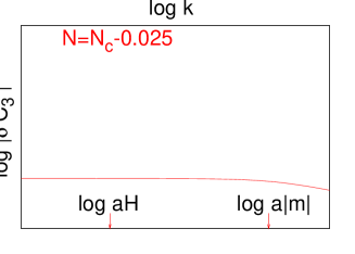
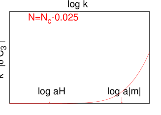
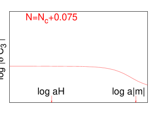
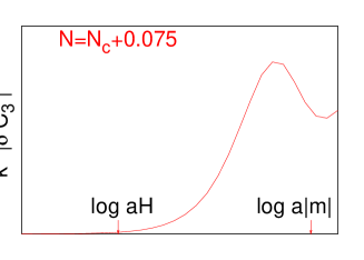
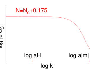
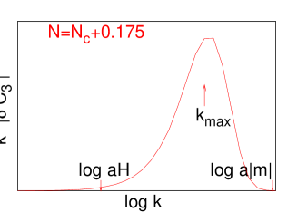
Figure 3: The left column shows the Higgs perturbation power spectrum : $\log|\delta C_{3}|^{2}$ versus $\log k$, for different times chosen around the beginning of the transition, i.e, when the effective mass of $C$ becomes negative. From top to bottom, we have $N-N_{c}=-0.025,0.075,0.175$. The vertical scale is the same in the three plots. We show on the horizontal axis the particular values corresponding to $k=aH$ and $k=a|m|$, where $m^{2}\equiv\partial^{2}V/\partial C^{2}$. We see that spinodal modes, with $k\leq a|m|$, are amplified.    On the right column, we plot the integrand of the coarse-graining integral : $k^{2}|\delta C_{3}|^{2}$. The vertical scale increases from top to bottom. It appears clearly that after a fraction of $e$-fold, only modes with $H<k/a<|m|$ contribute to this integral, which indicates the emergence of an inhomogeneous background, with first-order homogeneity recovered on smaller scales (higher $k$). On the last plot, we also show the scale $k_{max}$ calculated analytically from eq.(39).

and only modes in the range $0.1k_{max}<k<3k_{max}$, which are within the Hubble radius, contribute to the coarse-graining integral (38). A numerical simulation confirms this result for $0.1\leq N-N_{c}\leq 0.2$ (see fig.3). This means that just after $N_{c}$, the field $C$ has an inhomogeneous structure, and can be seen as effectively homogeneous only in regions of typical size $\lambda\ll a/k_{max}$.

Inside each patch, we can define an effective homogeneous background from the coarse-graining of large wavelength modes, and use the standard semi-classical approximation. The constant phase in a given patch can be chosen randomly, while the squared modulus $|\bar{C}|$ obeys a probability distribution that can be calculated exactly. Indeed, with any coarse-graining cut-off $k_{cg}\sim 3k_{max}$, we can compute the root mean square of the real and imaginary part of $C$ :

$$<\!\bar{C}^{2}\!>^{1/2}=\frac{1}{4\pi^{3/2}}\left(\frac{a_{c}}{a}\right)^{3/2}\left(\frac{\mu_{0}^{2}H}{t-t_{c}}\right)^{1/4}\exp\left(\frac{2}{3}\mu H^{1/2}(t-t_{c})^{3/2}\right).$$ (40)

Since $C_{1}$ and $C_{2}$ are Gaussian stochastic numbers with variance $<\!\bar{C}^{2}\!>^{1/2}$, then $|C|^{2}$ obeys a $\chi^{2}$ distribution and $|C|$ has a mean value $\simeq\sqrt{3/2}<\!\bar{C}^{2}\!>^{1/2}$ and a variance $\simeq\sqrt{1/2}<\!\bar{C}^{2}\!>^{1/2}$ (the numerical factors can be found in tables; see, for instance, eq.(26.4.34) in [42]). We see explicitly, by comparing with eqs.(34, 35), that $<\!\bar{C}^{2}\!>^{1/2}$ is a solution of the zero-mode equation with initial condition : $<\!\bar{C}^{2}\!>^{1/2}(t_{c})=(6\pi\Gamma(\frac{2}{3}))^{-1}(3\mu^{2}H)^{1/3}$. Actually, the numerical simulation shows that the exact result exceeds this estimate by a factor 2.3, so that the correct initial condition is :

$$<\!\bar{C}^{2}\!>^{1/2}(t_{c})=0.12~{}(\mu^{2}H)^{1/3}.$$ (41)

So, we really have in each patch an effective homogeneous background, obeying for $N\geq 0.1$ to the equation $\ddot{\bar{C}}+3H\dot{\bar{C}}+\partial V/\partial C=0$, and with an initial $\chi^{2}$ distribution of probability.

On the other hand, on scales $k\leq k_{max}$, the background is essentially inhomogeneous, and due to strong mode-mode coupling, the linear semi-classical approximation breaks soon after $N_{c}$.

4.3 Later evolution and the homogeneous phase approximation

So, it is not possible to find an exact solution for the evolution of $C$ during spinodal instability and at later time. We should recall here that out-of-equilibrium phase transitions and spinodal instability have been widely studied in condensed matter physics, and also in the context of “spinodal inflation”, using either the large-N limit [31, 32] (which is well-defined, but appropriate for the symmetry breaking of $U(N)$, $N\rightarrow\infty$), or just a Hartree-Fock approximation [33] (which is more difficult to interpret, and cannot account so far for the metric back-reaction). In such studies, the typical scale of homogeneity for the coarse-grained background is larger than the Hubble radius ($k_{max}<a(t_{c})H(t_{c})$), while the observable primordial spectrum arises from modes with $k>a(t_{c})H(t_{c})$. So, it is possible to separate completely the modes contributing to the “effective zero-mode assembly”, and those contributing to the primordial spectrum. In contrast, in our case, we need to follow modes on scales $k$ with $k<a(t_{c})H(t_{c})<k_{max}$. So, at first sight, it seems that our problem is much more complicated than spinodal inflation, due to the inhomogeneity of the background. In fact, it is not, because we have an inflaton field $A$ driving inflation even during the transition, and we will see that a perturbative semi-classical approach can still be employed.

The following observations will suggest an approximation under which we can continue the primordial spectrum calculation :

• since the causal horizon during the first inflationary stage is much bigger than the Hubble radius, ($A$, $B$) are homogeneous on the largest scales observable today, $B_{c}$ is reached everywhere at the same time, and the phase transition is triggered coherently. So, the modulus $|C|$ should be approximately homogeneous, even on the largest scales : we should be able to cast it into a zero-mode plus small perturbations.

• the phase inhomogeneities should not be much relevant for the primordial spectrum calculation. The existence of a negative mass, leading to exponential amplification, only arise in the longitudinal direction $|C|$. The degree of freedom associated with the complex phase is a Goldstone boson; it is eaten up by the gauge field, which becomes massive. Starting from zero, this mass soon exceeds the Hubble parameter : so, there cannot be large quantum fluctuations arising from this sector. The existence of phase inhomogeneities is also linked to the formation of cosmic strings at the very beginning of spontaneous symmetry breaking, separated at least by a characteristic length $\lambda>a/k_{max}$. These strings could eventually contribute to the formation of cosmological perturbations today, but as we said in the introduction, we do not include such mechanism in this study.

So, for our purpose, it seems reasonable to neglect the phase inhomogeneities, forget the vacuum degeneracy, and assume a homogeneous phase $\theta({\bf x},t)=\bar{\theta}$. In the following section, we will recompute the primordial power spectrum, taking now into account the Higgs longitudinal quantum perturbations, and we will find that these perturbations have a characteristic signature on the primordial power spectrum.

5 Spectrum with Higgs longitudinal perturbations

We go on neglecting the vacuum degeneracy. We saw in section 4.2 that just after the transition, the modulus $|C|$ has got a mean value $\sqrt{3/2}<\!|C|^{2}\!>^{1/2}$ and a variance $\sqrt{1/2}<\!|C|^{2}\!>^{1/2}$ that we calculated explicitly. Assuming a homogeneous phase is almost equivalent to identifying this modulus with a real scalar field, canonically quantized, and decomposed, following the usual semi-classical approximation, into a background field $\bar{C}=\sqrt{3/2}<\!|C|^{2}\!>^{1/2}$, plus quantum fluctuations. The quantum mode functions should be matched with the quantities $\delta C_{j}$ that we already studied around $N_{c}$, divided by $\sqrt{2}$. With these prescriptions, the mean value and the variance of the modulus previously studied in the last section coincide exactly with those of the real scalar field introduced in this paragraph.

This matching is the key point of our study. It is not exact, because, in a classical stochastic sense, it is based only on the first two momenta of the $\chi^{2}$ distribution : we artificially “gaussianize” the fluctuations. However, the matching seems appropriate for estimating the amplitude of the quantum fluctuations of the modulus $|C|$, even if any information on a possible non-gaussianity is lost. Since in this approach we introduce a (physically justified) zero-mode, we expect that the growth of spinodal modes will slow-down and terminate rapidly, and that the perturbative semi-classical approach will remain valid. This will be justified explicitly in section 5.3.

In summary, we simulate the usual background equations for ($\bar{A}$, $\bar{B}$, $\bar{C}$, $H$) and the following perturbation equations :

$$\ddot{\delta A_{j}}+3H\dot{\delta A_{j}}+\left(\frac{k^{2}}{a^{2}}+\frac{\partial^{2}V}{\partial A^{2}}\right)\delta A_{j} = 4\dot{\bar{A}}\dot{\Phi}_{j}-2\frac{\partial V}{\partial A}\Phi_{j}-\frac{\partial^{2}V}{\partial A\partial B}\delta B_{j},$$

$$\ddot{\delta B_{j}}+3H\dot{\delta B_{j}}+\left(\frac{k^{2}}{a^{2}}+\frac{\partial^{2}V}{\partial B^{2}}\right)\delta B_{j} = 4\dot{\bar{B}}\dot{\Phi}_{j}-2\frac{\partial V}{\partial B}\Phi_{j}-\frac{\partial^{2}V}{\partial A\partial B}\delta A_{j}-\frac{\partial^{2}V}{\partial B\partial C}\delta C_{j},$$

$$\ddot{\delta C_{j}}+3H\dot{\delta C_{j}}+\left(\frac{k^{2}}{a^{2}}+\frac{\partial^{2}V}{\partial C^{2}}\right)\delta C_{j} = 4\dot{\bar{C}}\dot{\Phi}_{j}-2\frac{\partial V}{\partial C}\Phi_{j}-\frac{\partial^{2}V}{\partial B\partial C}\delta B_{j},$$

$$\dot{\Phi}_{j}+H\Phi_{j} = \frac{1}{2m_{P}^{2}}(\dot{\bar{A}}\delta A_{j}+\dot{\bar{B}}\delta B_{j}+\dot{\bar{C}}\delta C_{j}).$$ (42)

When we start following a mode $\delta C_{j}$ well inside the Hubble radius, we employ the initial condition of eq.(29) divided by a factor $\sqrt{2}$. At $N=N_{c}$, we put by hand a non zero-value for $\bar{C}$, given by eq.(41) multiplied by a factor $\sqrt{3/2}$.

5.1 Large wavelength results

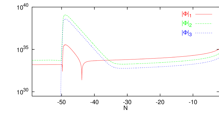
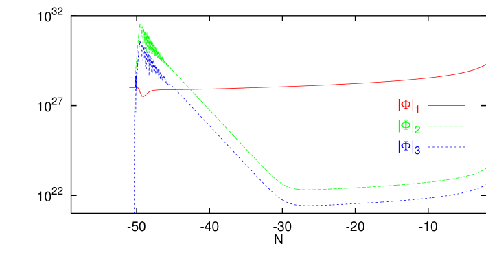
Figure 4: We now take into account the Higgs longitudinal perturbations, and show the evolution of the metric perturbations ($|\Phi_{1}|$, $|\Phi_{2}|$, $|\Phi_{3}|$), for (top) a long wavelength mode, crossing the Hubble radius at $N=-53$, and (bottom) a small wavelength mode, crossing at $N=-43$.

The evolution of ($|\Phi_{1}|$, $|\Phi_{2}|$, $|\Phi_{3}|$) for a mode crossing the Hubble radius at $N\simeq-53$ (i.e. during the oscillatory stage) is shown on the upper plot of fig.4. By subtracting the previous solution (fig.1) to the new solution (fig.4), we check that the evolution of $|\Phi_{1}|$ is unchanged, except during a few $e$-folds after the beginning of the transition. The difference is due to the small (one-loop) coupling term $\frac{\partial^{2}V}{\partial A\partial B}$ : when $\delta B_{1}$ is amplified, it excites $|\Phi_{1}|$, but later on, this mode decays and doesn’t leave an observable signature. On the other hand, the negative effective mass of $\delta C_{j}$ and the large (tree-level) coupling between $\delta B_{j}$ and $\delta C_{j}$ generate a considerable amplification of $|\Phi_{2}|$ and $|\Phi_{3}|$. At the end, when the isocurvature modes and the decaying adiabatic mode can be neglected, the remaining growing adiabatic mode is smaller than the one for $|\Phi_{1}|$, but only by one order of magnitude.

So, on large scale, what is the observable difference between these results, and those of section 3 ? First, since initial conditions for $\delta B_{2}$ are proportional to $(a\sqrt{k})^{-1}$, we expect the large-scale power spectrum for $k^{3/2}|\Phi_{2}|$ to be, as usual, approximately scale-invariant. In other words, the contribution found for one mode will be the same for other large-scale modes. So, the large-scale power spectrum will still be a flat plateau, but possibly with a small deviation from gaussianity, caused by the small contribution of $|\Phi_{2}|$. As we said before, our method does not allow a quantitative evaluation of this deviation, and we leave this for further studies. Second, since initial conditions for $\delta C_{3}$ are independent of the scale, and since the factor $k^{2}/a^{2}$ is always sub-dominant in the effective mass of $\delta C_{3}$ on large wavelengths, $|\Phi_{3}|$ should be scale-independent on these wavelengths. So, the contribution of $k^{3/2}|\Phi_{3}|$ to the power spectrum $k^{3/2}<|\Phi|^{2}>^{1/2}$ will be proportional to $k^{3/2}$, and will peak for scales crossing the Hubble length during the transition. We therefore expect an observable non-Gaussian spike, whose shape and amplitude will be calculated in section 5.4.

5.2 Small wavelength result

The evolution of ($|\Phi_{1}|$, $|\Phi_{2}|$, $|\Phi_{3}|$), for a mode crossing the Hubble radius at $N\simeq-43$ (i.e. during the oscillatory stage), is shown on the lower plot of fig.4. $|\Phi_{1}|$ and $|\Phi_{2}|$ are identical to previous results of section 3.2. $|\Phi_{3}|$ has the same behavior as $|\Phi_{2}|$, but is even smaller. So, for small wavelengths, including the Higgs modulus perturbation makes no difference at all.

5.3 Consistency check of the semi-classical approximation

Before giving the primordial spectrum of perturbations, we will check here the consistency of our approach, and the validity of the semi-classical approximation in our case. Strictly speaking, the semi-classical approximation holds whenever for each field, the Klein-Gordon equation

$$g^{-1/2}\partial_{\mu}(g^{1/2}g^{\mu\nu}\partial_{\nu}\varphi({\bf x},t))+\frac{\partial V}{\partial\varphi}\left(\varphi({\bf x},t)\right)=0$$ (43)

can be casted into a background equation for the zero-mode, plus independent linear equations for field and metric mode functions. The first term, with space-time derivatives, is linear provided that metric perturbations remain small :

$$<\!0|~{}|\int\frac{d^{3}{\bf k}}{(2\pi)^{3/2}}\Phi|^{2}|0\!>^{1/2}\ll 1.$$ (44)

The second term, with the potential derivative, is linear in two cases :

1. obviously, when the perturbations are small with respect to the zero-mode :
   $<\!0|~{}|\int\frac{d^{3}{\bf k}}{(2\pi)^{3/2}}\delta\varphi|^{2}|0\!>^{1/2}\ll\bar{\varphi}$. Then, we can write :

   $$\frac{\partial V}{\partial\varphi}\left(\varphi({\bf x},t)\right)\simeq\frac{\partial V}{\partial\varphi}(\bar{\varphi})\;+\;\frac{\partial^{2}V}{\partial\varphi^{2}}(\bar{\varphi})~{}\times~{}\int\frac{d^{3}{\bf k}}{(2\pi)^{3/2}}\delta\varphi.$$ (45)

2. also, when both the zero-mode and the perturbation expectation value are small enough for non-quadratic terms in the potential to be neglected. Then, we have the following linearization :

   $$\frac{\partial V}{\partial\varphi}\left(\varphi({\bf x},t)\right)=\frac{\partial^{2}V}{\partial\varphi^{2}}\times\varphi({\bf x},t),$$ (46)

   and $\partial^{2}V/\partial\varphi^{2}$ is a constant.

We have seen that around $N=N_{c}+0.15$, in the homogeneous phase approximation, we can define a zero-mode and a set of perturbations. Since all these quantities are very small, we are in the second case, and the semi-classical approximation is valid. But what happens later? We know from figure 4 that one $e$-fold after $N_{c}$, the perturbations of $C$, $B$ and $\Phi$ reach a maximum; if, at that time, the expectation values of the perturbations exceed the homogeneous background fields (or, in the case of metric perturbation, exceed one), then our approach is simply inconsistent.

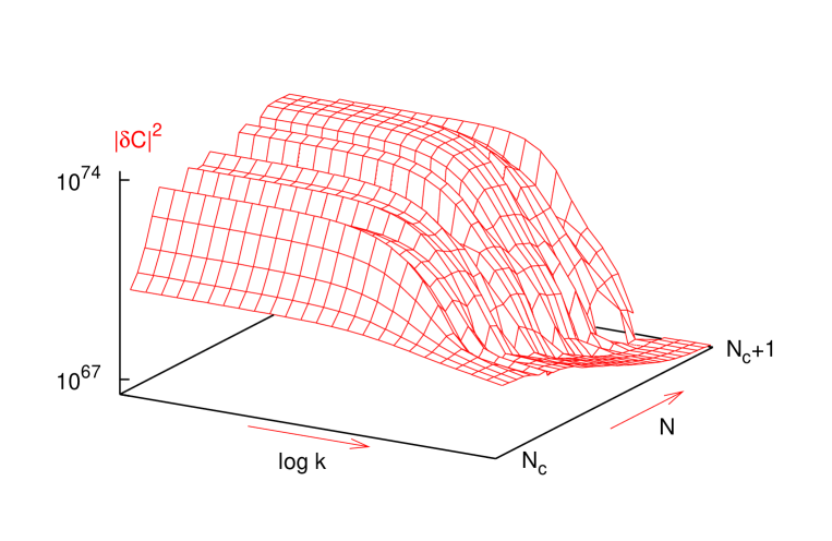
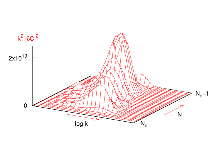
Figure 5: Before calculating the expectation value of quantum perturbations, and compare it with background quantities, it is useful to follow the various power spectra, plotted here for $\delta C$. The upper plot, $|\delta C|^{2}$ (logarithmic scale) versus $k$ and $N$, shows that spinodal modes are exponentially amplified, and then oscillate coherently. The second plot, $k^{2}|\delta C|^{2}$ (linear scale) versus $k$ and $N$, shows that the main contribution to the averaging integral arises always from the same modes, with $k\sim k_{max}$; this plot shows how to define the limits of integration in the averaging integral.

To address this question, we first study the evolution of the power spectra of $\delta C_{j}$, $\delta B_{j}$ and $\Phi_{j}$, for $N_{c}<N<N_{c}+1$. The results for $\delta C_{j}$ are shown on three-dimensional plots, in fig.5. This simulation is just the continuation of the one performed in section 4.2, and at low $N$ we recognize the curves of fig.3. On the upper plot, we show $\sum_{j}<|\delta C_{j}|^{2}>$, in logarithmic scale, vs. $k$ and $N$. We see that large scales (spinodal modes) are exponentially amplified during the spinodal stage, and then perform coherent oscillations, driven by the background evolution. On the lower plot, we show $k^{2}\sum_{j}<|\delta C_{j}|^{2}>$, in linear scale, vs. $k$ and $N$. We observe that the main contribution to the averaging integral (eq.(38)) always arise from the same region in $k$ space, centered around the approximately constant wavenumber $k_{max}$. This observation is technically important, because it justifies the use of finite limits of integration in the averaging integral. In particular, we see that we don’t have to worry with ultra-violet divergences. Provided that the upper limit of integration $k_{cut-of\!f}$ is chosen in a finite range (namely, around the largest $k$ values shown of fig.5), then $<|C|^{2}>$ does not depend on this cut-off. Similar results are found for $\delta B_{j}$ and $\Phi_{j}$.

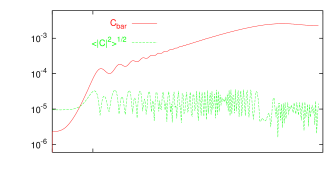
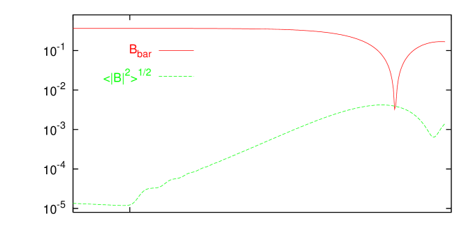
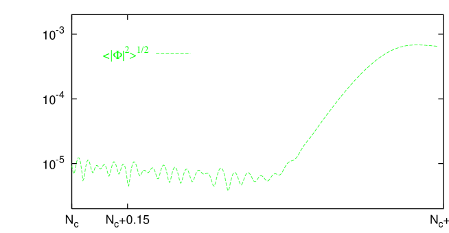
Figure 6: Consistency check of the semi-classical approximation. The expectation value of the quantum perturbations $<\!|\varphi|^{2}\!>^{1/2}$ is generally much smaller than the background fields $\bar{\varphi}$ (than one in the case of metric perturbations). When it is not the case, both quantities are very small and the linear approximation is still valid. The three plots correspond to the case of $C$, $B$, and $\Phi$. The case of $A$ is not shown because we know from the beginning that this field remains extremely homogeneous. The evolution is shown only until $N=N_{c}+1$, which is the time of maximal inhomogeneity, as can be seen on fig.4.

Then, by integrating on $k$, we find the expectation values $<|C|^{2}>^{1/2}$, $<|B|^{2}>^{1/2}$, $<|\Phi|^{2}>^{1/2}$, and plot them with respect to $\bar{C}$, $\bar{B}$ and $1$ (see fig.6). It appears that for $N\simeq N_{c}+0.20$, when $\bar{C}$ approaches the valley of minima (on the figure, we recognize this valley from the small oscillations around it), i.e., when $\partial V/\partial C$ becomes non-linear, the quantum perturbations are sub-dominant by one order of magnitude. When $\bar{C}$ reaches $C_{eq}$, the quantum expectation value is smaller by three orders of magnitude. After, we know from fig.4 that the field will become more and more homogeneous. For $B$, we see that the perturbations are always sub-dominant (when $\bar{B}$ performs its first oscillation, it goes through zero, but the perturbations are still quite small and we remain in the linear regime). For $\Phi$, the maximal value is $<|\Phi|^{2}>^{1/2}\sim 10^{-3}$. So, the semi-classical approach holds at any time in the range $N_{c}<N<N_{c}+1$, and therefore, until the end of inflation.

In conclusion, in this model, the semi-classical approximation can be employed during the whole evolution, because there exists a time ($N\simeq N_{c}+0.15$) at which the perturbations have grown sufficiently to create an effective zero-mode (obeying the usual zero-mode equation), but not too much, so that we are still in the linear region of the potential derivative. It is at this time that we have done the matching between the complex field (with no zero-mode) and a real scalar field (with a zero-mode) standing for its modulus. If such a time did not exist, complicated non-linear approaches and further approximations would have to be employed. This would be the case if the second inflaton field $A$ was not supplying a constant potential energy, and supporting the Universe expansion. Indeed, in that case, the evolution of the scale-factor and of the fields would become completely stochastic, and it would be a hopeless challenge to keep track of modes crossing the Hubble length before and during the transition.

5.4 Primordial spectrum including Higgs longitudinal perturbations

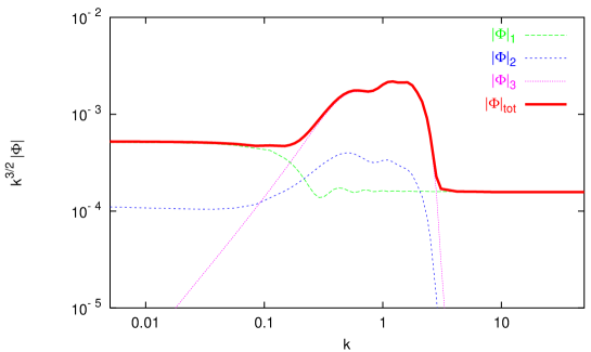
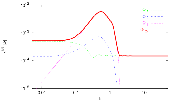
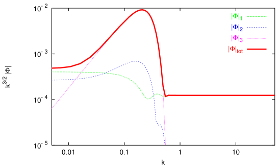
Figure 7: The primordial power spectrum of adiabatic fluctuations, $k^{3/2}{\cal C}(k)$, or equivalently, $k^{3/2}\Phi(k)$, when the Higgs longitudinal perturbations are taken into account (in logarithmic scale and arbitrary units). Together with the total power spectrum, we plot the three contributions from $\Phi_{j=1,2,3}$. For scales crossing the Hubble length during the phase transition, $\Phi_{3}$ produces a spike (possibly non-Gaussian). On the first three plots, the parameters $(\xi_{A},\xi_{B},g_{A},g_{B})$ are fixed to the values of the appendix, and $\beta=2\times 10^{-3}$ (top), $10^{-3}$ (middle), $0.5\times 10^{-3}$ (bottom).

We show our final result on figure 7, for the parameters used previously (middle). On the other plots, we show some primordial spectra corresponding to different values of $\beta$. The contribution of $|\Phi_{1}|$ is unchanged with respect to fig. 2, but we now have an additional contribution from $\Phi_{2}$ and $\Phi_{3}$ on intermediate and large scales. Let us summarize the characteristics of the power spectrum :

$\bullet$ On small scales (large $k$), we have an approximately flat plateau, exactly identical to the analytic predictions. Its amplitude can be found in our previous paper ([23], eqs. (6,7)), as a function of the Fayet-Illiopoulos terms ($\xi_{A}$, $\xi_{B}$), of the coupling constants ($g_{A}$, $g_{B}$) and of the duration of the second stage $\Delta N$ (different values of $\Delta N$ correspond to different choices for the inflaton fields initial values). The plateau has got a tilt $n_{S}=1-1/\Delta N\simeq 0.98$, like in usual (single-field) inflationary models, when the potential derivative is provided by logarithmic one-loop corrections.

$\bullet$ On intermediate scales (the value of these scales is given by $\Delta N$), we find a spike, as expected from sections 5.1 and 5.2 (since $k^{3/2}|\Phi_{3}|$ is proportional to $k^{3/2}$ for small $k$, and strongly suppressed for large $k$). This spike may be non-Gaussian, for reasons that we already explained. Clearly, it is beyond the scope of this paper to quantify the non-gaussianity, because the semi-classical approximation is not appropriate for extracting the statistics of the modes. The amplitude and width of this spike with respect to large scales depend essentially on $\beta$. Indeed, $\beta$ is proportional to the Higgs mass, and then, controls the duration of the transition : for low $\beta$ values, the transition is long, exponential amplification is enhanced, and the spike is higher. Its width is roughly of one decade in $k$ space (but, since $k^{3/2}|\Phi_{3}|$ is proportional to $k^{3/2}$ on large scales, small spikes are automatically more narrow). The shape of the spike around its maximum is slightly non-trivial, reflecting the first oscillations of the field $B$ around zero during the transition. It is reasonable to state that if the primordial power spectrum really possesses a spike (in the range in which this is still an open possibility, i.e., $0.1\times 10^{-2}h$Mpc${}^{-1}\leq k\leq 5\times 10^{-2}h$Mpc^-1), then its amplitude is already constrained by observations to be smaller than $\sim$10 (here, we define the amplitude as the ratio between the maximum value of $k^{3/2}|\Phi|$ and the one, for instance, of the large-scale plateau). This corresponds to the condition $\beta\geq 10^{-3}$.

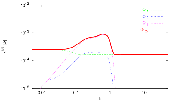
Figure 8: The primordial power spectrum of adiabatic fluctuations, for the same parameters as on fig.7 (upper plot), excepted lower values of $\xi_{A}$, $\xi_{B}$. On the right, the small scale plateau is unchanged, because we kept $\xi_{A}-\xi_{B}$ fixed. On the left, we get less power on large and intermediate scales.

$\bullet$ On large scales (small $k$), we also have an approximately flat plateau, but as we saw in section 3.1, we don’t know how to predict analytically the amplitude and tilt of this plateau, due to the violent slow-roll interruption during the transition. For our choice of parameters ($\xi_{A}$, $\xi_{B}$, $g_{A}$, $g_{B}$, $\Delta N$), there is a ratio of 4.3 between the amplitude obtained numerically for $k^{3/2}|\Phi|$, and the analytic prediction (eq.(13) of [23], or eq.(26) of this paper). This ratio is found to be approximately independent of $\beta$. The large scale tilt is very close to one. Finally, metric perturbations on these scales are composed of a (Gaussian) component $\Phi_{1}$, and of a (possibly non-Gaussian) component $\Phi_{2}$, generated, like $\Phi_{3}$, by the exponential amplification of perturbations during the transition. So, the relative contribution of $\Phi_{2}$ depends, like the spike, on $\beta$. For $\beta\geq 10^{-3}$, we find that $\Phi_{2}$ is sub-dominant, as can be seen in the figures, but not negligible (for $\beta=10^{-3}$, $|\Phi_{1}|/|\Phi_{2}|=3.4$). We also investigate the dependence of the large-scale plateau on $\xi_{A}$, $\xi_{B}$. Since small-scale amplitude depends on $\xi_{A}-\xi_{B}$ (see eq.(7) of [23]), we vary $\xi_{A}+\xi_{B}$ while keeping $\xi_{A}-\xi_{B}$ fixed. We find that the amplitude on large and intermediate scales increases with $\xi_{A}+\xi_{B}$. On fig.8, $\xi_{A}+\xi_{B}$ has been divided by 2.8, and other parameters are the same as in fig.7 (upper plot). In this case, the ratio between the two plateaus is 1.5.

6 Conclusion

We calculated numerically the primordial power spectrum for a particular model of double supersymmetric inflation, called double D-term inflation [23]. Following the usual semi-classical approach, we integrated for each independent mode function the equations of motion of field and scalar metric perturbations. Some technical difficulties (attached to any model of double hybrid inflation) arise between the two inflationary stages. Indeed, the first stage ends with a rapid second-order phase transition, taking place during inflation, and corresponding to the spontaneous symmetry breaking of a $U(1)$ gauge symmetry, triggered by a Higgs field $C$. This transition is followed by another inflationary stage, equivalent to usual hybrid inflation. We were especially interested in the behavior of modes exiting the Hubble radius during the transition, since they are expected to produce non-trivial features in the primordial power spectrum.

After spontaneous symmetry breaking, it is impossible to follow exactly the mode functions of the complex field $C$. Indeed, on the largest observable wavelengths, the complex phase of $C$ is completely inhomogeneous, at least at the beginning of the phase transition; so, on these scales, the usual perturbative semi-classical approach is broken by mode-mode coupling. However, we argued that only longitudinal Higgs perturbations, i.e., perturbations of $|C|$, can contribute to the primordial power spectrum. Indeed, these perturbations undergo a stage of spinodal instability, during which large wavelength modes are exponentially amplified, while the perturbations of the complex phase and of the gauge field (which combine into a massive gauge field, following the usual Higgs mechanism), are those of a non-slow-rolling field with large positive mass square.

So, we performed a calculation in which longitudinal Higgs perturbations are taken into account, with the modulus $|C|$ treated as an ordinary real scalar field, described by the semi-classical equations. We showed that at the beginning of the transition, a zero-mode for $|C|$ emerges from quantum fluctuations of $C$’s real and imaginary parts. Since the final result depends crucially on this initial zero-mode, we calculated it precisely in section 4.2. Then, by comparing the background fields and the averaged quantum perturbations, we showed that the semi-classical approach holds at any time. However, during one $e$-fold or so after the beginning of the transition, it is not far from its limits of validity (with typically a factor $10^{3}$ between background quantities and perturbations). This fact is a first hint that the contribution to the power spectrum resulting from longitudinal Higgs perturbations could be significantly non-Gaussian. The second hints comes from the fact that at the beginning of the transition, we identified a modulus with a real scalar field. In this process, we matched carefully the mean value and expectation value of both quantities, but information on higher momenta was lost. It is beyond the scope of this paper to evaluate the non-gaussianity.

Our final power spectrum, shown on fig.7 for different parameter values, can be divided in three regions :

1. a small-scale Gaussian plateau, whose amplitude and tilt ($n_{S}\simeq 0.98$) can be calculated analytically.

2. a possibly non-Gaussian spike, with an amplitude depending on the superpotential coupling parameter $\beta$. For $\beta\sim 10^{-3}$, the spike induces variations at most of order one in the primordial spectrum.

3. a large-scale plateau, for which we don’t have an exact analytic prediction. For $\beta\sim 10^{-3}$, deviations from gaussianity, if any, are expected to be small.

For a precise comparison of our model with CMB and large-scale-structure (LSS) data, one needs in principle, not only the primordial power spectrum of scalar adiabatic perturbations, but also the spectrum of primordial gravitational waves, and the contribution of cosmic strings formed during the two phase transitions (the one considered here, and the one occurring at the end of inflation). However, as we said in [23], the tensor-to-scalar ratio $T/S$ (for the first temperature anisotropy multipoles) depends essentially on the gauge coupling constants (as in single-field D-term inflation). Both $g_{A}$ and $g_{B}$ should be at most of order $10^{-1}$ (if not, inflation takes place with inflaton values of the order of the Planck mass, and supersymmetry/supergravity theories are not expected to be valid; see the Appendix for the consistency of this requirement with string theories). With this order of magnitude for the coupling constants, one can show easily that $T/S$ is negligible in double D-term inflation. On the other hand, cosmic strings can contribute significantly to the matter power spectrum and to CMB anisotropies, especially for D-term inflation, as shown in [27] (see also [28]). Since, in current studies, perturbations from strings and from the primordial spectrum are just added in quadrature, it is perfectly reasonable, at least in a first step, to calculate only the primordial spectrum. The ratio of strings-to-inflation large-scale temperature anisotropies, $R_{SI}=C_{5}^{S}/C_{5}^{I}$, is difficult to estimate; theoretical predictions give a ratio around 3 [27] or 4 [28], but the authors of this last reference argue that there are many uncertainties in these calculations, so that smaller values can still be considered seriously. With a mixture of inflationary and string perturbations, our model could still be interesting : the features would appear nevertheless, but smoothed by the cosmic string contribution.

In this work, we did not compare our results with CMB and LSS observations. Indeed, current data cannot distinguish with precision the kind of small features that we obtain, at least if they are located on scales $0.1\times 10^{-2}h$Mpc${}^{-1}\leq k\leq 5\times 10^{-2}h$Mpc^-1. However, as we said in the introduction, comparisons with observations of typical BSI spectra (with a step or a spike) have already been performed. The conclusions are currently quite encouraging (see for instance [17, 15]) and provide strong motivations for studying BSI inflationary models, until a final statement is made by future redshift surveys, such as the 2-degree Field project or the Sloan Digital Sky Survey, combined with forthcoming balloon and satellite CMB experiments.

An important qualitative aspect of our results is the possible deviation from gaussianity on intermediate and large scales. This may be related with the evidence for a non-gaussianity in the COBE data [28], but further work is needed on this point, since, on the one hand, we don’t have a precise theoretical prediction of non-gaussianity in this model, and on the other hand, the conclusion of [28] involves large uncertainties.

Finally, we should stress that experimental evidence for a BSI primordial power spectrum would be a very positive breakthrough for cosmology. On the one hand, the introduction of one or two additional inflationary parameters, associated with the shape of the spike or the step, would not compromise cosmological parameter extraction, as indicated by [44], because the effect of these parameters would be orthogonal to the other’s. On the other hand, experimental data would encode more information, and provide additional exciting constraints on inflationary models, fundamental parameters, and high-energy physics.

Appendix

The model. Double D-term inflation [23] is based on the superpotential $W=\alpha\tilde{A}\tilde{A}_{+}\tilde{A}_{-}+\beta\tilde{B}\tilde{B}_{+}\tilde{B}_{-}$, and on the definition of two gauge groups ($U(1)_{A}$, $U(1)_{B}$), with corresponding gauge coupling constants ($g_{A}$, $g_{B}$) and Fayet-Iliopoulos terms ($\xi_{A}$, $\xi_{B}$). We choose the charges to be (0,0) for $\tilde{A}$, $\tilde{B}$, ($\pm 1$, 0) for $\tilde{A}_{\pm}$, and ($\pm 1$,$\pm 1$) for $\tilde{B}_{\pm}$ (other choices can also lead to successful models). During inflation, we need only to follow the fields $\tilde{A}$, $\tilde{B}$ and $\tilde{B}_{-}$. Moreover, the complex phases of $\tilde{A}$ and $\tilde{B}$ remain constant during inflation (except for very peculiar initial conditions that we don’t consider here). So, we deal with four canonically normalized real fields ($A$, $B$, $C_{1}$, $C_{2}$) defined as :

$$A\equiv\sqrt{2}|\tilde{A}|,\qquad B\equiv\sqrt{2}|\tilde{B}|,\qquad C_{1}+iC_{2}\equiv C\equiv\sqrt{2}\tilde{B}_{-}.$$ (47)

The scalar potential reads :

$$V = \frac{g_{A}^{2}}{2}\left(\xi_{A}-\frac{1}{2}C^{2}\right)^{2}+\frac{1}{4}\beta^{2}B^{2}C^{2}+\frac{g_{B}^{2}}{2}\left(\xi_{B}-\frac{1}{2}C^{2}\right)^{2}$$ (48)

$$+ \frac{1}{64\pi^{2}}\sum_{i=1...9}a_{i}m_{i}^{4}\ln\left(\frac{m_{i}^{2}}{\Lambda^{2}}\right).$$

The last term is the one-loop correction. Following [37], ($a_{i}$, $m_{i}$) are taken from the following table :

$i$	$a_{i}$	$m_{i}^{2}$
1	2	$\frac{1}{2}\alpha^{2}A^{2}+g_{A}^{2}(\xi_{A}-\frac{1}{2}\langle C\rangle^{2})$
2	2	$\frac{1}{2}\alpha^{2}A^{2}-g_{A}^{2}(\xi_{A}-\frac{1}{2}\langle C\rangle^{2})$
3	2	$\frac{1}{2}\beta^{2}\langle C\rangle^{2}$
4	2	$\frac{1}{2}\beta^{2}(2B^{2}+\langle C\rangle^{2})$
5(>)	2	$\frac{1}{2}\beta^{2}B^{2}-g_{A}^{2}\xi_{A}-g_{B}^{2}\xi_{B}$
(<)	1	$2(g_{A}^{2}\xi_{A}+g_{B}^{2}\xi_{B}-\frac{1}{2}\beta^{2}B^{2})$
6(>)	2	$0$
(<)	3	$(g_{A}^{2}+g_{B}^{2})\langle C\rangle^{2}$
7	-4	$\frac{1}{2}\alpha^{2}A^{2}$
8	-4	$\left(\frac{1}{4}\beta^{2}B^{2}+\frac{1}{4}(\beta^{2}+2g_{A}^{2}+2g_{B}^{2})\langle C\rangle^{2}+\sqrt{\Delta}\right)$
9	-4	$\left(\frac{1}{4}\beta^{2}B^{2}+\frac{1}{4}(\beta^{2}+2g_{A}^{2}+2g_{B}^{2})\langle C\rangle^{2}-\sqrt{\Delta}\right)$

Here, ^(>) (resp. ^(<)) means “when $|B|\geq B_{c}$” (resp. “when $|B|\leq B_{c}$”), and $B_{c}=\sqrt{\frac{2(g_{A}^{2}\xi_{A}+g_{B}^{2}\xi_{B})}{\beta^{2}}}$. In the table, we have used the notations :

$$\langle C\rangle \equiv \sqrt{\frac{2(g_{A}^{2}\xi_{A}+g_{B}^{2}\xi_{B}-\frac{1}{2}\beta^{2}B^{2})}{(g_{A}^{2}+g_{B}^{2})}},$$ (49)

$$\Delta \equiv \frac{1}{16}\left(\beta^{2}B^{2}+(\beta^{2}+2g_{A}^{2}+2g_{B}^{2})\langle C\rangle^{2}\right)^{2}-\frac{1}{2}\beta^{2}(g_{A}^{2}+g_{B}^{2})\langle C\rangle^{4}.$$ (50)

The one-loop corrections are automatically continuous in $|B|=B_{c}$. The renormalization scale $\Lambda$ must be chosen around $\Lambda\sim\beta B_{c}$ and, as in [37], we optimize this choice numerically by requiring the continuity of the potential derivative.

Choice of parameters. The dependence of the primordial spectrum on the parameters is discussed in section 5.4. Before this section, we choose some arbitrary parameters $(\xi_{A},\xi_{B},g_{A},g_{B})$ inside the allowed region defined in [23], for which the power spectrum has got the same order of magnitude as the one indicated by COBE, and the amplitude of the step (between the large-scale and the small-scale plateau) is of order one :

$$\sqrt{\xi_{A}}=3\times 10^{-3}m_{P},\qquad\sqrt{\xi_{B}}=4.2\times 10^{-3}m_{P},\qquad g_{A}=g_{B}=10^{-2}.$$ (51)

The value of $\alpha$ is completely irrelevant for our study (it is relevant only at the very end of inflation). On the other hand, the choice of $\beta$ is crucial. Until section 5.3, we take $\beta=10^{-3}$. As mentioned in section 3, footnote 6, values of $\beta$ greater than $10^{-2}$ would render the problem very complicated; we would not have a robust justification for the expression of one-loop corrections, and the transition would consist in chaotic oscillations in ($B$, $C$) space.

String motivations. Double D-term inflation is a consistent model from the point of view of supersymmetry, when the Fayet-Iliopoulos terms are put by hand from the beginning. Here, we briefly address the issue of consistency with string theory. It turns out that in heterotic string theory, one can always redefine the gauge groups in order to end up with only one anomalous $U(1)$, and a single associated Fayet-Iliopoulos term. So, in this framework, it is impossible to obtain two $\xi$ terms at low energy. However, it is well-known that even the simplest models of single D-term inflation are hardly compatible with heterotic string theory [45, 46], mainly because the Fayet-Iliopoulos term generated by the Green-Schwartz mechanism is typically too large to account for COBE data. It has been noted by Halyo [47] that the situation is much better in type I string orbifolds, or type IIB orientifolds. Then, the Fayet-Iliopoulos terms are not generated at the one-loop order [48], but at tree level, and depend on the vacuum expectation value of some moduli [49] corresponding to the “blowing-up modes” of the underlying orbifold; since there is some freedom in fixing the moduli, the value of $\xi$ required by COBE does not appear as unnatural in this framework (also, in these theories, there is no unification of all coupling constants as in heterotic string theory, and one can envisage scenarios where the coupling constant $g$ of the anomalous gauge symmetries is slightly lowered with respect to the Standard Model coupling constant [47, 50], so that the inflaton takes values significantly smaller than the Planck mass during inflation, and supergravity, or even global supersymmetry can be employed). But, nicely, another unusual feature in type I string orbifolds and orientifolds of type IIB is the coexistence of several anomalous $U(1)$’s, with associated Fayet-Iliopoulos terms [49]. So, our model may naturally arise from these theories. We are very grateful to Stephane Lavignac for having kindly provided information on these points.

References

-
[1]
S. W. Hawking, Phys. Lett. B 115 (1982) 295;
A. A. Starobinsky, Phys. Lett. B 117 (1982) 175;
A. H. Guth and S.-Y. Pi, Phys. Rev. Lett. 49 (1982) 1110. - [2] A. A. Starobinsky, Pis’ma Zh. Eksp. Teor. Fiz. 42 (1985) 124 [JETP Lett. 42 (1985) 152].
- [3] L. A. Kofmann, A. D. Linde and A. A. Starobinsky, Phys. Lett. B 157 (1985) 361.
- [4] L. A. Kofmann and A. D. Linde, Nucl. Phys. B 282 (1987) 555.
- [5] J. Silk and M. S. Turner, Phys. Rev. D 35 (1987) 419.
- [6] L. A. Kofmann and D. Y. Pogosyan, Phys. Lett. B 214 (1988) 508.
- [7] D.S. Salopek, J.R. Bond and J.M. Bardeen, Phys. Rev. D 40 (1989) 1753.
- [8] D. Polarski and A. A. Starobinsky, Nucl. Phys. B 385 (1992) 623.
- [9] D. Polarski, Phys. Rev. D 49 (1994) 6319.
- [10] S. Gottlöber, J. P. Muecket and A. Starobinsky, Astrophys. J. 434 (1994) 417.
- [11] P. Peter, D. Polarski and A. A. Starobinsky, Phys. Rev. D 50 (1994) 4827.
- [12] J. Lesgourgues and D. Polarski, Phys. Rev. D 56 (1997) 6425.
-
[13]
J. Einasto et al., Nature 385 (1997) 139;
J. Einasto, M. Einasto, P. Frisch, S. Gottlöber et al., MNRAS 289 (1997) 801;
J. Einasto, M. Einasto, P. Frisch, S. Gottlöber et al., MNRAS 289 (1997) 813. - [14] J. Adams, G. Ross and S. Sarkar, Nucl. Phys. B 503 (1997) 405.
- [15] J. Silk and E. Gawiser, in Proc. of Nobel Symposium - Particle Physics and the Universe (Physica Scripta, 1998), e-print archive astro-ph/9812200.
- [16] T. Broadhurst and A. H. Jaffe, e-print archive astro-ph/9904348.
- [17] J. Lesgourgues, D. Polarski and A. A. Starobinsky, MNRAS 297 (1998) 769.
- [18] A. A. Starobinsky, JETP Lett. 55 (1992) 489.
- [19] L. Wang and M. Kamionkowski, Phys. Rev. D 61 (2000) 3504.
- [20] P. G. Ferreira, J. Magueijo and K. M. Górski, Astrophys. J. 503 (1998) L1.
- [21] A. A. Starobinsky, Grav. Cosmol. 4 (1998) 88.
- [22] M. Sakellariadou and N. Tetradis, e-print archive hep-ph/9806461.
- [23] J. Lesgourgues, Phys. Lett. B 452 (1999) 15.
- [24] T. Kanazawa, M. Kawasaki, N. Sugiyama and T. Yanagida, Phys. Rev. D 61 (2000) 3517.
- [25] D. J. H. Chung, E. W. Kolb, A. Riotto and I. I. Tkachev, e-print archive hep-ph/9910437.
-
[26]
C. Panagiotakopoulos and N. Tetradis, Phys. Rev. D 59 (1999) 083502;
G. Lazarides and N. Tetradis, Phys. Rev. D 58 (1998) 123502. - [27] R. Jeannerot, Phys. Rev. D 56 (1997) 6205.
- [28] C. Contaldi, M. Hindmarsh and J. Magueijo, Phys. Rev. Lett. 82 (1999) 2034.
- [29] L. Randall, M. Soljacić and A. H. Guth, Nucl. Phys. B 472 (1996) 377.
- [30] J. Garcia-Bellido, A. Linde and D. Wands, Phys. Rev. D 54 (1996) 6040.
- [31] D. Boyanovsky, D. Cormier, H. J. de Vega, R. Holman and S. P. Kumar, in Proc. VIth. Erice Chalonge School on Astrofundamental Physics, N. Sánchez and A. Zichichi eds. (Kluwer, 1998), e-print archive hep-ph/9801453.
- [32] D. Boyanovsky, H. J. de Vega and R. Holman, lectures given at the ESF Network Workshop “Topological Defects and the Nonequilibrium Dynamics of Symmetry Breaking Phase Transitions”, Les Houches, France, 16-26 Feb 1999, e-print archive hep-ph/9903534.
- [33] D. Cormier and R. Holman, Phys. Rev. D 60 (1999) 041301.
- [34] A. A. Starobinsky, Current Topics in Field Theory, Quantum Gravity, and Strings, eds. H. J. de Vega and N. Sanchez (Springer, Berlin, 1986).
- [35] A. Linde and A. Riotto, Phys. Rev. D 56 (1997) 1841.
- [36] G. Lazarides, N. Tetradis, Phys. Rev. D 58 (1998) 123502.
- [37] R. Jeannerot and J. Lesgourgues, accepted in Phys. Rev. D, e-print archive hep-ph/9905208.
- [38] D. Polarski and A. Starobinsky, Phys. Rev. D 50 (1994) 6123.
- [39] J. Garcia-Bellido and D. Wands, Phys. Rev. D 53 (1996) 5437.
- [40] A. A. Starobinsky and J. Yokoyama, e-print archive gr-qc/9502002.
-
[41]
D.Polarski and A. Starobinsky,
Class. Quant. Grav. 13 (1996) 377;
J. Lesgourgues, D.Polarski and A. Starobinsky, Nucl. Phys. B 497 (1997) 479. - [42] Handbook of mathematical functions, eds. M. Abramowitz and I. A. Stegun (New York, 1965).
- [43] B. A. Bassett, F. Tamburini, D. I. Kaiser and R. Maartens, Nucl. Phys. B 561 (1999) 188.
- [44] J. Lesgourgues, S. Prunet and D. Polarski, MNRAS 303 (1999) 45.
- [45] D. Lyth and A. Riotto, Phys. Rept. 314 (1999) 1.
- [46] J. Espinosa, A. Riotto and G. Ross, Nucl. Phys. B 531 (1998) 461.
- [47] E. Halyo, Phys. Lett. B 454 (1999) 223.
- [48] E. Poppitz, Nucl. Phys. B 542 (1999) 31.
-
[49]
L. E. Ibanez, R. Rabadan and A. M. Uranga, Nucl. Phys. B 542 (1999) 112;
see also Z. Lalak, S. Lavignac and H. P. Nilles, Nucl. Phys. B 559 (1999) 48. - [50] L. E. Ibanez, C. Munoz and S. Rigolin, Nucl. Phys. B 553 (1999) 43.