Resonant Production of Topological Defects

Abstract

We describe a novel phenomenon in which vortices are produced due to resonant oscillations of a scalar field which is driven by a periodically varying temperature $T$, with $T$ remaining much below the critical temperature $T_{c}$. Also, in a rapid heating of a localized region to a temperature below $T_{c}$, far separated vortex and antivortex can form. We compare our results with recent models of defect production during reheating after inflation. We also discuss possible experimental tests of our predictions of topological defect production without ever going through a phase transition.

Recently, a lot of interest has been focussed on the formation and consequences of topological defects both in the context of particle physics models of the early universe [1] as well as in condensed matter systems [2]. In all the investigations, defects are produced by two different mechanisms. They could be produced by external influence, such as flux tubes in superconductors in an external magnetic field or vortices in superfluid helium in a rotating vessel. The only other method of producing topological defects is either during a phase transition (via Kibble mechanism [3]), or due to thermal fluctuations (with defect density suppressed by the Boltzmann factor). It has been recently demonstrated by some of us [4] that defects can be produced via a new mechanism due to strong oscillations, and subsequent flipping, of the order parameter (OP) field during a phase transition.

In this letter we discuss a new phenomenon where defects can form without ever going through a phase transition. In our model, defects form due to resonant oscillations of the OP field at a temperature which is periodically varying, but remains much below the critical temperature $T_{c}$. We also show that in rapid heating of a localized region to a temperature below $T_{c}$, far separated vortex and antivortex (or a large string loop in 3+1 dimensions) can form. Our model Lagrangian describes a system with a spontaneously broken global U(1) theory in 2+1 dimensions. The Lagrangian is expressed in terms of scaled, dimensionless variables,

$${\cal L}=\frac{1}{2}(\partial_{\mu}\Phi^{\dagger})(\partial^{\mu}\Phi)-\frac{1}{4}(\phi^{2}-1)^{2}-{\alpha\over 8}T^{2}\phi^{2}.$$ (1)

Here $\Phi=\Phi_{1}+i\Phi_{2}$ is a complex scalar field with magnitude $\phi$. $T$ is the temperature of the system (with $T_{c}$ = 1) and $\alpha$ is a dimensionless parameter. We take $\alpha=4$. We get similar results with linear temperature dependence in the effective potential. We emphasize that the basic physics of our model resides in the time dependence of the effective potential. We achieve this by using a time dependent temperature. One could also do this by periodically varying some other parameter such as pressure (which may be experimentally more feasible), or even a time-dependent external electric or magnetic field (say, for liquid crystals [5]). The oscillatory temperature dependence in our model leads to field equations which are similar to those with an oscillating inflaton field coupled to another scalar field in the models of post-inflationary reheating [6, 7, 8, 9, 10] (more precisely, to the case with spontaneously broken symmetry for the scalar field [8]), with the oscillating temperature playing the role of the inflaton field. Analysis of growth of fluctuations shows the existence of exponentially growing modes in this case implying that fluctuations will grow rapidly for modes with wave vector lying in the resonance band. However, there are also crucial differences between our results and those in the literature [6, 7, 8, 9, 10], as we will explain later.

We use the following equations for field evolution.

$$\partial^{2}\Phi_{i}/\partial t^{2}+\eta\partial\Phi_{i}/\partial t-\bigtriangledown^{2}\Phi_{i}+V^{\prime}(\phi)=0.$$ (2)

Here $V(\phi)$ is the effective potential in Eqn.(1) and $\eta$ is a dissipation coefficient. We solve Eqn.(2) using a second order staggered leapfrog algorithm. We do not include a noise term in Eqn.(2). The basic physics we discuss does not depend on noise. Also, as discussed above, time dependence of the effective potential could be thought to arise from some other source than the temperature (with temperature kept low to suppress any thermal fluctuations). Here we mention that the effect of noise on the growth of fluctuations has been studied in ref. [11] in the context of reheating after inflation. It is shown in ref.[11] that small amplitude noise does not affect growth of fluctuations for unstable modes. In a future work we will study the effect of noise in our model, and also explore connections with the well studied phenomenon of stochastic resonance in condensed matter systems [12].

We first discuss a situation in which a central patch in the system is instantaneously heated from $T=0$ to $T=T_{0}<T_{c}$ and maintained at that temperature, while the region outside the patch is kept at $T$ = 0. Field is evolved by Eqn.(2), with $T$ being the local temperature. The temperature profile of the region separating the central patch from the surrounding region is taken to be $T(r)=(T_{0}/2)(1-tanh((r-R)/\bigtriangleup))$; R is the radius of the (circular) central patch and $\bigtriangleup$ is the wall thickness. (Our results do not depend on the profile used for this boundary region.) We use a 500 $\times$500 lattice with physical size equal to $80\times 80$. Time step $\Delta t$ was taken to be 0.008. We take $R=24$ and $\bigtriangleup=0.32$. Initial magnitude of $\Phi$ was taken to be equal to the $T=0$ vacuum expectation value (vev), while its phase varied linearly from 0 to $2\pi$ along the Y-axis, being uniform along the X-axis. (This choice facilitated the use of periodic boundary conditions to evolve the field. Defect production happens with much smaller phase variation also.) The instantaneous heating of the central region with $T_{0}=0.72$ (with $\eta$ = 0.4), led to destabilization of $\Phi$ in that region. The field, while trying to relax to its new equilibrium value, overshot the central barrier and ended up on the opposite side of the vacuum manifold. As discussed in [4], this results in the formation of a vortex at one boundary of the flipped region, with an anti-vortex forming at the opposite boundary, as shown in Fig.1. This occurs because overshooting of $\Phi$ (in a localized region) leads to a discontinuous change in its phase by $\pi$ (flipping of $\Phi$). Note that these defects could not have formed via the Kibble mechanism as the system never goes through a symmetry breaking phase transition in our case. Similarly, thermal fluctuations can not directly produce a pair in which defect and antidefect are so far separated.

This shows that above scenario can be used to provide an unambiguous experimental verification of the flipping mechanism described in [4] for defect production. For example, one can locally heat a central portion of superfluid ⁴He system to a temperature $T_{0}<T_{c}$ ($T_{0}$ should be large enough to allow for overshooting [13]). In $3+1$ dimension, this would lead to the formation of a string loop, with a size of order of the size of the heated central region (in $2+1$ dimensions one will get far separated vortex-antivortex pair). The requirement of small phase variation can be easily achieved for superfluid helium by allowing for small, uniform, superflow across the system. (For superconductors, one can allow small supercurrent.) The fact that the formation of such a large string loop does not require a phase transition, makes this a clean signal, unpolluted by the presence of smaller string loops.

We now describe the resonant production of vortex-antivortex pairs, induced by periodically varying temperature $T$. $T$ (in Eqn.(1)) is taken to be spatially uniform, with its periodic variation given by $T(t)=T_{0}+T_{a}\sin(\omega t)$. The choice of frequency $\omega$ was guided by the range of frequency required to induce resonance for the case of spatially uniform field (evolved by Eqn.(2)). We find that resonance happens when $\omega$ lies in a certain range. (We are assuming that for the relevant range of $\omega$ here, the system can be considered in quasi-equilibrium so that the use of temperature dependent effective potential makes sense.) This frequency range for which resonant defect production occurs depends on the average temperature ($T_{0}$) as well as on the amplitude of oscillation $T_{a}$, with the range becoming larger as $T_{0}$ approaches $T_{c}$.

Initially the magnitude of $\Phi$ is taken to be equal to the vev at $T=T_{0}$, over the entire lattice. The phase $\theta$ of $\Phi$ was chosen to have small random variations at each lattice point, with $\theta$ lying between $20^{0}$ and $40^{0}$. We have carried out simulations for other widely different initial configurations as well. In one case we took the domain structure developing at late stages in above simulations, and used it as the initial data for evolution with a different set of parameters. In another case, we took the lattice to consist of only four domains with small variations of $\theta$ between domains. Defects are always produced as long as there is some non-uniformity in the initial phase distribution. Although we find that at early times defect formation depends on the initial configuration, the asymptotic average defect density seems to remain unchanged. Note that the analysis based on the Mathieu equation, [6, 7, 8, 9, 10] in the context of inflationary models, suggests that the growth of fluctuations may depend on the initial configuration. However, such analysis cannot be trusted for times beyond which fluctuations become too large.

Fig.2 shows a portion of the lattice for $\omega=1.19$ and $\eta=0.013$, with four vortex-antivortex pairs. We count only those pairs which are separated by a distance larger than 2$m_{H}^{-1}$. We emphasize again, formation of these vortices cannot be accounted for by Kibble mechanism, or by the thermal production of defects. To compare our results with the defect density expected in the case of thermally produced defects, we have estimated the energy of a defect-antidefect pair, using the numerical techniques in ref.[14]. We find it to be about 2.5 (for $T_{0}=0.31$) when the separation between the vortex and the antivortex is 2$m_{H}^{-1}$ (with temperature dependent $m_{H}$). If we take thermally produced defect density to be of order $\sim T^{2}$ exp(-$E_{pair}/T$), then even with $T=T_{0}+T_{a}$ = 0.435, the defect density is only about $6\times 10^{-4}$, which is less than the defect densities we find.

We now discuss differences between defect production in our model and those discussed in refs. [8, 9, 10] in the context of reheating after inflation. In these works, non-thermal fluctuations grow large enough to restore the symmetry [7]. Topological defects are produced when the symmetry subsequently breaks due to rescattering effects and/or universe expansion. However, in our case there is no symmetry restoration ever (see, also, ref.[15]). To check this we plot the probability distribution of $\Phi$ in Fig.3. This clearly shows that the peak of the probability distribution lies around a valley of radius $\simeq$ 0.9 (for $T_{0}=0.375$) and not at the zero of $\Phi$ as would have been the case if symmetry had been restored [9]. In all the cases we have studied, we never find the peak of the probability density of $\Phi$ to be centered near $\Phi=0$ (except for early transient stages when $\Phi$ in the entire lattice flips through $\Phi=0$). Further, detailed field plots show that the defect production in our model happens via the flipping mechanism and not by the formation of domain structure (via Kibble mechanism) as would be expected if defects were produced due to non-thermal symmetry restoration and its subsequent breaking. Hence the defects are always produced in pairs in our case. Also, the pair production continues for all times because of continued localized flipping of $\Phi$ under the influence of the periodically oscillating temperature (equivalently, an oscillating inflaton field).

We have carried out simulations for various values of $T_{0}$, (with $\omega=1.19$, $T_{a}=0.125$, and $\eta=0.013$ kept fixed), starting with similar initial configurations. As a function of time, defect density rises from zero, and eventually fluctuates about an average value. We carry out the evolution till $t\sim 1000$ when this average defect density becomes reasonably constant. For this set of parameters, the smallest value of $T_{0}$, for which we observe resonant defect production, was equal to 0.31. (For linear temperature dependence in $V(\phi)$ in Eqn.(1) we get defect production at much lower temperatures, with smallest value of $T_{0}=0.10$ and $T_{a}$ = 0.08, $\omega$ = 1.19.) Fig.4 shows temporal variation of defect density at large times. The fluctuations in defect density are due to pair annihilations and due to pair creation of vortices which keeps happening periodically because of localized flipping of $\Phi$.

Fig.5 shows plot of the asymptotic average defect density (for $900\leq t\leq 1000$) as a function of $T_{0}$. One can see that defect density peaks at a value of $T_{0}\simeq 0.5$. This drop in average defect density for larger temperatures can be due to decrease in $m_{H}$. Due to flatter $V_{eff}$ near the true vacuum, $\Phi$ does not gain too much potential energy when $V_{eff}$ changes due to change in temperature (with $T_{a}$ = 1.0), which may make flipping of $\Phi$ difficult (even though the barrier height is smaller now). A near perfect Gaussian fit to the values of defect density in Fig.5 may be indicative of a possibility of establishing some sort of correspondence with a thermodynamic phase of the system with some different effective temperature. Investigation of this possibility requires accurate determination of asymptotic defect density and its dependence on different parameters, such as $T_{0}$, $T_{a}$, and $\omega$. (As one can see from Fig.4, average defect densities show slow variation over a large time scale for certain cases.)

We find that there is an optimum value of frequency $\omega$ for which the defect density is maximum. It is reasonable to expect that if $\omega$ is too large, it would be difficult for the field to overshoot the central barrier since larger frequency will lead to averaging out of the force on $\Phi$ due to the rapidly changing effective potential. On the other hand, if $\omega$ is too small, the field may have enough time to relax to its equilibrium value without being sufficiently destabilized, making the overshooting of $\Phi$ more difficult. By keeping all other parameters fixed, ($T_{0}=0.5$, $T_{a}=0.13$ and $\eta=0.013$) we have explored the behavior of defect density for different values of frequency. (For the above parameters, resonant defect production happens for $0.94<\omega<1.31$). For $\omega$ = 0.94, 1.0, 1.13, 1.19, and 1.31, we find the average defect density to be 0.0048, 0.0061, 0.0059, 0.0058, and 0.0042 respectively.

We have made some check on the dependence of the asymptotic average defect density on $T_{a}$. For $T_{0}=0.5$, $\omega=1.19$ and $\eta=0.013$, the average defect density is larger for $T_{a}=0.13$ compared to the case when $T_{a}=0.25$. (Again, note that we are focusing on asymptotic defect density.) When we increase $\eta$, it results in suppression of the defect density since damping makes it difficult for $\Phi$ to overshoot the barrier. Moreover, as $\eta$ is gradually increased, the minimum value of $T_{0}$ required to induce resonant oscillations also increases and for $\eta>0.63$, resonant production of vortices is not possible for $T_{0}<T_{c}$. We also find that the range of frequency for which resonant defect production occurs, becomes narrower on increasing $\eta$.

In conclusion, we have demonstrated an interesting phenomenon where topological defects can form at very low temperatures, without the system ever going through the phase transition. It should be easy to experimentally verify this scenario of defect production in many condensed matter systems, such as superfluid helium, or superconductors. There are also important implications of our results for defect production during reheating after inflation. Earlier studies [7, 8, 9, 10] have focussed on defect production due to non-thermal symmetry restoration and its subsequent breaking. Our results show the possibility that defects may be produced due to oscillations of the inflaton field via the flipping mechanism even when there is no symmetry restoration ever. This may lead to defect production under more generic conditions than discussed in the literature. Our results suggest the very interesting possibility that various models of re-heating after inflation can have analogs in the condensed matter systems which may provide possible experimental tests for the predictions of these models.

FIGURE CAPTIONS

1) The central region is instantaneously heated to a temperature $T_{0}$ = 0.72. A far separated vortex-antivortex pair is produced due to flipping of $\Phi$ in the heated region.

2) $\Phi$ at t = 908.0 for the resonant oscillation case for a portion of lattice, showing randomly oriented domains, with 4 vortex-antivortex pairs. $T_{0}$ = 0.31 and $T_{a}$ = 0.125 for this case.

3) (a) Probability density of $\Phi$ at $t$ = 328.0 (b) Corresponding contour plot. Darker portions signify larger probability.

4) Evolution of defect density $n$ at large times. Straight lines show linear fits to the respective curves. $n$ for $\omega$ = 1.19 and 1.31, are shown by the solid and the dotted curves respectively (with $T_{0}=0.5$ and $T_{a}$ = 0.125). Dashed curve shows $n$ for $T_{0}$ = 0.31, $T_{a}$ = 0.125 and $\omega$ = 1.19.

5) Variation of asymptotic average defect density with $T_{0}$. Dots show the values obtained from numerical simulations, while the curve shows Gaussian fit to these points.

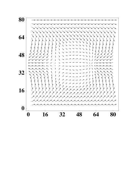
FIG. 1.:

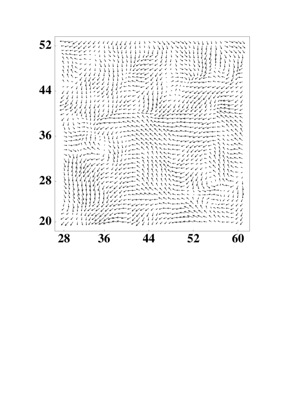
FIG. 2.:

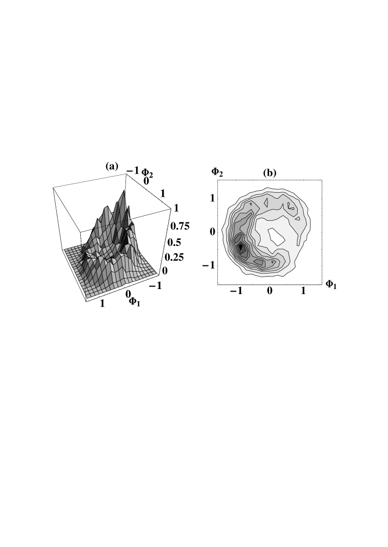
FIG. 3.:

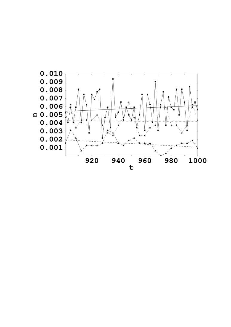
FIG. 4.:

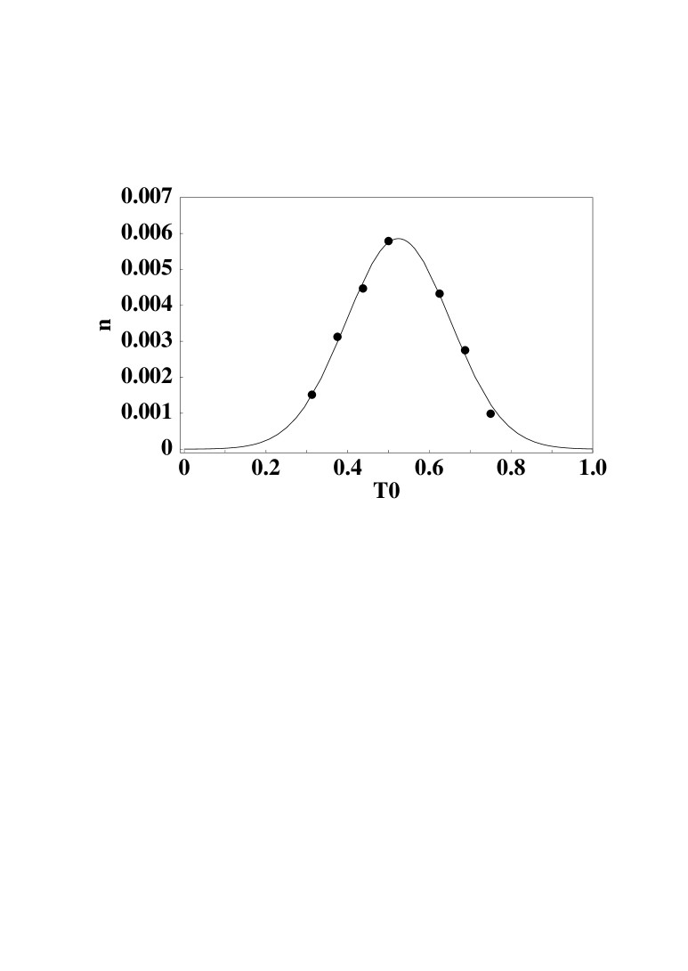
FIG. 5.:

REFERENCES

- [1] A.Vilenkin and E.P.S.Shellard, “Cosmic Strings and Other Topological Defects”, (Cambridge University Press, Cambridge, 1994).
- [2] W.H. Zurek, Phys. Rep. 276, 177 (1996).
- [3] T.W.B. Kibble, J. Phys. A9, 1387 (1976).
- [4] S. Digal, S. Sengupta, and A.M. Srivastava, Phys. Rev. D55, 3824 (1997); ibid Phys. Rev. D56, 2035(1997).
- [5] S. Digal, S. Sengupta, and A.M. Srivastava, Phys. Rev. D58, 103510 (1998).
- [6] J.H. Traschen and R.H. Brandenberger, Phys. Rev. D42, 2491 (1990); Y. Shtanov, J. Traschen, and R. Brandenberger, Phys. Rev. D51, 5438 (1995); L. Kofman, A. Linde, and A.A. Starobinsky, Phys. Rev. D56, 3258 (1997).
- [7] I.I. Tkachev, Phys. Lett. B376, 35 (1996); L. Kofman, A. Linde, and A.A. Starobinsky, Phys. Rev. Lett. 76, 1011 (1996); S. Khlebnikov, L. Kofman, A. Linde, and I. Tkachev, Phys. Rev. Lett. 81, 2012 (1998).
- [8] M.F. Parry and A.T. Sornborger, Phys. Rev. D60, 103504 (1999).
- [9] I.Tkachev, S. Khlebnikov, L. Kofman, and A. Linde, Phys. Lett. B440, 262 (1998).
- [10] S. Kasuya and M. Kawasaki, Phys. Rev. D58, 083516 (1998)
- [11] V. Zanchin, A. Maia, Jr., W. Craig, and R. Brandenberger, Phys. Rev. D60, 023505 (1999).
- [12] L. Gammaitoni, et.al. “Stochastic Resonance”, Rev. Mod. Phys. 70, 223 (1998)
- [13] S. Digal, R. Ray, S. Sengupta, and A.M. Srivastava, hep-ph/9805227.
- [14] A.M. Srivastava, Phys. Rev. D 47, 1324 (1993).
- [15] D. Boyanovsky, H.J. de Vega, R. Holman, and J.F.J. Salgado, Phys. Rev. D54, 7570 (1996).