Nonperturbative corrections to moments of the decay
Christian W. Bauer***bauer@physics.utoronto.ca
Craig N. Burrell†††burrell@physics.utoronto.ca
Department of Physics, University of Toronto
60
St. George Street, Toronto, Ontario,
Canada M5S 1A7
Abstract
We study nonperturbative corrections to the inclusive rare
decay by performing an
operator product expansion (OPE) to .
The values of the matrix elements
entering at this order are unknown and introduce uncertainties into
physical quantities.
We study uncertainties introduced into the partially integrated rate,
moments of the hadronic spectrum, as well as the forward-backward
asymmetry. We find that for large dilepton invariant mass these uncertainties are large. We also assess the
possibility of
extracting the HQET parameters and using
data from this process.
††preprint: UTPT–99-19hep-ph/9911404
I Introduction
Rare decays mediated via flavour changing neutral currents have
received much attention because of their sensitivity to physics
beyond the standard model. In the standard model these decays occur
via penguin and box diagrams with virtual electroweak bosons and up-type
quarks in the loops. Because of the large top quark mass,
the contribution with a top quark in the loop dominates. At energy scales
below the mass of the top quark and boson,
it is convenient to switch to an effective theory where the top quark and
the weak bosons have been integrated out of the theory. The
transition is then mediated by the effective Hamiltonian
[1]
(1)
where the operators are commonly defined by
(2)
(3)
(4)
(5)
(6)
(7)
(8)
(9)
(10)
(11)
Here are the usual
left and right handed chiral projection operators. The values of the
Wilson coefficients have been calculated in
the next to
leading log approximation [2, 3] in the standard
model and are given in
Table I.
-0.240
1.103
0.011
-0.025
0.007
-0.030
-0.311
4.153
-4.546
TABLE I.: The Wilson coefficients in the next-to-leading
log approximation.
Physics beyond the standard model will generally introduce new
contributions to the loop and will therefore
modify the values of these coefficients
[4]. Measurements of the Wilson coefficients may
therefore indirectly constrain new physics scenarios. For example,
the decay is proportional to , and the recent measurements of the
branching ratio [5] and inclusive rate
[6] have placed constraints on models of physics beyond the
standard model which modify the magnitude of [7].
The
decay is suppressed, relative to ,
by an additional factor of
the electromagnetic coupling constant and has not yet been
observed [8]. It has, however, the appeal of
being sensitive to the signs and magnitudes of
, , and , making it a potentially
more powerful probe than of beyond the standard
model physics. Experimental studies of this process impose cuts on the
available phase space.
This is primarily due to the necessity of removing the resonance
from
with the decaying into two leptons. We incorporate
representative cuts into the theoretical analysis.
Using an operator product expansion (OPE) several observables of the
inclusive decay
have been calculated including the leading non-perturbative
corrections [9, 10].
In this framework these leading
corrections arise as matrix elements of dimension five operators, suppressed by
two powers of the quark mass, and are conventionally parameterized
by two quantities, and
. A third parameter
enters through the difference of the quark mass and meson mass
(12)
Whereas can be determined from the
mass splitting, , no such simple relation
exists for . It has been
estimated using various methods to lie in the range [12].
In a previous paper we extended the analysis of the total rate for to
one order higher in the OPE [13].
The dimension six operators arising at this order can be parametrized
by six quantities, commonly labelled
and , all of which are unknown. We found
that the uncertainties introduced
by these six parameters can be significant, depending primarily on the
actual values of the matrix elements and the amount of accessible phase
space. In this paper we give the details of that analysis and also
present calculations for the forward-backward asymmetry and moments
of the hadron invariant mass spectrum at .
As in our
previous analysis, we neglect perturbative
effects and effects due to the finite mass of the quark,
which have been considered elsewhere [10].
It has also been proposed that, rather than use this decay to search for
new physics, it might instead be used to
extract the parameters and through a
measurement of its hadronic invariant mass moments [10].
We estimate the uncertainties in this
extraction due to the unknown matrix elements of the dimension six operators.
This paper is organized as follows. In
section II we briefly introduce the formalism used
to calculate the nonperturbative corrections, and we present the results
for the decay rate in section III. In section
IV we calculate the forward-backward asymmetry of
the lepton pair. We then
proceed in section V to calculate moments of the
hadronic invariant mass spectrum and estimate uncertainties in
extracting and from these moments.
Finally we discuss the results and state our conclusions.
II Operator Product Expansion and Kinematics
The procedure for calculating nonperturbative contributions to
heavy hadron decays has been thoroughly discussed in the
literature [14, 15], and we present here only a brief outline of the
technique. The differential rate is proportional to the product of a
lepton tensor
and a hadron tensor and for the process
in question it may be written as
(13)
where denotes the three body phase space. The spin-summed
tensor for massless leptons is
(14)
The hadron tensor is related via the optical theorem to the
imaginary part of the forward scattering matrix element
where
(15)
In this equation denotes the current mediating this
transition, and is given by
(16)
where is the dilepton
momentum‡‡‡
Notice that this
current reduces to the current when
, , and .
This provides some useful cross-checks with
known results for semileptonic decays [18]..
In accordance with convention, we have defined two effective
Wilson coefficients:
and . The latter contains
the operator mixing of into as well as the one loop
matrix elements of [2, 3].
The full analytic expression for is quite
lengthy and may be found in [3].
Since in the decay of a quark the momentum transfer to the final state parton
is large, the time–ordered product (15)
can be expanded in terms of local operators [14, 15]
(17)
where represents a set of local operators of dimension
, each operator containing derivatives.
For a generic current the expressions for these
operators are quite lengthy. The complete set of operators for
[16] and [17] appear in the literature. In
this study we include operators up to and including dimension .
The standard Lorentz decomposition for the forward scattering amplitude is
(18)
where is the four–velocity of the initial quark .
Since in this paper we treat the final state leptons as massless ,
the form factors do not contribute to observables.
It is clear from (15) and (17) that to
calculate these form factors we must take matrix
elements of the operators . Matrix elements
of dimension four operators
vanish at leading order in the expansion [14] and
matrix elements of dimension five operators may be
parameterized by and [19]
(19)
where , and is an arbitrary Dirac
structure.
Finally, the dimension six operators may
be parameterized by the matrix elements of two local operators
[18, 20]
(20)
(21)
and by matrix elements of two time–ordered products
(22)
(23)
arising from a mismatch between the states of the effective
theory and of the full theory.
The contributions from can most easily be
incorporated by making the replacements [18]
(24)
(25)
in the parton level results.
In addition, as we will show later there is a contribution to the
total rate from the dimension six four–fermion operator
(26)
the matrix element of which we define as
(27)
The form factors up to have appeared in the literature
[9].
The contributions to the form factors proportional to
are presented in Appendix A. The dependence on
is obtained by making
the replacements (25) in the form factors.
The triple differential branching ratio is given by
(28)
(29)
(30)
where we have defined kinematic variables
, ,
and .
In terms of these leptonic variables the limits of phase space are
given by
(31)
(32)
(33)
where .
For the calculation of the hadron invariant mass moments it will be
convenient to express the phase space in terms of
the parton energy fraction and the
parton invariant mass fraction
. They are related to the leptonic variables
introduced above via
(34)
(35)
The phase space can then be expressed as
(36)
(37)
(38)
Since the form factors are independent of , this first
integration is trivial and we arrive
at
(39)
(40)
In the above expressions we use the same conventions as in
[9, 10] and normalize the branching ratio to the semileptonic branching ratio
(41)
introducing the normalization constant
(42)
In this expression is the well-known phase space factor
for the parton decay rate
(43)
and includes the QCD
corrections as well as the nonperturbative corrections up to
(44)
where
(45)
(46)
(47)
(48)
The analytic expression for the perturbative function
can be found in [21].
III The partially integrated branching ratio
An interesting experimentally accessible quantity is the
dilepton invariant mass spectrum.
Evaluating the integral in (28), and doing
the integral over
by picking out the residues, we find for the dilepton invariant mass
spectrum
(55)
The dependence on can be obtained by making the
replacements (25) in (55). In this expression we have
taken the limit . The corresponding expression with full
dependence is given in Appendix B.
FIG. 1.: The differential decay spectrum. The solid line shows the
parton model prediction, the long-dashed line includes the
corrections and the short-dashed line contains all corrections up to .
A plot of this distribution is shown in Fig. 1, where we
have used the values for the nonperturbative matrix elements
(56)
For the matrix elements of the
dimension six operators we use the generic size as suggested by dimensional analysis. The vacuum saturation approximation [22] predicts , as shown, and we find the
displayed spectrum is fairly insensitive to the sign of the other dimension
six matrix elements. One immediately
notices divergences at both endpoints of this
spectrum. The divergence at the endpoint is due to the
intermediate photon going on–shell and is a well known feature of
the decay [1, 9]. In
this limit one expects this spectrum to reduce to the
rate with an on–shell
photon in the final state, convoluted with the fragmentation function giving
the probability for
a photon to fragment into a lepton pair. This correspondence is
explicitly verified by the
analytic form of the divergent term
(57)
where the term multiplying is proportional to the total
rate for
[17]. As mentioned above, experimental cuts require us to stay away
from this endpoint, and therefore automatically regulate this divergence.
The divergence at the endpoint is entirely due to
the operators as can be seen from Fig. 1. In
this case the analytic form of the divergent term is
(58)
This leads, upon integration, to an unphysical
logarithmic divergence in the expression for the total rate that is
regulated by the mass of the quark. (Of course, it is only consistent to
include the mass of the quark in the upper limit of integration if one
uses the spectrum with the full dependence as given in Appendix
B.)
This divergence can be understood by considering a similar effect in the semileptonic
decay [23]. In that context,
the origin of this divergence can be clarified by performing an OPE
for the total, rather than the differential, rate [23, 24].
Including dimension six operators in this OPE one finds a four
fermion operator of the form
(59)
contributing to the rate.
In [23] the matrix element of this operator was calculated at leading order
in perturbation theory by
integrating out the quark and its contribution to the total rate
was found to be .
To calculate this matrix element it was essential
that the mass of the quark be large compared to the QCD scale
. Consequently, for the decay where the same operator with quarks rather than quarks appears, these methods are not
applicable because the quark is too light. Including higher orders in perturbation theory
the matrix element of
the four fermion operator contains logarithms of the form which are
of order unity, making a perturbative calculation of this matrix
element impossible. Thus, a seventh non-perturbative
matrix element defined in (27) is required.
It contributes only at the endpoint of
the spectrum and cancels the logarithmic divergence proportional to
in the total rate
(60)
Another noticeable feature in the dilepton invariant mass spectrum is the
cusp due to the threshold. Near this value of the
methods we used to
calculate the physical spectrum fail because of long distance contributions
from the resonant decay , where the subsequently decays
into two leptons.
Experimentally one deals with this resonance region
by simply cutting it out. Thus, to compare reliably to experiment we
should include such a cut in our calculation. Defining the partially
integrated branching ratio by
(61)
FIG. 2.: The fractional contributions to with respect to
the parton model result from the operators. The
solid, dashed and dotted lines correspond to the contributions from
, and , respectively. The contribution
from is too small to be seen. The two vertical lines
illustrate the positions of the and the resonance.
we plot the contribution of
the individual matrix elements relative to the leading order parton
result in Fig. 2. For the generic size used
in this plot, the contribution from is of the same
size as the contribution from dimension five operators.
This implies that
including the corrections for this decay does not
significantly decrease the
nonperturbative uncertainties. We see that the nonperturbative contributions
become more dominant as the
accessible phase space is decreased§§§We emphasize that the sizes of the
contributions shown here should not be taken as accurate indications
of the actual size of the corrections, but rather as estimates of the
uncertainty in the prediction..
For the
uncertainty from the matrix element is of the same size as
the parton model prediction. This is a clear signal that the OPE is no
longer valid if the phase space is restricted to be too close to the
endpoint . This breakdown of the OPE close to the
endpoint is a well–known feature encountered in this approach to
the study of inclusive decays [26]. Unfortunately, in this endpoint region a
shape function does not exist and an
alternate approach, such as heavy hadron chiral perturbation theory for exclusive final states,
must be used [25].
A cut of has been suggested by the
CLEO collaboration in order to eliminate the resonance region [8].
For this value the partially integrated rate is
(63)
At this value of the cut the coefficients of the nonperturbative matrix
elements clearly indicate a poorly converging OPE. One can estimate the uncertainty
induced by the parameters by fixing to
the values given in (56),
then randomly varying the magnitudes of the parameters
and between and
as suggested by dimensional analysis. We also impose positivity
of as indicated by the vacuum saturation approximation
[22], and we enforce the constraint
(64)
derived from the ground state meson mass splittings
[18]. Here is the
usual coefficient of the beta function for light flavours. Taking the 1
deviation as a reasonable estimate of the uncertainties from
contributions, we find the
uncertainty in to be at the 10% level. It is clear from
(63) that the contribution is large, and
relaxing the positivity constraint on enlarges the
uncertainty to about 20%. A similar statement can be made
regarding the analysis [8] where the phase space cut is slightly higher, and the nonperturbative corrections are correspondingly somewhat larger.
Since the cut on cannot be lowered
because of the resonance, these uncertainties are intrinsic
to our approach in the large dilepton invariant mass region.
It is
important to notice that in the invariant mass region below the
resonance, the uncertainties from these matrix elements are much
smaller.
For example, integrating the differential spectrum up to the cut
specified
in the CLEO analysis [5]
we find
(65)
It is still true that the coefficient of the term
is times larger than that of the term, but both sets of
nonperturbative corrections are small relative to the parton level result in this region.
Although this does not allow us to draw a strong conclusion about the convergence of
the OPE, we can conclude that in this region the nonperturbative corrections
are not a significant source of theoretical uncertainty.
IV The Forward-Backward Asymmetry
The differential forward-backward asymmetry is defined by
(66)
where
(67)
parameterizes the angle between the quark and the
in the dilepton CM frame. It has been shown
[4]
that new physics can modify this spectrum, so it is
interesting to see how terms contribute to the SM
prediction.
Integrating the triple differential decay rate (28) we find
(69)
(71)
Here we have again omitted the trivial dependence on .
It is clear from this expression that the third order
terms do not have
abnormally large coefficients, and therefore introduce only small
variations relative to the second order expression.
An experimentally more useful quantity is the normalized FB asymmetry
defined
by
(72)
Unfortunately, this normalized asymmetry
has inherited the poor behavior of the differential
branching ratio in the endpoint region. In Fig. 3
FIG. 3.: The normalized forward backward asymmetry. The three curves show
the mean value and the uncertainty of the forward
backward asymmetry, obtained in a way similar to that explained in
section
III.
we illustrate
the uncertainties of the normalized FB asymmetry originating from the
matrix elements of the dimension six operators. The three curves show
the mean value and the uncertainty of the forward
backward asymmetry, obtained in a way similar to that explained in
section
III. We can see that up to a value of
the uncertainties are small, but for larger values of the dilepton
invariant mass the uncertainties increase rapidly. Because of the
necessity of the cut to eliminate the resonances, the
accessible high dilepton invariant mass region is therefore restricted
to a few
hundred MeV. For the dilepton invariant mass region below the
resonance the uncertainties are small.
V Extracting and from the hadron
invariant mass moments
Throughout this paper we have fixed the values of the leading
non-perturbative
parameters , , and . However,
these
values must be determined from experiment. The most sensitive
observables
for this purpose are those which vanish in the parton model. It is
interesting to
ask how severely our ignorance of the values of the
parameters compromises our ability to extract the values of
and from such a measurement. It has been suggested by
Ali and Hiller [10] that one use the first
two moments of the hadron invariant mass spectrum defined by
(73)
This idea
is similar to the approaches used in the semileptonic
[18] and the rare radiative decays
[17], though the experimental task is more difficult in this
case due to the small size of the branching ratio.
To calculate these
hadronic moments we relate them to calculable partonic moments
via
(77)
(84)
where we have used the mass relation
(85)
appropriate at this order in the OPE.
We therefore have to calculate the first two moments of the parton
energy and parton invariant mass
, as well as
the mixed moment .
Defining
(86)
we give the results for the required partonic moments in Appendix
C. As before, we have included the dependence on
the cut on the
lepton invariant mass in these results. It is important to note that the
results for the partonic moments given in Appendix C are
expressed in terms of the quark mass and must be
re-expressed in terms of the meson mass using the mass relation
(85). Using again for the cut on the
invariant mass the value proposed by CLEO , we find for the two moments
(88)
(90)
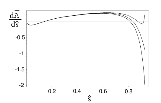
Consider first the expression for . The
term has a small coefficient and tends to cancel against higher order
corrections, making this moment particularly insensitive to .
We can see the problem another way by solving
this equation for : the solution exhibits a pole near
, close to the expected value of [12]. As a result, the extracted value of is extremely sensitive to the values of the higher order parameters.
Since the presence of this pole persists as the value of the cut is
changed, we conclude that this observable is unsuitable for extracting .
For the first moment the convergence of the OPE is much
better. Estimating the uncertainties from the unknown values of the
dimension six operators by the method explained in section
III,
we present the resulting constraint in the plane
in Fig. 4.
FIG. 4.: The constraint in the plane from . The width of the band is entirely
due to uncertainties from operators. The ellipse is the equivalent constraint from moments of semileptonic . It is only the relative orientation, and not location, of the constraints which has meaning.
Superimposed on this figure is the ellipse obtained in
[27] from an analogous study of moments of .
Unfortunately, the bound from our analysis is nearly parallel to the major axis of
this ellipse and, since it is only the relative orientation of the constraints
which has meaning in this figure,
this moment does not provide much additional information about
the values of or .
VI Conclusions
Our purpose in this paper has been to study nonperturbative uncertainties
in the rare inclusive decay . Building on previous
studies which evaluated the leading nonperturbative corrections, we have
parameterized the corrections arising at
in terms of two matrix elements of
local operators , four matrix elements of non local
operators , and one matrix element of a four fermion
operator .
The numerical values of these parameters are unknown, yet even so
a knowledge of the analytic form of the corrections allows us to
study the convergence properties of the operator product expansion in
various regions of phase space. Furthermore, the assumption that
these parameters, being of nonperturbative origin, should be
permits us to make numerical estimates of theoretical uncertainties in
observable quantities.
We first considered the corrections to the differential spectrum
. The experimental spectrum contains two
prominent resonances due to intermediate and production,
and the necessity of cutting these resonances out divides the accessible
spectrum into two parts: the region of low dilepton invariant mass
below the resonance, and the region of high dilepton invariant
mass above the resonance. In the first region, we find that the
parton level calculation dominates, and that nonperturbative corrections
are small. The operator product expansion appears to be converging
according to expectation and, should it be possible to take experimental
data in this region, the results will not suffer from significant
nonperturbative uncertainties.
On the other hand we do find that, as expected, the nonperturbative uncertainties
increase as one moves into the high dilepton invariant mass region. It is
well known that as one approaches this endpoint,
the operator product expansion breaks down. The interesting result of
our study, however, is that the expansion breaks down somewhat earlier than was
anticipated, with the uncertainties coming to
dominate the integrated rate once the available range of is reduced
to about one quarter of the full range. We also showed that the rate
obtained by integrating over the entire region above the resonance
contains uncertainties from dimension six matrix elements at the level,
the uncertainties being dominated by those from the matrix element.
This result may impact the potential for doing precise searches for
new physics using data from this region of phase space.
We also studied the contributions from dimension six operators to the
forward-backward asymmetry. This quantity probes different combinations
of Wilson coefficients than the rate, and has been proposed as a
complimentary source of information about possible new physics effects. As
with the rate, the spectrum is divided into two regions
by the and resonances. We find that the dimension six
contributions are not unduly large anywhere in the phase space, suggesting
that this observable has a well behaved OPE. However
if the differential forward-backward asymmetry is normalized to the
differential rate, the resulting spectrum contains large uncertainties
in the high dilepton invariant mass region. In the region of phase space below
the resonance, however, we find the nonperturbative corrections to
be small.
Finally we addressed a recent proposal suggesting that hadron invariant mass
moments of the differential spectrum for could,
due to the sensitivity of these moments to nonperturbative effects, be used
to constrain the values of the HQET parameters and
. In the low region the moments
are suppressed relative to the rate and, considering the already tiny
branching ratio, it is unlikely that experimental measurements in this region
will be forthcoming. Therefore we focused our attention on the high invariant
mass region. In this region, we found that the first of these
moments provided a constraint in the
plane, but that this
constraint was nearly the same as those derived from other, more
experimentally promising, processes, and therefore seems to be
of limited interest for this purpose. As for the second invariant mass moment
, we found that the nonperturbative uncertainties were such
that it was not possible to extract a stable constraint on the values
of or . From these results, we conclude that
these moments are not well suited to the extraction of these parameters.
VII acknowledgements
We would like to thank Michael Luke for helpful discussions. This work
was supported in part by the National Science and Engineering Research
Council of Canada.
A The contribution of dimension six operators to the form factors
In this appendix we present the form factors .
These form factors have been
calculated previously up to
[9], and we do not reproduce those results
here. We decompose the new contributions arising at as
(A1)
For completeness we have included the full dependence in
these expressions, though in our analysis we set .
Defining with
, and , , we find that the
third order contributions are
(A5)
(A9)
(A12)
(A19)
(A23)
(A28)
(A34)
(A35)
(A38)
B The dilepton invariant mass spectrum with full mass dependence
In this Appendix we present the dilepton invariant mass spectrum for a
finite -quark mass . The spectrum originating from
operators of
dimension has been presented in Eq. (47) of
[9]. The
contributions from the time-ordered operators can be
obtained by making the replacement (25) in this
equation. Since the dilepton
invariant mass distribution is independent of the definition of the
four velocity of the heavy quark, the contribution
proportional to is related by reparameterization invariance
[28] to the contribution. It can be obtained by
the replacement
Thus, the only term we have to add to the existing literature to
obtain the complete expression including all contributions
is the term originating from the Darwin operator whose matrix element
is . This contribution is given by
The function is singular at the upper limit of integration.
To regulate this divergence we defined a “star function”
(B5)
This “star function” is analogous to the common plus distribution.
The functions appearing above are
(B9)
(B14)
(B18)
(B19)
Notice that these terms correctly reproduce the expression (55)
in the limit .
C The moments up to with a cut on the
dilepton invariant mass
We write the moments in the form
(C1)
where is given in Eq. (61).
The coefficient depends on the parameters
and as explained in section II, so we express
the moments and as integrals which
we evaluate numerically,
(C2)
(C3)
(C5)
For the other contributions we find
(C9)
(C14)
(C18)
(C23)
(C27)
(C31)
(C34)
(C37)
(C41)
(C45)
REFERENCES
[1]B.Grinstein, M.Savage, and M.B.Wise, Nucl. Phys. B319 (1989) 271.
[3] A.J. Buras and M.Münz, Phys. Rev. D 52 (1995) 186.
[4] A.Ali, G.F.Giudice, and T.Mannel, Z.Phys.C67 (1995) 417; C.Huang, W.Liao, and Q.Yan, Phys. Rev. D 59 (1999) 011701; P.Cho, M.Misiak, and D.Wyler, Phys. Rev. D 54 (1996) 3329; J.Hewett and J.D.Wells, Phys. Rev. D 55 (1997) 5549; T.Goto, Y.Okada, Y.Shimizu, and M.Tanaka, Phys. Rev. D 55 (1997) 4273; E.Lunghi, A.Masiero, I.Scimemi, and L.Silvestrini, hep-ph/9906286.
[5]R. Ammar et al. (CLEO Collaboration),Phys. Rev. Lett. 71 (1993) 674.
[6]M.S. Alam et al. (CLEO Collaboration), Phys. Rev. Lett. 74 (1995) 2885; hep-ph/9908022.
[7] J.Hewett, hep-ph/9406302; T.G.Rizzo, Phys. Rev. D 58 (1998) 114014; F.Borzumati and C.Greub, Phys. Rev. D 58 (1998) 074004; W.de Boer et al., Phys. Lett. B 438 (1998) 281; H.Baer et al., Phys. Rev. D 58 (1998) 015007; M.Ciuchini et al., Nucl. Phys. B527 (1998) 21; J.Agrawal et al., Int. Jour. Mod. Phys. A11 (() 1996) 2263; M.A.Diaz et al., Nucl. Phys. B551 (1999) 78; G.V.Kranrotis, Z.Phys.C71 (1996) 163; A.L.Kagan and M.Neubert, Eur.Phys.J.C7 (1999) 5.
[8] S. Glenn et al. (CLEO Collaboration), Phys. Rev. Lett. 80 (1998) 2289; B.Abbott et al. (DØ Collaboration), Phys. Lett. B 423 (1998) 419; C.Albajar et al. (UA1 Collaboration), Phys. Lett. B 262 (1991) 163. Also, a recent search in exclusive channels: T.Affolder et al. (CDF Collaboration), hep-ex/9905004.
[10] A. Ali and G. Hiller, Phys. Rev. D 58 (1998) 074001.
[11]B.Grinstein, M.Savage, and M.B.Wise, Nucl. Phys. B319 (1989) 271.
[12] Z.Ligeti, Y.Nir, Phys. Rev. D 49 (1994) 4331; M.Gremm,
A.Kapustin, Z.Ligeti, M.Wise, Phys. Rev. Lett. 77 (1996) 20; M.Neubert,
Phys. Lett. B 389 (1996) 727.
[13] C. Bauer and C.Burrell, Phys. Lett. B 469 (1999) 248.
[14]J. Chay, H. Georgi and B. Grinstein, Phys. Lett. B247 (1990) 399.
[15]I.I. Bigi, M. Shifman, N.G. Uraltsev,
A. Vainshtein, Phys. Rev. Lett. 71
(1993) 496, B. Blok, L. Koyrakh, M. Shifman, A. Vainshtein,
Phys. Rev. D49 (1994) 3356, Erratum-ibid. D50 (1994) 3572,
A. V. Manohar, M. B. Wise, Phys. Rev. D49 (1994) 1310; I.I.Bigi, N.G.Uraltsev, A.I.Vainshtein, Phys. Lett. B 293 (1992) 430; Erratum, Phys. Lett. B 297 (1993) 477.
[16] A.Falk, M.Luke, and M.Savage, Phys. Rev. D 49 (1994) 3367.
[18]M. Gremm and A. Kapustin, Phys. Rev. D55 (1997) 6924.
[19]A.F. Falk and M.Neubert, Phys. Rev. D47 (1993) 2965;
Phys. Rev. D 47 (1993) 2982.
[20]T. Mannel, Phys. Rev. D50 (1994) 428.
[21]A. F. Falk, M. Luke, M. Savage, Phys. Rev. D53 (1996) 2491.
[22]
M.A. Shifman and M.B. Voloshin, Sov. J. Nucl. Phys. 45 (1987) 292;
M.B. Voloshin, N.G. Uraltsev, V.A. Khoze and M.A. Shifman,
Sov. J. Nucl. Phys. 46 (1987) 112.
[23]B. Blok, R.D. Dikeman and M. Shifman, Phys. Rev. D51,
6167 (1995).
[24]C. Bauer, A. Falk and M. Luke, Phys. Rev. D 54 (1996) 2097.
[25] G.Buchalla and G.Isidori, Nucl. Phys. B525 (1998) 333.